Generalized Label-Efficient 3D Scene Parsing via Hierarchical Feature Aligned Pre-Training and Region-Aware Fine-tuning

Abstract

Deep neural network models have achieved remarkable progress in 3D scene understanding while trained in the closed-set setting and with full labels. However, the major bottleneck for the current 3D recognition approach is that these models do not have the capacity to recognize any unseen novel classes beyond the training categories in diverse kinds of real-world applications. In the meantime, current state-of-the-art 3D scene understanding approaches primarily require a large number of high-quality labels to train neural networks, which merely perform well in a fully supervised manner. Therefore, we are in urgent need of a framework that can simultaneously be applicable to both 3D point cloud segmentation and detection, particularly in the circumstances where the labels are rather scarce. This work presents a generalized and simple framework for dealing with 3D scene understanding when the labeled scenes are quite limited. To extract knowledge for novel categories from the pre-trained vision-language models, we propose a hierarchical feature-aligned pre-training and knowledge distillation strategy to extract and distill meaningful information from large-scale vision-language models, which helps benefit the open-vocabulary scene understanding tasks. To leverage the boundary information, we propose a novel energy-based loss with boundary awareness benefiting from the region-level boundary predictions. To encourage latent instance discrimination and to guarantee efficiency, we propose the unsupervised region-level semantic contrastive learning scheme for point clouds, using confident predictions of the neural network to discriminate the intermediate feature embeddings at multiple stages. In the limited reconstruction case, our proposed approach, termed WS3D++, ranks 1st on the large-scale ScanNet benchmark on both the task of semantic segmentation and instance segmentation. Also, our proposed WS3D++ achieves state-of-the-art data-efficient learning performance on the other large-scale real-scene indoor and outdoor datasets S3DIS and SemanticKITTI. Extensive experiments with both indoor and outdoor scenes demonstrated the effectiveness of our approach in both data-efficient learning and open-world few-shot learning. All codes, models, and data are to made publicly available at: https://github.com/KangchengLiu. The code is at: WS3D++ Code link.

1 Introduction

The 3D scene parsing problem, which typically encompasses several important downstream tasks: point cloud semantic segmentation, instance segmentation, and object detection, becomes increasingly important with the wide deployment of 3D sensors, such as LiDAR and RGB-D cameras [1, 2, 3, 4, 5, 6, 7, 8]. Point clouds are raw sensor data obtained from 3D sensors and the most simple and common 3D data representation for understanding 3D scenes of robot navigation, robot grasping, and manipulation tasks. Despite significant success in deep neural networks applied to 3D visual perception, two major challenges hinder the construction of more scalable visual perception systems in 3D worlds. One is the closed-set assumption, which means the model only performs well while recognizing the categories that appear in the training set and struggles in recognizing the novel unseen object categories or concepts. Another is the heavy reliance on large amounts of high-quality labeled data. Large-scale 3D scenes are very laborious to label, which also makes it very hard for deep network models to perform well with very limited annotations.

Close-set assumption: One of the major bottlenecks in scaling up visual perception systems is the poor generalization capacity while encountered with diverse novel semantic classes or severe domain shifts. To endow the model with the capacity for adapting the learned representation and make it conform to different data distributions as well as recognize diverse novel categories, pioneer researches such as CLIP [9], Flamingo [10], and Otter [11] have demonstrated the great potentials in learning well-aligned visual linguistic representation from large-scale image-text pairs on the Internet for improving the model generalization capacity. To this end, subsequent approaches have been proposed in establishing abundant vision-language associations for different visual recognition tasks including detection and segmentation using the large-scale vision-language model (VLM) [12, 13, 14]. The paired visual-linguistic feature representation can enable the recognition of a large number of novel objects or concepts with natural language supervision because the visual and the lexical language features are well-matched in their shared semantic feature space. Despite the remarkable performance achieved in developing diverse vision-language foundation models such as SAM [15] and SEEM [16] for image-based scene understanding, it remains very difficult for CLIP [9] to benefit downstream 3D scene understanding because it is difficult to raise the feature dimension to 3D and establish explicit correlations or find clear alignments between large-scale scene/object-level 3D point clouds as well as linguistic semantic concepts. Moreover, it is even harder to transfer the informative knowledge to various downstream 3D scene understanding tasks. These limitations severely restrict the scalability of VLM to handle diverse unseen 3D scenes containing diverse novel 3D object categories.

Reliance on large-scale labeled data. A critical prerequisite for fully exploiting the capacity of the fully supervised deep learning approaches is the accessibility to large-scale well-annotated high-quality training data. Most point cloud understanding methods rely on heavy annotations [17, 18, 19]. However, the annotation of large-scale 3D point cloud scenes is rather time-consuming and labor-intensive. For instance, it requires around thirty minutes to label a single scene for ScanNet [20] or S3DIS [21] with thousands of scenes. Though existing point cloud understanding methods [17, 18, 19] have achieved decent results on these datasets, it is difficult to directly extend them to novel scenes when the high-quality labeled data is scarce. In the meanwhile, it is often the case that a limited number of scenes can be reconstructed in real applications [22]. Therefore, developing methods that can be trained with very limited labeled scenes, termed data-efficient 3D scene understanding with limited scene-level annotation, becomes in high demand. Data-efficient semantic and instance segmentation [23, 24, 25] is a vehement research topic for image-level scene understanding. Some simple but successful methods have been proposed, such as contrastive learning [26, 27] which learns a meaningful and discriminative representation, and conditional random field (CRF) [28, 29] for pseudo label propagation. However, there still exist four main challenging unsolved issues while scaling up these approaches to 3D scene understanding. First, the widely adopted energy function-based conditional random field segmentation [29] relies on handcrafted feature similarities and does not consider explicit boundary information. It attaches equal importance to pixels on semantic boundaries and within same semantic objects, which can cause vague and inaccurate predictions in pixel-level segmentation at object boundaries. And how to leverage boundary information has been explored in 2D but rarely explored in 3D data efficient learning [30]. Second, the computation costs are both very high when applying point-level contrastive learning or point-level energy-based segmentation in a dense point cloud scene for every point pair [31]. Furthermore, large-scale point cloud scenes even contain billions of points, making point-level contrastive learning intractable in computational costs. Third, the existing unsupervised contrastive learning-based pre-training for point clouds [27, 22, 32, 33] only considers geometrically registered point/voxel pairs as the positive samples, while it does not explicitly consider explicit regional information, let alone the hierarchical alignments.

Figure 1: Overall illustrative diagram of our proposed WS3D++. We integrate language-3D feature associated pre-training and data-efficient fine-tuning to achieve effective data-efficient and open-vocabulary 3D scene understanding for 3D scenes.

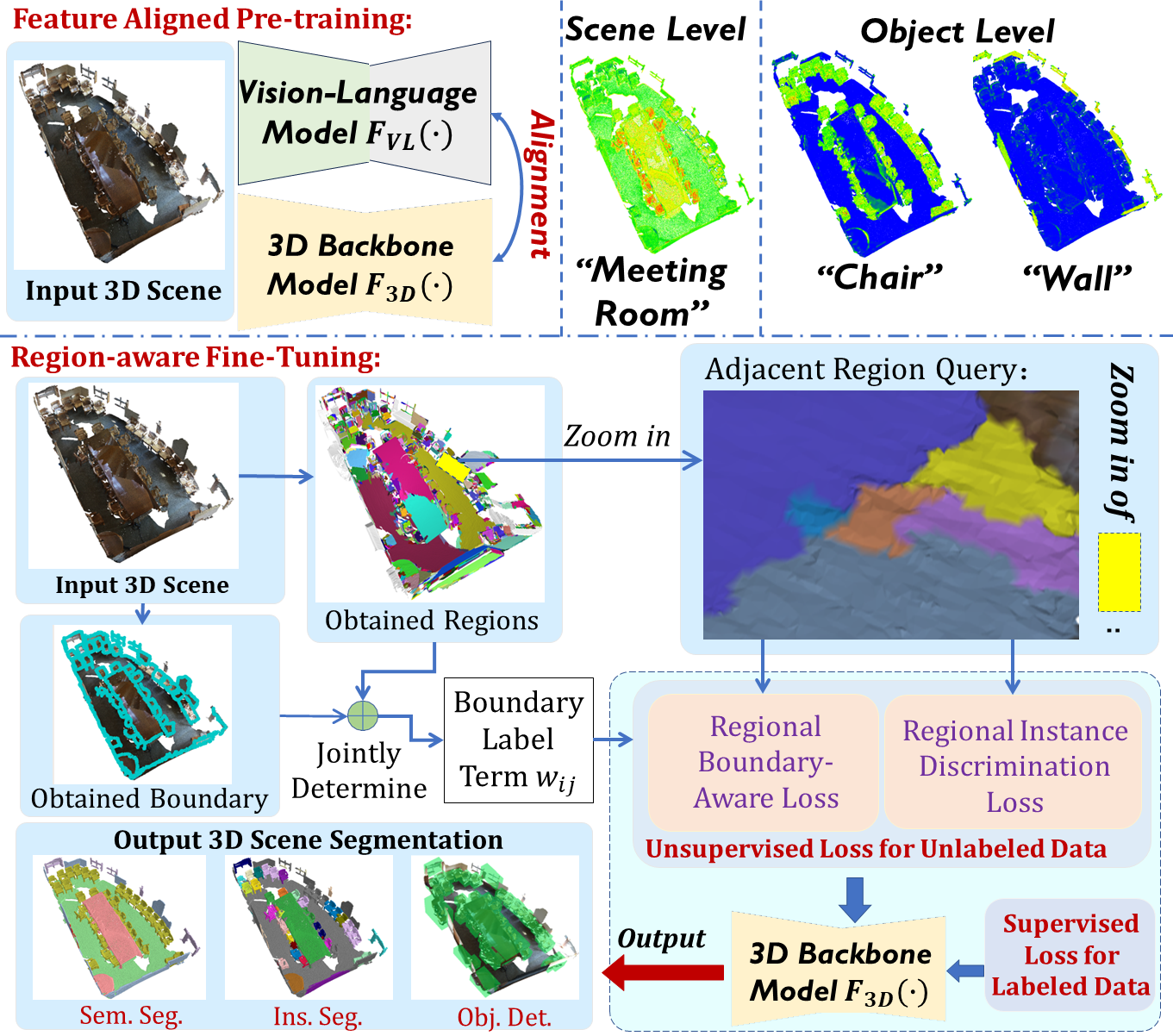
Driven by the above motivations in terms of both generalization capacity and data efficiency, we propose an effective two-stage framework, involving unsupervised hierarchical vision-language pre-training and label-efficient fine-tuning to enable more label/data-efficient 3D scene understanding. As shown in Fig. 1, in the pre-training stage, we leverage the rendering techniques to construct well-aligned 2D views for large-scale 3D scenes to establish more accurate coarse-to-fine vision-language associations. Then, we leverage the off-the-shelf object detector and the pre-trained large-scale vision-language model CLIP [9] to construct the hierarchical feature representations from both the global scene level to the local object level. We also propose an effective knowledge distillation strategy that distills the informative visual-language-aligned representation of the image encoder in CLIP [9] to the 3D backbone network.

During the fine-tuning stage, as shown in Fig. 1, we propose a unified WS3D++ framework that simultaneously solves the 3D scene understanding problem under the data-efficient setting. We first use the over-segmentation [34] to obtain regions and use a boundary prediction network (BPN) as an intermediate tool to obtain boundary region labels. Then, high-confidence boundary region labels serve as the guidance for our proposed region-level energy-based loss. Meanwhile, we propose a region-level confidence-guided contrastive loss to enhance instance discrimination. Specifically, our WS3D++ includes two innovative designs to address the very challenging label scarcity issues and to enhance performance. Firstly, to encourage latent instance discrimination and to guarantee efficiency, an efficient region-level feature contrastive learning strategy is proposed to guide network training at multiple stages, which realizes the unsupervised instance discrimination. Also, to leverage boundary information as labels for the final semantic divisions, an energy-based loss with guidance from the semantic boundary regions is proposed to take the maximized advantage of the unlabeled data in network training. Combined with supervised loss, the labeled data can also be leveraged to boost the final downstream 3D scene understanding performance.

WS3D++ is a significant extension of the preliminary version of the conference work WS3D [4], where basic ideas of boundary awareness and contrastive instance discrimination are introduced to tackle the data-efficient 3D scene understanding during fine-tuning stage. In summary, we extensively enriched previous works in the following aspects:

First, we propose a generalized pre-training approach for data-efficient learning, which establishes accurate alignments between language and 3D point cloud in terms of both object-level and scene-level semantics in a hierarchical manner.  Second, we propose to leverage rendering techniques which make explicit associations between image and point cloud to facilitate 2D-to-3D matching and subsequent language-to-3D matching.  Third, we visualized the language-queried activation maps directly on the 3D scenes, which demonstrates that the proposed approach learns better visual-linguistic alignment between the language descriptions and the visual object-level information. Finally, we evaluate our proposed approach comprehensively in diverse data-efficient and open-world learning settings for both the 3D semantic segmentation and 3D instance segmentation tasks.

The contributions of our work are highlighted as follows:

1. During the pre-training stage, we first design an effective approach which distills rich knowledge from the large-scale vision-language model into the 3D point cloud modality. Specifically, we propose leveraging rendering to obtain explicit scene-level and object-level 2D-3D feature associations, establishing a more accurate vision-language association hierarchically than the original CLIP encoder.

2. During the pre-training stage, we further propose a word-to-3D matching approach to establish the well-aligned language-3D associated feature representations at both the scene level and the object level, which largely facilitates the subsequent effective contrastive learning with the mostly matched visual-linguistic contrastive pairs. The proposed designs have both enhanced the data-efficient learning and the knowledge-transfer capacity of the model, as demonstrated by our extensive experiments on both the 3D object detection and the 3D semantic/instance segmentation tasks.

3. During the fine-tuning stage, we propose a region-aware energy-based optimization approach to achieve the region-level boundary awareness, which utilizes the boundary as additional information to help assist the 3D scene segmentation and understanding. Furthermore, we propose the unsupervised region-level semantic contrastive learning strategy for multi-stage feature discriminations. The energy-based loss and the contrastive loss are jointly optimized for pre-training the backbone network in a complementary manner, which take full advantage of the unlabeled data.

4. Integrating the above two stages as a whole, we propose a unified framework termed WS3D++. State-of-the-art performance has been achieved by it with extensive experiments conducted on ScanNet [20] and other indoor/outdoor benchmarks such as S3DIS [21], SemanticKITTI [18] and NuScenes [35] in diverse experimental settings without bells and whistles. Finally, our proposed approach achieves pioneer performance on the very large-scale ScanNet [20] dataset in diverse downstream tasks of 3D scene understanding, including tasks among 3D semantic segmentation, 3D instance segmentation, and 3D object detection.

To the best of our knowledge, this is the pioneer work which comprehensively evaluates across diverse 3D label-efficient scene understanding downstream tasks with our proposed 3D open-vocabulary recognition approach termed WS3D++. Our endeavor is orthogonal to the 3D backbone network designs and thus can be seamlessly integrated with the prevailing 3D point cloud detection or segmentation models. Our comprehensive results provide solid baselines for future research in data-efficient 3D scene understanding.

2 Related Work

Learning-based Point Cloud Understanding. Deep-network-based approaches are widely adopted for point cloud understanding. Fully supervised approaches can be roughly categorized into voxel-based [36, 37, 38, 39, 40], projection-based [41, 42, 43, 44, 45, 46], and point-based approaches [47, 48, 49, 50, 51, 52, 53, 54, 55, 56, 57, 58]. The voxel-based approaches [59, 60, 61] which are built upon SparseConv [59] and voxelize the point cloud for efficient processing have achieved remarkable performance in 3D scene parsing. Therefore, we use SparseConv [59] as our backbone architecture for downstream semantic understanding tasks because of its high performance in inferring 3D semantics. Also, the LiDAR-based approaches are of significance to many industrial applications such as inspections [62, 63, 64] and robot localization [65, 66, 67, 68, 69], and large-scale robotic scene parsing [57, 70, 71], as well as robotic control applications [72, 73, 74, 75, 76, 77], etc.

Pre-training for 3D Representation Learning. Many recent works propose to pre-train networks on source datasets with auxiliary tasks such as low-level point cloud geometric registration [27], 3D local structural prediction [78], the completion of the occluded point clouds [79], and the foreground-background feature discrimination [58], with effective learning strategies such as contrastive learning [27] and masked generative modelling [80, 81]. Then they finetune the weights of the trained networks for the downstream target tasks to boost their performances. However, several major challenges still exist. First, the above pre-training approaches all rely on the closed-set assumption, which means that the model can barely be transferred to recognize novel categories that do not appear within the training data. Second, the above methods require accessibility to the well-registered augmented point cloud [27, 22, 32, 33] to construct the pre-training contrast views, which are very hard to obtain for large-scale 3D scenes. Third, a large number of computational power is required in the pre-training stage. Therefore, the designed pre-training approaches need to be very simple and lightweight, thus will make it easier to directly transfer the model to large-scale point clouds.

Recently, with the development of large-scale vision-language models such as CLIP [9] and Flamingo [10], we can largely benefit the recognition capacity of 3D scene understanding models by distilling knowledge from large-scale vision-language models. For example, some pioneer works such as PointCLIP [82, 83] and ULIP [84] successfully transfer the knowledge from vision-language models to boost the downstream 3D shape classification tasks. The 3D CAD shapes are transferred to multi-view depth maps, thus they can be fed into the CLIP visual encoder and used the image representations paired with the corresponding point cloud as a bridge to obtain the correlations between the 3D and textual features. Moving beyond object-level recognition tasks, pioneer works also explore how to establish alignment among images, language, and 3D point cloud scenes for the task of open-vocabulary 3D scene understanding [85, 86, 87], which target localizing, detecting, and segmenting novel object categories that do not exist in the annotation. Compared with them, our proposed simple but effective framework can be both applicable to data-efficient learning and open-vocabulary scene understanding.

Figure 2: The pre-training paradigm of our proposed WS3D++. We propose hierarchical feature alignments to establish hierarchical vision-language aligned feature representations during pre-training. This kind of paradigm helps learn more powerful visual-linguistic matched representations ranging from both the global view-level to the local object category-level.

Label/Data-Efficient Learning for 3D. Recent studies have produced many elaborately designed backbone networks for 3D semantic/instance segmentation [88, 89, 45, 90, 91], as well as for 3D object detection [92, 93, 94, 95]. However, they rely on full supervision. Directly applying current SOTAs (State-of-the-art) methods for training will result in a great decrease in performance [96] for WSL, if the percentage of labeled data drops to a certain value, e.g., less than 30%. Recently, many works have started to focus on point cloud semantic segmentation with partially labeled data. Wang et al. [97] choose to transform point clouds to images, but pixel-level semantic segmentation labels are required for network training. Sub-cloud annotations [98] require extra labor to separate the sub-clouds and to label points within the sub-clouds. Liu [99] proposed a robust data-efficient 3D scene parsing framework. It leverages the complementary merits of the superior generalization capacity of the traditional 3D descriptors and the strong feature description capacity learned 3D descriptors to learn very robust local features. Then using the descriptor guided learned region merging [3], superior performance can be achieved on downstream tasks. Liu et al. [100, 101] proposed self-training techniques to tackle scene understanding in weak supervision, which design a two-stage training scheme to produce iteratively optimized pseudo labels from weak labels during training. Despite satisfactory results, these approaches still have not learned generalized representation applicable to diverse tasks. Xu et al. [102] adopt a weakly-supervised training strategy, which combines training with coarse-grained information and partial points using 10% labels. However, their tested cases are limited to object part segmentation, and it is difficult to uniformly choose points to label. The convex decomposition [103] is conducted in an approximate manner to perform 3D scene parsing on the object parts. More approaches [104] have been proposed recently, which utilize class prototypes and masked point cloud modeling [105, 106, 81] to learn informative representations for downstream 3D scene understanding. To sum up, although approaches have been proposed to alleviate the data efficiency problem, the models for weakly supervised learning lack the capacity to recognize novel categories beyond the labeled training set. Our framework tackles both open-set and data-efficient learning problems and is widely applicable to diverse 3D scene understanding downstream tasks.

3 Proposed Methodology

We propose a general WS3D++ framework to tackle weakly supervised 3D understanding with limited labels, as demonstrated in Fig. 1. Our framework consists of both the vision-language pre-training stage shown in Fig. 2 and fine-tuning stage illustrated in Fig. 3. During the pre-training stage, we first propose the hierarchical contrastive learning strategy with the help from rendering for more accurate vision-language alignments at both the scene level and object level. Then we also design a distillation strategy to distill point-language-aligned representations from 2D image network to 3D point-cloud network to endow 3D networks with the open-vocabulary recognition capacity. Finally, during the fine-tuning stage, we directly propose a weakly supervised approach, we perform fine-tuning with regional boundary awareness and region-aware instance discrimination, which significantly improve model discrimination capacities when the labeled data are rather scarce.

Figure 3: The fine-tuning paradigm of our proposed WS3D++, i.e. WS3D. WS3D [4] consists of three modules: 1. The unsupervised region-level energy-based optimization guided by boundary labels; 2. The unsupervised multi-stage region-level contrastive learning with high confidence; 3. The supervised region-level semantic contrastive learning with labeled data. The backbone network adopts encoder-decoder structures. The weights of the backbone network are shared in the supervised and unsupervised branches. Integrated with the proposed pre-training paradigm illustrated in Figure 2, by our proposed hierarchical feature aligned pre-training and regional fine-tuning, more effective label-efficient learning as well as open-vocabulary learning is realized.

3.1 Hierarchical Vision-Language Knowledge Associations and Distillations for Pre-training

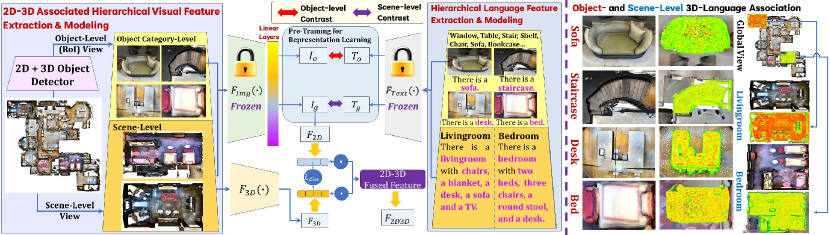
We propose a hierarchical alignment strategy in pre-training, which employs the rendering approach as a bridge to effectively align 3D vision and language embeddings, thus capturing coarse-to-fine associations for visual-linguistic synergized representations from the global scene level to local object level. It enables extracting more accurate 3D-language associations in a hierarchical manner.

Multi-view rendering. To obtain paired 2D-3D representations, we propose leveraging multi-view rendering to obtain paired 2D views from 3D point cloud scenes. The pairing process consists of two steps, the first is to convert point cloud scenes into meshes and the second is to render 2D images based on the different views of the 3D meshes. In terms of point-to-mesh transformation, we utilize the Delaunay triangulation approach [107, 108] to convert the point cloud into meshes, which is demonstrated as a very effective method for surface reconstruction. It connects the points in point cloud scenes by forming triangles that satisfy the Delaunay criterion which guarantees no point lies inside the circumcircle of any triangle. This method generates a triangle mesh that approximates the surface of the point cloud [109]. In terms of mesh-to-image transformation, we leverage the rendering pipeline including the vertex transformation, projection, and rasterization, as well as shading. We directly use the rendering library OpenGL [110] to render images from the meshes. The process involves projecting the 3D vertices onto a 2D image plane based on camera parameters and applying shading and lighting calculations of 3D meshes to determine the specific color of each pixel. By this simple design, the world-to-camera extrinsic matrix $T_{e}$ containing both rotation and translation information between the 2D pixels and 3D points can be easily obtained.

2D to 3D Alignment. After multi-view rendering, the strict 2D-3D alignment can be easily established if the camera’s intrinsic $T_{i}$ is obtained from the standard calibration [111] and the extrinsic $T_{e}$ is obtained from the rendering. To be more specific, given the 3D point $\textbf{p}_{3D}\in\mathbb{R}^{3}$ as well as its 2D corresponding pixel coordinate $\textbf{p}_{2D}=(u,v)$, if we consider the pin-hole camera model, the transformation can be represented as $\hat{\textbf{p}}_{2D}=T_{i}~{}\cdot~{}T_{e}~{}\cdot\hat{\textbf{p}}_{3D}$. The $\hat{\textbf{p}}_{2D}$ and $\hat{\textbf{p}}_{3D}$ are represented within the homogeneous coordinates, and they are strictly paired. Therefore, we can strictly determine the correspondence between $\hat{\textbf{p}}_{2D}$ and $\hat{\textbf{p}}_{3D}$. Moreover, we can find an explicit association between each element of the textual feature $\textbf{F}_{T}$ and the 3D feature $\textbf{F}_{3D}$ while passing through the backbone network.

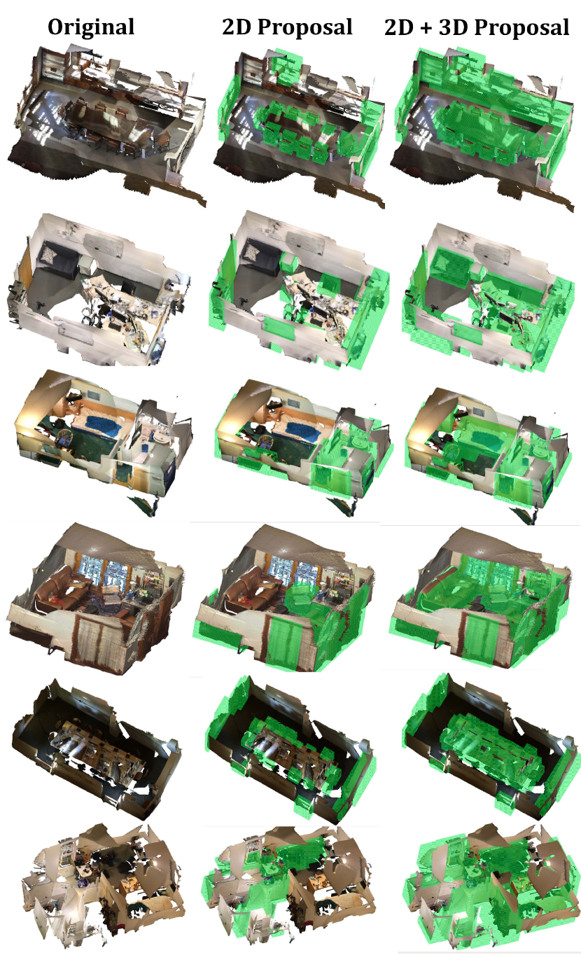
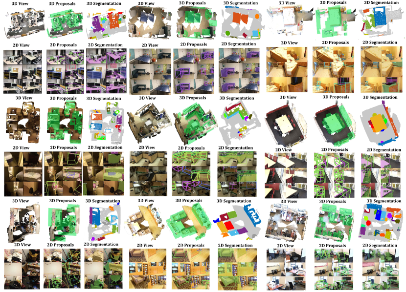
United 2D and 3D Proposal Generation. As shown in Fig. 6, according to our experiments, we found that it is difficult to directly find the object-level information merely based on the 2D proposals due to the great information loss while conducting rendering, the proposals provided by the 2D region proposal network (RPN) [112] can not effectively capture the 3D object information within the scene. On the other hand, merely relying on the 3D proposal provided by the 3D RPN [113] still can not guarantee accurate proposal generation for the fact that some objects are too adjacent in their geometry. To this end, we propose to leverage the union of 2D and 3D RPN to capture intact and all-inclusive proposals within the 3D scenes. Denote the region proposals as $R_{2D}$ and $R_{3D}$ respectively, the final holistic proposal generation $R_{H}$ is formulated as $R_{H}=R_{2D}\cup R_{3D}$. According to our experiments, this simple design can considerably boost the performance for the fact that the objects are more clustered and closely distributed within the indoor scenes. Taking the union of 2D and 3D object proposals into consideration also guarantees that the optimization merely considers the regions where the object really exists and prevents the models from taking the pure background into consideration during the optimizations.
Scene-level Sentence-3D Matching. We perform image-language alignment at both the object level and the scene level to pre-train the backbone network, which captures very accurate language-2D association for rendered images. The alignment at the object level allows the capturing of the fine-grained object-to-semantic concept matching, while the alignment at the scene level captures both holistic scene-level information and the dependent relations between the objects and holistic 3D scenes. For example, the bed exists in the bedroom while the sofa and TV lie in the living room with a clear owner-member relationship. To capture the object proposal information from the rendered images, we utilize the region proposal network (RPN) [112] to obtain the class-agnostic regions. For the text descriptor within the region, we use three most similar noun phase extract by it given by CLIP [9], which captures the scene level and the object level image patches with the most relevant texture description. Then we pass through both the original scene-level image as well as the obtained region-level image into the frozen CLIP visual encoder to obtain the scene-level visual feature $\textbf{I}_{\textbf{g}}$ as well as the object-level visual feature $\textbf{I}_{\textbf{l}}$, respectively. As shown in Figure 2, in order not to influence the well-learned feature representations provided by the CLIP encoder, we freeze the backbone and merely add a linear projection layer at the end of the network to facilitate the adaptive hierarchical feature-aligned pre-training.

Global and Regional Word-3D Matching. At the next step, we perform regional word-to-3D matching. We use the CLIP image encoder to generate a set of local feature embeddings $\textbf{F}^{l}_{3D}$ for the rendered proposal-level image patches, and the set of global embedding $\textbf{F}^{g}_{3D}$ for the whole scene. While the text encoder extracts the local textual embeddings $\textbf{F}^{l}_{T}\in\mathbb{R}^{H\times D}$ and the global textual embeddings $\textbf{F}^{g}_{T}$. The operation can be interpreted as a bi-directional operation, which means that for each region proposal image patch, we find the textual concept that matches best with the semantics of the region. And for each textual concept, we find the multiple regions that correspond with it. Next, we calculate the cosine similarity $\mathcal{G}_{sim}$ between the 3D visually encoded features and the textual features:

$$\textbf{S}(\textbf{I},\textbf{T})=\mathcal{G}_{sim}(\textbf{F}^{l}_{3D},\textbf{F}^{l}_{T})+\mathcal{G}_{sim}(\textbf{F}^{g}_{3D},\textbf{F}^{g}_{T})$$ (1)

We model it as an optimal transport problem, which finds the most similar visual feature by formulating it as the differentiable Top-$k$ with respect to the anchor textual description [114] both globally and regionally. The region-to-word pairs with Top-$k$ maximum activations $\textbf{S}(\textbf{I},\textbf{T})$ are finally regarded as the positive pairs in contrast, ensuring learning highly discriminative representations.

Contrastive Optimizations. Note that when conducting contrastive learning, we regard textual features as anchors because textual descriptions are highly semantic and contain rich information, whereas the images contain too much low-level information and pixel-level details. Denote the $\textit{{F}}^{\;b,+}_{3D}$ and the $\textit{{F}}^{\;b,-}_{3D}$ as the positive and the negative features with respect to the anchor textual feature $\bm{F}_{T}^{a}$, respectively, the designed contrastive loss is formulated as follows:

$$\bm{\mathcal{L}}_{Ctr}=-\frac{1}{\|\textbf{H}\|}\sum_{(a,b)\in\textbf{H}}\log\frac{\exp(\bm{F}_{T}^{a}\cdot\textit{{F}}^{\;b,+}_{3D}/\tau)}{\sum_{(\cdot,c)\in\textbf{B}}\exp(\bm{F}_{T}^{a}\cdot\textit{{F}}^{\;b,-}_{3D}/\tau))}.$$ (2)

$$\mathcal{L}^{total}_{Ctr}=\mathcal{L}^{G}_{Ctr}+\mathcal{L}^{L}_{Ctr}$$ (3)

3D Language Distillation. We utilize the $\mathcal{KL}$ divergence as the distillation loss to further distill the knowledge from 2D feature space to 3D. Compared with the mean square error loss such as the $\mathcal{L}_{1}$ or $\mathcal{L}_{2}$ losses, the $\mathcal{KL}$ divergence has improved regression capacity and ensured smoother gradient [115], which to some extent overcomes overfitting problems while distilling knowledge. The distillation loss $\mathcal{L}^{Dist}_{\mathcal{KL}}$ is formulated as:

$$\vspace{-0.02mm}\mathcal{L}^{Dist}_{\mathcal{KL}}=\textbf{Div}_{\mathcal{\small{KL}}}(\textbf{F}_{2D}\|\textbf{F}_{3D})\vspace{-0.02mm}$$ (4)

The pre-training optimization loss is the joint considerations of hierarchically matched contrastive optimization and 3D-Language distillation with balancing $\lambda_{\mathcal{\small{KL}}}$ set to 0.5 empirically:

$$\mathcal{L}_{Pretrain}=\mathcal{L}^{total}_{Ctr}+\lambda_{\mathcal{\small{KL}}}\mathcal{L}^{Dist}_{\mathcal{KL}}$$ (5)

According to our extensive experiments, our simple pre-training approach provides well-aligned vision-language-3D co-embedding. It largely facilitates vision-language-associated knowledge transfers from 2D to 3D, boosting both the label efficiency and the final recognition capacity of novel categories.

3.2 Region-Aware Fine-tuning

During the fine-tuning stage, our proposed framework consists of three subparts for the network optimization: 1. Unsupervised energy-based loss guided by boundary awareness and highly confident network predictions for unlabeled data, which is discussed in 3.2.1; 2. Unsupervised multi-stage region-level contrastive learning with highly confident predictions for unlabeled data, which is discussed in 3.2.2. 3. Supervised semantic contrastive learning for labeled data, which is discussed in 3.2.3. The three modules above are integrated jointly into the optimization function for network training to accomplish the final downstream detection or segmentation tasks with a very limited labeled data and a large amount of unlabeled data.

3.2.1 Unsupervised Region-level Boundary Awareness

Energy-function-based conditional random field segmentation is proposed in [29] and has been widely applied. However, it works in a fully supervised manner and does not explicitly consider the semantic boundary information, which is a great indication of semantic partitions in 3D scenes. In this Subsection, we develop a boundary-aware energy-based loss for unsupervised learning. As shown in Fig. 1, to obtain robust boundaries for unlabeled 3D points, we first perform 3D over-segmentation [34] and also extract boundary points using an off-the-shelf semantic boundary prediction network, which is both subsequently used as the conditions to define the boundary regions for 3D points. Then, we propose a region-level energy-based loss based on obtained boundary region labels.
Point Cloud Over-Segmentation. To obtain boundary regions, and facilitate subsequent region-level affinity computation and region-level contrastive learning, we first perform a region-level coarse clustering-based on point cloud over-segmentation. The previous method depended on the region growing [34] for over-segmentation, which relied heavily on the accurate normal estimation and was easily influenced by noises. In our work, we choose to use normal, curvature, and point feature histogram (PFH) [116] simultaneously to provide initial over-segmentation. The detailed procedures are given in the Appendix. And the over-segmentation results are shown in Fig. 1 and 5. Denote original point clouds as $P_{in}$. After over-segmentation, they are partitioned into $Q$ subregions $S=\{s_{1},s_{2},...,s_{q}\}$, where ${s_{i}}\cap{s_{k}}=\emptyset$ for any ${s_{i}}\neq{s_{k}}$ as shown in Fig. 1 and 5.

Boundary Points Extraction. As shown in Fig. 1, in addition to the over-segmentation result, we first extract the semantic boundary points to further identify boundary regions. The semantic boundary often indicates the distinguishment between various semantic classes. We extract semantic boundary points by JSENet [117], as shown in Fig. 3. Note that the JSENet is trained with diverse ratios of labeled data in weakly supervised manners. As for training, we first define semantic boundary points from the limited labeled scenes as ground truth. With the definition of the ground truth boundary points, we design the loss following JSENet except substituting the binary cross entropy loss $L_{bce}$ with the focal loss $L_{foc}$ [118] to tackle large class imbalances between the boundary points and non-boundary points. $L_{foc}$ can be formulated as follows:

$$L_{foc}=-\frac{1}{N_{i}}\sum_{i=1}^{N_{i}}{(1-b^{gt}_{i})}^{\alpha}log(b_{i})+{(b^{gt}_{i})^{\alpha}}log(1-b_{i}),\vspace{-0.58 mm}$$ (6)

where $b_{i}$ denotes the binary predicted boundary map and $b^{gt}_{i}$ denotes the ground truth boundary map. $N_{i}$ is the total number of input points for training. We select $\alpha$=2 based on the original design [118]. After its convergence, we apply the trained network to the remaining unlabeled scenes to obtain their boundary points. Examples of predicted boundary points of ScanNet [20] are shown in Fig. 5, which clearly reveal distinctions between diverse semantic classes.

Figure 4: Qualitative semantic segmentation results of the proposed WS3D++ on SemanticKITTI validation set the with the 5% labeling percentage, compared with the fully supervised state-of-the-art Cylinder3D [119], and BAAF-Net [89] with the semantics indicated by different colors. The red circles highlight the final performance difference between diverse approaches.

Boundary Labels. After extracting semantic boundary points, we utilize them as labels of discrimination between diverse semantic categories. As shown in Fig. 1, denote the $j_{th}$ adjacent regions of the center region $s_{i}$ as $s_{i,j}$. The adjacent region query is realized by fast Octree-based K-nearest neighbor search [120]. Then, we determine the two adjacent regions as boundary regions if both $s_{i}$ and $s_{i,j}$ contain boundary points. The label for boundary region $w_{i,j}$ is designed as:

$$w_{i,j}=\begin{cases}1&\textit{if $s_{i}$, $s_{i,j}$ both contain boundary points;}\\ 0&\textit{otherwise.}\end{cases}$$ (7)

The label $w_{i,j}$ denotes semantic boundaries of adjacent regions, which is then used to guide the optimization of the energy function for the downstream segmentation task.

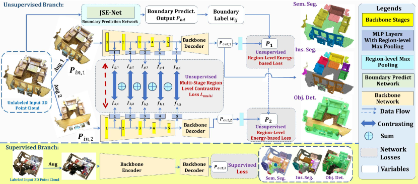
Energy Loss Guided by Boundary Labels. As shown in Fig. 3, we first perform data augmentation (detailed in the Appendix) for the input point clouds $\textbf{P}_{in}$ to obtain two transformed point clouds $\textbf{P}_{in,1}$ and $\textbf{P}_{in,2}\in\mathbb{R}^{N\times C_{in}}$, where N is the numbers of points. $C_{in}$ and $C_{out}$ are the numbers of input and output feature channels, respectively. Utilizing the backbone network SparseConv [59], we can obtain point cloud predictions $\textbf{P}_{out,1}$ and $\textbf{P}_{out,2}$. Then applying region-level max pooling on the same subregions, we obtain the predicted classes $\textbf{P}_{1}$, and $\textbf{P}_{2}\in\mathbb{R}^{M\times C_{out}}$ of the specific subregions. $\textbf{P}=\{p(s_{1}),p(s_{2}),...p(s_{i}),...,p(s_{R})\}$, where $R$ is the total number of regions obtained by over-segmentation. Denote the prediction of the $j_{th}$ neighboring region of the center region $s_{i}$ as $p(s_{i,j})$. Taking the unary network prediction and pairwise affinity between the neighbouring region into account, inspired by conditional random field (CRF) in DeepLab [29], we formulate the optimization energy function $E_{sum}$ as follows for label-efficient learning:

$$E_{sum}=\sum_{i}E_{i}(s_{i})+\sum_{i<j}^{adjacent}E_{i,j}(s_{i},s_{i,j}).$$ (8)

The first unary network prediction item $E_{i}(s_{i})$ is the entropy regularization term. It encourages region-level prediction with high confidence, which also facilitates the contrastive learning introduced subsequently, which is formulated as:

$$E_{i}(s_{i})=-log\,p(s_{i}).$$ (9)

We propose the pairwise affinity term of $E_{sum}$ as:

$$\begin{split}E_{i,j}(s_{i},s_{i,j})=H_{i,j}w_{i,j}[\epsilon-\|p(s_{i})-p(s_{i,j})\|]^{2}_{+}\\ +H_{i,j}(1-w_{i,j})\|p(s_{i})-p(s_{i,j})\|^{2}.\end{split}$$ (10)

$H_{i,j}$ is designed as the confidence indicator. $H_{i,j}=1$, if the probabilities which produce $p(s_{i})$ and $p(s_{i,j})$ are both larger than a threshold $\gamma$. Otherwise, it equals $0$. $\epsilon$ can be any value in the range of $(0,1)$. $p(s_{i})$ and $p(s_{i,j})$ are the semantic predictions for the $i_{th}$ center region and the $j_{th}$ neighbouring region, respectively. And $[x]_{+}$ is the maximum function $max(0,x)$. For adjacent boundary regions, we encourage their confident semantic or instance predictions to be different (i.e. larger $\|p(s_{i})-p(s_{i,j})\|$); while for the non-boundary adjacent regions, we force their semantic predictions to be the same (i.e. $\|p(s_{i})-p(s_{i,j})\|=0$). Different from the traditional energy function in DeepLab[29], which used handcrafted features to compare similarities, we propose to use the learned boundary region labels to guide the network’s confident max-pooled region-level predictions. Therefore, the proposed boundary-aware energy function better encourages semantic separations at boundaries. Furthermore, we only consider pairwise affinity between adjacent regions instead of all pixel pairs, which greatly reduces computation costs, and avoids noises induced by distant unrelated pairs in the meanwhile.

Figure 5: Qualitative instance segmentation results of proposed WS3D on ScanNet [20] with fully supervised state-of-the-art and the previous state-of-the-art GPC [121] in the 5% labeling ratio, compared with fully supervised arts. Different instances are indicated by different colors. And the intermediate over-segmentation results for obtaining regions and boundary predictions, with the boundary points indicated by the color blue.

3.2.2 Region-level Instance Discrimination

After applying the entropy regularization term $E_{i}(s_{i})$, we can obtain predictions at the region level with high confidence. Note that confident region-level predictions further improve the latent feature discrimination capacity of the network, which makes contrastive learning in the latent space feasible. Therefore, we further propose a multi-stage region-level contrastive learning for unlabeled data. Compared to previous work using only contrastive learning with low-level geometric registrations [27], our work unleashes potentials of contrastive learning with instance discrimination to enhance versatile feature learning in latent space.
The key to successful semantic/instance segmentation is maintaining discriminative feature representations at different stages of the backbone network [122]. Inspired by the pyramidal feature network [122, 123], we propose a simple but effective multistage contrastive learning approach for point clouds in an unsupervised setting. As shown in Fig. 3, given the augmented point clouds input $P_{in,1}$ and $P_{in,2}$, we feed them into the backbone encoder. We add five additional MLP heads with region-level max-pooling to obtain region-level segmentation predictions at the $m_{th}$ backbone stage, denoted as $\textbf{f}_{g,m}$ and $\textbf{f}_{h,m}$, respectively (five stages in our case, denote $M$ as the total network stages. i.e., $M$ = 5). After we apply the MLP heads to the extracted features at different stages, we can obtain the hierarchical feature embeddings of the fine-tuned downstream 3D scene understanding network. Unlike existing pixel-level [124], or point-level [124, 125] for point cloud contrastive learning, our proposed contrastive learning performs at the region level. Therefore, it will help to obtain more holistic regional information. The obtained regional information will be complementary to the point-level information. The region-level semantic contrastive loss is formulated as:

$$L^{m}_{contrast}=-\frac{1}{\textbf{S}_{p}}\sum_{(a,b)\in S_{p}}log\frac{H_{i,j}exp(\textbf{f}_{g,m}^{a}\cdot\textbf{f}_{h,m}^{+}/\tau)}{\sum_{(\cdot,c)\in S_{p}}H_{i,j}exp(\textbf{f}_{g,m}^{a}\cdot\textbf{f}_{h,m}^{-}/\tau))},$$ (11)

where $(a,b)\in\textbf{S}_{p}$ are latent confident predicted positive region pairs, and $(a,c)\in\textbf{S}_{p}$ are latent negative region pairs. As mentioned before, $H_{i,j}$ is designed to eliminate contrastive learning candidates with low confidence degrees. Reliable region-level contrastive learning is only applied to confident predictions by the network. After applying contrastive losses for instance discrimination, semantically similar features with high confidence levels in the latent space will become more adjacent, whilst semantically distinct ones will be separated, which will be shown in Fig. 13. Note that although a recent work GPC [121] has proposed methods to perform contrastive learning on the point clouds in a SSL manner, our work is different from their method in two aspects. Firstly, our contrastive learning is conducted at region level while GPC conducts contrastive learning at the point level. Secondly, GPC focuses on the selection of the positive and negative point-set samples to perform contrastive learning in a pseudo-label supervised manner on two different 3D scene samples, while we focus on the unsupervised contrastive learning which disentangles different feature representations in the latent space on the same augmented 3D scene sample, guided by confident network predictions, and it learns hirachical regional object information. 
The final proposed multi-stage contrastive learning loss is formulated as the sum of losses at every network stage:

$$L_{multi}=\sum_{m=1}^{M}L_{contrast}^{m},\vspace{-0.1mm}$$ (12)

After applying the multi-stage contrastive loss $L_{multi}$, the output at each stage of the network will provide more distinctive representations to attain better performance. From our ablation experiments, the performances can be boosted by applying multi-stage contrastive loss. We apply the typical self-training-based approach, where the high-confidence predictions are retained as the pseudo label for the network training in the subsequent iteration. We adopt the typical cross-entropy loss for the self-training which is denoted as $L_{ST}$. Considering $E_{sum}$ (see Eq. 8) for the two augmented scenes $P_{in,1}$, $P_{in,2}$, and $L_{multi}$ (see Eq. 12), we formulate the overall loss $L_{unlabeled}$ for the WS3D training with unlabeled data: $L_{unlabeled}=L_{ST}+\alpha E_{sum,2}+\beta L_{multi}$.

3.2.3 Supervised Learning for labeled data

We also guide network optimizations by using supervision from the labeled data. As shown in Fig. 3, we use the cross-entropy loss $L_{ce}$ to guide the supervised learning on the labeled data in the supervised branch. The loss term for the WS3D training with the labeled data is $L_{labeled}$. For the task of semantic segmentation, the loss for the labeled data $L_{labeled}$ includes the cross-entropy loss. For the backbone network selection, we follow previous work with the sparse convolutional network design for semantic [59] and instance segmentation [90], respectively. Our detection network is designed based on widely adopted VoteNet [126, 99]. We also use Dice [127] loss to guarantee tighter aggregations of points within the same cluster, and strict geometric separations of points in diverse clusters [99].

3.2.4 The Overall Optimization Loss Function

Leveraging our proposed region-level energy-based loss and region-level contrastive learning, the network can make maximum use of the unlabeled data for better feature learning to boost performance in the fine-tuning stage. As shown in Fig. 3, for semantic segmentation and instance segmentation, we fine-tune the network in an end-to-end manner for both supervised and unsupervised branches to make full use of labeled and unlabeled data. The weight value of the unsupervised loss is denoted as $\lambda_{u}$. The overall optimization function $L_{total}$ is formulated as follows, and we set $\lambda_{u}=2$ empirically:

$$L_{total}=L_{labeled}+\lambda_{u}L_{unlabeled}.$$ (13)

Figure 6: The captured 2D and 3D region proposals. It is demonstrated that more object proposals can be captured by our proposed combined unitive 2D/3D proposal generation approach.

Figure 7: The final ScanNet [20] object detection results. Differences in predictions are highlighted in the rectangles.

Figure 8: The object detection comparisons on KITTI [128] validation set. It can be demonstrated that our proposed WS3D++ provides very accurate bounding box predictions qualitatively compared with the previous state-of-the-art merely using 2D bounding boxes, which demonstrates the effectiveness of using 3D regional as well as 3D object-level information in facilitating effective feature representation learning.

Figure 9: Segmentation result comparisons with CLIP prompts for the indoor ScanNet benchmark. It can be seen from our results that clear object-level information can be captured with the designed visual prompts, which demonstrates the effectiveness of our designed hierarchical feature-aligned representation learning approaches.

4 Experiments

4.1 Pre-training Experimental Settings

For the indoor scene understanding tasks, we pre-train the network on ScanNet [20]. And for the outdoor scene parsing tasks, we pre-train the network on NuScenes [35] dataset. For the dataset partition, we follow the official partition of ScanNet-V2 [20] using 1,201 scans as the pre-training dataset. The NuScenes [35] is an outdoor autonomous driving dataset that contains 7000 training scenes, the dataset provides the camera’s intrinsic and extrinsic parameters, thus we can obtain the 2D to 3D transformations and alignments very easily from designed rendering approaches. For the indoor and outdoor pre-training, we pre-train the network for 500 epochs and then we fine-tune the network on diverse downstream tasks. The hyper-parameter $k$ in Top-$k$ is set to 3. The initial learning rate is set to $5\times 10^{-4}$ and is multiplied with 0.2 every 50 epochs.

4.2 Finetuning Experimental Settings

Datasets. During the fine-tuning, to demonstrate the effectiveness for both data-efficient learning and open-world recognition of the proposed WS3D and WS3D++ under the limited scene reconstruction labeling scheme, we have tested it on various benchmarks, including S3DIS [21], ScanNet [129], and SemanticKITTI [18] for semantic segmentation, and ScanNet [129] for instance segmentation, respectively. Detailed information on each dataset and training details are put into the Appendix.
Training Set Partition. Following the typical setting in data-efficient learning in the limited reconstruction case [22] [121], we partition the training set of all tested datasets into labeled data and unlabeled data with various labeling points percentage, e.g., {1%, 5%, 10%, 15%, 20%, 25%, 30%, 40%, 100%}. For the limited reconstruction case, noted that to partition the labeled points into a specific labeling ratio, we probably need to split a maximum of one scene into two sub-scenes. One of the sub-scenes belongs to the labeled data and the other sub-scene belongs to the unlabeled data.

TABLE I: Comparison of semantic segmentation results with different labeling percentages on ScanNet validation set, S3DIS validation set (Area 5), and SemanticKITTI validation set (Sequence 08). ’Sup-only-GPC’ denotes GPC model trained with only labeled data. ’WS3D’ denotes model trained with our proposed methods. We have shown the performance increase in the last row for each dataset, compared to merely trained models with labeled data (left value) and to the SOTAs GPC [121] (right value).

Datasets	Approaches	Semantic Segmentation mIoU (%) on the Validation Set According to Supervision Level (%)
		1%	5%	10%	15%	20%	25%	30%	40%	100%
ScanNet	Sup-only-GPC	40.9	48.1	57.2	61.3	64.0	65.3	67.1	68.8	72.9
	GPC [121]	46.6	54.8	60.5	63.3	66.7	67.5	68.9	71.3	74.0
	Mix3D [130]	47.1	55.2	61.1	63.5	66.8	67.9	68.7	71.5	73.3
	PointMixup [131]	44.5	55.2	69.6	63.7	66.3	66.9	68.8	70.2	73.8
	RDPL [132]	47.6	56.3	61.1	63.8	66.8	67.8	69.7	71.8	74.6
	Active-ST [133]	48.7	56.7	62.5	65.6	67.8	68.7	71.2	72.5	75.8
	WS3D [4]	49.9 +9.0	56.2 +8.1	62.2 +5.0	65.8 +4.5	68.5 +4.5	69.4 +4.1	70.3 +3.2	73.4 +4.6	76.9 +4.0
	WS3D++	52.6 +11.7	59.1 +11.0	65.2 +8.0	66.9 +5.6	71.8 +6.6	71.1 +5.8	72.6 +5.5	75.3 +6.6	81.7 +8.8
S3DIS	Sup-only-GPC	36.3	45.0	52.9	53.8	59.9	60.3	61.2	62.6	66.4
	GPC [121]	38.2	53.0	57.7	60.2	63.5	63.9	64.9	65.0	68.8
	Mix3D [130]	39.2	50.3	58.3	61.1	64.1	64.8	65.9	66.9	69.6
	WS3D [4]	45.3 +9.0	54.6 +9.6	59.3 +6.4	62.3 +7.0	65.7 +5.8	66.5 +6.8	67.2 +6.0	69.5 +6.9	72.9 +6.5
	WS3D++	48.6 +12.3	57.7 +12.7	61.2 +8.3	66.9 +11.6	70.6 +10.7	71.1 +10.8	72.6 +11.4	75.3 +12.7	81.7 +15.3
SemanticKITTI	Sup-only-GPC	28.6	34.8	43.9	47.9	53.8	55.1	55.4	57.4	65.0
	GPC [121]	34.7	41.8	49.9	53.1	58.8	59.1	59.4	59.9	65.8
	LESS [134]	37.1	42.5	50.5	53.9	59.5	59.6	60.5	63.5	66.9
	Mix3D [130]	37.7	42.9	50.8	54.1	59.9	60.9	61.8	61.3	68.8
	WS3D [4]	38.9 +10.3	43.7 +8.9	52.3 +8.4	55.5 +7.6	61.4 +7.6	61.8 +6.7	62.1 +6.7	63.2 +5.8	66.9 +1.9
	WS3D++	46.8 +18.2	58.6 +13.8	55.2 +11.3	62.8 +14.9	65.9 +12.1	67.9 +12.8	68.6 +13.2	70.9 +13.5	76.8 +11.8
Nuscene	Sup-only-GPC	39.8	45.9	47.1	48.6	55.7	56.3	58.9	59.8	67.9
	PRKT [135]	48.0	49.3	51.8	53.5	56.7	59.6	63.8	66.7	70.1
	SLidR [134]	48.2	50.3	52.9	55.8	56.9	59.1	60.8	63.8	66.9
	PointContrast [27]	48.3	50.2	55.1	58.1	60.2	61.1	62.1	64.9	69.2
	CLIP2Scene [27]	56.3	56.8	58.7	61.2	63.6	64.1	64.5	64.8	65.1
	LESS [134]	49.1	42.5	50.5	53.9	59.5	59.6	60.5	63.5	66.9
	Mix3D [130]	37.7	42.9	50.8	54.1	59.3	60.2	61.8	61.3	68.8
	WS3D [4]	49.1 +9.3	51.6 +5.7	52.3 +5.2	55.5 +6.9	61.4 +6.7	61.8 +5.5	62.1 +3.2	63.9 +4.1	71.6 +3.7
	WS3D++ [4]	53.7 +13.9	56.7 +10.8	55.2 +11.3	62.8 +14.9	71.6 +15.9	67.9 +11.6	68.6 +9.7	71.9 +12.1	77.8 +9.9

Figure 10: The final 3D scene-level activations results based on the language query of WS3D++. Better zoom in for details.

Implementation Details. For the task of semantic segmentation, we finetune the network for 500 epochs on a single NVIDIA 1080Ti GPU with a batch size of 16 during training. The initial learning rate is set to 1$\times$10^-3 and is multiplied with 0.2 every 50 epochs. We implement it in PyTorch and optimize it with Adam optimizer [136]. We set the hyperparameter $\gamma$ as 0.8 to ensure that merely highly confident prediction can be used for network optimization. $\epsilon$ is set to 0.5. We empirically choose $\alpha=\beta=1$, while $\lambda_{u}=0.1$. For instance segmentation, we train the network for 580 epochs on a single NVIDIA 1080Ti GPU with a batch size of 8 during training. The other settings are the same as the semantic segmentation task.

4.3 Data-efficient 3D Semantic Segmentation

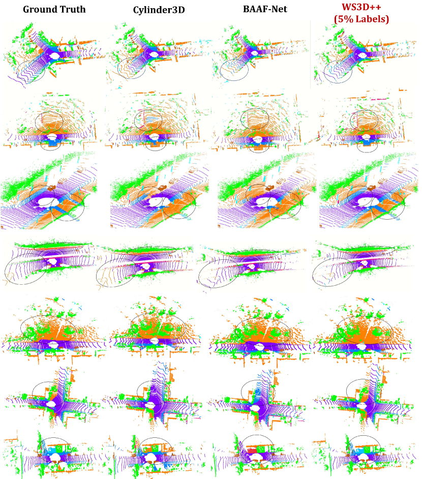
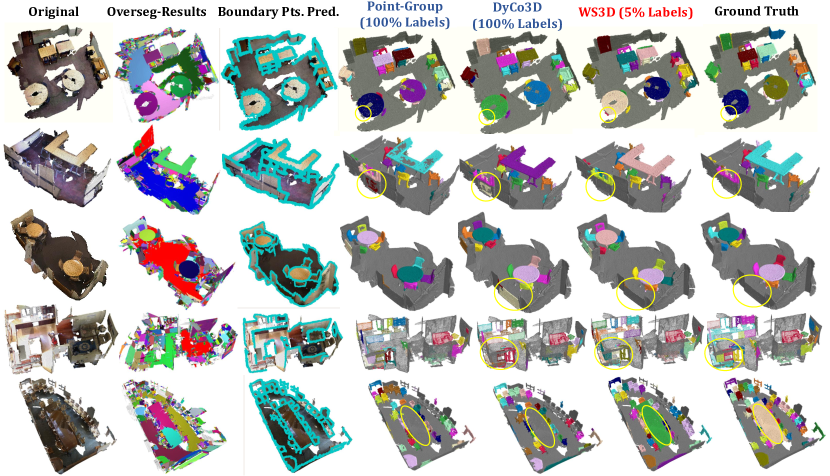
Overall Experimental Results. For the semantic segmentation, we have tested WS3D on versatile indoor and outdoor benchmarks, including ScanNet [20], S3DIS [21], and SemanticKITTI [18]. We have done extensive experiments with limited labeled data, e.g., only {1%, 5%, 10%, 15%, 20%, 25%, 30%, 40%, 100%} data in training set are available as labeled data. The qualitative results are shown in Fig. 4. In the meanwhile, the quantitative semantic segmentation performance is summarized in Table I. As mentioned, we have used the voxel-based method SparseConv [59] as the backbone. Our WSL model significantly surpasses the supervised-only model in GPC that is merely trained with labeled data, showing that our WSL can effectively make use of the unlabeled data to enhance the feature discrimination capacity of the model. Also, it can be observed the increment of performance is more obvious when the unlabeled data percentage is larger. For example, the performance increase on SemanticKITTI is 10.3% for the 1% labeling percentage, 5.8% for the 40% labeling percentage, and 1.9% for the 100% labeling percentage. This can be possibly explained by the fact that for more unlabeled data, our proposed WS3D can extract more meaningful semantic information from the unlabeled data based on our boundary-guided energy-based loss and confidence-guided region-level contrastive learning design. In addition, compared with current SOTA GPC, our proposed WS3D also achieves consistently better results in semantic segmentation performance, especially when faced with very limited label circumstances (e.g. 1% labeling points). In that case, WS3D outperforms GPC by 3.3%, 7.1%, and 4.2% for ScanNet, S3DIS, and SemanticKITTI, respectively. Fig. 4 shows that we can provide comparable performance compared with fully supervised SOTAs BAAF-Net [89] and Cylinder3D [119] on SemanticKITTI with 5% labels. As shown in Table I, the performance of our enhanced approach WS3D++ has remarkably increased performance compared with WS3D and previous SOTAs, demonstrating the effectiveness of our proposed vision-language knowledge-associated pre-training.

Figure 11: Segmentation result visualizations and comparisons with CLIP text encoder prompts for the outdoor KITTI benchmark. It can be demonstrated the foreground object awareness can be clearly captured comared with the previous SOTAs PLA [85]. Meanwhile, as shown in the last three columns, we can provide clear segmentation for the corresponding visual objects based on the textual prompts.

TABLE II: Comparison of experimental results on 20% and fully labeled case for the task of inductive and transductive learning for our proposed WS3D++, respectively. In transductive learning, the test set is also utilized for network training. We test the task of semantic segmentation on ScanNet, S3DIS, and SemanticKITTI with the evaluation metric of mIoU(%).

Datasets	20% label			100% label
	Base	Induct.	Transduct.	Base	Induct.	Transduct.
ScanNetv2-WS3D	64.0	68.5	71.4	72.9	76.9	77.6
ScanNetv2-WS3D++	67.3	73.9	75.6	77.3	80.3	81.6
S3DIS Area5 Val.	59.9	65.7	66.6	66.4	72.9	73.5
S3DIS WS3D	61.3	67.6	68.6	68.2	74.8	75.8
S3DIS WS3D++	62.8	68.9	69.9	69.7	75.5	76.9
Semantic KITTI Val.	53.8	61.4	64.5	65.0	66.9	68.2
Semantic KITTI Val. WS3D++	54.7	62.9	66.2	67.1	68.2	69.7
Semantic KITTI Test.	55.7	62.5	63.6	65.4	68.1	71.3
Semantic KITTI Test. WS3D++	56.6	63.7	65.3	67.1	69.7	72.8

TABLE III: Comparison of current State-of-the-art (SOTA) approaches in the limited reconstruction case for the 3D object detection tasks with different ratios of labeled data. The mean average precision (mAP) given by the mean $\pm$ standard deviation in three runs of diverse random splits are reported.

Datasets	Models	5%		10%		20%
		Induct.	Transduct.	Induct.	Transduct.	Induct.	Transduct.
SUN RGB-D [137, 66]	Baseline	29.9 $\pm$ 1.5	33.5 $\pm$ 0.8	34.4$\pm$ 1.1	40.7$\pm$ 0.9	41.1 $\pm$ 0.3	47.5 $\pm$ 0.5
	SESS [138]	34.2 $\pm$ 2.0	38.1 $\pm$ 0.7	42.9 $\pm$ 0.8	45.3$\pm$ 0.9	47.9 $\pm$ 0.4	51.6 $\pm$ 0.3
	3D-IOUMatch [139]	39.1 $\pm$ 1.9	46.3 $\pm$ 0.7	45.5 $\pm$ 1.5	53.5 $\pm$ 0.3	49.7 $\pm$ 0.5	54.3 $\pm$ 0.8
	SPD [140]	38.5 $\pm$ 0.7	44.3 $\pm$ 0.8	46.0 $\pm$ 1.0	51.7 $\pm$ 0.9	49.6 $\pm$ 0.5	54.5 $\pm$ 0.9
	WS3D (Ours)	46.9 $\pm$ 0.8	49.5 $\pm$ 0.7	47.8 $\pm$ 0.8	55.7 $\pm$ 0.8	55.6 $\pm$ 0.7	57.9 $\pm$ 1.2
	WS3D-Open (Ours)	47.8 $\pm$ 0.8	50.3 $\pm$ 0.6	49.3 $\pm$ 0.7	58.2 $\pm$ 0.7	59.1 $\pm$ 0.8	60.3 $\pm$ 1.1
	WS3D++ (Ours)	52.7 $\pm$ 0.7	54.5 $\pm$ 0.8	53.7 $\pm$ 0.9	63.8 $\pm$ 0.8	65.8 $\pm$ 0.7	65.6 $\pm$ 1.1
ScanNet-V2 [20]	Baseline	27.9 $\pm$ 0.5	30.8 $\pm$ 1.5	31.1 $\pm$ 0.7	33.2 $\pm$ 0.5	41.6 $\pm$ 0.9	44.5 $\pm$ 1.2
	SESS [138]	32.2 $\pm$ 0.8	36.8 $\pm$ 1.1	39.7 $\pm$ 0.9	44.5 $\pm$ 0.5	47.9 $\pm$ 0.4	49.2 $\pm$ 0.7
	3D-IOUMatch [139]	40.0 $\pm$ 0.9	46.3 $\pm$ 0.7	47.2 $\pm$ 0.4	49.6 $\pm$ 0.6	52.8 $\pm$ 1.2	54.3 $\pm$ 0.8
	SPD [140]	41.5 $\pm$ 0.5	44.3 $\pm$ 0.8	43.2 $\pm$ 1.2	46.2 $\pm$ 0.5	51.9 $\pm$ 0.5	55.1 $\pm$ 0.9
	WS3D (Ours)	45.8 $\pm$ 0.5	49.2 $\pm$ 0.6	47.7 $\pm$ 0.9	53.9 $\pm$ 0.6	55.6 $\pm$ 0.7	58.2 $\pm$ 1.3
	WS3D-Open (Ours)	47.2 $\pm$ 0.8	50.8 $\pm$ 0.6	51.1 $\pm$ 0.9	59.2 $\pm$ 0.8	59.0 $\pm$ 0.8	61.5 $\pm$ 1.6
	WS3D++ (Ours)	55.3 $\pm$ 1.1	57.6 $\pm$ 1.2	57.9 $\pm$ 0.8	65.8 $\pm$ 1.2	64.6 $\pm$ 0.5	66.5 $\pm$ 1.1

TABLE IV: Comparisons of the open vocabulary learning performance. It can be demonstrated that our proposed approach provides very superior open-world recognition performance compared with the diverse SOTAs. WS3D-Open abandons our feature-aligned contrastive pre-training with the contrastive loss term $\mathcal{L}^{total}_{Ctr}$ and directly uses the CLIP [9] feature encoder with the knowledge distillation loss term $\mathcal{L}^{Dist}_{\mathcal{KL}}$.

Datasets	Models	Few-shot settings
		B15/N4	B12/N7	B10/N9
ScanNet [20]	3DGenZ [141]	20.6/56.0/12.6	19.8/35.5/13.3	12.0/63.6/6.6
	3DTZSL [142]	10.5/36.7/6.1	3.8/36.6/2.0	7.8/55.5/4.2
	LSeg3D [139]	0.0/64.4/0.0	0.9/55.7/0.1	1.8/68.4/0.9
	PLA without caption [85]	39.7/68.3/28.0	24.5/70.0/14.8	25.7/75.6/15.5
	PLA [85]	65.3/68.3/62.4	55.3/69.5/45.9	53.1/76.2/40.8
	WS3D (Ours)	66.1/69.1/65.5	63.3/70.3/58.8	59.3/77.5/51.6
	WS3D-Open (Ours)	68.3/70.6/67.1	64.2/71.4/59.9	59.7/77.9/51.6
	WS3D++ (Ours)	72.3/69.1/73.3	73.3/70.0/63.6	65.2 / 78.9 / 58.8
	Fully-supervised	74.5/68.4/79.1	73.6/72.0/72.8	69.9/75.8/64.9
Datasets	Models	Few-shot settings
		B12/N3	B10/N5	B6/N9
NuScenes	3DGenZ [141]	01.6/53.3/00.8	01.9/44.6/01.0	01.1/52.6/00.5
	3DTZSL [142]	01.2/21.0/0.6	06.4/17.1/03.9	2.61/18.52/03.15
	LSeg-3D [85]	0.6/74.4/0.3	0.0/72.5/0.0	2.66/69.72/0.21
	PLA without caption [85]	25.5/75.8/15.4	10.7/76.0/05.7	8.95/65.83/6.32
	PLA [85]	47.7/73.4/35.4	24.3/73.1/14.5	15.63/60.32/12.38
	WS3D (Ours)	51.3/76.6/30.9	41.5/72.5/20.8	35.2/40.9/29.8
	WS3D-Open (Ours)	55.8/77.5/34.9	47.2/69.3/50.9	39.2/45.3/41.6
	WS3D++ (Ours)	58.6/79.1/38.6	49.7/67.3/53.9	40.6/46.6/51.9
	Fully-supervised	73.7/76.6/71.1	74.8/76.8/72.8	74.6/75.9/72.3

Figure 12: The WS3D++ corresponding detection and segmentation projections on six rendered 2D views through proposed multi-view rendering. It can be demonstrated that our proposed rendering has established an explicit modality association between the final 2D views and 3D views. Also, by combining 2D and 3D region proposals, more complete and apparent object-level information can be clearly captured both from 2D views and 3D views. Best zoom-in for viewing.

Figure 13: t-SNE visualization in semantic segmentation of the proposed WS3D under the 5% labeling percentage on S3DIS validation set. The diverse feature embeddings are indicated by different colors and are normalized into $[-1,1]$ for better visualization. It has been validated that more discriminative features can be acquired for diverse semantic classes with our proposed unsupervised region-aware fine-tuning strategy (demonstrated by WS3D) and our proposed hierarchical vision-language knowledge associated and distilled pre-training (demonstrated by WS3D++).

TABLE V: Comparison of the performance of instance segmentation, under various levels of supervision on ScanNet validation set. ’Sup-only-GPC’ denotes the model trained with only labeled data. ’WS3D’ denotes the model trained with our proposed methods. In the last row, we have shown the performance increase of WS3D. WS3D-Open abandons our feature-aligned contrastive pre-training with the contrastive loss term $\mathcal{L}^{total}_{Ctr}$ and directly uses the CLIP [9] feature encoder with the knowledge distillation loss term $\mathcal{L}^{Dist}_{\mathcal{KL}}$.

Tested Dataset	Approaches	Ins. Seg. Results with the metric of AP@50%
		1%	5%	10%	15%	20%	30%	35%	40%	100%
ScanNet	Sup-only-GPC [121]	10.8	33.6	42.8	45.3	48.2	49.0	49.5	50.2	56.8
	Mix3D [130]	12.7	34.7	43.1	45.7	48.7	49.6	50.2	51.3	57.6
	GPC [121]	16.9	38.6	44.9	47.2	48.6	49.7	51.2	52.0	57.7
	SPIB_Ins [143]	17.1	38.9	45.3	47.9	48.9	50.5	51.6	52.7	57.6
	WS3D (Ours) [4]	30.8	45.6	53.5	54.7	53.2	51.9	52.5	53.0	58.7
	WS3D-Open (Ours)	31.2	50.6	55.8	57.9	56.8	58.7	58.9	59.5	65.1
	WS3D++ (Ours)	39.2	54.8	57.3	58	+8.6	+9.7	+9.4	+9.3	+8.3

4.4 Data-Efficient 3D Instance Segmentation

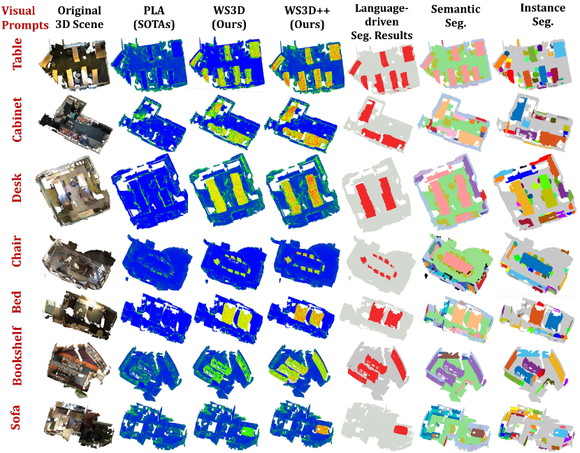
As our method can be integrated seamlessly into various network backbones and applied to different highly-level understanding tasks, we have also integrated our method with Point-Group [90] for the instance segmentation on ScanNet with results shown in Table V. Notice that the performance increase is 21.7% when merely 1% data is labeled compared with the sup-only case. It further demonstrates that our proposed approaches for the unsupervised branch have effectively exploited the unlabeled data to improve the feature learning capacity of the model. As shown in Fig. 5, our proposed WS3D and WS3D++ both provide explicit boundary guidance for separating diverse kinds of semantic classes, and the instance segmentation performance with very limited labeling percentage is comparable to those fully supervised counterparts.

4.5 Data-Efficient 3D Object Detection

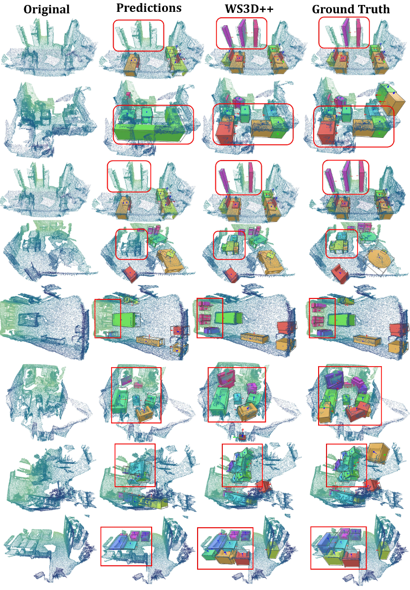
For the data-efficient 3D object detection, following our previous work [99], we evaluate current approaches extensively on SUN RGB-D [137] and ScanNet [20] benchmarks for 3D object detection tasks with the strong 3D object detection backbone VoteNet [126]. It can be demonstrated the open-vocabulary designs can to some extent boost the 3D object detection performance, which demonstrate the generalization capacity of our fundation model. As shown in Table III, we have also tested the ablated approach WS3D-Open which abandons our feature-aligned pre-training term $\mathcal{L}^{total}_{Ctr}$ and directly uses the CLIP [9] feature encoder for the knowledge distillation loss term with $\mathcal{L}^{Dist}_{\mathcal{KL}}$. It can be demonstrated that the performance degradation can obviously be observed when comparing WS3D-Open to WS3D, which demonstrate the effectiveness of our proposed hierarchical feature aligned pre-training in improve data efficiency.

TABLE VI: WS3D and WS3D++ ablation studies on ScanNet (Left Value), S3DIS (Middle Value) and Nuscene (Right Value) validation set, for semantic segmentation (Metric: mIoU%) and on ScanNet validation set for the instance segmentation (Metric: AP@50%), both tested with the 5% labeled case.

Cases	Base	$w_{i,j}$	$H_{i,j}$ in EF	$H_{i,j}$ in UCSL	UCSL	MS-UCSL	SCE	WS3D mIoU%	WS3D++ mIoU%	WS3D AP@50%	WS3D++ AP@50%	WS3D mAP%	WS3D++ mAP%
No. 1	✓	✓	✓	✓		✓	✓	56.2 / 54.6 / 53.9	62.8 / 58.1 / 56.3	45.6	54.8	45.8	58.9
No. 2	✓		✓	✓		✓	✓	51.0 / 49.3 / 47.8	57.1 / 52.5 / 50.9	39.9	48.5	40.6	53.6
No. 3	✓			✓		✓	✓	49.9 / 47.2 / 46.6	53.1 / 50.9 / 47.9	37.0	44.5	38.1	51.7
No. 4	✓	✓		✓		✓	✓	51.6 / 52.1 / 47.9	56.1 / 54.8 / 47.7	40.1	46.7	41.6	51.5
No. 5	✓	✓	✓			✓	✓	51.1 / 51.4 / 49.6	57.1 / 53.8 / 49.8	40.7	47.6	40.8	53.6
No. 6	✓	✓	✓	✓	✓		✓	52.5 / 50.9 / 50.3	56.7 / 53.9 / 49.5	42.2	48.7	39.8	53.8
No. 7	✓	✓	✓				✓	49.3 / 48.0/ 47.6	55.6 / 53.5/ 50.8	38.1	46.8	39.8	54.3
No. 8	✓	✓	✓	✓		✓		54.3 / 52.8 / 50.8	60.6 / 55.3 / 52.7	42.9	48.1	41.2	52.7
No. 9	✓						✓	48.1 / 45.3 / 45.7	50.8 / 47.6 / 50.6	34.8	39.8	33.9	45.3

TABLE VII: Ablation studies of the designed models of our proposed WS3D++. It is demonstrated that the proposed proposal generation approach and local and global contrastive approach can significantly boost final recognition performance.

Cases	2D Proposal	3D Proposal	$\mathcal{L}^{G}_{Ctr}$	$\mathcal{L}^{L}_{Ctr}$	mIoU%	AP@50%	ScanNet B10/N9	Nuscene B6/N9
No. 1	✓	✓	✓	✓	62.7 / 58.1 / 56.3	58.5 / 55.6 / 53.7	65.2 / 78.9 / 58.8	69.7 / 71.7 / 66.8
No. 2	✓		✓	✓	55.2 / 51.9 / 50.6	51.3 / 48.8 / 47.9	56.9 / 70.7 / 53.8	66.1 / 66.6 / 64.5
No. 3		✓	✓	✓	53.6 / 50.6 / 49.6	52.6 / 48.5 / 47.6	52.6 / 48.5 / 47.6	53.6 / 48.5 / 47.6
No. 5	✓	✓		✓	53.2 / 51.7 / 49.3	50.2 / 46.1 / 45.8	50.8 / 45.8 / 45.5	50.8 / 46.7 / 45.8
No. 6	✓	✓	✓		51.2 / 49.2 / 49.1	49.2 / 45.8 / 45.2	48.8 / 44.7 / 44.2	48.2 / 43.8 / 43.2

4.6 Ablation Study

Ablations: The results for WS3D are summarized in Table VI. We have ablated network modules in all combinations of settings as follows. Take the ScanNet instance segmentation at AP@50% as examples: Case 1: The full WS3D. Case 2: Removing the boundary prediction network, and not using the guidance of $w_{i,j}$. The framework still consists of the supervised branch, unsupervised guidance of the energy function based on the predicted confident pseudo label, and contrastive learning. This setting leads to a significant drop of 5.7% on AP. Case 3: Removing the pairwise term in the energy-based optimization function $E_{sum}$, the AP drops largely by 8.6%. Case 4: Removing $H_{i,j}$ in the energy function, the performance drops by 5.5%. Case 5: Removing $H_{i,j}$ in the unsupervised contrastive learning, the performance drops by 4.9%. Case 6: Conducting contrastive learning only with the region-level feature $\textbf{f}_{g,5}$ and $\textbf{f}_{h,5}$ at the fifth network stage, rather than at multiple stages. The performance drops by 3.4%. Case 7: Removing the unsupervised region-level contrastive learning branch, the performance drops largely by 7.5%. Case 8: Removing the supervised learning branch with the cross-entropy loss, the performance drops by 2.7%.

The results for WS3D++ are summarized in Table VII. Case 9: Only using the supervised branch, the ins. seg. performance drops significantly by 10.8%. Case 10: As demonstrated in Table VII, dropping the 2D or 3D proposals will both result in the performance drops both for the semantic segmentation as well as instance segmentation. Case 11: As shown in Table VII, either removing the global contrastive loss or the local contrastive loss results in less effective contrastive representations and affects the final downstream scene understanding performance.

Analyses: From the above ablations, some important findings are summarized: For WS3D, firstly, not using our designed modules results in a significant performance drop (Cases No. 3, No. 7, and No. 9), which demonstrates the effectiveness of the proposed unsupervised branch and learning strategies to leverage the unlabeled data. Secondly, our proposed learning strategies with boundary label $w_{i,j}$ (Case No. 2), energy function design (No. 3), high-confidence prediction based energy function design (No. 4), high-confidence based region-level contrastive learning strategy (No. 5), multi-stage contrastive learning network design (No. 6), all have a boost on the overall semantic/instance segmentation performance. The results demonstrate that the proposed energy loss is significant for semantic/instance seg. performances, because semantic boundary labels are crucial for identifying diverse objects. Thirdly, removing the supervision (Case No. 8), our method still maintains performance with a slight drop of performance by 2.7%. It further validates the robustness and feature learning capacity of our approach. Last but not least, as demonstrated in Table VII, for our proposed WS3D++, either dropping the 2D/3D proposals, or dropping the global/local contrastive loss result in considerable performance drops. It validates the effectiveness of our designs in enhancing discriminative 3D representations.

4.7 Qualitative and Quantitative Results of the Open-world Recognition Approaches

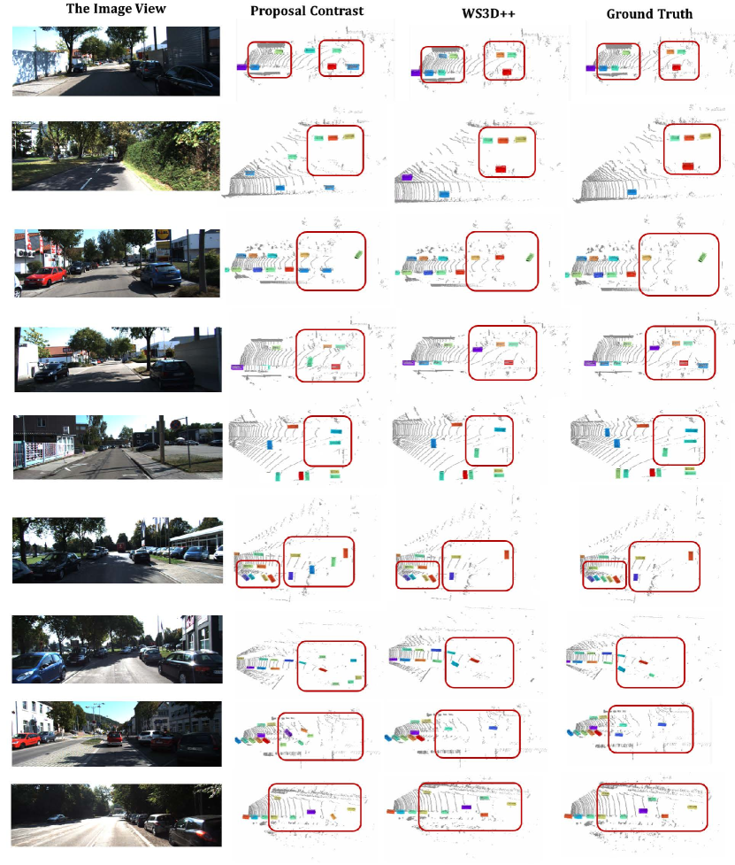
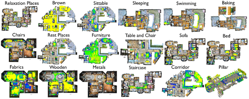
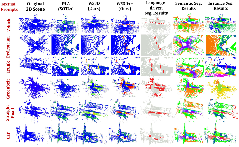
In this Subsection, we further evaluate the performance of the open-world recognition capacity of our proposed approach. The results of open-world recognition are shown in Table IV. We have compared our work with the previous approach PLA [85] in establishing the sufficient point-language associations for the open-world robot learning. The results demonstrate that our proposed approach has superior performance in open-world recognition. We directly use the settings in the PLA [85] and split the categories on ScanNet [20] and Nuscene [35] into base and novel categories. It can also be validated that WS3D-Open, which abandons our feature-aligned pre-training and directly use the CLIP [9] feature encoder, provides slightly inferior performance compared with WS3D++, validating the effectiveness of our language-3D matching strategy designs. WS3D++ exhibits superior performance in terms of the open-vocabulary few-shot learning for diverse partitioning of original and novel classes. The open-world recognition results are shown in Figure 9 and Figure 11. It can be demonstrated that better foreground object awareness can be effectively capture by our proposed WS3D++ compared with PLA [85], with superior segmentation performance guided by the textual prompts. The superior open-world recognition performance can be achieved while conducting open-world learning in diverse spliting of based and novel classes, including B15/N4, B12/N7, B10/N9 for the ScanNet [20] as well as B12/N3 and B10/N5 for the NuScenes [35]. It demonstrates robustness of our proposed approach. Also, as demonstrated in Figure 10, the WS3D++ language driven-3D scene segmentation results are very precise as shown qualitatively, which is corresponding to the object queried by the language, and it demonstrates that the inference can be done based on the object, material, properties, affordance, room type, etc. It demonstrates that our proposed WS3D++ can enable the scene-level object recognition based on the semantic language queries. As further shown in Figure 12, through our effective rendering techniques, which establish the explicit 2D-3D association, the aligned representation of 2D-3D-language co-embeddings can be learned and the objectness can also be enhanced through finding the similarity among diverse views through contrastive learning approaches. Also, by combining 2D and 3D region proposals, more complete and apparent object-level information can be clearly captured both from 2D views and 3D views.

4.8 Instance Discrimination Capacity

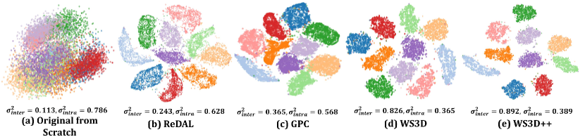
We show t-SNE visualizations of the learned latent feature representations for various semantic classes in Fig. 13. The case study task is the semantic segmentation on the S3DIS dataset with a supervision level of 5%. It is demonstrated that more distinctive and better separated point-wise feature embeddings are provided by our proposed unsupervised region-level contrastive learning, which can be attributed to its strong instance discrimination capacity. And more separated feature space can be provided with our proposed WS3D++ compared to WS3D and GPC. This strong instance discrimination capacity can be explained by more discriminative feature representations guided by 3D vision-language aligned representations, and is thus more beneficial to high-level semantic and instance segmentation performances both in terms of data efficiency and open-world recognition capacity. Also, our proposed hierarichical feature alignment also provides more separated feature space, which means that the feature alignment successfully enhances the final instance discrimination capacity.

5 Conclusion

In this paper, we proposed a general WS3D++ framework for data-efficient 3D scene parsing. It involves both the pre-training and the fine-tuning stages. In the pre-training stage, we propose the hierarchical feature alignment strategy to acquire accurate regional 3D-linguistic pairs, thus the performance can be enhanced to a large extent. At the same time, we propose an unsupervised boundary-aware energy-based loss and a novel region-level multi-stage semantic contrastive learning strategy, which are complementary to each other to make the network learn more meaningful and discriminative features from the unlabeled data. The effectiveness of our approach is verified across three diverse large-scale 3D scene understanding benchmarks under various experiment circumstances. Our approach can maximally exploit the unlabeled data to enhance the performance both for 3D point clouds semantic segmentation and instance segmentation, under various labeling percentages in the limited reconstruction case. Our proposed label-efficient learning framework, termed WS3D++, provides conprehensive baselines for future 3D scene parsing methods when the label is inaccessible or limited.

Robot Arm Grasping Example

We deploy our approach for the task of open-world perception in robot grasping. We use our proposed approach for segmentation and use the ROS 2 Gazebo-based framework to implement the other components of the system, such as kinematics/dynamics modeling, motion planning, low-level control, point cloud-based pose estimation, etc. Our proposed approach has robust performance and decent accuracy in grasping, which demonstrates the potential of our proposed WS3D++ in industrial manipulation applications in grasping and dropping novel objects beyond the training set. The video demos are attached.

Kangcheng Liu is currently an assistant professor at The Hong Kong University of Science and Technology (Guangzhou), and a joint assistant profesor at The Hong Kong University of Science and Technology. Before that, he was a senior robotics engineer and research fellow at Nanyang Technological University, Singapore, and served as the technical lead of several governmental and industrial projects in Hong Kong and Singapore. He received his B.Eng. degree from the Harbin Institute of Technology and his Ph.D. degree in robotics from the Chinese University of Hong Kong. His interests are robotic systems, vision and graphics, computational design, and manufacturing automation. He has been nominated to serve as the program committee member of international flagship conferences: ICRA, ICPR, ICIP, and CASE. He has published more than 40 international journal and conference papers with wide first-authored publications in TOP-Tier venues including IJCV, IEEE T-MECH, IEEE T-PS, IEEE T-CYB, IEEE T-IE, IEEE T-IP, IEEE T-ITS, CVPR, ECCV, ICCVW, RSS, ICRA, IROS, ACM MM, CBM, and among others as the first author or the corresponding author. He also served as the reviewer of more than 40 kinds of international journals and conferences such as IJCV, T-PAMI, T-RO, T-CYB, JFR, AIJ, IJRR, CVPR, ICCV, ECCV, TOG, and ACM SIGGRAPH. He is a member of IEEE and ACM.

Kai Tang is currently a professor at The Hong Kong University of Science and Technology, Guangzhou. He received the B.E. degree in mechanical engineering from the Nanjing Institute of Technology, China, in 1982, and the Ph.D. degree in computer engineering from the University of Michigan, Ann Arbor, USA, in 1990. From 1990 to 2001, he was at CAD/CAM Software Industry, USA. Since June 2001, he has been a Faculty Member with The Hong Kong University of Science and Technology, Hong Kong, where he is a Professor with the Department of Mechanical and Aerospace Engineering. His current research interests include multi-axis machining and additive manufacturing.

Yong-Jin Liu received the B.Eng. degree from Tianjin University, Tianjin, China, in 1998, and the M.Phil. and Ph.D. degrees from The Hong Kong University of Science and Technology, Hong Kong, China, in 2000 and 2004, respectively. He is currently a Professor with the BNRist, MOE-Key Laboratory of Pervasive Computing, Department of Computer Science and Technology, Tsinghua University, Beijing, China. His research interests include computational geometry, computer vision, cognitive computation, and pattern analysis. For more information, visit https://cg.cs.tsinghua.edu.cn/people/ Yongjin/Yongjin.htm

Ming Liu received the B.A. degree in automation from Tongji University, Shanghai, China, and the Ph.D. degree from the Department of Mechanical Engineering and Process Engineering, ETH Zurich, Zurich, Switzerland. He was a Visiting Scholar with the University of Erlangen-Nuremberg, Erlangen, Germany, and the Fraunhofer Institute of Integrated Systems and Device Technology, Erlangen. He is currently an Associate Professor with the The Hong Kong University of Science and Technology, Guangzhou. His research interests include robotics and autonomous systems, with prominent contributions in autonomous localization and mapping, visual navigation, semantic topological mapping, and environment modeling.

Baoquan Chen is currently an Endowed Boya professor with the National Key Lab of Genaral AI, Peking University, where he is the Associate Dean of the School of Artificial Intelligence. He received the MS degree in electronic engineering from Tsinghua University, Beijing, China, and the 2nd MS and PhD degrees in computer science from the State University of New York at Stony Brook, New York, USA. His research interests generally lie in computer graphics, computer vision, visualization, and human-computer interaction. He has published more than 200 papers in international journals and conferences, including 40+ papers in ACM Transactions on Graphics (TOG)/SIGGRAPH/SIGGRAPH-Asia. Chen serves/served as associate editor of ACM TOG/IEEE Transactions on Visualization and Graphics (TVCG), and has served as conference steering committee member (ACM SIGGRAPH Asia, IEEE VIZ), conference chair (SIGGRAPH Asia 2014, IEEE Visualization 2005), program chair (IEEE Visualization 2004), as well as program committee member of almost all conferences in the visualization and computer graphics fields for numerous times. For his contribution to spatial data visualization. He was inducted to IEEE Visualization Academy.

Supplementary Material

In this supplementary material, additional experimental results and details that are not included in the main paper due to space limits are provided as follows:

• Details of our experimental datasets (see Section A).

• Additional qualitative experimental results (see Section B).

• The PFH-based point cloud over-segmentation method to provide the initial over-segmentation results for our proposed WS3D (see Section C).

• Details of our data augmentation approach (see Section D).

• Training details of the boundary prediction network (see Section E).

• The low density issues for the outdoor point clouds captured by LiDAR sensors (see Section F).

A Experimental Datasets Details

To demonstrate the effectiveness of our proposed WS3D and WS3D++, we tested it on both indoor and outdoor 3D scene segmentation benchmarks, including S3DIS[21], SemanticKITTI[18], and ScanNet[20] for semantic segmentation, and ScanNet[20] for instance segmentation. The detailed information of each dataset is listed as follows:

Figure 14: Qualitative semantic segmentation results on SemanticKITTI with 5% labels, compared with the fully-supervised arts Cylinder3D [119], and BAAF-Net [89] with semantics indicated by diverse colors. The red circles highlight the performance difference between diverse methods.

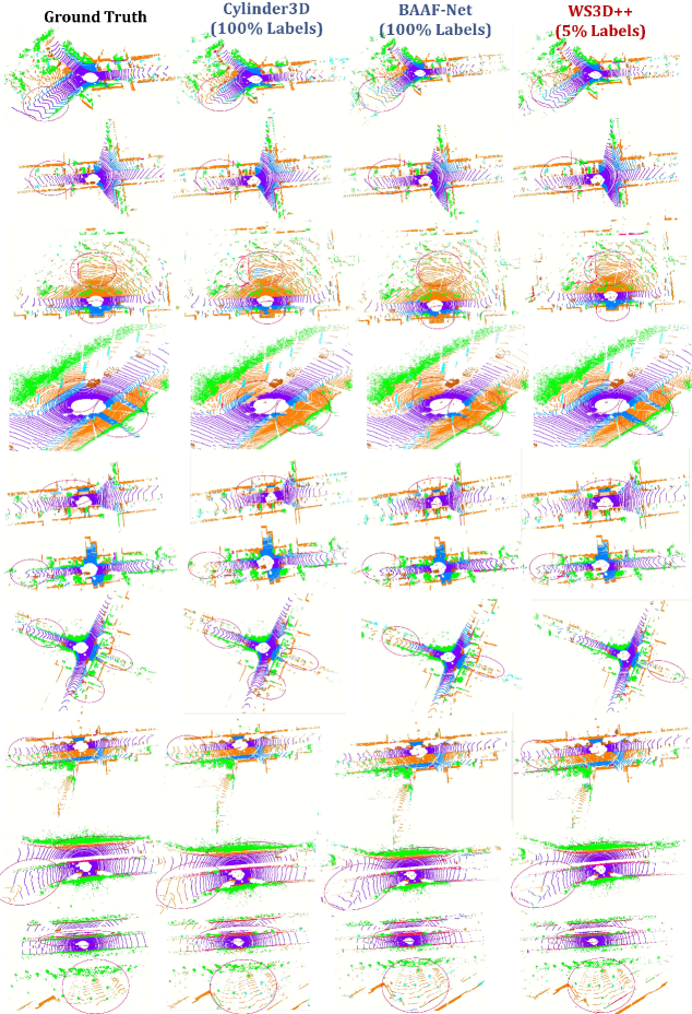
ScanNet-V2 is a standard large-scale and widely-acknowledged 3D indoor scene understanding benchmark consisting of more than 1,600 3D scene scans. It contains densely reconstructed point clouds from RGB-D images captured by the depth camera. For the dataset partition in fully supervised learning, we follow the official partition of ScanNet-V2[20] using 1,201 scans as the training set, 312 scans as the validation set, and 100 scans as the test set.

SemanticKITTI[18] is a large-scale point cloud understanding benchmark for self-driving applications. The point cloud of individual scenes is obtained densely by Velodyne VLP-64 LiDAR. The dataset covers long-range road scenes, thanks to the vehicle driving in complex road scenarios with mounted LiDAR to capture the point clouds. More than 43,550 labeled LiDAR scans in total are split into 21 sequences. Each LiDAR scan contains approximately $10^{5}$ points. We follow the official setting[18] that uses the sequences 00 to 07, and 09 to 10 for training, the sequence 08 for validation, and the sequence 11 to 21 for testing.

S3DIS is a commonly used indoor 3D scene understanding benchmark that contains various indoor scenes. It includes six indoor areas which are made up of 271 rooms. Each room contains a magnitude of $10^{6}$ points. The typical room size is $20\times 15\times 5$ meters. In our experiments, we follow GPC[121] using area 5 as the validation set and the other areas as the training set.

NuScene is a commonly used autonomous driving dataset containing more than 1000 scenes. Every scene is elaborately annotated with the 3D bounding boxes for 23 categories and 8 attributes. For the base/novel category partition, we overlook the ’otherflat’ class and randomly divide the rest 15 classes into B12/N3 and B10/N5 as in PLA [85].

Figure 15: Results of our proposed PFH-based over-segmentation in Algorithm 1. Diverse over-segmented regions are indicated by diverse colors.

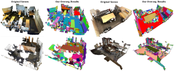
B Additional Experimental Results

We provide the additional experimental qualitative results on ScanNet and SemanticKITTI semantic segmentation and ScanNet instance segmentation.

In Fig. 14, the results on SemanticKITTI[18] are shown for the 5% labels case compared with the fully-supervised SOTAs Cylinder3D[119], and BAAF-Net[89]. From the qualitative results, our method can sometimes offer better segmentation performance than fully-supervised SOTAs for objects such as roads, trees, etc., which demonstrates the effectiveness of our proposed WS3D for outdoor 3D semantic segmentation.

Comparisons with SOTAs in the fully supervised mode. To demonstrate the feature learning capacity of our proposed WS3D, we have also experimented with the 100% labeling percentage for a fair comparison with fully supervised SOTAs. The results are shown in Table VIII and the last column of Table I. We have fed the whole training set into the supervised branch and unsupervised branch in Fig. 3 simultaneously. Therefore, our proposed energy-based loss and region-level contrastive learning strategy operate as additional optimization guidance for network training. Table VIII demonstrates that we can realize at least comparable or even better results, compared with the fully supervised SOTAs.
Transductive learning. Similar to the experimental setting of [121], we have also conducted experiments evaluating the performance of WS3D in transductive learning. Different from the inductive learning we tested above that requires the trained model to be generalized to an unseen test set, transductive learning can exploit the testing set when training. Compared with inductive learning, we add the test set as part of the unlabeled data in transductive learning. As is demonstrated in Table III, the sem. seg. mIOU becomes higher if the network is learned in a transductive way, both for the fully labeled case with 100% labels and the weakly labeled case with 20% labels. It demonstrates that our proposed WSL approaches, including the energy-based boundary-aware loss and the region-level contrastive learning, can leverage the unlabeled data for feature learning effectively in an implicit way to enhance the final segmentation performance.

Figure 16: In the limited reconstruction case, our proposed approaches WS3D and WS3D++ work well for the low-density SemanticKITTI over-segmentation and boundary prediction (5% label percentage). It can also be demonstrated that the explicit boundary information can be clearly captured, and our proposed approach is robust to the density variation of indoor dense and outdoor sparse point clouds.

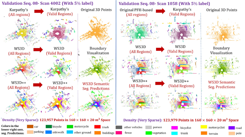
C Point Clouds Over-segmentation

C.1 PFH-based Point Clouds Over-segmentation

As mentioned in Subsection 3.1 in the main paper, the previous over-segmentation methods depended on the region growing[34], which relied heavily on the accurate normal estimation and were easily influenced by noises. In our work, we use the normal, curvature, and point feature histogram[116] simultaneously to provide the initial over-segmentation results for obtaining different regions. The point feature histogram (PFH)[116] can be regarded as a robust representation of local geometric features, which is robust to 6D pose transformation and deals well with diverse sampling densities, and neighboring noises. We use it as a more robust geometric feature to obtain the over-segmentation result.

To be more specific, we denote the average normal vector of a point as $\textbf{n}=(n_{x},n_{y},n_{z})$, the PFH feature as $\textbf{f}_{pfh}\in\mathbb{R}^{125\times 1}$. The cosine of the angle between the average normal vectors of two adjacent points $P_{i}$ and $P_{j}$ is denoted as $A_{n}$, and the cosine of the angle between two PFH vectors of two adjacent points in the 125-dimensional space is denoted as $A_{pfh}$. The Affinity $A(P_{i},P_{j})$ of two adjacent points $P_{i}$ and $P_{j}$ is given as:

$$A(P_{i},P_{j})=\sqrt{A_{n}^{2}+A_{pfh}^{2}}.$$ (14)

According to the Point Cloud Library (PCL)[34], in the process of region growing, points with an affinity larger than a threshold $T_{thres}$ are merged iteratively. We set $T_{thres}$ as 1 following the typical setting[34]. As shown in Algorithm 1, we summarize the detailed procedures for the PFH-based over-segmentation as the following steps:

Input: The input raw point set $\textbf{P}_{i}=\{p_{i}\},i=1,2,...,N_{i}$. $p_{i}=(x_{i},y_{i},z_{i})$.

Output: The output pseudo label matrix $\textbf{{L}}_{region}$ for different regions.

Initialize $P_{seed}=p_{\{seed,i\}},i=1,2,...,N^{seed}$;

Initialize the pseudo label matrix $\textbf{{L}}_{region}$ as a zero matrix.

while not converged do

       Select $K$ nearest neighbour points $p_{j}$ around the seed points $p_{seed}$ for comparisons based on fast Octree-based $K$ Nearest Neighbour search;

      

      for the seed points $p_{j}$ selected do

             if Condition 1 then

                  Assign $p_{j}$ the same overseg-label as $p_{seed}$;

                   if Condition 2 then

                        Regard the point $p_{j}$ as new seed points;

                  

            else

                  Assign $p_{j}$ with a new overseg-label. Regard $p_{j}$ as new seed points;

            $j\leftarrow j+1$;

            

            Update the pseudo label matrix $\textit{{L}}_{region}$.

      

return The class label matrix $\textit{{L}}_{region}$ of $\textbf{P}_{i}$ with different clusters.

Algorithm 1 The Proposed PFH-based Region Growing Over-segmentation to Obtain Regions

1. Select the points that have top 2‰ minimum curvatures[34] as the initial seed points $p_{seed}$. Utilizing fast $K$ Nearest Neighbour search[120], we obtain the $j_{th}$ neighbouring point $p_{j}$ of the initial seed point $p_{seed}$, and calculate the Affinity $A(p_{seed},p_{j})$ between $p_{seed}$ and $p_{j}$.

2. If the Affinity $A(P_{seed},P_{j})$ is larger than $T_{thres}$ (Condition 1), we assign the $j_{th}$ neighbouring point $p_{j}$ with the same label as $p_{seed}$.

3. If Condition 1 is satisfied, denote the curvature of $p_{j}$ and $p_{seed}$ as $r_{j}$ and $r_{seed}$, and denote the difference of $r_{j}$ and $r_{seed}$ as $\Delta r=\|r_{j}-r_{seed}\|$. If $\Delta r\leq\sigma$ (Condition 2), we set $p_{j}$ as the seed point. That means we set the points $p_{j}$ as seed points, only if the difference in curvature is small enough. Otherwise, we only assign $p_{j}$ the same label as $p_{seed}$.

4. If Condition 1 is not satisfied, we assign the neighbouring point $p_{j}$ with a different label from $p_{seed}$, and also assign $p_{j}$ as the seed point.

Finally, points are assigned to initial over-segmented regions with labels. The simple algorithm is summarized in Algorithm 1. The loop will terminate if any one of the following convergence conditions is satisfied, which are proposed:

1. All points have been assigned with labels;

2. There are no seed points that can be added.

After the procedures above, we can obtain the label $\textit{{L}}_{region}$, which indicates the separated regions obtained by over-segmentation. Some randomly selected over-segmentation results are shown in Fig. 15. The PFH-based over-segmentation can automatically divide the whole point cloud scene into geometrically separated regions as shown in Fig. 15. Different colors indicate different regions.

TABLE VIII: Comparison of SOTAs methods in the semantic segmentation performance on ScanNet validation set, S3DIS validation set (Area 5), and on SemanticKITTI validation set and test set. All results are based on the 100% label ratio. Top-two results are highlighted.

Approaches	Venue	ScanNet	S3DIS	SemanticKITTI
		Val.	Val. (Area 5)	Val.	Test
Minkow-Network [37]	CVPR19	72.2	65.4	61.1	63.1
PointASNL [49]	CVPR20	66.4	62.6	-	58.8
KPConv [144]	ICCV19	69.2	67.1	-	46.8
SPV-NAS [145]	ECCV20	-	-	64.7	66.4
Fusion-Net	ECCV20	-	67.2	63.7	61.3
MV-Fusion [44]	ECCV20	76.4	65.4	-	-
Cylinder3D [119]	CVPR21	-	-	65.9	67.8
BAAF-Net [89]	CVPR21	-	72.1	61.2	59.9
Sup-only-GPC [121]	ICCV21	70.9	66.4	65.0	65.4
GPC [121]	ICCV21	74.0	68.8	65.8	67.7
WS3D	ECCV22	76.9	72.9	66.9	69.0
WS3D++	-	77.6	73.5	67.7	69.8

D Data Augmentation Details

D.1 Data Augmentation Approaches

We perform three kinds of data augmentations to enhance the unlabeled data and to perform region-level contrastive learning, including: 1. Geometric rotations and mirroring of the point cloud scene. 2. Adding minor disturbance to the point cloud scene. 3. Random scaling of the point cloud scene.

Geometric rotations and mirroring. The original point cloud scene $\textit{P}\in\mathbb{R}^{N_{p}\times(3+f_{a})}$ can be partitioned into the coordinate channels of point clouds 3D positions $P_{x}\in\mathbb{R}^{N_{p}\times 3}$ and the feature channels $P_{f}\in\mathbb{R}^{N_{p}\times f_{a}}$ with diverse attributes such as the color and normal. We perform rotation of the point clouds around the X axis. Denote the rotated point clouds as $P_{x}^{r}$, and the rotation matrix as $R_{x}$, we can obtain the transformed point clouds as: $P_{x}^{r}=P_{x}R_{x}$, where $R_{x}=\begin{gathered}\begin{bmatrix}1&0&0\\ 0&cos(\phi)&-sin(\phi)\\ 0&sin(\phi)&cos(\phi)\end{bmatrix}\quad\end{gathered}$. $R_{x}$ is the rotation matrix of $\phi$ around $x$ axis. The rotated degrees for all input point clouds scenes samples obey the uniform distribution of $U[0,2\pi]$. We perform point clouds mirroring with respect to the Z axis. Denote the mirroring transformation as $R_{m}=diag(1,1,-1)$, the final augmented point clouds scene $P_{x}^{m}$ is denoted as $P_{x}^{m}=P_{x}^{r}R_{m}$.

Adding minor disturbance. We add the noise for the normalized point clouds coordinates, which can be represented as $P_{x}^{d}=P_{x}^{m}+T_{d}$. $T_{d}$ is the Gaussian noise with the mean of 0 and variance of 0.01. We set $T_{d}$ in the range of $[-0.1,0.1]$.

Random scaling. We do random scaling to the point cloud scene. Random scaling of ($0.9-1.1$) is done to the point clouds coordinates. Denote the scaling parameter as $\eta$, the final augmented point clouds scene $P_{x}^{{}^{\prime}}$ is given as $P_{x}^{{}^{\prime}}=\eta P_{x}^{d}$.

E Training Details of the Boundary Prediction Network

As mentioned in our main paper, we have utilized the JSE-Net[117] as our boundary prediction network to obtain the boundary labels. In this Section, we provide the training details of the boundary prediction network, which follows the settings in the JSE-Net[117]. The input point clouds are down-sampled with the grid size of 4$cm$. The gradient descent with a momentum of 0.98 is used for optimization and the initial learning rate is 0.01. We reduce the learning rate exponentially and the learning rate is multiplied by 0.1 every 100 epochs. The network is trained on a single GTX 1080Ti GPU. we follow JSENet in other settings except substituting the binary cross-entropy loss $L_{bce}$ with the focal loss $L_{foc}$, as mentioned in our main paper.

F Low-Density Issues of Outdoor LiDAR points

While using the boundary prediction network to extract the semantic boundary for large-scale 3D scenes, the density issue should be taken into consideration because the density variation may influence the quality of the obtained pseudo labels. Randomly selected results of SKITTI LiDAR over-segmentation and boundary predictions results are shown in Fig. 16. The density influences over-segmentation performance especially for outdoor low-density point clouds because the 3D point cloud normals, curvatures, and PFH features are all directly related to density. For outdoor sparse SemanticKITTI, we have a very simple but effective trick to tackle low-density outdoor LiDAR points: discarding all regions containing less than $N_{thres}$ points, i.e. not using these regions in all our network modules. ($N_{thres}=100$ was set empirically for SKITTI). As shown in Fig. 16, isolated regions with fewer points than $N_{thres}$ are successfully discarded for reliable and robust region-level predictions. As shown in Fig. 16, compared to Karpathy’s approach, our PFH-based over-segmentation better distinguishes similar semantic classes such as road and sidewalk, revealing that our adapted PFH can have a better local feature description capacity than other classical features, both for our proposed WS3D and WS3D++. The results of boundary predictions are not much or greatly influenced by density as shown in Fig. 16. Our boundary prediction network learns high-level semantic boundaries, which are not explicitly related to the low-level point density. In summary, our proposed WS3D and WS3D++ still work well for the low-density cases.

References

- [1] J. Behley, M. Garbade, A. Milioto, J. Quenzel, S. Behnke, J. Gall, and C. Stachniss, “Towards 3d lidar-based semantic scene understanding of 3d point cloud sequences: The semantickitti dataset,” The International Journal of Robotics Research (IJRR), p. 02783649211006735, 2021.
- [2] S. Ao, Q. Hu, H. Wang, K. Xu, and Y. Guo, “Buffer: Balancing accuracy, efficiency, and generalizability in point cloud registration,” in Proceedings of the IEEE/CVF Conference on Computer Vision and Pattern Recognition, 2023, pp. 1255–1264.
- [3] Z. Zhang, B. Yang, B. Wang, and B. Li, “Growsp: Unsupervised semantic segmentation of 3d point clouds,” in Proceedings of the IEEE/CVF Conference on Computer Vision and Pattern Recognition, 2023, pp. 17 619–17 629.
- [4] K. Liu, Y. Zhao, Q. Nie, Z. Gao, and B. M. Chen, “Weakly supervised 3d scene segmentation with region-level boundary awareness and instance discrimination,” in European Conference on Computer Vision 2022 (ECCV 2022). Springer, Cham, 2022, pp. 37–55.
- [5] Z. Song and B. Yang, “Ogc: Unsupervised 3d object segmentation from rigid dynamics of point clouds,” Advances in Neural Information Processing Systems, vol. 35, pp. 30 798–30 812, 2022.
- [6] D. Rozenberszki, O. Litany, and A. Dai, “Unscene3d: Unsupervised 3d instance segmentation for indoor scenes,” arXiv preprint arXiv:2303.14541, 2023.
- [7] K. Liu and M. Cao, “Dlc-slam: A robust lidar-slam system with learning-based denoising and loop closure,” IEEE/ASME Transactions on Mechatronics, 2023.
- [8] K. Liu, X. Zhou, and B. M. Chen, “An enhanced lidar inertial localization and mapping system for unmanned ground vehicles,” in 2022 IEEE 17th International Conference on Control & Automation (ICCA). IEEE, 2022, pp. 587–592.
- [9] A. Radford, J. W. Kim, C. Hallacy, A. Ramesh, G. Goh, S. Agarwal, G. Sastry, A. Askell, P. Mishkin, J. Clark et al., “Learning transferable visual models from natural language supervision,” in International conference on machine learning. PMLR, 2021, pp. 8748–8763.
- [10] J.-B. Alayrac, J. Donahue, P. Luc, A. Miech, I. Barr, Y. Hasson, K. Lenc, A. Mensch, K. Millican, M. Reynolds et al., “Flamingo: a visual language model for few-shot learning,” Advances in Neural Information Processing Systems, vol. 35, pp. 23 716–23 736, 2022.
- [11] B. Li, Y. Zhang, L. Chen, J. Wang, J. Yang, and Z. Liu, “Otter: A multi-modal model with in-context instruction tuning,” arXiv preprint arXiv:2305.03726, 2023.
- [12] H. Luo, J. Bao, Y. Wu, X. He, and T. Li, “Segclip: Patch aggregation with learnable centers for open-vocabulary semantic segmentation,” in International Conference on Machine Learning. PMLR, 2023, pp. 23 033–23 044.
- [13] C. Zhou, C. C. Loy, and B. Dai, “Extract free dense labels from clip,” in European Conference on Computer Vision. Springer, 2022, pp. 696–712.
- [14] K. Zheng, W. Wu, R. Feng, K. Zhu, J. Liu, D. Zhao, Z.-J. Zha, W. Chen, and Y. Shen, “Regularized mask tuning: Uncovering hidden knowledge in pre-trained vision-language models,” arXiv preprint arXiv:2307.15049, 2023.
- [15] A. Kirillov, E. Mintun, N. Ravi, H. Mao, C. Rolland, L. Gustafson, T. Xiao, S. Whitehead, A. C. Berg, W.-Y. Lo et al., “Segment anything,” arXiv preprint arXiv:2304.02643, 2023.
- [16] X. Zou, J. Yang, H. Zhang, F. Li, L. Li, J. Gao, and Y. J. Lee, “Segment everything everywhere all at once,” arXiv preprint arXiv:2304.06718, 2023.
- [17] J. Gong, J. Xu, X. Tan, H. Song, Y. Qu, Y. Xie, and L. Ma, “Omni-supervised point cloud segmentation via gradual receptive field component reasoning,” in Proceedings of the IEEE/CVF Conference on Computer Vision and Pattern Recognition (CVPR), 2021, pp. 11 673–11 682.
- [18] J. Behley, M. Garbade, A. Milioto, J. Quenzel, S. Behnke, C. Stachniss, and J. Gall, “Semantickitti: A dataset for semantic scene understanding of lidar sequences,” in Proceedings of the IEEE International Conference on Computer Vision (ICCV), 2019, pp. 9297–9307.
- [19] R. Cheng, R. Razani, E. Taghavi, E. Li, and B. Liu, “2-s3net: Attentive feature fusion with adaptive feature selection for sparse semantic segmentation network,” in Proceedings of the IEEE/CVF Conference on Computer Vision and Pattern Recognition (CVPR), 2021, pp. 12 547–12 556.
- [20] A. Dai, A. X. Chang, M. Savva, M. Halber, T. Funkhouser, and M. Nießner, “Scannet: Richly-annotated 3d reconstructions of indoor scenes,” in Proceedings of the IEEE Conference on Computer Vision and Pattern Recognition (CVPR), 2017, pp. 5828–5839.
- [21] I. Armeni, O. Sener, A. R. Zamir, H. Jiang, I. Brilakis, M. Fischer, and S. Savarese, “3d semantic parsing of large-scale indoor spaces,” in Proceedings of the IEEE Conference on Computer Vision and Pattern Recognition (CVPR), 2016, pp. 1534–1543.
- [22] J. Hou, B. Graham, M. Nießner, and S. Xie, “Exploring data-efficient 3d scene understanding with contrastive scene contexts,” in Proceedings of the IEEE/CVF Conference on Computer Vision and Pattern Recognition (CVPR), 2021, pp. 15 587–15 597.
- [23] W. Shen, Z. Peng, X. Wang, H. Wang, J. Cen, D. Jiang, L. Xie, X. Yang, and Q. Tian, “A survey on label-efficient deep image segmentation: Bridging the gap between weak supervision and dense prediction,” IEEE Transactions on Pattern Analysis and Machine Intelligence, 2023.
- [24] P.-C. Yu, C. Sun, and M. Sun, “Data efficient 3d learner via knowledge transferred from 2d model,” in European Conference on Computer Vision. Springer, 2022, pp. 182–198.
- [25] P. Hu, S. Sclaroff, and K. Saenko, “Leveraging geometric structure for label-efficient semi-supervised scene segmentation,” IEEE Transactions on Image Processing, vol. 31, pp. 6320–6330, 2022.
- [26] H. Hu, J. Cui, and L. Wang, “Region-aware contrastive learning for semantic segmentation,” in Proceedings of the IEEE/CVF International Conference on Computer Vision (ICCV), 2021, pp. 16 291–16 301.
- [27] S. Xie, J. Gu, D. Guo, C. R. Qi, L. Guibas, and O. Litany, “Pointcontrast: Unsupervised pre-training for 3d point cloud understanding,” in Computer Vision–ECCV 2020: 16th European Conference, Glasgow, UK, August 23–28, 2020, Proceedings, Part III 16. Springer, 2020, pp. 574–591.
- [28] A. Obukhov, S. Georgoulis, D. Dai, and L. Van Gool, “Gated crf loss for weakly supervised semantic image segmentation,” arXiv preprint arXiv:1906.04651, vol. 6, 2019.
- [29] L.-C. Chen, G. Papandreou, I. Kokkinos, K. Murphy, and A. L. Yuille, “Deeplab: Semantic image segmentation with deep convolutional nets, atrous convolution, and fully connected crfs,” IEEE transactions on pattern analysis and machine intelligence, vol. 40, no. 4, pp. 834–848, 2017.
- [30] S. Rong, B. Tu, Z. Wang, and J. Li, “Boundary-enhanced co-training for weakly supervised semantic segmentation,” in Proceedings of the IEEE/CVF Conference on Computer Vision and Pattern Recognition, 2023, pp. 19 574–19 584.
- [31] T. Feng, W. Wang, X. Wang, Y. Yang, and Q. Zheng, “Clustering based point cloud representation learning for 3d analysis,” in Proceedings of the IEEE/CVF International Conference on Computer Vision, 2023, pp. 8283–8294.
- [32] L. Wiesmann, L. Nunes, J. Behley, and C. Stachniss, “Kppr: Exploiting momentum contrast for point cloud-based place recognition,” IEEE Robotics and Automation Letters, vol. 8, no. 2, pp. 592–599, 2023.
- [33] B. Pang, H. Xia, and C. Lu, “Unsupervised 3d point cloud representation learning by triangle constrained contrast for autonomous driving,” in Proceedings of the IEEE/CVF Conference on Computer Vision and Pattern Recognition, 2023, pp. 5229–5239.
- [34] R. B. Rusu and S. Cousins, “3d is here: Point cloud library (pcl),” in 2011 IEEE International Conference on Robotics and Automation (ICRA). IEEE, 2011, pp. 1–4.
- [35] H. Caesar, V. Bankiti, A. H. Lang, S. Vora, V. E. Liong, Q. Xu, A. Krishnan, Y. Pan, G. Baldan, and O. Beijbom, “nuscenes: A multimodal dataset for autonomous driving,” in Proceedings of the IEEE/CVF Conference on Computer Vision and Pattern Recognition, 2020, pp. 11 621–11 631.
- [36] Z. Que, G. Lu, and D. Xu, “Voxelcontext-net: An octree based framework for point cloud compression,” in Proceedings of the IEEE/CVF Conference on Computer Vision and Pattern Recognition (CVPR), 2021, pp. 6042–6051.
- [37] C. Choy, J. Gwak, and S. Savarese, “4d spatio-temporal convnets: Minkowski convolutional neural networks,” in Proceedings of the IEEE Conference on Computer Vision and Pattern Recognition (CVPR), 2019, pp. 3075–3084.
- [38] J. Noh, S. Lee, and B. Ham, “Hvpr: Hybrid voxel-point representation for single-stage 3d object detection,” in Proceedings of the IEEE/CVF Conference on Computer Vision and Pattern Recognition, 2021, pp. 14 605–14 614.
- [39] J. Yang, S. Shi, R. Ding, Z. Wang, and X. Qi, “Towards efficient 3d object detection with knowledge distillation,” Advances in Neural Information Processing Systems, vol. 35, pp. 21 300–21 313, 2022.
- [40] T. Vu, K. Kim, T. M. Luu, T. Nguyen, J. Kim, and C. D. Yoo, “Softgroup++: Scalable 3d instance segmentation with octree pyramid grouping,” arXiv preprint arXiv:2209.08263, 2022.
- [41] B. Wu, X. Zhou, S. Zhao, X. Yue, and K. Keutzer, “Squeezesegv2: Improved model structure and unsupervised domain adaptation for road-object segmentation from a lidar point cloud,” in 2019 International Conference on Robotics and Automation (ICRA). IEEE, 2019, pp. 4376–4382.
- [42] C. Xu, B. Wu, Z. Wang, W. Zhan, P. Vajda, K. Keutzer, and M. Tomizuka, “Squeezesegv3: Spatially-adaptive convolution for efficient point-cloud segmentation,” arXiv preprint arXiv:2004.01803, 2020.
- [43] Y. Feng, Z. Zhang, X. Zhao, R. Ji, and Y. Gao, “Gvcnn: Group-view convolutional neural networks for 3d shape recognition,” in Proceedings of the IEEE Conference on Computer Vision and Pattern Recognition (CVPR), 2018, pp. 264–272.
- [44] A. Kundu, X. Yin, A. Fathi, D. Ross, B. Brewington, T. Funkhouser, and C. Pantofaru, “Virtual multi-view fusion for 3d semantic segmentation,” in European Conference on Computer Vision. Springer, 2020, pp. 518–535.
- [45] L. Li, S. Zhu, H. Fu, P. Tan, and C.-L. Tai, “End-to-end learning local multi-view descriptors for 3d point clouds,” in Proceedings of the IEEE/CVF Conference on Computer Vision and Pattern Recognition (CVPR), 2020, pp. 1919–1928.
- [46] Z. Gojcic, C. Zhou, J. D. Wegner, L. J. Guibas, and T. Birdal, “Learning multiview 3d point cloud registration,” in Proceedings of the IEEE/CVF Conference on Computer Vision and Pattern Recognition (CVPR), 2020, pp. 1759–1769.
- [47] L. Landrieu and M. Boussaha, “Point cloud oversegmentation with graph-structured deep metric learning,” in Proceedings of the IEEE/CVF Conference on Computer Vision and Pattern Recognition, 2019, pp. 7440–7449.
- [48] Z. Zhang, B.-S. Hua, and S.-K. Yeung, “Shellnet: Efficient point cloud convolutional neural networks using concentric shells statistics,” in Proceedings of the IEEE International Conference on Computer Vision (ICCV), 2019, pp. 1607–1616.
- [49] X. Yan, C. Zheng, Z. Li, S. Wang, and S. Cui, “Pointasnl: Robust point clouds processing using nonlocal neural networks with adaptive sampling,” in Proceedings of the IEEE/CVF Conference on Computer Vision and Pattern Recognition (CVPR), 2020, pp. 5589–5598.
- [50] Y. Liu, B. Fan, G. Meng, J. Lu, S. Xiang, and C. Pan, “Densepoint: Learning densely contextual representation for efficient point cloud processing,” in Proceedings of the IEEE International Conference on Computer Vision (ICCV), 2019, pp. 5239–5248.
- [51] T. Yin, X. Zhou, and P. Krahenbuhl, “Center-based 3d object detection and tracking,” in Proceedings of the IEEE/CVF Conference on Computer Vision and Pattern Recognition (CVPR), 2021, pp. 11 784–11 793.
- [52] S. Ao, Q. Hu, B. Yang, A. Markham, and Y. Guo, “Spinnet: Learning a general surface descriptor for 3d point cloud registration,” in Proceedings of the IEEE/CVF Conference on Computer Vision and Pattern Recognition (CVPR), 2021, pp. 11 753–11 762.
- [53] H. Fan, X. Yu, Y. Ding, Y. Yang, and M. Kankanhalli, “Pstnet: Point spatio-temporal convolution on point cloud sequences,” in International Conference on Learning Representations (ICLR), 2020.
- [54] H. Lei, N. Akhtar, and A. Mian, “Spherical kernel for efficient graph convolution on 3d point clouds,” IEEE Transactions on Pattern Analysis and Machine Intelligence, 2020.
- [55] Z. Liu, H. Tang, Y. Lin, and S. Han, “Point-voxel cnn for efficient 3d deep learning,” in Advances in Neural Information Processing Systems (NIPS), 2019, pp. 965–975.
- [56] S. Huang, Z. Gojcic, M. Usvyatsov, A. Wieser, and K. Schindler, “Predator: Registration of 3d point clouds with low overlap,” in Proceedings of the IEEE/CVF Conference on Computer Vision and Pattern Recognition (CVPR), 2021, pp. 4267–4276.
- [57] K. Liu, Z. Gao, F. Lin, and B. M. Chen, “Fg-conv: Large-scale lidar point clouds understanding leveraging feature correlation mining and geometric-aware modeling,” in 2021 IEEE international conference on robotics and automation (ICRA). IEEE, 2021, pp. 12 896–12 902.
- [58] K. Liu, A. Xiao, X. Zhang, S. Lu, and L. Shao, “Fac: 3d representation learning via foreground aware feature contrast,” in Proceedings of the IEEE/CVF Conference on Computer Vision and Pattern Recognition, 2023, pp. 9476–9485.
- [59] B. Graham, M. Engelcke, and L. Van Der Maaten, “3d semantic segmentation with submanifold sparse convolutional networks,” in Proceedings of the IEEE conference on computer vision and pattern recognition, 2018, pp. 9224–9232.
- [60] Y. Chen, J. Liu, X. Zhang, X. Qi, and J. Jia, “Largekernel3d: Scaling up kernels in 3d sparse cnns,” in Proceedings of the IEEE/CVF Conference on Computer Vision and Pattern Recognition, 2023, pp. 13 488–13 498.
- [61] J. Liu, Y. Chen, X. Ye, Z. Tian, X. Tan, and X. Qi, “Spatial pruned sparse convolution for efficient 3d object detection,” Advances in Neural Information Processing Systems, vol. 35, pp. 6735–6748, 2022.
- [62] K. Liu, “Robust industrial uav/ugv-based unsupervised domain adaptive crack recognitions with depth and edge awareness: From system and database constructions to real-site inspections,” in Proceedings of the 30th ACM international conference on multimedia, 2022, pp. 5361–5370.
- [63] K. Liu and B. M. Chen, “Industrial uav-based unsupervised domain adaptive crack recognitions: From database towards real-site infrastructural inspections,” IEEE Transactions on Industrial Electronics, vol. 70, no. 9, pp. 9410–9420, 2022.
- [64] K. Liu, “Semi-supervised confidence-level-based contrastive discrimination for class-imbalanced semantic segmentation,” in 2022 12th International conference on CYBER technology in automation, control, and intelligent systems (CYBER). IEEE, 2022, pp. 1230–1235.
- [65] K. Liu and H. Ou, “A light-weight lidar-inertial slam system with high efficiency and loop closure detection capacity,” in 2022 International conference on advanced robotics and mechatronics (ICARM). IEEE, 2022, pp. 284–289.
- [66] K. Liu, Y. Zhao, Z. Gao, and B. M. Chen, “Weaklabel3d-net: A complete framework for real-scene lidar point clouds weakly supervised multi-tasks understanding,” in 2022 international conference on robotics and automation (ICRA). IEEE, 2022, pp. 5108–5115.
- [67] K. Liu, “A robust and efficient lidar-inertial-visual fused simultaneous localization and mapping system with loop closure,” in 2022 12th international conference on CYBER technology in automation, control, and intelligent systems (CYBER). IEEE, 2022, pp. 1182–1187.
- [68] ——, “A robust and efficient lidar-inertial-visual fused simultaneous localization and mapping system with loop closure,” in 2022 12th international conference on CYBER technology in automation, control, and intelligent systems (CYBER). IEEE, 2022, pp. 1182–1187.
- [69] ——, “An integrated visual system for unmanned aerial vehicles tracking and landing on the ground vehicles,” arXiv preprint arXiv:2301.00198, 2022.
- [70] K. Liu, Z. Gao, F. Lin, and B. M. Chen, “Fg-net: A fast and accurate framework for large-scale lidar point cloud understanding,” IEEE Transactions on Cybernetics, vol. 53, no. 1, pp. 553–564, 2022.
- [71] ——, “Fg-net: Fast large-scale lidar point cloudsunderstanding network leveraging correlatedfeature mining and geometric-aware modelling,” arXiv preprint arXiv:2012.09439, 2020.
- [72] K. Liu, Y. Qu, H.-M. Kim, and H. Song, “Avoiding frequency second dip in power unreserved control during wind power rotational speed recovery,” IEEE transactions on power systems, vol. 33, no. 3, pp. 3097–3106, 2017.
- [73] K. Liu, “A lidar-inertial-visual slam system with loop detection,” arXiv preprint arXiv:2301.05604, 2023.
- [74] K. Liu, X. Zhou, B. Zhao, H. Ou, and B. M. Chen, “An integrated visual system for unmanned aerial vehicles following ground vehicles: Simulations and experiments,” in 2022 IEEE 17th International Conference on Control & Automation (ICCA). IEEE, 2022, pp. 593–598.
- [75] K. Liu, “An integrated lidar-slam system for complex environment with noisy point clouds,” arXiv preprint arXiv:2212.05705, 2022.
- [76] K. Liu, G. Yang, J. Zhang, Z. Zhao, X. Chen, and B. M. Chen, “Datasets and methods for boosting infrastructure inspection: A survey on defect segmentation and detection,” in 2022 IEEE 17th international conference on control & automation (ICCA). IEEE, 2022, pp. 23–30.
- [77] K. Liu, “Learning-based defect recognitions for autonomous uav inspections,” arXiv preprint arXiv:2302.06093, 2023.
- [78] A. Thabet, H. Alwassel, and B. Ghanem, “Self-supervised learning of local features in 3d point clouds,” in Proceedings of the IEEE/CVF Conference on Computer Vision and Pattern Recognition Workshops (CVPRW), 2020, pp. 938–939.
- [79] H. Wang, Q. Liu, X. Yue, J. Lasenby, and M. J. Kusner, “Unsupervised point cloud pre-training via occlusion completion,” in Proceedings of the IEEE/CVF International Conference on Computer Vision, 2021, pp. 9782–9792.
- [80] B. Eckart, W. Yuan, C. Liu, and J. Kautz, “Self-supervised learning on 3d point clouds by learning discrete generative models,” in Proceedings of the IEEE/CVF Conference on Computer Vision and Pattern Recognition (CVPR), 2021, pp. 8248–8257.
- [81] X. Wu, X. Wen, X. Liu, and H. Zhao, “Masked scene contrast: A scalable framework for unsupervised 3d representation learning,” in Proceedings of the IEEE/CVF Conference on Computer Vision and Pattern Recognition, 2023, pp. 9415–9424.
- [82] R. Zhang, Z. Guo, W. Zhang, K. Li, X. Miao, B. Cui, Y. Qiao, P. Gao, and H. Li, “Pointclip: Point cloud understanding by clip,” in Proceedings of the IEEE/CVF Conference on Computer Vision and Pattern Recognition, 2022, pp. 8552–8562.
- [83] X. Zhu, R. Zhang, B. He, Z. Guo, Z. Zeng, Z. Qin, S. Zhang, and P. Gao, “Pointclip v2: Prompting clip and gpt for powerful 3d open-world learning,” in Proceedings of the IEEE/CVF International Conference on Computer Vision, 2023, pp. 2639–2650.
- [84] L. Xue, M. Gao, C. Xing, R. Martín-Martín, J. Wu, C. Xiong, R. Xu, J. C. Niebles, and S. Savarese, “Ulip: Learning a unified representation of language, images, and point clouds for 3d understanding,” in Proceedings of the IEEE/CVF Conference on Computer Vision and Pattern Recognition, 2023, pp. 1179–1189.
- [85] R. Ding, J. Yang, C. Xue, W. Zhang, S. Bai, and X. Qi, “Pla: Language-driven open-vocabulary 3d scene understanding,” in Proceedings of the IEEE/CVF Conference on Computer Vision and Pattern Recognition, 2023, pp. 7010–7019.
- [86] ——, “Lowis3d: Language-driven open-world instance-level 3d scene understanding,” arXiv preprint arXiv:2308.00353, 2023.
- [87] J. Yang, R. Ding, Z. Wang, and X. Qi, “Regionplc: Regional point-language contrastive learning for open-world 3d scene understanding,” arXiv preprint arXiv:2304.00962, 2023.
- [88] Q. Hu, B. Yang, L. Xie, S. Rosa, Y. Guo, Z. Wang, N. Trigoni, and A. Markham, “Randla-net: Efficient semantic segmentation of large-scale point clouds,” in Proceedings of the IEEE/CVF Conference on Computer Vision and Pattern Recognition (CVPR), 2020, pp. 11 108–11 117.
- [89] S. Qiu, S. Anwar, and N. Barnes, “Semantic segmentation for real point cloud scenes via bilateral augmentation and adaptive fusion,” in Proceedings of the IEEE/CVF Conference on Computer Vision and Pattern Recognition (CVPR), 2021, pp. 1757–1767.
- [90] L. Jiang, H. Zhao, S. Shi, S. Liu, C.-W. Fu, and J. Jia, “Pointgroup: Dual-set point grouping for 3d instance segmentation,” in Proceedings of the IEEE/CVF Conference on Computer Vision and Pattern Recognition, 2020, pp. 4867–4876.
- [91] R. Ding, J. Yang, L. Jiang, and X. Qi, “Doda: Data-oriented sim-to-real domain adaptation for 3d semantic segmentation,” in European Conference on Computer Vision. Springer, 2022, pp. 284–303.
- [92] S. Shi, C. Guo, L. Jiang, Z. Wang, J. Shi, X. Wang, and H. Li, “Pv-rcnn: Point-voxel feature set abstraction for 3d object detection,” in Proceedings of the IEEE/CVF Conference on Computer Vision and Pattern Recognition (CVPR), 2020, pp. 10 529–10 538.
- [93] S. Shi, Z. Wang, J. Shi, X. Wang, and H. Li, “From points to parts: 3d object detection from point cloud with part-aware and part-aggregation network,” IEEE transactions on pattern analysis and machine intelligence, vol. 43, no. 8, pp. 2647–2664, 2020.
- [94] S. Shi, L. Jiang, J. Deng, Z. Wang, C. Guo, J. Shi, X. Wang, and H. Li, “Pv-rcnn++: Point-voxel feature set abstraction with local vector representation for 3d object detection,” International Journal of Computer Vision, vol. 131, no. 2, pp. 531–551, 2023.
- [95] K. Liu, X. Han, and B. M. Chen, “Deep learning based automatic crack detection and segmentation for unmanned aerial vehicle inspections,” in 2019 IEEE international conference on robotics and biomimetics (ROBIO). IEEE, 2019, pp. 381–387.
- [96] Q. Hu, B. Yang, G. Fang, Y. Guo, A. Leonardis, N. Trigoni, and A. Markham, “Sqn: Weakly-supervised semantic segmentation of large-scale 3d point clouds with 1000x fewer labels,” arXiv preprint arXiv:2104.04891, 2021.
- [97] H. Wang, X. Rong, L. Yang, J. Feng, J. Xiao, and Y. Tian, “Weakly supervised semantic segmentation in 3d graph-structured point clouds of wild scenes,” arXiv preprint arXiv:2004.12498, 2020.
- [98] J. Wei, G. Lin, K.-H. Yap, T.-Y. Hung, and L. Xie, “Multi-path region mining for weakly supervised 3d semantic segmentation on point clouds,” in Proceedings of the IEEE/CVF Conference on Computer Vision and Pattern Recognition (CVPR), 2020, pp. 4384–4393.
- [99] K. Liu, “Rm3d: Robust data-efficient 3d scene parsing via traditional and learnt 3d descriptors-based semantic region merging,” International Journal of Computer Vision, vol. 131, no. 4, pp. 938–967, 2022.
- [100] Z. Liu, X. Qi, and C.-W. Fu, “One thing one click: A self-training approach for weakly supervised 3d semantic segmentation,” in Proceedings of the IEEE/CVF Conference on Computer Vision and Pattern Recognition (CVPR), 2021, pp. 1726–1736.
- [101] ——, “One thing one click++: Self-training for weakly supervised 3d scene understanding,” arXiv preprint arXiv:2303.14727, 2023.
- [102] X. Xu and G. H. Lee, “Weakly supervised semantic point cloud segmentation: Towards 10x fewer labels,” in Proceedings of the IEEE/CVF Conference on Computer Vision and Pattern Recognition (CVPR), 2020, pp. 13 706–13 715.
- [103] M. Gadelha, A. RoyChowdhury, G. Sharma, E. Kalogerakis, L. Cao, E. Learned-Miller, R. Wang, and S. Maji, “Label-efficient learning on point clouds using approximate convex decompositions,” in Computer Vision–ECCV 2020: 16th European Conference, Glasgow, UK, August 23–28, 2020, Proceedings, Part X 16. Springer, 2020, pp. 473–491.
- [104] R. Li, A.-Q. Cao, and R. de Charette, “Coarse3d: Class-prototypes for contrastive learning in weakly-supervised 3d point cloud segmentation,” arXiv preprint arXiv:2210.01784, 2022.
- [105] L. Liu, Z. Zhuang, S. Huang, X. Xiao, T. Xiang, C. Chen, J. Wang, and M. Tan, “Cpcm: Contextual point cloud modeling for weakly-supervised point cloud semantic segmentation,” arXiv preprint arXiv:2307.10316, 2023.
- [106] M. Xu, M. Xu, T. He, W. Ouyang, Y. Wang, X. Han, and Y. Qiao, “Mm-3dscene: 3d scene understanding by customizing masked modeling with informative-preserved reconstruction and self-distilled consistency,” in Proceedings of the IEEE/CVF Conference on Computer Vision and Pattern Recognition, 2023, pp. 4380–4390.
- [107] D.-T. Lee and B. J. Schachter, “Two algorithms for constructing a delaunay triangulation,” International Journal of Computer & Information Sciences, vol. 9, no. 3, pp. 219–242, 1980.
- [108] D.-T. Lee, “On k-nearest neighbor voronoi diagrams in the plane,” IEEE transactions on computers, vol. 100, no. 6, pp. 478–487, 1982.
- [109] P. Cignoni, C. Montani, and R. Scopigno, “Dewall: A fast divide and conquer delaunay triangulation algorithm in ed,” Computer-Aided Design, vol. 30, no. 5, pp. 333–341, 1998.
- [110] D. Shreiner, B. T. K. O. A. W. Group et al., OpenGL programming guide: the official guide to learning OpenGL, versions 3.0 and 3.1. Pearson Education, 2009.
- [111] Z. Zhang, “A flexible new technique for camera calibration,” IEEE Transactions on pattern analysis and machine intelligence, vol. 22, no. 11, pp. 1330–1334, 2000.
- [112] S. Ren, K. He, R. Girshick, and J. Sun, “Faster r-cnn: Towards real-time object detection with region proposal networks,” Advances in neural information processing systems, vol. 28, 2015.
- [113] S. Shi, X. Wang, and H. Li, “Pointrcnn: 3d object proposal generation and detection from point cloud,” in Proceedings of the IEEE/CVF conference on computer vision and pattern recognition, 2019, pp. 770–779.
- [114] Y. Xie, H. Dai, M. Chen, B. Dai, T. Zhao, H. Zha, W. Wei, and T. Pfister, “Differentiable top-k with optimal transport,” Advances in Neural Information Processing Systems, vol. 33, pp. 20 520–20 531, 2020.
- [115] E. Imani and M. White, “Improving regression performance with distributional losses,” in International Conference on Machine Learning. PMLR, 2018, pp. 2157–2166.
- [116] R. B. Rusu, N. Blodow, and M. Beetz, “Fast point feature histograms (fpfh) for 3d registration,” in 2009 IEEE international conference on robotics and automation (ICRA). IEEE, 2009, pp. 3212–3217.
- [117] Z. Hu, M. Zhen, X. Bai, H. Fu, and C.-l. Tai, “Jsenet: Joint semantic segmentation and edge detection network for 3d point clouds,” in European Conference on Computer Vision (ECCV). Springer Nature, 2020, pp. 222–239.
- [118] T.-Y. Lin, P. Goyal, R. Girshick, K. He, and P. Dollár, “Focal loss for dense object detection,” in Proceedings of the IEEE international conference on computer vision, 2017, pp. 2980–2988.
- [119] X. Zhu, H. Zhou, T. Wang, F. Hong, W. Li, Y. Ma, H. Li, R. Yang, and D. Lin, “Cylindrical and asymmetrical 3d convolution networks for lidar-based perception,” IEEE Transactions on Pattern Analysis and Machine Intelligence, 2021.
- [120] J. Behley, V. Steinhage, and A. B. Cremers, “Efficient radius neighbor search in three-dimensional point clouds,” in 2015 IEEE International Conference on Robotics and Automation (ICRA). IEEE, 2015, pp. 3625–3630.
- [121] L. Jiang, S. Shi, Z. Tian, X. Lai, S. Liu, C.-W. Fu, and J. Jia, “Guided point contrastive learning for semi-supervised point cloud semantic segmentation,” in Proceedings of the IEEE/CVF International Conference on Computer Vision (ICCV), 2021, pp. 6423–6432.
- [122] H. Zhao, J. Shi, X. Qi, X. Wang, and J. Jia, “Pyramid scene parsing network,” in Proceedings of the IEEE conference on computer vision and pattern recognition (CVPR), 2017, pp. 2881–2890.
- [123] T.-Y. Lin, P. Dollár, R. Girshick, K. He, B. Hariharan, and S. Belongie, “Feature pyramid networks for object detection,” in Proceedings of the IEEE Conference on Computer Vision and Pattern Recognition (CVPR), 2017, pp. 2117–2125.
- [124] J. Cui, Z. Zhong, S. Liu, B. Yu, and J. Jia, “Parametric contrastive learning,” in Proceedings of the IEEE/CVF International Conference on Computer Vision (ICCV), 2021, pp. 715–724.
- [125] A. Mahmoud, J. S. Hu, T. Kuai, A. Harakeh, L. Paull, and S. L. Waslander, “Self-supervised image-to-point distillation via semantically tolerant contrastive loss,” in Proceedings of the IEEE/CVF Conference on Computer Vision and Pattern Recognition, 2023, pp. 7102–7110.
- [126] C. R. Qi, O. Litany, K. He, and L. J. Guibas, “Deep hough voting for 3d object detection in point clouds,” in Proceedings of the IEEE/CVF International Conference on Computer Vision, 2019, pp. 9277–9286.
- [127] X. Li, X. Sun, Y. Meng, J. Liang, F. Wu, and J. Li, “Dice loss for data-imbalanced nlp tasks,” arXiv preprint arXiv:1911.02855, 2019.
- [128] A. Geiger, P. Lenz, C. Stiller, and R. Urtasun, “Vision meets robotics: The kitti dataset,” The International Journal of Robotics Research, vol. 32, no. 11, pp. 1231–1237, 2013.
- [129] J. Hou, A. Dai, and M. Niessner, “3d-sis: 3d semantic instance segmentation of rgb-d scans,” in Proceedings of the IEEE/CVF Conference on Computer Vision and Pattern Recognition (CVPR), June 2019.
- [130] A. Nekrasov, J. Schult, O. Litany, B. Leibe, and F. Engelmann, “Mix3d: Out-of-context data augmentation for 3d scenes,” in 2021 International Conference on 3D Vision (3DV). IEEE, 2021, pp. 116–125.
- [131] Y. Chen, V. T. Hu, E. Gavves, T. Mensink, P. Mettes, P. Yang, and C. G. Snoek, “Pointmixup: Augmentation for point clouds,” in Computer Vision–ECCV 2020: 16th European Conference, Glasgow, UK, August 23–28, 2020, Proceedings, Part III 16. Springer, 2020, pp. 330–345.
- [132] Y. Lan, Y. Zhang, Y. Qu, C. Wang, C. Li, J. Cai, Y. Xie, and Z. Wu, “Weakly supervised 3d segmentation via receptive-driven pseudo label consistency and structural consistency,” in Proceedings of the AAAI Conference on Artificial Intelligence, vol. 37, no. 1, 2023, pp. 1222–1230.
- [133] G. Liu, O. van Kaick, H. Huang, and R. Hu, “Active self-training for weakly supervised 3d scene semantic segmentation,” arXiv preprint arXiv:2209.07069, 2022.
- [134] M. Liu, Y. Zhou, C. R. Qi, B. Gong, H. Su, and D. Anguelov, “Less: Label-efficient semantic segmentation for lidar point clouds,” in European Conference on Computer Vision. Springer, 2022, pp. 70–89.
- [135] Y.-C. Liu, Y.-K. Huang, H.-Y. Chiang, H.-T. Su, Z.-Y. Liu, C.-T. Chen, C.-Y. Tseng, and W. H. Hsu, “Learning from 2d: Contrastive pixel-to-point knowledge transfer for 3d pretraining,” arXiv preprint arXiv:2104.04687, 2021.
- [136] D. P. Kingma and J. Ba, “Adam: A method for stochastic optimization,” arXiv preprint arXiv:1412.6980, 2014.
- [137] S. Song, S. P. Lichtenberg, and J. Xiao, “Sun rgb-d: A rgb-d scene understanding benchmark suite,” in Proceedings of the IEEE conference on computer vision and pattern recognition, 2015, pp. 567–576.
- [138] N. Zhao, T.-S. Chua, and G. H. Lee, “Sess: Self-ensembling semi-supervised 3d object detection,” in Proceedings of the IEEE/CVF Conference on Computer Vision and Pattern Recognition, 2020, pp. 11 079–11 087.
- [139] H. Wang, Y. Cong, O. Litany, Y. Gao, and L. J. Guibas, “3dioumatch: Leveraging iou prediction for semi-supervised 3d object detection,” in Proceedings of the IEEE/CVF Conference on Computer Vision and Pattern Recognition, 2021, pp. 14 615–14 624.
- [140] B. Xie, Z. Yang, L. Yang, R. Luo, J. Lu, A. Wei, X. Weng, and B. Li, “Spd: Semi-supervised learning and progressive distillation for 3-d detection,” IEEE Transactions on Neural Networks and Learning Systems, 2022.
- [141] A. Cheraghian, S. Rahman, D. Campbell, and L. Petersson, “Transductive zero-shot learning for 3d point cloud classification,” in Proceedings of the IEEE/CVF winter conference on applications of computer vision, 2020, pp. 923–933.
- [142] B. Michele, A. Boulch, G. Puy, M. Bucher, and R. Marlet, “Generative zero-shot learning for semantic segmentation of 3d point clouds,” in 2021 International Conference on 3D Vision (3DV). IEEE, 2021, pp. 992–1002.
- [143] Y. Liao, H. Zhu, Y. Zhang, C. Ye, T. Chen, and J. Fan, “Point cloud instance segmentation with semi-supervised bounding-box mining,” IEEE Transactions on Pattern Analysis and Machine Intelligence, vol. 44, no. 12, pp. 10 159–10 170, 2022.
- [144] H. Thomas, C. R. Qi, J.-E. Deschaud, B. Marcotegui, F. Goulette, and L. J. Guibas, “Kpconv: Flexible and deformable convolution for point clouds,” in Proceedings of the IEEE International Conference on Computer Vision (ICCV), 2019, pp. 6411–6420.
- [145] H. Tang, Z. Liu, S. Zhao, Y. Lin, J. Lin, H. Wang, and S. Han, “Searching efficient 3d architectures with sparse point-voxel convolution,” arXiv preprint arXiv:2007.16100, 2020.
![[Uncaptioned image]](/html/2312.00663/assets/fig/me.png) |