EpiTESTER: Testing Autonomous Vehicles with Epigenetic Algorithm and Attention Mechanism

Abstract

Testing autonomous vehicles (AVs) under various environmental scenarios that lead the vehicles to unsafe situations is known to be challenging. Given the infinite possible environmental scenarios, it is essential to find critical scenarios efficiently. To this end, we propose a novel testing method, named EpiTESTER, by taking inspiration from epigenetics, which enables species to adapt to sudden environmental changes. In particular, EpiTESTER adopts gene silencing as its epigenetic mechanism, which regulates gene expression to prevent the expression of a certain gene, and the probability of gene expression is dynamically computed as the environment changes. Given different data modalities (e.g., images, lidar point clouds) in the context of AV, EpiTESTER benefits from a multi-model fusion transformer to extract high-level feature representations from environmental factors and then calculates probabilities based on these features with the attention mechanism. To assess the cost-effectiveness of EpiTESTER, we compare it with a classical genetic algorithm (GA) (i.e., without any epigenetic mechanism implemented) and EpiTESTER with equal probability for each gene. We evaluate EpiTESTER with four initial environments from CARLA, an open-source simulator for autonomous driving research, and an end-to-end AV controller, Interfuser. Our results show that EpiTESTER achieved a promising performance in identifying critical scenarios compared to the baselines, showing that applying epigenetic mechanisms is a good option for solving practical problems.

1 Introduction

Simulation-based testing has become a widely applied method for testing autonomous vehicles (AVs) [1, 2]. Such testing typically requires simulating environmental scenarios characterized by many parameters, such as weather conditions and pedestrian behaviors. The possible combinations of such parameter configurations could potentially be infinite. Therefore, cost-effectively searching for environmental scenarios with a high chance of leading an AV to collisions and other safety violations is an optimization problem. Existing testing methods typically employ search-based optimization to select a subset of environmental parameters and treat these parameters equally when generating AV test scenarios. However, not all parameters contribute equally in a given driving status [3, 4]; for example, road users such as pedestrians contribute more to the complexity of urban driving than weather parameters, as urban roads have more complex road features such as signalized intersections [3], while in highway testing, weather parameters can be more critical because vehicle speeds are usually high and adverse weather conditions may significantly affect braking distances [5]. Thus, a search-based optimization could benefit from selectively disabling exploration and exploitation of specific parameters (i.e., silencing them in evolution) such that the complexity of the optimization problem can be reduced and faster convergence to optimal solutions can be potentially achieved.

To achieve this goal, epigenetics [6, 7], which studies how genes are regulated and expressed without altering the DNA code, is an optional and innovative solution. It provides insights into how gene expression is regulated and how various factors, such as environmental exposures, can influence it. In biology, various epigenetic mechanisms (EMs) have been studied, such as histone modifications, imprinting, and gene silencing (GS), which regulate gene expression, development, and adaptation to environmental changes. In this paper, we study whether the GS mechanism from epigenetics can be employed in a genetic algorithm (GA) to regulate gene (parameter) expression during search, i.e., prioritizing environmental parameters with a high probability of leading to collisions or other safety violations, with the ultimate goal of improving search efficiency in finding critical environmental configurations (i.e., driving scenarios) for AV testing.

In the literature, a set of solutions (e.g., based on search algorithm [8, 9, 10], reinforcement learning [11, 2, 12], and real-world traffic reports [13, 12, 14]) have been proposed for identifying and generating critical driving scenarios. Some formulate the optimization problem into a search problem and solve it with well-known search algorithms such as GAs [15] and Non-dominated Sorting Genetic Algorithms (NSGA) [16]. However, none of them applies epigenetic algorithms (e.g., epiGA [17]), which, in our opinion, suits well for simulation-based testing of AVs, mainly because GA and NSGA pass down genes from parents to their offspring via genetic inheritance but epigenetic inheritance allows for fast adaptation when appropriate via regulating how genes work, which potentially speeds up convergence while keeping stability in the ever-changing operating environment of AVs, as discussed in [18, 19].

To this end, we propose a novel approach called EpiTESTER, which mimics the GS mechanism – silencing one or more genes (i.e., environmental parameters in testing AVs) with GS probabilities (i.e., probabilities of silencing environmental parameters); thereby focusing on parameters that are highly likely to contribute to leading an AV to an unsafe situation. To dynamically generate probabilities for GS as the environment changes, EpiTESTER first uses a multi-model fusion transformer to extract environmental features from various data modalities (camera images, LiDAR) and then passes the extracted features to a self-attention layer to predict GS probabilities.

In the literature, several epigenetic algorithms (e.g., epiGA [17], EpiLearn [20] and RELEpi [21]) have been proposed and applied for solving benchmark problems such as the multidimensional knapsack problem [22]. To the best of our knowledge, EpiTESTER is the very first work of encoding and solving the problem of searching for critical driving scenarios with epigenetic algorithms. Though EpiTESTER is based on epiGA, it implements a novel GS mechanism and a completely new epigenetic model trained for generating GS probabilities dynamically as the environment state changes, i.e., in each simulation cycle.

We evaluated EpiTESTER with a state-of-the-art AV controller (i.e., Interfuser [23]) and a commonly used simulator (i.e., CARLA [24]). We compared EpiTESTER with two baseline methods: a classical GA and a modified EpiTESTER with equal GS probabilities, i.e., $\textit{EpiTESTER}_{eq}$. The evaluation results show that EpiTESTER outperformed the baselines, and the GS mechanism based on the attention mechanism can effectively differentiate the contribution of each environmental parameter to safety violations, including collisions, and express parameters with higher contributions.

In summary, our contributions are: 1) a novel formulation of the problem of searching for critical driving scenarios with epigenetics, 2) an epigenetic model based on a multi-model fusion transformer and attention mechanism to predict probabilities for gene silencing, 3) a novel method, i.e., EpiTESTER, integrating the epigenetic algorithm and the attention mechanism, and 4) an empirical evaluation demonstrating the benefits of EpiTESTER over the baselines.

The rest of the paper is organized as follows. Section 2 introduces the background, including the epigenetic algorithm, attention mechanism, and transformer model. We present our optimization problem formulation in Section 3 and introduce EpiTESTER approach in Section 4. We then introduce the experiment design in Section 5 and report the evaluation results in Section 6, which is followed by discussions in Section 7. Finally, we report the related work in Section 8 and conclude the paper in Section 9.

2 Background

2.1 Epigenetic Algorithm

Epigenetics is the study of changes in organisms caused by gene expression modifications, which are affected by various factors, such as individual behaviors and environmental exposures. Essentially, epigenetic changes are heritable changes that don’t involve modifications to DNA sequences but can introduce uncertainties into gene expressions, consequently boosting species’ chances of survival [25]. One interesting example is that octopuses change their color, shape, and texture in real-time in response to environmental stimuli, which is not pre-determined by their genes [26]. Several recent reviews have studied the role of epigenetics in domesticated animals [27], plants [28], and humans [29]. Epigenetics studies reveal that genes passed down from parents to offspring via genetic inheritance cannot deal with sudden environmental changes. However, via epigenetic inheritance, one can achieve fast adaptation when appropriate by controlling genes (e.g., turning them on or off).

In particular, epiGA [17] implements the GS mechanism and integrates it into GA to control how genes are expressed in response to environmental changes. In epiGA, an individual is composed of multiple cells, each consisting of a chromosome and a nucleosome. The chromosome uses multiple genes (i.e., parameters) to encode a solution to the problem, and the nucleosome is a binary mask of the same length as the chromosome that controls the accessibility of genes. Specifically, a position equal to 1 in the nucleosome indicates that the corresponding gene is collapsed (i.e., the gene is inaccessible and cannot be changed during reproduction), while a 0 in the nucleosome indicates that the corresponding gene is uncollapsed, that is, the gene is accessible during reproduction. The GS mechanism applied in epiGA controls the gene expression through DNA methylation [30], one of the major epigenetic modifications controlling gene expression. In GS, only collapsed genes have a chance to be methylated, and the methylation probability of each gene (hereinafter referred to as GS probability) is provided by the environment.

2.2 Attention Mechanism and Transformer

The attention mechanism is crucial in modern machine learning applications, such as natural language processing [31] and computer vision [32]. It mimics cognitive attention by enabling machine learning models to focus selectively on specific parts of input data, enhance their ability to capture long-range dependencies and improve performance on complex tasks. In particular, self-attention [33], as a specific type of attention mechanism, allows a model to dynamically weigh the significance of individual elements within the same data sequence.

The Transformer network architecture introduced by Vaswani et al. [34] processes sequential data, and its self-attention mechanism is often called scaled dot-product attention. In the Transformer architecture, each element in the input sequence is first embedded into three vectors: a query vector (Q), a key vector (K), and a value vector (V). Then, for each element in the sequence, the self-attention mechanism computes the attention outputs:

$$\text{Attention(Q, K, V)}=softmax(\dfrac{Q\cdot K^{T}}{\sqrt{d_{k}}})\cdot V,$$ (1)

where $\sqrt{d_{k}}$ is the scaling factor and the softmax function is the default function of converting attention scores (${Q\cdot K^{T}}/{\sqrt{d_{k}}}$) into probabilities. In EpiTESTER, we opt for sigmoid because the prediction of GS probabilities is a multi-label problem (i.e., multiple non-mutually exclusive GS probabilities of selecting or silencing multiple parameters).

3 Problem Representation

In our context, the test environment is about a simulated AV under test (AVUT) with an autonomous driving system (ADS) deployed drives in a virtual environment, where driving scenarios (also commonly called test scenarios in AV testing) characterized with various environmental parameters such as pedestrians, NPC vehicles, and weather conditions, are simulated. Below, we first describe a list of configurable environmental parameters that characterize test scenarios (Section 3.1), then define the formulation of the optimization problem (Section 3.2).

3.1 Configurable Environmental Parameters

AV’s safety is affected by various environmental factors [35]. For example, the fog density affects the AV’s perception module, which could degrade the AV’s safety. Though there are infinite environmental factors in the real world, when it comes to a simulated environment, the number of parameters that can be simulated and configured is limited and subject to the capability of the employed simulator. Based on the simulator we use in this paper, we present two categories of configurable environmental parameters, discussed below.

3.1.1 Dynamic object parameters

These parameters characterize objects with dynamic behaviors, such as pedestrians and NPC vehicles. Including them in AV testing is crucial due to the inherent uncertainty and difficulty in predicting their behaviours [36, 37]. In our current design of EpiTESTER, we consider two types of dynamic objects: pedestrians and NPC vehicles.

• A pedestrian ($ped$) is characterized with a 5-tuple specifying its initial position, behavior, and speed: $<$$dis^{lo}_{ped}$, $dis^{la}_{ped}$, $o^{x}_{ped}$, $o^{y}_{ped}$, $v_{ped}$$>$, where $dis^{lo}_{ped}$ and $dis^{la}_{ped}$ are the distances of $ped$ from the AVUT in the longitudinal and lateral directions respectively, and $o^{x}_{ped}$ and $o^{y}_{ped}$ denote $ped$’s orientation. Its initial speed is denoted as $v_{ped}$.

• An NPC vehicle ($npc$) is characterized with a 3-tuple denoting its initial position and behavior: $<$$dis^{lo}_{npc}$, $dis^{la}_{npc}$, $behavior_{npc}$$>$. The initial position ($dis^{lo}_{npc}$ and $dis^{la}_{npc}$) is the distances of $npc$ from AVUT in the longitudinal and lateral directions. Our goal is to generate realistic test scenarios; therefore, we consider specifying the initial behavior (i.e., $behavior_{npc}$) of $npc$ and having its subsequent behaviors controlled by a control policy from the simulator. The policy navigates to a destination while avoiding potential collisions as much as possible.

Parameter Ranges. Ranges for the pedestrian and NPC vehicle parameters define valid inputs of test scenarios. Based on the results of our pilot study, we define: 1) the ranges for the initial position parameters of the pedestrian (i.e., $dis^{lo}_{ped}$ and $dis^{la}_{ped}$) as $[-10m,10m]$, corresponding to 10 meters behind (left) of the AVUT to 10 meters ahead (right) of the AVUT; 2) the range for the orientation parameters of the pedestrian (i.e., $o^{x}_{ped}$ and $o^{y}_{ped}$) as $[-1,1]$; 3) the orientation of the pedestrian ($o^{x}_{ped}$, $o^{y}_{ped}$) as a vector on the coordinate system with the vector direction indicating the orientation of the pedestrian, and with the values from -1 to 1 determining the amount of rotation in the counterclockwise or clockwise direction along the x-axis/y-axis; 4) the pedestrian’s speed (i.e., $v_{ped}$) as the average human walking speed is between 0.94m/s and 1.43m/s, according to the National Institutes of Health [38]; 5) the ranges of the initial position parameters of NPC vehicle (i.e., $dis^{lo}_{npc}$ and $dis^{la}_{npc}$) as $[-20m,20m]$, corresponding to 20 meters behind (left) to 20 meters ahead (right) of the AVUT; and 6) three possible initial NPC vehicle behaviors: maintaining the lane, changing to the right lane, and changing to the left lane, as evidence has shown they are typical behaviors involving adversarial interactions between the AVUT and its surrounding NPC vehicle [11, 39].

Furthermore, according to Ro et al. [40], a vehicle should keep a safety distance of at least 5 meters away from its surrounding objects to avoid potential safety violations; therefore, to ensure the realism of the test scenarios, i.e., the potential safety violations may happen during the driving process instead of the moment the environment is configured, we require that the initial distance between the NPC vehicle and the AVUT should be no less than 5 meters.

3.1.2 Weather parameters

Weather conditions can greatly impact AV decision-making [41]. EpiTESTER considers the sun altitude angle and the fog density, i.e., $<$$angle_{sun}$, $density_{fog}$$>$, two essential weather parameters in AV testing [42]. Configuring the sun altitude angle affects illumination conditions, e.g., shadows, direct sunlight, or over/underexposed, which can degrade the performance of vision-based modules of an AV [43]. The density of fog affects the visibility of the environment, thereby affecting the AV perception module.

Parameter Ranges. We follow the weather parameter ranges of the simulator; the sun altitude angle is from -90 (midnight) to 90 (midday), and the fog density is from 0 (clear) to 100 (invisible).

3.2 Problem Formulation

Generating test scenarios with a high probability of revealing safety violations can be formulated as a search problem. The entire search space $SS$ is all possible combinations of values of the configurable environmental parameters. Note that values of all parameters are numeric, except for the behavior of NPC vehicle, which is categorical; therefore, the number of possible solutions (i.e., test scenarios) is infinite, and exhaustively exploring the entire search space is practically infeasible.

Test Inputs and Outputs. A feasible test input is a vector with 10 values of all configurable environmental parameters, i.e., $<$$dis^{lo}_{ped}$, $dis^{la}_{ped}$, $o^{x}_{ped}$, $o^{y}_{ped}$, $v_{ped}$, $dis^{lo}_{npc}$, $dis^{la}_{npc}$, $behavior_{npc}$, $angle_{sun}$, $density_{fog}$$>$. A test input configures the initial state of a test scenario, such as the initial position of a NPC vehicle, and the initial walking speed of a pedestrian. Executing a test scenario with a test input generates a list of time-stamped outputs containing the test environment states and safety measurements, i.e., test outputs, which are then used to compute a fitness value with the fitness function. In our current design, we define the fitness function as the minimum distance between the AVUT and other objects ($obj$):

$$\mathcal{F}(AVUT,obj)=\min\limits_{o\in obj}Dis_{o}(AVUT,o),$$ (2)

where, $Dis()$ is the Euclidean distance formula, which has been shown effective in estimating the distance between the AVUT and obstacles in AV testing research [8, 11]. Hence, our test scenario generation problem can be formulated as the following optimization problem.

Optimization Problem. Given a set of environmental parameters and their value ranges, find an optimal solution $s^{*}$ from the search space $SS$ as the test input that satisfies:

$$\forall s_{i}\in SS\cap s_{i}\neq s^{*}:\mathcal{F}_{s^{*}}(AVUT,obj_{s^{*}})\leq\mathcal{F}_{s_{i}}(AVUT,obj_{s_{i}})$$ (3)

4 EpiTESTER Approach

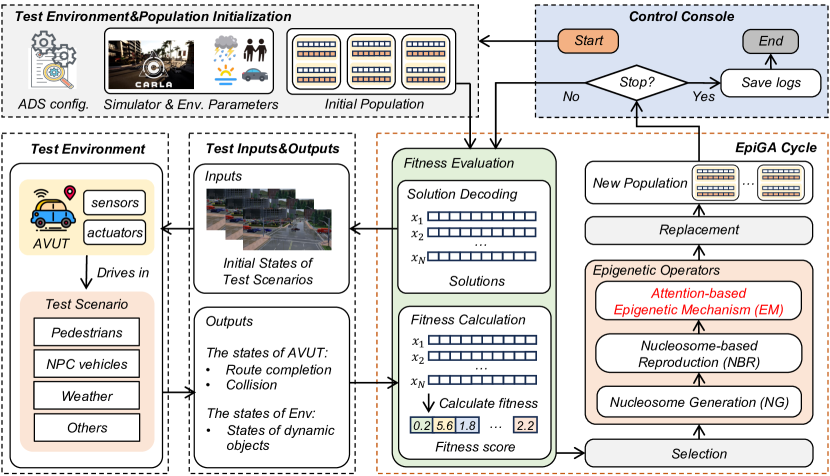
Figure 1: Overview of EpiTESTER. Control Console controls the start and end of the EpiTESTER workflow; Test Environment$\&$Population Initialization initializes the test environment and population for epiGA; Test Environment is a simulated environment where the AVUT drives in various test scenarios; Test inputs$\&$Outputs specify the inputs and outputs for the AV testing problem that EpiTESTER solves; EpiGA Cycle is the place where epiGA is employed, and the Epigenetic Mechanism (EM) has been extended based on the attention mechanism by EpiTESTER.

Figure 1 depicts the overall working mechanism of EpiTESTER. Control Console starts the workflow and evaluates the stopping criteria in each cycle. Each cycle starts with Test Environment$\&$Population Initialization. Specifically, the test environment is initialized, i.e., starting the simulator and loading the configurable environmental parameters, configuring the ADS, and deploying it to the AVUT. The initialization generates an initial population containing all encoded initial test solutions. Each encoded solution needs to be decoded into a test input (i.e., the initial state of the test scenario) during Solution Decoding before being fed into Test Environment. Test Environment then simulates test scenarios where the AVUT drives in. After that, a list of outputs, including states of the AVUT and the environment, is returned to Fitness Calculation for each solution’s fitness score. Then, EpiTESTER’s EpiGA Cycle starts, which is essentially the application of a sequence of genetic and epigenetic operators: the Selection operator, three Epigenetic Operators, and the Replacement operator. We apply GS as the Epigenetic Mechanism (EM), which controls the expression of each gene based on the attention mechanism. More details about the EpiGA Cycle will be introduced in Section 4.1, and the attention-based GS probability generation will be introduced in Section 4.2. Eventually, a new population is generated, and the workflow continues if the termination condition is not met; otherwise, the workflow terminates.

4.1 EpiGA-guided Scenario Generation

We employ epiGA [17] as our optimization algorithm. Since the optimization problem encoding is novel, we provide detailed discussions of each genetic and epigenetic operator in the subsequent subsections. Below, we first describe three genetic operators: initialization, selection, and replacement in Section 4.1.1, then present two epigenetic operators (i.e., nucleosome generation and nucleosome-based reproduction) in Section 4.1.2, and finally, we introduce the epigenetic mechanism that EpiTESTER applies, i.e., GS, in Section 4.1.3.

4.1.1 Population Initialization, Selection and Replacement

A population $P$ contains a set of $T$ individuals generated randomly. Once it is created, the EpiGA cycle begins. In contrast to the conventional behavior, where each individual encodes a solution to the problem being solved, in epiGA, each individual has $M$ cells. Each cell represents a distinct solution to the problem. As illustrated with the example shown in Figure 2(a), each cell of an individual has two vectors (i.e., $x$ and $n$). The length of each vector is equal to the number of configurable parameters (Section 3.2). The $x$ vector encodes the solution, whereas $n$ represents the nucleosome structure for the binary mask, which controls changes in each gene with a binary encoding during nucleosome-based reproduction. Concretely, the value in position $j$ of $n$ being 1 (i.e., $n_{j}=1$) means that the same position in the solution $x$ (i.e., $x_{j}$) is unchangeable (i.e., collapsed); if $n_{j}$ equals 0, it means that $x_{j}$ can be changed (i.e., uncollapsed).

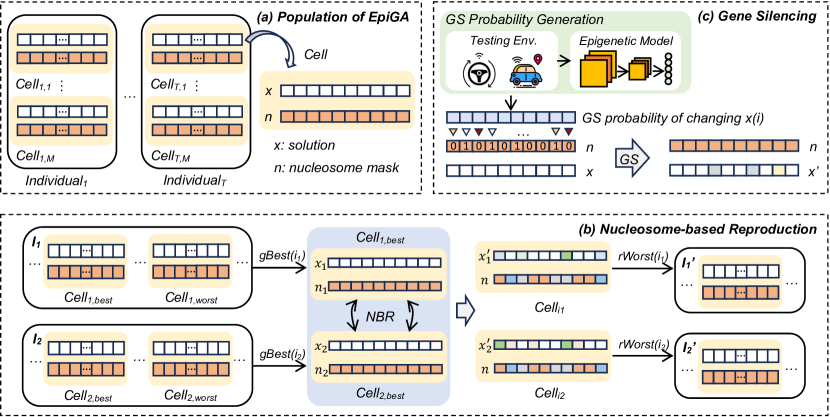
Figure 2: EpiTESTER’s Population Structure, Nucleosome-based Reproduction, and Gene Silencing. Sub-figure (a) illustrates that the population $P$ contains $T$ individuals each with $M$ cells. Each cell has two vectors: solution $x$ and nucleosome mask $n$; sub-figure (b) illustrates the nucleosome-based reproduction (NBR) process of reproducing new offspring by recombing solutions from parents with the guidance of nucleosome mask, among which functions $gBest()$ and $rWorst()$ obtain the best cell from an individual for NBR and replace the worst cell with new offspring, respectively; sub-figure (c) illustrates the epigenetic mechanism that EpiTESTER has extended and applied, i.e., gene silencing.

We use binary tournament selection [44] as the selection operator, commonly applied in GAs. This operator selects the fittest individuals from the current generation and passes them to subsequent operators.

As for the replacement operator, we employed the elitist replacement [45] to select and preserve the best individuals for the next generation.

4.1.2 Nucleosome Generation (NG) and Nucleosome-based Reproduction (NBR)

For population $P$, NG generates a new nucleosome vector ($n$) as a mask for each cell in each individual based on nucleosome probability $Pr_{n}$ and nucleosome radius $R$. In detail, for position $k$ of $n$ (i.e., $n_{k}$), if a randomized value $rand()$ is less than $Pr_{n}$, NG starts to collapse positions around $n_{k}$, i.e., setting their values as 1. Which positions to be collapsed around $n_{k}$ are determined by $R$: $max(\textit{k-R},0)$ to $min(\textit{k+R},len(n))$.

The NBR operator reproduces new offspring by recombining solutions from parents, guided by the nucleosome mask. As shown in Figure 2(b), NBR performs on two individuals (i.e., $I_{1}$ and $I_{2}$) from the current population $P$. First, according to fitness values, the best cells $c_{1}$ and $c_{2}$ are extracted from $I_{1}$ and $I_{2}$, respectively. Next, NBR is performed on $c_{1}$ and $c_{2}$ to produce new cells. As described in Algorithm 1, to generate new cells, NBR first calculates a new nucleosome mask $n$ as $n_{1}\textbf{OR}n_{2}$, where $n_{1}$ and $n_{2}$ are nucleosomes of $c_{1}$ and $c_{2}$. The logic is that for a position $j$, if one of $n_{1}(j)$ and $n_{2}(j)$ is collapsed (i.e., 1), then the corresponding position in $n$ will also be collapsed. Then, for those uncollapsed positions (i.e., 0), their corresponding values of $x_{1}$ and $x_{2}$ in those positions are swapped (Lines 6-12), and new solutions $x_{1}^{\prime}$ and $x_{2}^{\prime}$ are then produced. Eventually, two new cells $c_{1}$ and $c_{2}$ (Line 14) are created with the new nucleosome and solutions. The two new cells replace the two worst cells in $I_{1}$ and $I_{2}$; consequently, two new individuals are generated, i.e., $I_{1}^{\prime}$ and $I_{2}^{\prime}$.

Algorithm 1 Nucleosome-based Reproduction (NBR)

1:function NucleosomeBasedReproductionCell($c_{1}$, $c_{2}$)

2:    $x_{1}$, $x_{2}\leftarrow\textsc{GetSolution}(c_{1}),\textsc{GetSolution}(c_{2})$

3:    $n_{1}$, $n_{2}$ $\leftarrow$ $\textsc{getNucleosome}(c_{1})$, $\textsc{getNucleosome}(c_{2})$

4:    $n\leftarrow n_{1}\textbf{OR}n_{2}$

5:    for $j$ $\in$ ($1,\textsc{Len}(n))$ do

6:         if $n(j)$ then

7:             $x_{1}^{\prime}(j)\leftarrow x_{1}(j)$

8:             $x_{2}^{\prime}(j)\leftarrow x_{2}(j)$

9:         else

10:             $x_{1}^{\prime}(j)\leftarrow x_{2}(j)$

11:             $x_{2}^{\prime}(j)\leftarrow x_{1}(j)$

12:         end if

13:    end for

14:    $c_{1}^{\prime},c_{2}^{\prime}\leftarrow\textsc{Cell}(x1^{\prime},n),\textsc{Cell}(x2^{\prime},n)$

15:    return $c_{1}^{\prime},c_{2}^{\prime}$

16:end function

Algorithm 2 Gene Silencing (GS)

1:function GeneSilencingCell($c$, $Pr_{gs}$)

2:    $x$ $\leftarrow\textsc{GetSolution}(c)$

3:    $n_{1}$ $\leftarrow$ $\textsc{getNucleosome}(c)$

4:    for $j$ $\in$ ($1,\textsc{Len}(n))$ do

5:         if $n(j)\land rnd()<Pr_{e}$ then

6:             if $rnd()>Pr_{gs}(j)$ then

7:                 $\textsc{Express}(x(j))$

8:             end if

9:         end if

10:    end for

11:    return $c_{1}^{\prime},c_{2}^{\prime}$

12:end function

4.1.3 Epigenetic Mechanisms (EM)

In this paper, we extended the implementation of GS proposed by Stolfi et al. [17] for encoding the dynamic driving environment of the AVUT. GS regulates gene expression in a cell to prevent the expression of a certain gene through DNA methylation [30]. As illustrated in Figure 1(c), the core of EpiTESTER’s GS is GS Probability Generation (EG), which generates GS probabilities from the environment. GS probabilities ($Pr_{gs}$) is a vector of probabilities indicating the likelihood of changing each gene/position in solution $x$. As shown in Algorithm 2, the expression of each gene in $x$ is the effect of the nucleosome $n$, the epigenetic probability $Pr_{e}$, and GS probabilities $Pr_{gs}$. $Pr_{e}$ is a hyperparameter of epiGA, which controls whether GS takes effect. For example, only if position $k$ in $n$ is collapsed, $x(k)$’s value has a probability of $Pr_{gs}(k)$ to be changed.

Different from the original epiGA, which uses equal GS probabilities (i.e., 0.5) for all the positions, EpiTESTER is embedded with a machine learning model, namely Epigenetic Model, to generate GS probabilities from the environment. We build the model based on a multi-modal fusion transformer [46] and attention mechanism. The model receives observations from the environment and generates GS probabilities accordingly. The details of EG will be introduced in Section 4.2.

4.2 Attention-based GS Probability Generation

As discussed in Section 4.1.3, EpiTESTER adopts GS as its epigenetic mechanism, where a machine learning model called Epigenetic Model is employed to generate GS probabilities. Concretely, as Figure 3 shows, Epigenetic Model receives states/observations (i.e., RGB image and LiDAR bird’s-eye view (BEV)) from the test environment and adaptively generates GS probability for each configurable environment parameter. Adaptively doing this, rather than uniformly and statically assigning an equal probability to all parameters, stems from the dynamic and continuously evolving nature of the operating environment of AVUT, which consequently exerts distinct effects on the behavior of the AVUT [47].

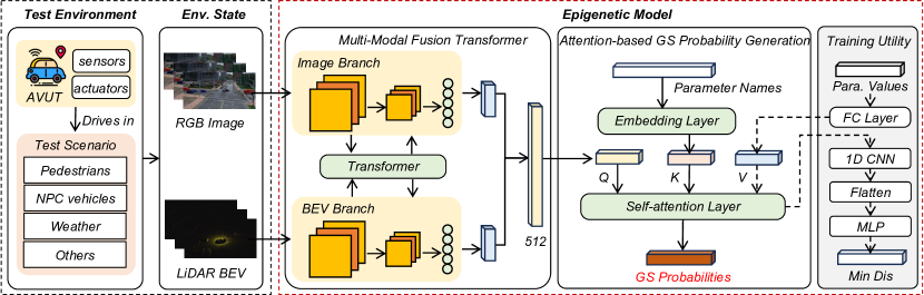
Figure 3: Overview of GS Probability Generation.

Considering that the AVUT senses the test environment from multiple data modalities such as images and LiDAR point clouds, we adopt a Multi-Modal Fusion Transformer [46] (Section 4.2.1) to fuse image and LiDAR point clouds as encodings of environmental states. The transformer extracts high-level features from environmental states, and then the extracted features are inputted into Attention-Based GS Probability Generation (Section 4.2.2) to calculate the GS probabilities. Besides, to train the model, we employ another module named Training Utility (Section 4.2.3).

4.2.1 Multi-Modal Fusion Transformer (MMFT)

To design MMFT, we take inspiration from the transformer-based sensor fusion architecture proposed in Transfuser [46]. Transfuser is a novel model architecture for end-to-end autonomous driving, and it is ranked fourth place in autonomous driving on CARLA leaderboard, demonstrating its state-of-the-art sensor fusion ability. MMFT takes RGB and BEV images as its input and outputs a 48-dimensional feature vector representing the state encodings of the environment. Specifically, we follow the same input representations that use three camera images (front, left, right) and compose them into a single three-channel RGB image with $960\times 160$ pixels. The BEV image is represented as a three-channel pseudo-image of size $336\times 150$ pixels. The Image Branch and BEV Branch are designed as two regular networks (RegNet) [48] with the same network structures employed by Transfuser. As for Transformer, different from Transfuser that employs four transformer modules, we use one module because we experimented with various settings and found that one module has already achieved comparable prediction results with less training time.

4.2.2 Attention-Based GS Probability Generation (AGPG)

As shown in Figure 3, AGPG contains two layers: Embedding Layer and Self-attention Layer.

Embedding Layer (Emb) maps discrete input tokens such as words to continuous embedding vectors in a high-dimensional space, where the vectors are a representation of the semantics of tokens, efficiently encoding semantic information that might be relevant to the task at hand [49]. As Figure 3 shows, it accepts a 10-dimensional vector (i.e., Para. Names) of strings encoding the names of the configurable environment parameters as its input and outputs word embeddings as $\textbf{K}\in\mathbb{R}^{N_{k}\times D_{k}}$, where $N_{k}$ is the number of parameter names and each name is represented as a 1-dimensional feature vector of size $D_{k}$.

Self-attention Layer (Attn) calculates the attention weights between the state encoding and the word embeddings as the GS probabilities. Concretely, we exploit the self-attention mechanism to map a set of queries ($\textbf{Q}\in\mathbb{R}^{N_{q}\times D_{q}}$), keys ($\textbf{K}\in\mathbb{R}^{N_{k}\times D_{k}}$), and values ($\textbf{V}\in\mathbb{R}^{N_{v}\times D_{v}}$) to outputs, where Q is calculated as the state encoding by MMFT, and K are the word embeddings of the parameter names, and V is calculated by the FC Layer employed in Training Utility:

$$\textbf{Q}=\textsc{Mmft}(RGB,BEV),\textbf{K}=\textsc{Emb}(\textit{PN}),\textbf{V}=FC(\textit{PV}).$$ (4)

We then calculate the attention weights A using the scaled dot products between Q and K:

$$\textbf{A}=sigmoid(\dfrac{Q\cdot K^{T}}{\sqrt{d_{k}}}).$$ (5)

As explained in Section 2.2, we employ the sigmoid as the activation function, and the scaling factor $1/\sqrt{d_{k}}$ is introduced to counteract the effect of having the dot products grow large in magnitude.

Notice that in our problem, $\textbf{Q}\in\mathbb{R}^{1\times 48}$, $\textbf{K}\in\mathbb{R}^{10\times 48}$, and $\textbf{V}\in\mathbb{R}^{1\times 10}$, therefore $\textbf{A}\in\mathbb{R}^{1\times 10}$, which is a vector of 10 values. For a value $\textbf{A}_{i}$ in position $i$, it can be denoted as the dot product between the state encodings and the word embedding of the $i$ parameter name: $\textbf{Q}\cdot K_{i}^{T}$ indicating $ith$ parameter’s contribution to the output. The attention weights are continuously optimized as the training proceeds, and after the model has been trained, we use the attention weights as probabilities of changing/silencing each gene in a solution, i.e., GS probabilities.

In addition, the output of the attention layer is denoted as the concatenation of Q, the dot products between A and V ($\textbf{A}\cdot\textbf{V}$), and V:

$$\textbf{O}_{\textbf{attn}}=concatenate(A\cdot V,Q,V)=A\cdot V+Q+V,$$ (6)

where $\textbf{A}\cdot\textbf{V}$ is computed as a weighted sum of the values of V, whereas Q and V are directly connected to the output, referred to as shortcut connections. Shortcut connection is a commonly applied technique in Residual Networks [50], which has been shown effective in preventing vanishing/exploding gradients. For training the network, $\textbf{O}_{\textbf{attn}}$ is further passed into Training Utility.

4.2.3 Training Utility

This module trains Epigenetic Model. Once the model is well-trained, it is used for generating GS probabilities. The training utility’s architecture is shown in Figure 3. Specifically, it takes a 10-dimensional vector representing the values of the configurable environmental parameters (Para. Values) as its input and passes it to the FC Layer with 10 neurons. The output of the FC Layer is passed to the Self-attention Layer in AGPG (Section 4.2.2) to get $\textbf{O}_{\textbf{attn}}$. $\textbf{O}_{\textbf{attn}}$ is a 106-dimensional vector, and we pass it to a 1-dimensional convolutional (Conv1D) network (i.e., 1D CNN). The 1D CNN has four Conv1D layers with the kernel sizes being 16, 32, 64, and 32, respectively. The output of 1D CNN is then passed to the Flatten Layer and will be flattened into a 3136-dimensional vector. Finally, the output is passed to the multi-layer perception (MLP), which predicts the fitness value (i.e., the minimum distance as discussed in 3.2). The MLP contains four fully connected layers with the neuron numbers 512, 256, 128, and 1, respectively. We calculate smooth L1 loss between the predicted fitness value $f$ and ground truth fitness value:

$$\mathcal{L}=\begin{cases}\dfrac{1}{n}\sum_{i=1}^{n}\dfrac{1}{2}({f_{gt}}_{i}-f_{i})^{2},|{f_{gt}}_{i}-f_{i}|<1\\ \\ \dfrac{1}{n}\sum_{i=1}^{n}(|{f_{gt}}_{i}-f_{i}|-0.5),\text{otherwise}\end{cases}$$ (7)

5 Experiment Design

5.1 Research Questions

We evaluate EpiTESTER by answering the following three research questions (RQs).

• RQ1: How effective is EpiTESTER compared to the two baseline methods?

• RQ2: How efficiently does EpiTESTER perform compared to the baseline methods?

• RQ3: How does gene silencing affect the gene expression (i.e., selection of parameters) in EpiTESTER and $\textit{EpiTESTER}_{eq}$?

5.2 Subject System and Simulator

To evaluate EpiTESTER, we employed Interfuser [23] as the system under test, which is an end-to-end ADS ranked the first place on the CARLA leaderboard. Interfuser has been evaluated in various driving situations from the CARLA public leaderboard, the Town05 benchmark [51], and the CARLA 42 Routes benchmark [52], demonstrating its outstanding performance in comprehensive scene understanding and adversarial event detection.

For the simulator, we adopted CARLA [24], an open-source and widely-applied autonomous driving simulator, to simulate the AVUT and its driving environment. CARLA provides an extensive list of digital assets, including vehicles, pedestrians, sensors, and high-definition maps, for supporting the development, training, and validation of AVs. In our experiments, we used CARLA-0.9.10.1 and its default Interfuser settings. The AVUT controlled by Interfuser is the Tesla Model 3, which has been used in various autonomous driving research contexts [53].

5.3 Baselines

As Arcuri and Briand suggested [54], random strategies (RS) are usually used for sanity checks; therefore, to check if our problem is complex, we performed a pilot study to compare EpiTESTER with RS. Results show that EpiTESTER is significantly better than RS in collision scenario generation. Hence, our formal experiment excluded RS as a baseline. The detailed results of the pilot study are provided in our online repository (see Section 6.5).

To answer RQs, we employed two baselines, including a classical GA (i.e., GA) [55] without any epigenetic mechanism implemented, and a modified EpiTESTER, i.e., $\textit{EpiTESTER}_{eq}$, which sets equal GS probabilities for each gene, i.e., environmental parameters. GA is a widely applied, single-objective metaheuristic algorithm that uses biologically inspired genetic operators such as mutation, crossover, and selection to solve search problems. For our experiments, we implemented GA using jMetalPy [56], a well-known framework for single/multi-objective optimization. $\textit{EpiTESTER}_{eq}$ uses equal GS probabilities for each gene, i.e., 0.5, the default setting employed by epiGA [17]. This means that each gene has the same chance to be silenced or expressed, which further implies that each gene is treated equally, and for each gene, the probability of being activated and silenced is equal to 0.5.

5.4 Parameter Settings

Since the parameters of EpiTESTER, $\textit{EpiTESTER}_{eq}$, and GA greatly impact the algorithm’s performance, finding appropriate parameter settings for genetic and epigenetic algorithms is crucial to obtaining optimal results and fair comparisons. Therefore, to determine the parameters for GA and epiGA employed by EpiTESTER and $\textit{EpiTESTER}_{eq}$, we experimented with different combinations of the key parameters. As a result, we set the population size as 20 and the number of cells in each individual of EpiTESTER and $\textit{EpiTESTER}_{eq}$ as 1. Besides, the termination criterion is the maximum number of evaluations, i.e., 1000. In addition, we set the nucleosome probability $Pr_{n}$ as 0.2, the nucleosome radius $R$ as 1, and the epigenetic probability $Pr_{e}$ as 0.01 (Section 4.1.2).

As for hyperparameter settings for training the epigenetic model of EpiTESTER, we set the batch size and number of epochs to 64 and 10000 based on the results of our pilot study. For the other hyperparameters, we followed the same settings as the model from Transfuser. To train the epigenetic model, we first built a dataset by running a random strategy. As a result, we obtained a dataset containing about 25k samples, each labeled with a fitness value, i.e., minimum distance. Since the epigenetic model aims to calculate attention weights to represent the GS probability for each gene that can potentially contribute to collisions or safety violations of the AVUT, samples with higher chances (i.e., smaller minimum distances) of causing safety violations are more important. Therefore, we filter out records in the dataset with a minimum distance greater than 5 meters. In the end, we obtained a dataset of around 5000 samples. We follow the 80%/20% training/test split ratio to split the dataset into a training and a test dataset, as suggested by Rácz et al. [57]. The model was trained on the training dataset and converged with a loss value 0.019. We evaluated the trained model on the test dataset and obtained a mean square error (i.e., MSE) of 0.027 and a mean absolute error (i.e., MAE) of 0.16, indicating the prediction error for the minimum distance is about 0.16m, which is acceptable since the minimum distance ranges from 0 to 5m. The pilot study results, the epigenetic model parameter settings, and training details are available in our online repository (see Section 6.5).

5.5 Test Environment Initialization and Execution

EpiTESTER identifies critical scenarios by configuring an initial test environment, i.e., introducing a NPC vehicle and a pedestrian, and manipulating the weather as discussed in Section 3.2. In our design, an initial test environment specifies the map, the AVUT’s driving route, and existing traffic users such as vehicles. The driving route specifies that the AVUT should drive from a starting point to a destination without collisions. Notice that in the initial environment, the AVUT can navigate safely to the destination if no additional environmental scenario element (e.g., the NPC vehicle and weather) is introduced, and EpiTESTER’s goal is to introduce new environmental scenario elements that can cause collisions or other safety violations. In our experiment, we select four initial environments, i.e., $Env_{1}$, $Env_{2}$, $Env_{3}$, and $Env_{4}$, as described in Figure 4.

(a) $Env_{1}$

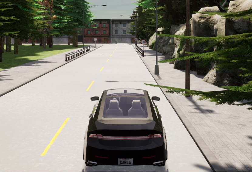
(b) $Env_{2}$

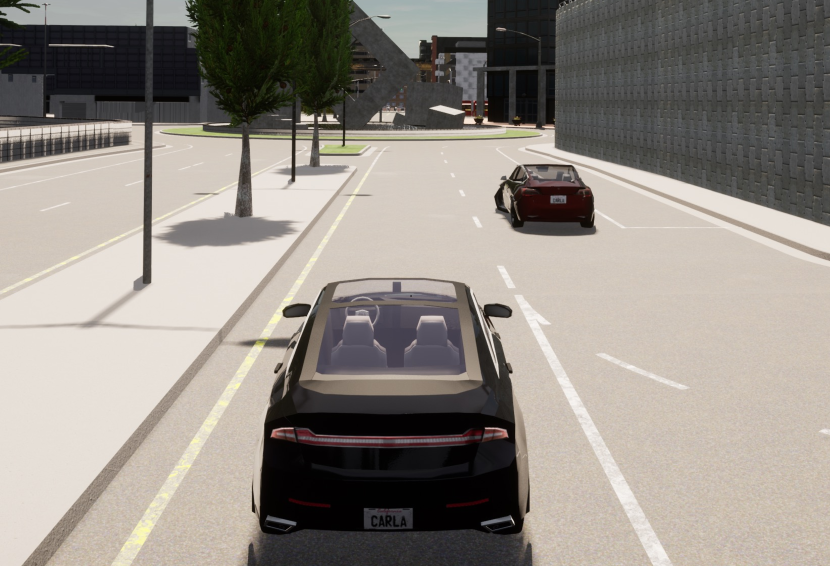
(c) $Env_{3}$

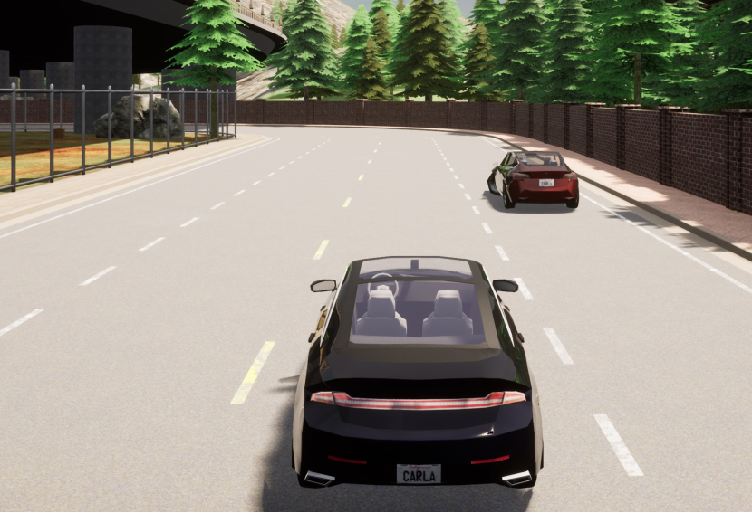
(d) $Env_{4}$

Figure 4: Initial Driving Environments of the AVUT. Sub-figure 4(a) depicts $Env_{1}$ where the AVUT is driving along a one-way road with four lanes of the Town04 map. The AVUT is expected to change lanes twice from the leftmost lane to the rightmost and then maintain the lane until arriving at its destination; sub-figure 4(b) depicts $Env_{2}$ where the AVUT is driving along a dual-way road with two opposite lanes of the Town2 map. The AVUT is expected to maintain its current lane until arriving at its destination; sub-figure 4(c) depicts $Env_{3}$ where the AVUT is driving along a dual-way road with two opposite lanes and then entering into a one-way road with two lanes of the Town03 map. Meanwhile, a red sedan is trying to switch from its current lane to the left lane; sub-figure 4(d) depicts $Env_{4}$ where the AVUT is driving along a dual-way four-lane road with two lanes in each direction of the Twon05 map. Meanwhile, a red sedan is trying to switch from its current lane to the left lane.

To account for the randomness caused by the AVUT and the simulator we used, we executed EpiTESTER, GA, and $\textit{EpiTESTER}_{eq}$ 10 runs on each initial environment. After each run, we obtained a solution (i.e., test input), and we further executed it 30 times to deal with the AVUT and simulator randomness. Finally, we obtained results of 3600 executions (3 methods $\times$ 4 initial environments $\times$ 10 runs $\times$ 30 executions).

All experiments were executed on one server node with an Intel Xeon Platinum 8186, 8$\times$NVIDIA A100 GPU.

5.6 Evaluation Metrics and Statistical Tests

To evaluate the performance of EpiTESTER and the baselines, we adopt five metrics commonly used in AV development and testing [46, 58]:

1. Minimum Distance (MD) measures the minimum distance between the AVUT and its surrounding objects. A lower MD value indicates a higher chance of safety violations. For the $kth$ execution of solution $s$, MD is calculated as: $MD_{s}^{k}=\mathcal{F}_{s}(AVUT,obj_{s})$, where $F_{s}$ is the fitness function (Section 3.2).

2. Collision (CO) indicates whether the AVUT collided with any object. For the $kth$ execution of solution $s$, $CO_{s}^{k}\in\{0,1\}$, where 0 and 1 denote no collision occurred and a collision happened, respectively;

3. Route Completion (RC) defines the percentage of route distance completed by the AVUT. $RC_{s}^{k}$ denotes the route completion of the $kth$ execution of solution $s$. A lower $RC_{s}^{k}$ indicates $s$ caused the AVUT to complete less route distance, e.g., caused by collisions or traffic jams.

4. Infraction Score (IS) calculates geometric series of infraction penalty coefficients, with lower IS values indicating more serious infractions occurred. IS for the $kth$ execution of solution $s$ is calculated as:

   $$IS_{s}^{k}=\prod_{j}^{ped,npc,sta}(p^{j})^{(\#infractions^{j})}$$ (8)

   where $p_{j}$ is the penalty coefficient of infraction $j$, and $\#infractions^{j}$ denotes the number of $infractions^{j}$ occurred. We consider three types of infraction, i.e., collision with a pedestrian ($ped$), collision with a NPC vehicle ($npc$), and collision with a static object ($sta$). According to the CARLA leaderboard, the penalty coefficient for each infraction is 0.50, 0.60, and 0.65, respectively.

5. Driving Score (DS), as a comprehensive metric, calculates the weighted route completion (RC) with infraction score (IS). A lower DS value indicates poorer AVUT’s overall driving performance. DS for the $kth$ execution of solution $s$ is calculated as the product of RC and IS: $DS_{s}^{k}=RC_{s}^{k}\cdot IS_{s}^{k}$.

Statistical Test. Based on the guidelines [54], we first perform the Mann-Whitney U test with a significance level of 0.05 to study the statistical significance of two methods and then use the Vargha and Delaney effect size to calculate $\hat{A}_{12}$. The effect size $\hat{A}_{12}$ indicates the chance of method A yielding higher values of a metric $\chi$ than method B. If $\hat{A}_{12}$ is greater than 0.5, then A has a higher chance to obtain higher values of $\chi$ than B, and vice versa.

To study the correlation between MD and other metrics (i.e., CO, RC, IS, and DS), we perform the Spearman’s rank correlation ($\rho$) test, a non-parametric test that measures the monotonic relationship between two ranked variables. $\rho\in(0,1]$ indicates a positive correlation and $\rho\in[-1,0)$ shows a negative correlation. A value of 1.0 (-1.0) indicates a perfect positive (negative) correlation, and 0 means no correlation. The significance of a correlation is indicated with a p-value less than 0.05. Based on the guidelines by Mukaka [59], we further divide $\rho$ into five levels to interpret the magnitude of a correlation: negligible ($\rho$ $\in$ (-0.300, 0.300)), low ($\rho$ $\in$ [0.300, 0.500) or (-0.500, -0.300]), moderate ($\rho$ $\in$ [0.50, 0.700) or (-0.700, 0.500]), high ($\rho$ $\in$ [0.700, 0.900) or (-0.900, -0.700]), and very high ($\rho$ $\in$ [0.900, 1.000] or [-1.000, -0.900]).

6 Experiment Results and Analyses

6.1 Results for RQ1 - Effectiveness

To answer RQ1, we compared the effectiveness of EpiTESTER with $\textit{EpiTESTER}_{eq}$ and GA regarding all metrics under the four initial driving environments (i.e., $Env_{1}$, $Env_{2}$, $Env_{3}$, and $Env_{4}$) and across them (i.e., $Env_{1-4}$).

Statistical Differences. Results of the Mann and Whitney U test and Vargha and Delaney effect size are reported in Table I.

TABLE I: Results of pair-wise comparisons of EpiTESTER with the baseline methods (i.e., GA and $\textit{EpiTESTER}_{eq}$) using the Vargha and Delaney statistics and the Mann–Whitney U test – RQ1. ”$\downarrow$ / $\uparrow$” denotes that a smaller/larger metric value indicates a better performance of a method. A bold $\hat{A}_{12}$ with a p-value $<$ 0.05 implies that EpiTESTER is significantly better than GA/$\textit{EpiTESTER}_{eq}$. A $\hat{A}_{12}$ with symbol ”×” indicates that EpiTESTER significantly underperformed GA/$\textit{EpiTESTER}_{eq}$.

Initial Env.	EpiTESTER vs. baselines	$MD\downarrow$		$CO\uparrow$		$RC\downarrow$		$IS\downarrow$		$DS\downarrow$
		$\hat{A}_{12}$	p-value	$\hat{A}_{12}$	p-value	$\hat{A}_{12}$	p-value	$\hat{A}_{12}$	p-value	$\hat{A}_{12}$	p-value
$Env_{1}$	GA	0.347	$<$0.05	0.658	$<$0.05	0.551×	$<$0.05	0.388	$<$0.05	0.522	0.337
	$\textit{EpiTESTER}_{eq}$	0.468	$<$0.05	0.535	$<$0.05	0.449	$<$0.05	0.465	$<$0.05	0.445	$<$0.05
$Env_{2}$	GA	0.302	$<$0.05	0.698	$<$0.05	0.564×	$<$0.05	0.302	$<$0.05	0.481	0.413
	$\textit{EpiTESTER}_{eq}$	0.418	$<$0.05	0.573	$<$0.05	0.578×	$<$0.05	0.427	$<$0.05	0.540	0.089
$Env_{3}$	GA	0.387	$<$0.05	0.613	$<$0.05	0.608×	$<$0.05	0.454	$<$0.05	0.458	0.068
	$\textit{EpiTESTER}_{eq}$	0.502	0.699	0.498	0.705	0.455	$<$0.05	0.502	0.705	0.459	0.065
$Env_{4}$	GA	0.339	$<$0.05	0.662	$<$0.05	0.268	$<$0.05	0.477	0.231	0.240	$<$0.05
	$\textit{EpiTESTER}_{eq}$	0.497	0.467	0.503	0.478	0.291	$<$0.05	0.546×	$<$0.05	0.292	$<$0.05
$Env_{1-4}$	GA	0.481	$<$0.05	0.519	$<$0.05	0.461	$<$0.05	0.479	$<$0.05	0.459	$<$0.05
	$\textit{EpiTESTER}_{eq}$	0.351	$<$0.05	0.650	$<$0.05	0.480	0.091	0.391	$<$0.05	0.433	$<$0.05

Regarding MD, EpiTESTER significantly outperformed GA for all four initial environments, i.e., $\hat{A}_{12}<0.5$ and $\textit{p-value}<0.05$. EpiTESTER also significantly outperformed $\textit{EpiTESTER}_{eq}$ in $Env_{1}$ and $Env_{2}$ and achieved comparable performance with $\textit{EpiTESTER}_{eq}$ for $Env_{3}$ and $Env_{4}$. Similarly, for CO, EpiTESTER significantly outperformed GA for all initial environments regarding leading the AVUT to collideand significantly outperformed $\textit{EpiTESTER}_{eq}$ in $Env_{1}$ and $Env_{2}$ and achieved comparable performance with $\textit{EpiTESTER}_{eq}$ in $Env_{3}$ and $Env_{4}$.

Regarding RC, we can observe that EpiTESTER performed significantly better (i.e., lower route completion) than GA in $Env_{4}$, while it significantly underperformed GA in $Env_{1}$, $Env_{2}$, and $Env_{3}$. EpiTESTER significantly outperformed $\textit{EpiTESTER}_{eq}$ in $Env_{1}$, $Env_{3}$, and $Env_{4}$ and underperformed in $Env_{2}$. These observations show that, in most cases, EpiTESTER can cause the AVUT to collide earlier and, therefore, complete less route distance than $\textit{EpiTESTER}_{eq}$ and GA. After replaying generated scenarios, we observed cases that EpiTESTER led the AVUT to collide, but it continued to drive forward. Hence, RC further increases. However, GA generated scenarios can cause the AVUT to get stuck in traffic jams or blocked by its front obstacles, achieving better performance in RC. We also observed a similar situation in $Env_{2}$ for $\textit{EpiTESTER}_{eq}$. Therefore, in EpiTESTER, low RC values are mainly caused by collisions, not unrealistic traffic jams, etc.

Regarding IS, EpiTESTER outperformed GA in all initial environments, and for $Env_{1}$, $Env_{2}$, and $Env_{3}$ the differences are significant, i.e., p-value$<$0.05. EpiTESTER performed significantly better than $\textit{EpiTESTER}_{eq}$ in $Env_{1}$ and $Env_{2}$, while there is no significant difference in $Env_{3}$ can be observed. However, in $Env_{4}$, EpiTESTER significantly underperformed $\textit{EpiTESTER}_{eq}$. Recall that IS calculates the geometric series of penalty coefficients by considering three types of collisions: with dynamic objects (pedestrian and NPC vehicle) and with static objects. Each type is associated with a penalty coefficient indicating the collision’s severity, i.e., the smaller the coefficient, the more severe the collision. A higher penalty coefficient leads to a higher IS, which is computed by multiplying a penalty coefficient for every collision. Therefore, the result in $Env_{4}$ indicates that $\textit{EpiTESTER}_{eq}$ caused more collisions with lower penalty coefficients than EpiTESTER. To know why, we further analyzed scenarios that led to collisions and found that $\textit{EpiTESTER}_{eq}$ caused more collisions with pedestrians whose penalty coefficient is 0.5, while most collisions caused by EpiTESTER are with NPC vehicles whose penalty coefficient is 0.6. In CARLA leaderboard, collisions with pedestrians are considered more severe than those with NPC vehicles, so collisions with pedestrians have a lower penalty coefficient than those with NPC vehicles. However, there is evidence that collisions with trucks can cause more severe injuries to passengers than collisions with pedestrians [60].

Regarding DS, EpiTESTER achieved comparable performance with GA in $Env_{1}$, $Env_{2}$, and $Env_{3}$ and significantly outperformed GA in $Env_{4}$. EpiTESTER significantly outperformed $\textit{EpiTESTER}_{eq}$ in $Env_{1}$ and $Env_{4}$ and has no significant difference observed in $Env_{2}$ and $Env_{3}$. As a performance metric calculated by weighting RC and IS, the results for DS show that the AVUT performed similarly or significantly worse in scenarios generated by EpiTESTER than in those generated by GA and $\textit{EpiTESTER}_{eq}$.

Besides, when looking at the results by combining all four initial environments, i.e., row $Env_{1-4}$ in Table I, we can observe that, overall, EpiTESTER outperformed GA and $\textit{EpiTESTER}_{eq}$ in terms of all metrics, and the results of EpiTESTER are all significantly better except for the comparison with $\textit{EpiTESTER}_{eq}$ regarding RC.

Correlation Analysis among the Five Metrics. Considering that MD is the objective that EpiTESTER directly optimizes, we performed the Spearman’s rank correlation ($\rho$) test to study the correlation between MD and the other metrics and report the results in Table II. As the table shows, there is a high/very high and significant negative correlation between MD and CO for all three methods in all four environments, i.e., all $\rho$ values are near -1.0, and a high/very high and significant positive correlation between MD and IS for almost all cases (except for GA in $Env_{4}$). This is reasonable as the lower the distance between the AVUT and other objects, the higher the chance of more collisions and lower infraction scores. We can also observe negligible correlations between MD and RC/DS.

Distributions. We also present the descriptive statistics of results achieved by each method in Figure 5. Regarding MD, across all initial environments, EpiTESTER and $\textit{EpiTESTER}_{eq}$ achieved similar distributions of lower variability than those from GA. Similar patterns on the variability of the CO and IS distributions achieved by EpiTESTER and $\textit{EpiTESTER}_{eq}$ can be observed. This indicates that GS employed in both EpiTESTER and $\textit{EpiTESTER}_{eq}$ is reliable in directly reducing MD (as it is the optimization objective) and indirectly increasing CO and reducing IS. For RC and DS, the distributions obtained by EpiTESTER and $\textit{EpiTESTER}_{eq}$ also have lower variability than those from GA. When looking across the different metrics, the results on RC and DS are less reliable than those on MD, CO, and IS. This observation further confirms the results of the correlation analyses.

TABLE II: Results of correlations between MD and CO, RC, IS, and DS using the Spearman’s rank correlation ($\rho$) test. A $\rho$ value decorated by a $\color[rgb]{0,0,1}\blacktriangle$ indicates that MD has a high/very high and significant positive/negative correlation with another metric, i.e., $\rho$ $\in$ [0.700, 1.000] or [-1.000, -0.700] and $\textit{p-value}<0.05$. A $\rho$ value decorated with a $\bullet$ indicates insignificant correlation between MD and another metric.

Initial Env.	Method	MD$\downarrow$ vs.
		CO$\uparrow$	RC$\downarrow$	IS$\downarrow$	DS$\downarrow$
$Env_{1}$	EpiTESTER	-0.999 $\color[rgb]{0,0,1}\blacktriangle$	-0.129	0.999 $\color[rgb]{0,0,1}\blacktriangle$	0.051 $\bullet$
	GA	-0.963 $\color[rgb]{0,0,1}\blacktriangle$	-0.574	0.904 $\color[rgb]{0,0,1}\blacktriangle$	-0.484
	$\textit{EpiTESTER}_{eq}$	-0.996 $\color[rgb]{0,0,1}\blacktriangle$	0.282	0.996 $\color[rgb]{0,0,1}\blacktriangle$	0.424
$Env_{2}$	EpiTESTER	-0.983 $\color[rgb]{0,0,1}\blacktriangle$	-0.698	0.983 $\color[rgb]{0,0,1}\blacktriangle$	-0.134
	GA	-0.829 $\color[rgb]{0,0,1}\blacktriangle$	-0.523	0.829 $\color[rgb]{0,0,1}\blacktriangle$	-0.202
	$\textit{EpiTESTER}_{eq}$	-0.953 $\color[rgb]{0,0,1}\blacktriangle$	-0.764 $\color[rgb]{0,0,1}\blacktriangle$	0.953 $\color[rgb]{0,0,1}\blacktriangle$	-0.312
$Env_{3}$	EpiTESTER	-1.000 $\color[rgb]{0,0,1}\blacktriangle$	-0.189	1.000 $\color[rgb]{0,0,1}\blacktriangle$	0.209
	GA	-0.988 $\color[rgb]{0,0,1}\blacktriangle$	-0.572	0.848 $\color[rgb]{0,0,1}\blacktriangle$	0.546
	$\textit{EpiTESTER}_{eq}$	-1.000 $\color[rgb]{0,0,1}\blacktriangle$	-0.180	1.000 $\color[rgb]{0,0,1}\blacktriangle$	0.186
$Env_{4}$	EpiTESTER	-0.999 $\color[rgb]{0,0,1}\blacktriangle$	0.138	0.999 $\color[rgb]{0,0,1}\blacktriangle$	0.392
	GA	-0.973 $\color[rgb]{0,0,1}\blacktriangle$	-0.392	0.845 $\color[rgb]{0,0,1}\blacktriangle$	-0.262
	$\textit{EpiTESTER}_{eq}$	-1.000 $\color[rgb]{0,0,1}\blacktriangle$	-0.136	0.398	0.033 $\bullet$
$Env_{1-4}$	EpiTESTER	-0.998 $\color[rgb]{0,0,1}\blacktriangle$	-0.209	0.673	0.118
	GA	-0.957 $\color[rgb]{0,0,1}\blacktriangle$	-0.442	0.874 $\color[rgb]{0,0,1}\blacktriangle$	-0.107
	$\textit{EpiTESTER}_{eq}$	-0.996 $\color[rgb]{0,0,1}\blacktriangle$	-0.304	0.743 $\color[rgb]{0,0,1}\blacktriangle$	0.021 $\bullet$

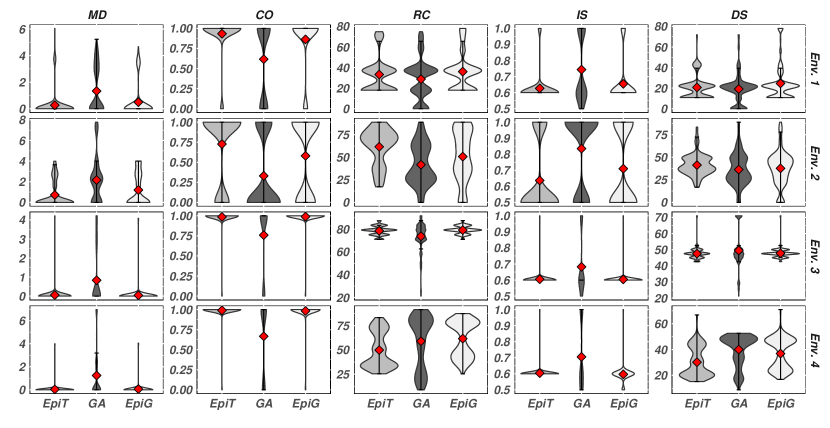
Figure 5: Descriptive statistics of all the metrics achieved by EpiTESTER, GA, and $\textit{EpiTESTER}_{eq}$– RQ1. EpiT is EpiTESTER and EpiG is $\textit{EpiTESTER}_{eq}$. $\color[rgb]{1,0,0}\mdblkdiamond$ denotes the mean value of each sample.

Conclusion for RQ1: Compared to $\textit{EpiTESTER}_{eq}$ and GA, EpiTESTER achieved the overall best performance regarding the selected metrics, and the differences are mostly significant. This indicates that EpiTESTER is more effective in generating critical scenarios that lead to shorter distances to other objects, more collision occurrences, and poorer driving performance of the AVUT, e.g., lower driving score.

6.2 Results for RQ2 - Efficiency

Recall that we set the population size as 20 and the number of generations as 50; therefore, the number of evaluations is 1000 for each method. We ran each method 10 times to account for the randomness. Therefore, for each run $r$ ($r$=1…10) of each method, we obtained 50 generations, and each has 20 solutions. We then calculate the average and the best fitness values (i.e., MD) for each generation of 20 solutions as $fitness_{avg}$ and $fitness_{best}$. Figure 6 presents how $fitness_{avg}$ and $fitness_{best}$ of the 10 runs vary in each generation of EpiTESTER, GA, and $\textit{EpiTESTER}_{eq}$ in each initial environment. Concretely, we report the mean values of $fitness_{avg}$ and $fitness_{best}$ of each generation with 95% confidence intervals.

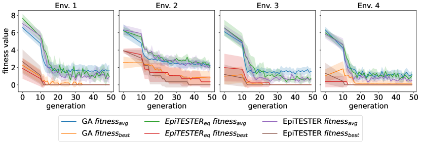
Figure 6: Average and best fitness values (i.e., $fitness_{avg}$ and $fitness_{best}$) achieved by EpiTESTER, GA, and $\textit{EpiTESTER}_{eq}$ with 95% confidence intervals in each generation – RQ2.

As shown in Figure 6, GA converged to higher $fitness_{avg}$ values than EpiTESTER and $\textit{EpiTESTER}_{eq}$ in all initial environments except for $Env_{2}$ where all three methods converged to a comparable $fitness_{avg}$. Besides, EpiTESTER and $\textit{EpiTESTER}_{eq}$ converged to a similar $fitness_{avg}$ in all initial environments, and in $Env_{4}$, EpiTESTER consistently performed better than $\textit{EpiTESTER}_{eq}$ throughout the 50 generations. When looking at the evolution along the generations, compared to $\textit{EpiTESTER}_{eq}$, EpiTESTER achieved faster convergence speeds in $Env_{1}$, $Env_{3}$, and $Env_{4}$, and a comparable convergence speed with $\textit{EpiTESTER}_{eq}$ in $Env_{2}$. This indicates that EpiTESTER is more efficient at minimizing the distance between the AVUT and other objects than $\textit{EpiTESTER}_{eq}$. GA quickly converged in the first 10 to 20 generations and then gradually slowed down. When comparing the variability of $fitness_{avg}$ achieved by the methods, we do not notice many differences, implying that they have comparable reliability.

As for $fitness_{best}$ in each generation of the three methods, we can see from Figure 6 that for all 10 runs, EpiTESTER can always find 0 as $fitness_{best}$ in all initial environments when converged, while GA and $\textit{EpiTESTER}_{eq}$ only find 0 as $fitness_{best}$ in $Env_{1}$ and $Env_{3}$ for all 10 runs. Besides, when looking at the number of generations needed to detect a collision (i.e., $fitness_{best}$=0), it is evident that EpiTESTER used fewer generations than GA and $\textit{EpiTESTER}_{eq}$, in all four environments, meaning that EpiTESTER is more efficient at detecting collisions. One can also notice that the variances of $fitness_{best}$ achieved by the three methods are all large initially and then smaller over generations. As for EpiTESTER, we can always observe no variability in terms of $fitness_{best}$ when it converged for all initial environments, while we can observe two such cases for GA (i.e., $Env_{1}$ and $Env_{3}$), and three such cases for $\textit{EpiTESTER}_{eq}$ (i.e., $Env_{1}$, $Env_{3}$, and $Env_{4}$).

Conclusion for RQ2: Compared to $\textit{EpiTESTER}_{eq}$ and GA, EpiTESTER achieved a faster convergence speed and used fewer generations to detect collisions. This shows that compared to the baseline methods, the EpiTESTER is not only more efficient at converging to shorter distances between AVUT and other objects but also more efficient at collision detection.

6.3 Results for RQ3 - Gene Silencing

To answer RQ3, for each gene (i.e., each of the 10 configurable environmental parameters), we first report its gene expression probability ($Pr_{ge}$) used in EpiTESTER and $\textit{EpiTESTER}_{eq}$ in Figure 7. The probability $Pr_{ge}$ is equal to one minus the gene silencing probability (i.e., $Pr_{gs}$). Then we statisticize the actual gene expression probability distributions ($Pr_{ge}^{\prime}$) achieved by executing EpiTESTER and $\textit{EpiTESTER}_{eq}$ in each initial environment, and Figure 8 presents the mean with 95% confidence intervals of $Pr_{ge}^{\prime}$ in each environment.

As shown in Figure 7, the gene expression probabilities for each parameter applied in $\textit{EpiTESTER}_{eq}$ are equal to 0.5 in all four environments, as it is the default setting of $\textit{EpiTESTER}_{eq}$. As for EpiTESTER, recall that it employs an attention mechanism (Section 4.2.2) to identify a suitable parameter that contributes to safety violations of the AVUT by regulating its expression via its gene expression probability, which is generated adaptively along with the environment state changes. Hence, we can observe that the gene expression probabilities differ from parameter to parameter. However, specific patterns can be observed across the environments; the parameters (v1-v8) related to the dynamic objects (NPC vehicle and pedestrian) tend to have higher probabilities of being expressed than the weather parameters (v9 and v10). This suggests that configuring dynamic object parameters is more likely to lead to safety violations. Furthermore, we can observe that $dis^{la}_{npc}$ always receives the highest expression probability, which is close to 1, for all four environments, meaning that it has the highest contribution to safety violations. This is because $dis^{la}_{npc}$ is related to lateral collisions due to lane-changing behaviors.

Recall from Algorithm 2 that the expression of each parameter is controlled by the nucleosome $n$, the epigenetic probability $Pr_{e}$, and the GS probabilities $Pr_{gs}$ (i.e., 1-$Pr_{ge}$), where $n$ is a binary mask calculated in the NG operator (Section 4.1.2), and $Pr_{e}$ is a hyperparameter which is set to 0.01. The GS mechanism functions only when a position in $n$ is collapsed, and a randomly generated number is smaller than $Pr_{e}$; thus, as shown in Figure 8, $Pr_{ge}^{\prime}$ achieved by each method is smaller than $Pr_{ge}$. However, as suggested in the figure, $Pr_{ge}^{\prime}$ follows the same pattern as $Pr_{ge}$ in Figure 7 over 10 runs. For example, $dis^{la}_{npc}$ always has the highest chance of being expressed. Regarding the variability of $Pr_{ge}^{\prime}$, EpiTESTER achieved a lower variability than $\textit{EpiTESTER}_{eq}$, suggesting that, compared to $\textit{EpiTESTER}_{eq}$, EpiTESTER is more confident about which parameter should be expressed or silenced.

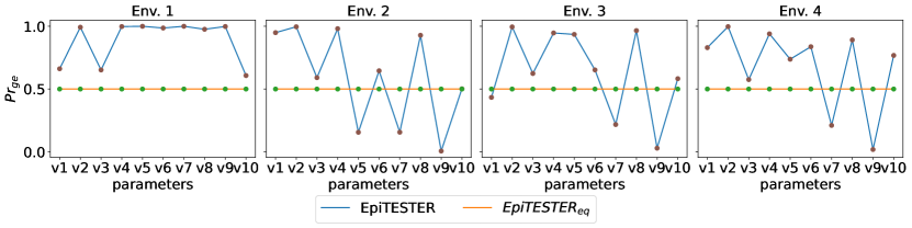
Figure 7: Gene expression probabilities (i.e., $Pr_{ge}$) predicted by the epigenetic model in EpiTESTER (blue) and the default $Pr_{ge}$ applied in $\textit{EpiTESTER}_{eq}$ (orange) – RQ3. v1: $dis^{lo}_{npc}$, v2: $dis^{la}_{npc}$, v3: $behaviour_{npc}$, v4: $dis^{lo}_{ped}$, v5: $dis^{la}_{ped}$, v6: $o^{x}_{ped}$, v7: $o^{y}_{ped}$, v8: $v_{ped}$, v9: $angle_{sun}$, v10: $density_{fog}$.

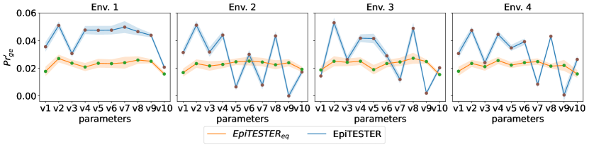
Figure 8: Gene expression probability distributions (i.e., $Pr_{ge}^{\prime}$) of EpiTESTER and $\textit{EpiTESTER}_{eq}$ with 95% confidence intervals – RQ3. v1: $dis^{lo}_{npc}$, v2: $dis^{la}_{npc}$, v3: $behaviour_{npc}$, v4: $dis^{lo}_{ped}$, v5: $dis^{la}_{ped}$, v6: $o^{x}_{ped}$, v7: $o^{y}_{ped}$, v8: $v_{ped}$, v9: $angle_{sun}$, v10: $density_{fog}$.

Conclusion for RQ3: GS mechanism can affect the expression of environmental parameters, and the attention mechanism can effectively identify the contribution of each parameter to collisions or safety violations as the probability of expressing each parameter. Specifically, parameters related to dynamic objects have higher chances of being expressed than weather parameters.

6.4 Threats to Validity

Conclusion Validity concerns the validity and reliability of conclusions drawn in the empirical study. Since EpiTESTER is a search-based AV testing method, to account for the inherent randomness of the search algorithms, we repeated each experiment 10 times – commonly used in other AV testing research [2]. We further executed each obtained solution 30 times to account for the inherent randomness in AV. Following the guidelines from [54], we performed statistical tests to draw solid conclusions.

Construct Validity is related to the metrics used to compare EpiTESTER with the baseline methods. To ensure the fairness of the comparisons, we chose five evaluation metrics commonly used in the context of AV testing and evaluation [46, 58] and applied them consistently to all methods.

Internal Validity concerns our EpiTESTER’s hyperparameter settings. To mitigate the potential threats to the internal validity,we determined the hyperparameter settings by experimenting with different parameter configurations and chose the best one as our hyperparameter setting. We acknowledge that EpiTESTER’s performance might be further improved with more optimized hyperparameter settings; however, this would require dedicated and large-scale empirical studies.

External Validity is about the generalization of the empirical study. We employed one subject system and one simulator to build the test environment, which can potentially threaten the external validity. To mitigate the issue, we chose the state-of-the-art ADS (i.e., Interfuser) that ranked first on the CARLA leaderboard. We acknowledge that conducting more case studies could strengthen our conclusions, and in the future, we plan to explore more simulators and ADS to strengthen our conclusions.

6.5 Data Avalibility

To promote open science, we provide the replication package in an online repository: https://github.com/Simula-COMPLEX/EpiTESTER. Once the paper is accepted, we will release it in a permanent repository, such as Zenodo.

7 Discussions

7.1 Benefiting from attention mechanism

Many environmental parameters can be employed to characterize test scenarios, but not all contribute equally to safety violations. Hence, the attention mechanism in EpiTESTER allows the epigenetic model to dynamically allocate more attention (i.e., lower GS probabilities) to specific parameters that are more likely to lead to safety violations. The epigenetic model can achieve this due to several reasons. First, to better understand the environment, the epigenetic model integrates a multi-modal fusion transformer that leverages a self-attention mechanism to integrate geometric and semantic information from the environment across multiple modalities. This step extracts a high-level feature representation of the environment for the GS probability generation. Second, the self-attention layer for the GS probability generation (Section 4.2.2) allows the epigenetic model to weigh the importance of each environmental parameter in a given environment by calculating attention weights between the word embeddings of the environmental parameters and feature representations of the environmental states. The calculated attention weights determine the contribution of each environmental parameter to the safety violations, which is further used as GS probabilities.

7.2 Incorporating multiple objectives

The current EpiTESTER design considers a single objective (i.e., distance minimization) when generating safety-critical AV test scenarios. In practice, multiple AV testing objectives related to safety and functionality often need to be considered simultaneously. As concluded in Section 6.1, there are correlations between the objective and other metrics: for CO and IS, the correlation is very high, while for RC and DS the correlation is negligible. This observation inspires us to further investigate the multi-objective EpiTESTER design to optimize multiple objectives simultaneously. Considering that some objectives are high-correlated (e.g., MD with CO and IS), one possibility could be deriving one objective by combining these objectives together, e.g., summing them up with equal weights. For others (e.g., MD with RC and DS), multi-objective search algorithms (MOSAs) such as NSGA-II [16] can be applied to solve the optimization problem. However, no algorithms currently combine MOSAs and epigenetics, which calls for future research.

7.3 Investigating other epigenetic mechanisms

In this work, we employ gene silencing (i.e., GS) as the epigenetic mechanism (i.e., EM). In addition to GS, other EMs have also been studied in biology, such as Genomic Imprinting (GI) [61], Paramutation [62], and X-Chromosome Inactivation (XCI) [63]. Implementing these EMs as novel epigenetic operators and integrating them into GAs is interesting to investigate. For instance, GI involves parent-of-origin-specific gene expression patterns – the activity of certain genes is influenced by whether they are inherited from the mother or the father. In the GA context, this could be analogous to assigning different levels of influence (reflected as weights or probabilities) to genes inherited from one parent during optimization, i.e., introducing the concept of ”parental influence” in GAs, where certain parameters are more likely to be inherited from one parent than from the other. Integrating EMs, such as GI, into GAs opens up new possibilities for improving their performance, which we believe is interesting to investigate in the future.

8 Related Work

We discuss relevant works related to scenario-based AV testing (Section 8.1) and epigenetic algorithms (Section 8.2).

8.1 Scenario-Based AV Testing

Various driving scenarios are needed to test how well an AV interacts with the environment and makes proper decisions. However, infinite driving scenarios make it impossible to exhaustively test AV. Thus, we must identify critical scenarios, i.e., scenario-based AV testing [64]. In the literature, a set of search-based testing (SBT) approaches have been proposed [8, 9, 65, 66, 10] and also some reinforcement learning (RL) based AV testing approaches have been proposed as well [12, 67, 11, 2]. There also exist works on generating scenarios from real-world driving data [13, 14, 68].

SBT-based approaches identify critical scenarios where fitness functions guide the optimization process toward generating critical scenarios. For example, NSGAII-SM [8] combines NSGA-II [16] with surrogate models to generate test scenarios for a pedestrian detection vision system. NSGAII-DT [9] tests a vision-based control system combining NSGA-II with decision tree classification models to effectively identify critical scenarios. Considering failures in AV may also originate from unintended interactions among system features (e.g., command conflicts between the automated emergency braking system and the adaptive cruise control system may compromise the AV’s safety), Abdessalem et al. [65] integrated a set of hybrid objectives with a search algorithm to generate critical scenarios. Calò et al. [66] adapted NGSA-II to search for collisions and AV configurations that can avoid such collisions. By combining fuzzing testing and search algorithms, Li et al. [10] developed AV-FUZZER to generate critical scenarios that can identify safety violations of AV. Focusing on testing AV against traffic laws, Sun et al. [69] proposed LawBreaker, which adopts a fuzzing engine to search for scenarios that can effectively violate traffic laws.

RL-based testing approaches identify critical scenarios by dynamically and adaptively exploring the vast parameter space. Chen et al. [67] tests lane-changing models and developed an RL-based adaptive testing framework to generate time-sequential adversarial scenarios. DeepCollision [11] is an RL-based approach that generates safety-critical scenarios by dynamically configuring an AV’s operating environment. By combining RL and multi-objective search, Haq et al. [2] proposed a multi-objective RL approach, MORLOT, for testing AV. MORLOT uses RL to adaptively generate critical scenarios that can cause requirement violations and adopts multi-objective search to cover as many requirements as possible. Feng et al. [12] adapted dense RL, in which the Markov decision process is edited by removing non-safety-critical states, to learn critical scenarios from naturalistic driving data.

Approaches have also been proposed to identify critical scenarios from traffic accident reports and real-world driving data [13, 14]. Gambi et al. [68] proposed AC3R to extract the vehicle crash information from the police reports and recreate the scenario in simulation for testing AVs. Zhang et al. [13] adopted surrogate models in a scenario-based test to expedite the risk assessment of AV, and to fit the naturalistic distribution of the generated scenarios, HighD dataset [70] was applied in their approach. Zhang et al. [71] proposed the M-CPS model to extract information from real-world accidents. Based on the extracted accident information, a mutation testing solution automatically builds critical testing scenarios. To bridge the gap between the simulation and the real-world driving environment, Yan et al. [14] proposed NeuralNDE, which learns naturalistic multi-agent interaction behavior from vehicle trajectory data based on statistical realism.

Different from the existing methods that treat environmental parameters equally when generating critical scenarios, EpiTESTER utilizes a novel attention-based GS mechanism to selectively express parameters with high contribution to safety violations and silence those with low contribution; therefore, compared to the baseline methods (i.e., GA and $\textit{EpiTESTER}_{eq}$), EpiTESTER is more effective and efficient in generating critical scenario generation (Section 6.1 and Section 6.2).

8.2 Epigenetic Algorithm

In the literature, only a few epigenetic algorithms have been proposed. Tanev and Yuta [18] proposed an epigenetic programming approach, i.e., epigenetic learning (EL), incorporating histone modification mechanisms to control gene expression. EpiGA [17] implements GS and integrates it into GA to control how genes are expressed in response to environmental uncertainties. Another work, EpiLearn [20], encodes dynamic environmental changes as an epigenetic layer in a learning process to allow for adaptive and efficient learning. RELEpi [21] supports the coevolving decision-making of groups of agents (swarms) in uncertain environments, but it has not yet proven effective for solving real-world problems. These works demonstrate that epigenetic algorithms are a promising direction for coping with uncertainty, which has also been emphasized in [19].

Our approach EpiTESTER is the first to incorporate epiGA and extend its GS mechanism for addressing AV testing challenges by adopting a transformer model to effectively identify each environmental parameter’s contribution to safety violations as GS probabilities.

9 Conclusion and Future Work

Given infinite driving scenarios, generating critical ones for scenario-based AV testing is practically challenging. In this paper, we propose a novel method, named EpiTESTER, which extends the Gene Silencing (GS) mechanism in epiGA to selectively express or silence certain environmental parameters with GS probabilities. By using an epigenetic model built based on an attention mechanism, the GS probabilities are adaptively generated as the driving environment changes. We evaluate EpiTESTER on a state-of-the-art AV using two comparison baselines, and the experiment results show that EpiTESTER outperformed the baselines in terms of collision scenario generation while guaranteeing a faster convergence speed. In the future, we are interested in studying the generalization of EpiTESTER by conducting experiments with other AVs and simulators. In addition, we plan to investigate other epigenetic mechanisms that can be potentially applied in EpiTESTER, such as histone modifications and genomic imprinting.

References

- [1] C. E. Tuncali, G. Fainekos, H. Ito, and J. Kapinski, “Simulation-based adversarial test generation for autonomous vehicles with machine learning components,” in 2018 IEEE Intelligent Vehicles Symposium (IV), pp. 1555–1562, IEEE, 2018.
- [2] F. U. Haq, D. Shin, and L. C. Briand, “Many-objective reinforcement learning for online testing of dnn-enabled systems,” in Proceedings of the 45th International Conference on Software Engineering, ICSE ’23, p. 1814–1826, IEEE Press, 2023.
- [3] S. Wang and Z. Li, “Exploring the mechanism of crashes with automated vehicles using statistical modeling approaches,” PloS one, vol. 14, no. 3, p. e0214550, 2019.
- [4] F. van Wyk, A. Khojandi, and N. Masoud, “A path towards understanding factors affecting crash severity in autonomous vehicles using current naturalistic driving data,” in Intelligent Systems and Applications: Proceedings of the 2019 Intelligent Systems Conference (IntelliSys) Volume 2, pp. 106–120, Springer, 2020.
- [5] A. A. Kordani, O. Rahmani, A. A. Nasiri, and S. M. Boroomandrad, “Effect of adverse weather conditions on vehicle braking distance of highways,” Civil Engineering Journal, vol. 4, no. 1, pp. 46–57, 2018.
- [6] B. Weinhold, “Epigenetics: the science of change,” 2006.
- [7] E. Gibney and C. Nolan, “Epigenetics and gene expression,” Heredity, vol. 105, no. 1, pp. 4–13, 2010.
- [8] R. Ben Abdessalem, S. Nejati, L. C. Briand, and T. Stifter, “Testing advanced driver assistance systems using multi-objective search and neural networks,” in Proceedings of the 31st IEEE/ACM International Conference on Automated Software Engineering, pp. 63–74, 2016.
- [9] R. B. Abdessalem, S. Nejati, L. C. Briand, and T. Stifter, “Testing vision-based control systems using learnable evolutionary algorithms,” in 2018 IEEE/ACM 40th International Conference on Software Engineering (ICSE), pp. 1016–1026, IEEE, 2018.
- [10] G. Li, Y. Li, S. Jha, T. Tsai, M. Sullivan, S. K. S. Hari, Z. Kalbarczyk, and R. Iyer, “Av-fuzzer: Finding safety violations in autonomous driving systems,” in 2020 IEEE 31st International Symposium on Software Reliability Engineering (ISSRE), pp. 25–36, 2020.
- [11] C. Lu, Y. Shi, H. Zhang, M. Zhang, T. Wang, T. Yue, and S. Ali, “Learning configurations of operating environment of autonomous vehicles to maximize their collisions,” IEEE Transactions on Software Engineering, vol. 49, no. 1, pp. 384–402, 2022.
- [12] S. Feng, H. Sun, X. Yan, H. Zhu, Z. Zou, S. Shen, and H. X. Liu, “Dense reinforcement learning for safety validation of autonomous vehicles,” Nature, vol. 615, no. 7953, pp. 620–627, 2023.
- [13] H. Zhang, H. Zhou, J. Sun, and Y. Tian, “Risk Assessment of Highly Automated Vehicles with Naturalistic Driving Data: A Surrogate-based optimization Method,” in 2022 IEEE Intelligent Vehicles Symposium (IV), pp. 580–585, June 2022.
- [14] X. Yan, Z. Zou, S. Feng, H. Zhu, H. Sun, and H. X. Liu, “Learning naturalistic driving environment with statistical realism,” Nature Communications, vol. 14, no. 1, p. 2037, 2023.
- [15] J. H. Holland, “Genetic algorithms,” Scientific american, vol. 267, no. 1, pp. 66–73, 1992.
- [16] K. Deb, A. Pratap, S. Agarwal, and T. Meyarivan, “A fast and elitist multiobjective genetic algorithm: Nsga-ii,” IEEE transactions on evolutionary computation, vol. 6, no. 2, pp. 182–197, 2002.
- [17] D. H. Stolfi and E. Alba, “Epigenetic algorithms: A new way of building gas based on epigenetics,” Information Sciences, vol. 424, pp. 250–272, 2018.
- [18] I. Tanev and K. Yuta, “Epigenetic programming: Genetic programming incorporating epigenetic learning through modification of histones,” Information Sciences, vol. 178, no. 23, pp. 4469–4481, 2008.
- [19] T. Yue and S. Ali, “Evolve the model universe of a system universe,” in The 38th IEEE/ACM International Conference on Automated Software Engineering (ASE 2023), pp. 1–4, IEEE/ACM, 2023.
- [20] F. Mukhlish, J. Page, and M. Bain, “Reward-based epigenetic learning algorithm for a decentralised multi-agent system,” International Journal of Intelligent Unmanned Systems, vol. 8, no. 3, pp. 201–224, 2020.
- [21] F. Mukhlish, J. Page, and M. Bain, “From reward to histone: Combining temporal-difference learning and epigenetic inheritance for swarm’s coevolving decision making,” in 2020 Joint IEEE 10th International Conference on Development and Learning and Epigenetic Robotics (ICDL-EpiRob), pp. 1–6, IEEE, 2020.
- [22] H. Kellerer, U. Pferschy, D. Pisinger, H. Kellerer, U. Pferschy, and D. Pisinger, Multidimensional knapsack problems. Springer, 2004.
- [23] H. Shao, L. Wang, R. Chen, H. Li, and Y. Liu, “Safety-enhanced autonomous driving using interpretable sensor fusion transformer,” in Conference on Robot Learning, pp. 726–737, PMLR, 2023.
- [24] A. Dosovitskiy, G. Ros, F. Codevilla, A. Lopez, and V. Koltun, “Carla: An open urban driving simulator,” in Conference on robot learning, pp. 1–16, PMLR, 2017.
- [25] V. Bollati and A. Baccarelli, “Environmental epigenetics,” Heredity, vol. 105, no. 1, pp. 105–112, 2010.
- [26] N. Liscovitch-Brauer, S. Alon, H. T. Porath, B. Elstein, R. Unger, T. Ziv, A. Admon, E. Y. Levanon, J. J. Rosenthal, and E. Eisenberg, “Trade-off between transcriptome plasticity and genome evolution in cephalopods,” Cell, vol. 169, no. 2, pp. 191–202, 2017.
- [27] G. Vogt, “Facilitation of environmental adaptation and evolution by epigenetic phenotype variation: insights from clonal, invasive, polyploid, and domesticated animals,” Environmental epigenetics, vol. 3, no. 1, p. dvx002, 2017.
- [28] J. Lämke and I. Bäurle, “Epigenetic and chromatin-based mechanisms in environmental stress adaptation and stress memory in plants,” Genome biology, vol. 18, no. 1, pp. 1–11, 2017.
- [29] R. R. Kanherkar, N. Bhatia-Dey, and A. B. Csoka, “Epigenetics across the human lifespan,” Frontiers in cell and developmental biology, vol. 2, p. 49, 2014.
- [30] J. Bender, “Dna methylation and epigenetics,” Annu. Rev. Plant Biol., vol. 55, pp. 41–68, 2004.
- [31] D. Bahdanau, K. Cho, and Y. Bengio, “Neural machine translation by jointly learning to align and translate,” 2016.
- [32] M.-H. Guo, T.-X. Xu, J.-J. Liu, Z.-N. Liu, P.-T. Jiang, T.-J. Mu, S.-H. Zhang, R. R. Martin, M.-M. Cheng, and S.-M. Hu, “Attention mechanisms in computer vision: A survey,” Computational visual media, vol. 8, no. 3, pp. 331–368, 2022.
- [33] H. Zhang, I. Goodfellow, D. Metaxas, and A. Odena, “Self-attention generative adversarial networks,” in International conference on machine learning, pp. 7354–7363, PMLR, 2019.
- [34] A. Vaswani, N. Shazeer, N. Parmar, J. Uszkoreit, L. Jones, A. N. Gomez, Ł. Kaiser, and I. Polosukhin, “Attention is all you need,” Advances in neural information processing systems, vol. 30, 2017.
- [35] A. Stocco, B. Pulfer, and P. Tonella, “Mind the gap! a study on the transferability of virtual versus physical-world testing of autonomous driving systems,” IEEE Transactions on Software Engineering, vol. 49, pp. 1928–1940, apr 2023.
- [36] D. Ridel, E. Rehder, M. Lauer, C. Stiller, and D. Wolf, “A literature review on the prediction of pedestrian behavior in urban scenarios,” in 2018 21st International Conference on Intelligent Transportation Systems (ITSC), pp. 3105–3112, IEEE, 2018.
- [37] S. Mozaffari, O. Y. Al-Jarrah, M. Dianati, P. Jennings, and A. Mouzakitis, “Deep learning-based vehicle behavior prediction for autonomous driving applications: A review,” IEEE Transactions on Intelligent Transportation Systems, vol. 23, no. 1, pp. 33–47, 2020.
- [38] M. Schimpl, C. Moore, C. Lederer, A. Neuhaus, J. Sambrook, J. Danesh, W. Ouwehand, and M. Daumer, “Association between walking speed and age in healthy, free-living individuals using mobile accelerometry—a cross-sectional study,” PLOS ONE, vol. 6, pp. 1–7, 08 2011.
- [39] B. Chen, X. Chen, Q. Wu, and L. Li, “Adversarial evaluation of autonomous vehicles in lane-change scenarios,” IEEE transactions on intelligent transportation systems, vol. 23, no. 8, pp. 10333–10342, 2021.
- [40] J. W. Ro, P. S. Roop, and A. Malik, “A new safety distance calculation for rear-end collision avoidance,” IEEE Transactions on Intelligent Transportation Systems, vol. 22, no. 3, pp. 1742–1747, 2020.
- [41] M. Bijelic, T. Gruber, and W. Ritter, “Benchmarking image sensors under adverse weather conditions for autonomous driving,” in 2018 IEEE Intelligent Vehicles Symposium (IV), pp. 1773–1779, 2018.
- [42] F. U. Haq, D. Shin, and L. C. Briand, “Many-objective reinforcement learning for online testing of dnn-enabled systems,” in Proceedings of the 45th International Conference on Software Engineering, ICSE ’23, p. 1814–1826, IEEE Press, 2023.
- [43] W. Zhou, J. S. Berrio, S. Worrall, and E. Nebot, “Automated evaluation of semantic segmentation robustness for autonomous driving,” IEEE Transactions on Intelligent Transportation Systems, vol. 21, no. 5, pp. 1951–1963, 2020.
- [44] D. E. Goldberg and K. Deb, “A comparative analysis of selection schemes used in genetic algorithms,” vol. 1 of Foundations of Genetic Algorithms, pp. 69–93, Elsevier, 1991.
- [45] D. E. Goldberg, Genetic Algorithms in Search, Optimization and Machine Learning. USA: Addison-Wesley Longman Publishing Co., Inc., 1st ed., 1989.
- [46] K. Chitta, A. Prakash, B. Jaeger, Z. Yu, K. Renz, and A. Geiger, “Transfuser: Imitation with transformer-based sensor fusion for autonomous driving,” IEEE Transactions on Pattern Analysis and Machine Intelligence, pp. 1–18, 2022.
- [47] A. Rasouli and J. K. Tsotsos, “Autonomous vehicles that interact with pedestrians: A survey of theory and practice,” IEEE Transactions on Intelligent Transportation Systems, vol. 21, no. 3, pp. 900–918, 2020.
- [48] I. Radosavovic, R. P. Kosaraju, R. Girshick, K. He, and P. Dollár, “Designing network design spaces,” 2020.
- [49] O. Levy and Y. Goldberg, “Dependency-based word embeddings,” in Proceedings of the 52nd Annual Meeting of the Association for Computational Linguistics (Volume 2: Short Papers), pp. 302–308, 2014.
- [50] K. He, X. Zhang, S. Ren, and J. Sun, “Deep residual learning for image recognition,” in Proceedings of the IEEE conference on computer vision and pattern recognition, pp. 770–778, 2016.
- [51] A. Prakash, K. Chitta, and A. Geiger, “Multi-modal fusion transformer for end-to-end autonomous driving,” in Proceedings of the IEEE/CVF Conference on Computer Vision and Pattern Recognition, pp. 7077–7087, 2021.
- [52] K. Chitta, A. Prakash, and A. Geiger, “Neat: Neural attention fields for end-to-end autonomous driving,” in Proceedings of the IEEE/CVF International Conference on Computer Vision, pp. 15793–15803, 2021.
- [53] M. R. Endsley, “Autonomous driving systems: A preliminary naturalistic study of the tesla model s,” Journal of Cognitive Engineering and Decision Making, vol. 11, no. 3, pp. 225–238, 2017.
- [54] A. Arcuri and L. Briand, “A practical guide for using statistical tests to assess randomized algorithms in software engineering,” in 2011 33rd International Conference on Software Engineering (ICSE), pp. 1–10, 2011.
- [55] S. Mirjalili and S. Mirjalili, “Genetic algorithm,” Evolutionary Algorithms and Neural Networks: Theory and Applications, pp. 43–55, 2019.
- [56] A. Benítez-Hidalgo, A. J. Nebro, J. García-Nieto, I. Oregi, and J. Del Ser, “jmetalpy: A python framework for multi-objective optimization with metaheuristics,” Swarm and Evolutionary Computation, vol. 51, p. 100598, 2019.
- [57] A. Rácz, D. Bajusz, and K. Héberger, “Effect of dataset size and train/test split ratios in qsar/qspr multiclass classification,” Molecules, vol. 26, no. 4, p. 1111, 2021.
- [58] R. Ben Abdessalem, S. Nejati, L. C. Briand, and T. Stifter, “Testing vision-based control systems using learnable evolutionary algorithms,” in 2018 IEEE/ACM 40th International Conference on Software Engineering (ICSE), pp. 1016–1026, 2018.
- [59] M. M. Mukaka, “A guide to appropriate use of correlation coefficient in medical research,” Malawi medical journal, vol. 24, no. 3, pp. 69–71, 2012.
- [60] E. DESAPRIYA, I. PIKE, M. BRUSSONI, and G. HAN, “The injury severity rate differences in passenger cars and pick up trucks related two vehicle involved motor vehicle crashes in british columbia, canada,” IATSS Research, vol. 28, no. 2, pp. 42–47, 2004.
- [61] W. Reik and J. Walter, “Genomic imprinting: parental influence on the genome,” Nature Reviews Genetics, vol. 2, no. 1, pp. 21–32, 2001.
- [62] R. A. Brink, “Paramutation,” Annual review of genetics, vol. 7, no. 1, pp. 129–152, 1973.
- [63] M. F. Lyon, “X-chromosome inactivation,” Current Biology, vol. 9, no. 7, pp. R235–R237, 1999.
- [64] X. Zhang, J. Tao, K. Tan, M. Törngren, J. M. G. Sánchez, M. R. Ramli, X. Tao, M. Gyllenhammar, F. Wotawa, N. Mohan, M. Nica, and H. Felbinger, “Finding critical scenarios for automated driving systems: A systematic mapping study,” IEEE Trans. Softw. Eng., vol. 49, p. 991–1026, mar 2023.
- [65] R. B. Abdessalem, A. Panichella, S. Nejati, L. C. Briand, and T. Stifter, “Testing autonomous cars for feature interaction failures using many-objective search,” in 2018 33rd IEEE/ACM International Conference on Automated Software Engineering (ASE), pp. 143–154, IEEE, 2018.
- [66] A. Calò, P. Arcaini, S. Ali, F. Hauer, and F. Ishikawa, “Generating avoidable collision scenarios for testing autonomous driving systems,” in 2020 IEEE 13th International Conference on Software Testing, Validation and Verification (ICST), pp. 375–386, IEEE, 2020.
- [67] B. Chen, X. Chen, Q. Wu, and L. Li, “Adversarial evaluation of autonomous vehicles in lane-change scenarios,” IEEE Transactions on Intelligent Transportation Systems, vol. 23, no. 8, pp. 10333–10342, 2022.
- [68] A. Gambi, T. Huynh, and G. Fraser, “Generating effective test cases for self-driving cars from police reports,” in Proceedings of the 2019 27th ACM Joint Meeting on European Software Engineering Conference and Symposium on the Foundations of Software Engineering, pp. 257–267, 2019.
- [69] Y. Sun, C. M. Poskitt, J. Sun, Y. Chen, and Z. Yang, “Lawbreaker: An approach for specifying traffic laws and fuzzing autonomous vehicles,” in Proceedings of the 37th IEEE/ACM International Conference on Automated Software Engineering, ASE ’22, (New York, NY, USA), Association for Computing Machinery, 2023.
- [70] R. Krajewski, J. Bock, L. Kloeker, and L. Eckstein, “The highd dataset: A drone dataset of naturalistic vehicle trajectories on german highways for validation of highly automated driving systems,” in 2018 21st international conference on intelligent transportation systems (ITSC), pp. 2118–2125, IEEE, 2018.
- [71] X. Zhang and Y. Cai, “Building critical testing scenarios for autonomous driving from real accidents,” in Proceedings of the 32nd ACM SIGSOFT International Symposium on Software Testing and Analysis, ISSTA 2023, (New York, NY, USA), p. 462–474, Association for Computing Machinery, 2023.