SparseGS: Real-Time 360° Sparse View Synthesis using Gaussian Splatting

Abstract

The problem of novel view synthesis has grown significantly in popularity recently with the introduction of Neural Radiance Fields (NeRFs) and other implicit scene representation methods. A recent advance, 3D Gaussian Splatting (3DGS), leverages an explicit representation to achieve real-time rendering with high-quality results. However, 3DGS still requires an abundance of training views to generate a coherent scene representation. In few shot settings, similar to NeRF, 3DGS tends to overfit to training views, causing background collapse and excessive floaters, especially as the number of training views are reduced. We propose a method to enable training coherent 3DGS-based radiance fields of 360 scenes from sparse training views. We find that using naive depth priors is not sufficient and integrate depth priors with generative and explicit constraints to reduce background collapse, remove floaters, and enhance consistency from unseen viewpoints. Experiments show that our method outperforms base 3DGS by up to 30.5% and NeRF-based methods by up to 15.6% in LPIPS on the MipNeRF-360 dataset with substantially less training and inference cost.
Our project webpage: https://formycat.github.io/SparseGS-Real-Time-360-Sparse-View-Synthesis-using-Gaussian-Splatting/

0.19 Ground Truth0.20 SparseNeRF0.22 Mip-NeRF 3600.2 3DGS0.21

1 Introduction

The problem of learning 3D representations from 2D images has long been of interest, but has always been a difficult challenge due to the inherent ambiguities in lifting data to higher dimensions. Neural Radiance Fields (NeRFs) [17, 1, 2] tackle this problem by training a neural network using 2D posed images to predict the color and density of points in 3D space. The simplicity and quality of NeRFs enabled significant advances in novel view synthesis and led to a flurry of follow-up work. 3D Gaussian Splatting [11], a more recent technique, builds off of the ideas of NeRFs but replaces the implicit neural network with with an explicit representation based on 3D gaussians. These gaussians are rendered using point-based splatting, which allows for high rendering speeds, but requires fine-grained hyperparameter tuning. While NeRFs and 3D gaussian splatting both perform well at the task of novel view synthesis, they tend to require large sets of training views, which can be difficult due to reasons such as variable lighting conditions, weather-dependent constraints, and logistical complexities. As a result, interest in techniques for few-shot novel view synthesis has grown.

The few-shot view synthesis problem is especially difficult because the inherent ambiguity in learning 3D structure from 2D images is significantly exacerbated: with few-views, many regions of scene have little to no coverage. Therefore, there are many possible incorrect 3D representations that can represent the 2D training views correctly but will have poor results when rendering novel views due to artifacts such as ”floaters” [2], floating regions of high density irregularly positioned through the scene, ”background collapse”, when the background is represented by similar looking artifacts closer to cameras, or holes in the representation. Previous works have tackled this problem through the introduction of constraints that regularize the variation between views or the rendered depth maps. To our knowledge, most recent prior works in this area are built on top of NeRF and as a result are limited by long training times and the inherent black-box nature of neural networks. The lack of transparency poses a notable constraint, preventing a direct approach to the problem at hand. Instead, these challenges are approached indirectly through the use of meticulously designed loss functions and constraints.

In this work, we construct a technique for few-shot novel view synthesis built on top of 3D Gaussian Splatting. The explicit nature of our underlying representations enables us to introduce a key new operation: direct floater pruning. This operation identifies the parts of a rendered image that suffer due to floaters or background collapse and allows us to directly edit the 3D representation to remove these artifacts. As a result, we are afforded greater control over when this operation is applied and how selective it is based on the scene representation during training. We show that this operation provides significant benefits in common view synthesis metrics and allows us to operate on full 360° unbounded scenes, a setting which most current few-shot techniques do not handle.

In addition to this new operator, we leverage recent advances in image generation diffusion models to provide supervision in regions with little coverage from training views and apply depth constraints similar to prior work. Together, we show that these techniques can enable high-quality novel-view synthesis from sparse views that out-performs prior state of the art work.

1.1 Contributions

In summary, we make the following contributions:

1. We propose a novel technique for training coherent, robust 3D Gaussian representations from few-views in unbounded 360° settings.

2. We introduce a new explicit, adaptive operator on 3D representations to prune unwanted ”floater” artifacts in point-based 3D representations.

3. We show that our technique provides 30.5% improvments over base 3DGS and 15.6% improvements over NeRF-based methods in LPIPS for few-shot novel view synthesis while running at real-time.

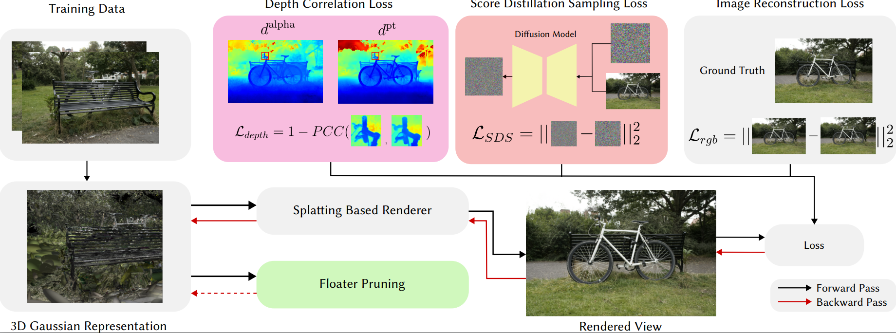
Figure 1: Our proposed pipeline incorporates depth and diffusion constraints along with a floater pruning technique to improve few-shot novel view synthesis performance. During training, we render the alpha-blended depth $d^{\text{alpha}}$ and use Pearson correlation to encourage it to align with $d^{\text{pt}}$ as described in Sec. 3. Additionally, we generate novel views using the procedure described in Sec. 3 and incorporate a score distillation sampling loss. At pre-set intervals, we prune floaters as described in Sec. 3. New components we propose are colored while the base 3D Gaussian Splatting pipeline is in grey.

2 Related Work

Radiance Fields

Radiance Fields, 3D representations of radiance in a scene, were first introduced by Neural Radiance Fields [17] (NeRFs) which represent 3D scenes with a neural volumetric representation that learns a density and color for every point. If density is represented by $\sigma$ and color as $c$, the final color of a ray can be written using volumetric rendering principles as a combination of the density and color at the sample points along the ray as follows:

$$C=\sum_{i}T_{i}\sigma_{i}c_{i}$$ (1)

where $T_{i}$ is the transmittance representing the probability of getting to sample point without intersecting a particle before. NeRFs are then trained using gradient descent on an image reconstruction loss. NeRFs have encouraged a flurry of follow-up work for extending NeRFs with new types of data [18, 12], improving speed [19] or quality [1], or applying them to novel tasks [42, 38]. A set of NeRF follow-ups that are particularly relevant to our topic are Mip-NeRF [1] and Mip-NeRF 360 [2]. Mip-NeRF [1] introduced the concept of anti-aliasing to NeRFs by rendering conical frustums rather than just single rays. As a result, they are able to anti-alias their renders and render at multiple resolutions at high quality. Mip-NeRF 360 was a follow-up work to Mip-NeRF that specifically tackled the problem of representing 360° unbounded scenes. We also focus on this setting in this work as it is a challenging setting for sparse view techniques.

While NeRFs rely on a neural network to represent the radiance field, 3D Gaussian Splatting [11], is a recent technique for view synthesis that replaces the neural network with explicit 3D Gaussians. These gaussians are parameterized by their position, rotation, scaling, opacity, and a set of spherical harmonics coefficients for view-dependent color. They are then rendered by projecting the gaussians down to the image plane using splatting-based rendering techniques [45, 46] and then alpha blending the resulting colors and opacities. Models trained using the same reconstruction loss as NeRFs. Replacing ray-tracing and neural network process of NeRF-based methods with splatting and direct representation process offers significant run-time improvements and allows for real-time rendering during inference. In addition, 3D Gaussian representations are explicit rather than the implicit representations of NeRFs, which allows for more direct editing and easier interpretability. We leverage this property for our technique which identifies and directly deletes floaters.

Recent works have built on top of 3D gaussian splatting to perform a variety of downstream tasks including text-to-3d generation [34, 41], dynamic scene representation [15, 39], and animating humans [44]. However, to our knowledge, we are the first to provide a technique for few-shot novel view synthesis using 3D gaussians.

Few Shot Novel View Synthesis

The problem of novel view synthesis from few images has received significant interest as many view synthesis techniques can require a prohibitively high number of views for real-world usage. Many early techniques [35, 43, 30] leverage multi-plane images (MPIs), which represent images by sub-images at different depths, to re-render depth and color from novel view points using traditional transformations. More recent techniques are built on top of the NeRF framework and tend to tackle the problem one of two ways: The first set of methods introduce constraints on the variation between views. An early example of this type of method was DietNeRF [8] which added constraints to ensure that high-level semantic features remained the same from different views since they contained the same object. Another example is RegNeRF [20] which applies both color and depth consistency losses to the outputs at novel views. ViP-NeRF [29] modifies the traditional NeRF framework to additionally compute the visibility of a point and then uses these outputs to regularize the visibility and alpha-blended depth of different views. The second set of methods approach the problem by adding depth priors to novel views to regularize outputs. SparseNeRF [36] falls into this category and uses a pre-trained depth estimation model to get psuedo-ground truth depth maps which are then used for a local depth ranking loss. They additionally apply a depth smoothness loss to encourage rendered depth maps to be piecewise-smooth. DSNeRF [3] also uses additional depth supervision, but uses the outputs of the SfM pipeline (typically COLMAP [28, 27]) used to get camera poses instead of a pre-trained model. Beyond these two techniques, some prior works approach the problem through recent machine learning techniques. Specifically, Neo 360 [7] uses a tri-plane feature representation to enable their model to reason about 3D features more robustly. To our knowledge, this is also the only other technique that explicitly tackles the problem of 360°few-shot novel-view synthesis.

3 Methods

Our method is comprised of multiple components designed to function cohesively to improve view consistency and depth accuracy for novel views. There are three key components: a depth correlation loss, a diffusion loss, and a floater pruning operation.

Rendering Depth from 3D Gaussians

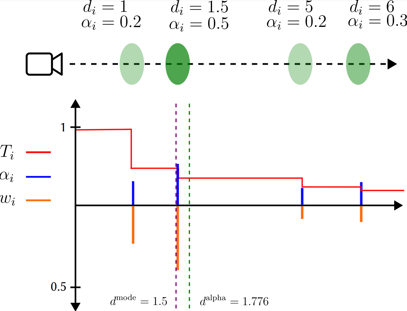
Figure 2: An illustration of how $d^{\text{alpha}}$ and $d^{\text{mode}}$ can disagree. On top, we see an example ray with 4 gaussians along it. On bottom, we see values of $T_{i}$, $\alpha_{i}$, and $w_{i}$ along this ray. Note the upward and downward axes both represent positive values and are shown this way to reduce clutter. The low opacity gaussians far out pull the alpha-blended depth back slightly, leading to ambiguity about the true depth. With more gaussians along a ray, this problem can be exacerbated.

Many of the components we introduce rely on depth maps rendered from the 3D Gaussian representation. In order to compute these, we utilize two techniques: alpha-blending, and mode-selection. Alpha-blending renders depths maps by following the same procedure used for rendering color images. If $d^{\text{alpha}}_{x,y}$ is the alpha-blended depth at a pixel x, y, we can calculate it as:

$$d^{\text{alpha}}_{x,y}=\sum_{i}^{N}T_{i}\alpha_{i}d_{i}$$ (2)

where $T_{i}$ is the accumulated transmittance and $\alpha_{i}$ is the alpha-compositing weight. In mode-selection, the depth of the gaussian with the largest contributing $w_{i}=T_{i}\alpha_{i}$ represents the depth of that pixel. The mode-selected depth of a pixel can be written as:

$$d^{\text{mode}}_{x,y}=d_{\arg\max_{i}\left(w_{i}\right)}$$ (3)

Intuitively, the mode-selected depth can be thought of as choosing the first high opacity gaussian while the alpha blended depth considers almost all gaussians along an imaginary ray from the camera. A key insight that we will rely on later to build our pruning operator is that $d^{\text{mode}}$ and $d^{\text{alpha}}$ are not always the same even though they should be in most ideal settings. An illustration of this is shown in Fig. 2. Here, we have 4 gaussians along a ray, each at varying depths and with varying opacities. At first, $T$ starts at 1. As a reminder $w_{i}=T_{i}\alpha_{i}$ and $T_{i}=T_{i-1}(1-\alpha_{i-1})$ and $T_{0}=1$. Working through the math, we can clearly see that the max value of $w_{i}$ is at the second gaussian where $w_{i}=0.4$. Therefore, $d^{\text{mode}}=1.5.$ However, if we compute all $w_{i}$ values and take the weighted sum of depths, we get:

$$d^{\text{alpha}}=(0.2)(1)+(0.4)(1.5)+(0.08)(5)\\ +(0.096)(6)=1.776$$ (4)

The alpha-blended depth is slightly behind the mode-selected depth due to the low opacity gaussians pulling it to either side. This leads to ambiguity about which is the true depth. We interpret this ambiguity as a measure of the uncertainty of 3DGS at a point and use it to inform our pruning operator introduced later.

We additionally compute a psuedo-ground truth depth map using a pre-trained depth estimation model on top of the training views. We use Monodepth [16, 31] but any pre-trained depth estimation model [23, 24] can work. We refer to the depth from this model as $d^{pt}$ for pre-trained.

Patch-based Depth Correlation Loss

Since the monocular estimation model predicts relative depth while our alpha-blended and mode-based depths are in COLMAP-anchored depth, directly applying a loss such as mean squared error (MSE) would not work well. One option is to attempt to estimate scale and shift parameters and use those to align the two depth maps in metric space. However, the transformation between the depth maps is not guaranteed to be constant at all points, meaning a naive alignment could introduce additional unwanted distortion. Instead, we propose utilizing Pearson correlation across image-patches to compute a similarly metric between depth maps. This is similar to the depth ranking losses proposed by prior work, but instead of comparing two selected points per iteration, we compare entire patches, meaning we can affect larger portions of the image at once and can learn more local structure. The pearson correlation coefficient is the same as normalized cross correlation, so this loss encourages patches at the same location in both depths maps to have a high cross correlation value irrespective of the range of depth values.

At each iteration, we randomly sample $N$ non-overlapping patches to compute the depth correlation loss as:

$$\mathcal{L}_{depth}=\frac{1}{N}\sum^{N}_{i}1-PCC(p^{\text{alpha}}_{i},p^{\text{pt}}_{i})$$ (5)

$$PCC(X,Y)=\frac{\mathbb{E}[XY]-\mathbb{E}[X]\mathbb{E}[Y]}{\sqrt{\mathbb{E}[Y^{2}]-\mathbb{E}[Y]^{2}}\sqrt{\mathbb{E}[X^{2}]-\mathbb{E}[X]^{2}}}$$ (6)

where $p^{\text{alpha}}_{i}\in\mathbb{R}^{S^{2}}$ denotes the $i$th patch of $d^{\text{alpha}}$and $p^{\text{pt}}_{i}\in\mathbb{R}^{S^{2}}$ denotes the $i$th patch of $d^{\text{pt}}$ with the patch size $S$ being a hyper-parameters. Intuitively, this loss works to align the alpha-blended depth maps of the gaussian representation with the depth map of monodepth while avoiding the problem of inconsistent scale and shift.

Score Distillation Sampling Loss

In the few-shot setting, our input training data is sparse and therefore it is likely that we do not have full coverage of our scene. Therefore, inspired by recent advancements in image generative models [34, 26, 5, 21, 9, 40], we propose using a pre-trained generative diffusion model to guide the 3D gaussian representation via Score Distillation Sampling (SDS) as introduced in [22]. This allows us to ”hallucinate” plausible details for regions that do not have good coverage in the training views and generate more complete 3D representations [14, 6, 13, 32]. Our implementation starts by generating novel camera poses within the camera-to-world coordinate system. Specifically, the up-vector of each camera is extracted as

$$Y=\begin{bmatrix}R_{11}\\ R_{21}\\ R_{31}\end{bmatrix}$$ (7)

, with $R$ denoting the rotation matrix. Following this, we compute the normalized average up-vectors across all cameras, serving as an estimation of the scene center. We then create novel viewpoints by rotating the camera center of the current view around this estimated center axis by various degrees using Rodrigues’ rotation formula [25].

$$\bar{Y}=\frac{1}{N}\sum_{i}Y_{i}$$ (8)

$$\bar{Y}=\frac{\bar{Y}}{||\bar{Y}||}$$ (9)

$$P^{\prime}=P\cos{\theta}+(P\times\bar{Y})\sin{\theta}+\bar{Y}(\bar{Y}\cdot P)(1-\cos{\theta})$$ (10)

where $P$ is the original camera pose and $\bar{Y}$ is the estimated up-axis at the scene center. $\theta$ is randomly chosen between a preset interval. Subsequently, random noise is introduced to the rendered image at the novel poses and diffusion model is then used to predict the original image. As the diffusion model is trained on a large-scale dataset and contains general image priors, we expect it to be able to interpolate missing details with plausible pixel values. In practice, we ask the model to predict the noise added to the image rather than the image itself, and the difference between the introduced and the predicted noise then acts as guidance for the 3D Gaussian representation. Mathematically, the guidance loss is formulated as:

$$\hat{I}=\mathcal{N}(\sqrt{\hat{\alpha}}I^{\prime},(1-\hat{\alpha})\mathbf{I})$$ (11)

$$\mathcal{L}_{SDS}=\nabla_{G}\mathbb{E}[(\epsilon_{\phi}(\hat{I}_{p};\tilde{I_{p}})-\epsilon)\frac{\partial\hat{I_{p}}}{\partial G}]$$ (12)

where $G$ represents the parameters of our gaussian representation, $\hat{a}$ represents the cumulative product of one minus the variance schedule and $\epsilon$ is the noise introduced by the SDS, $\epsilon_{\phi}(\cdot)$ is the predicted noise by Stable Diffusion, $\hat{I}_{p}$ is the rendered image at camera pose $p$ with added noise, and $\tilde{I_{p}}$ is the image denoised by Stable Diffusion. Intuitively, the SDS loss first finds the error between the true noise added to an image and the error the diffusion model estimates and then takes the gradient of this error with respect to the parameters of our gaussian model, i.e. the means, scalings, rotations, and opacities of the gaussians.

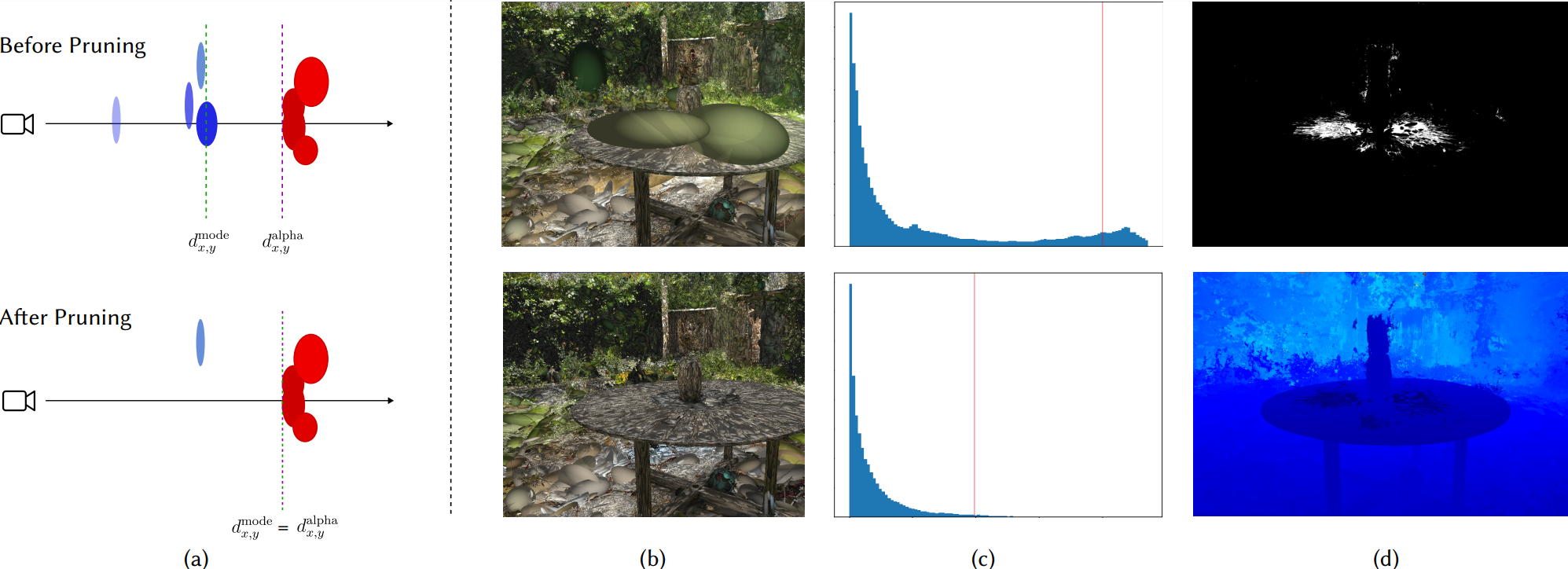
Figure 3: The proposed floater pruning technique removes gaussians at inaccurate depths. A toy example (a) demonstrates the pruning technique: before pruning, there are floaters (shown in blue) in front of the gaussians at the object surface (in red) and therefore, $d_{x,y}^{\text{mode}}$ $d_{x,y}^{\text{alpha}}$ are not aligned. The pruning technique removes all gaussians on that pixel before the mode and as a result, $d_{x,y}^{\text{mode}}=d_{x,y}^{\text{alpha}}$. Applied to the garden scene (b), the pruning technique removes both large floaters in center of the scene and left of the table. We see the link between the bimodality of the histogram of relative differences before and after the pruning operator in (c), with the appropriate pruning cutoff points indicated by the red vertical line. (d) top: The floater mask $F_{i}$ is obtained from thresholding the relative differencing of the mode depth $d^{\text{mode}}$ (bottom) at the cutoff points.

Floater Removal

Function prune_floaters$(G,P,a,b)$

       Input : Gaussian Representation $G$

       Input : Camera Poses $P$

       Input : Curve Parameters $a,b$

       $\bar{D}\leftarrow 0.0$

       foreach $p\in P$ do

             $d^{\text{alpha}}\leftarrow$ alpha_blend_depth($G,p$)

             $d^{\text{mode}}\leftarrow$ mode_select($G,p$)

             $\Delta_{p}\leftarrow\frac{d^{\text{mode}}-d^{\text{alpha}}}{d^{\text{alpha}}}$

             $\bar{D}\leftarrow\bar{D}+$ dip_test($\Delta_{p}$)

            

       end foreach

      $\bar{D}\leftarrow\bar{D}/|P|$

       foreach $p\in P$ do

             $\tau_{p}\leftarrow\text{percentile}(\Delta_{p},ae^{b\bar{D}})$

             $F_{p}\leftarrow\mathbb{1}[\Delta_{p}>\tau]$

             ${g_{0},g_{1},...,g_{n}}\leftarrow$ mask_to_gaussian($F_{p}$)

             remove_gaussians(${g_{0},g_{1},...,g_{n}}$)

            

       end foreach

      

end

ALGORITHM 1 Algorithm to prune floaters

Although the model is trained with the depth correlation loss, optimizing the alpha-blended depth alone does not solve the problem of ”floaters”. As seen in Fig. 1 An example image with floaters is shown in Fig. 3b. In order to remove floaters, we propose a novel operator which leverages the explicit representation of 3D gaussians to remove floaters and encourage the model to re-learn those regions of the training views correctly. ”Floaters” often manifest themselves as relatively high opacity gaussians positioned close to the camera plane. As a result, although they do not appear prominently when we render the alpha-blended depth of a scene because they are ”averaged” out, they are prominent in the mode-selected depth. We leverage this difference to generate a floater mask $F$ for each training view. Having identified this mask in image space, we then select and prune all gaussians up-to and including the mode gaussian. Specifically, we compute $F$ for a single training view $i$ as follows: we first compute $\Delta_{i}$, the relative difference between the mode-selected depth and alpha-blended depth. When visualizing the distributions of $\Delta_{i}$, we noticed that images with many floaters had bi-modal histograms, as floaters tend to be far from the true depth, while images without floaters tended to be more uni-modal. We visualize this phenomenon in Fig. 3. Leveraging this, we perform the dip test [4], a measure of uni-modality, on the distribution. We then average the uni-modality score across all training views for a scene, since the number of floaters is generally a scene wide metric, and use the mean to select a cut-off threshold for the relative differences. The dip statistic to threshold conversion process is performed using an exponential curve with parameters $a,b$. We estimate these parameters by manually examining $\Delta_{i}$ and $F_{i}$ for various scenes from different datasets and real world capture. This process was carefully designed to allow our floater pruning to be adaptive: in some cases, our 3D scenes are already quite high quality and as a result do not have many floaters. In that situation, if we set a pre-defined threshold for the percent of pixels to prune, we would be forcing ourselves to delete detail from the scene. Similarly, some scenes are especially difficult to learn (due to the 3D structure or distribution of training images) and in those cases, we would like our pruning to remove more floaters than normal. The average dip score $\bar{D}$ provides a proxy measure of how many floaters a scene contains and allows us to adjust our techniques in response. Our full pruning process is visualized in Fig. 3 and shown in Algorithm 1. Mathematically, our process can be written as:

$$\Delta_{i}=\frac{d^{\text{mode}}_{i}-d^{\text{alpha}}_{i}}{d^{\text{alpha}}_{i}}$$ (13)

$$\bar{D}=\frac{1}{N}\sum_{i}D(\Delta_{i})$$ (14)

$$\tau=\text{percentile}(\Delta_{i},ae^{b\bar{D}})$$ (15)

$$F_{i}=\mathbb{1}[\Delta_{i}>\tau]$$ (16)

Full Loss

Combined, our full loss is:

$$\mathcal{L}=\mathcal{L}_{rgb}(\hat{I},I)+\lambda_{depth}\mathcal{L}_{depth}(d^{\text{alpha}},d^{\text{pt}})\\ +\lambda_{SDS}\mathcal{L}_{SDS}(\hat{I}^{\prime})$$ (17)

where $\hat{I}$ is the rendered image, $I$ is the ground truth image, and $\hat{I}^{\prime}$ is a rendered image from a random novel viewpoint (not a training view). $\mathcal{L}_{rgb}$ is the same loss as is used to train 3D Gaussian Splatting.

4 Results

Mip-NeRF 360 Dataset

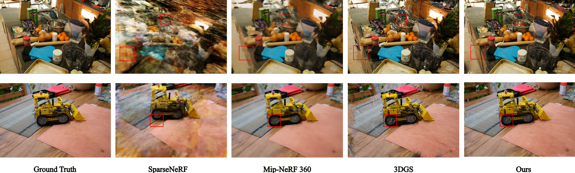
Figure 4: Qualitative results from the Mip-NeRF 360 dataset show our model produces images that are sharper and perceptually similar to ground truth. Red boxes show specific regions of interest. Our model is able to reconstruct high-frequency detail such as the tires of the lego bulldozer and the plates while also maintaining coherence across the full image.

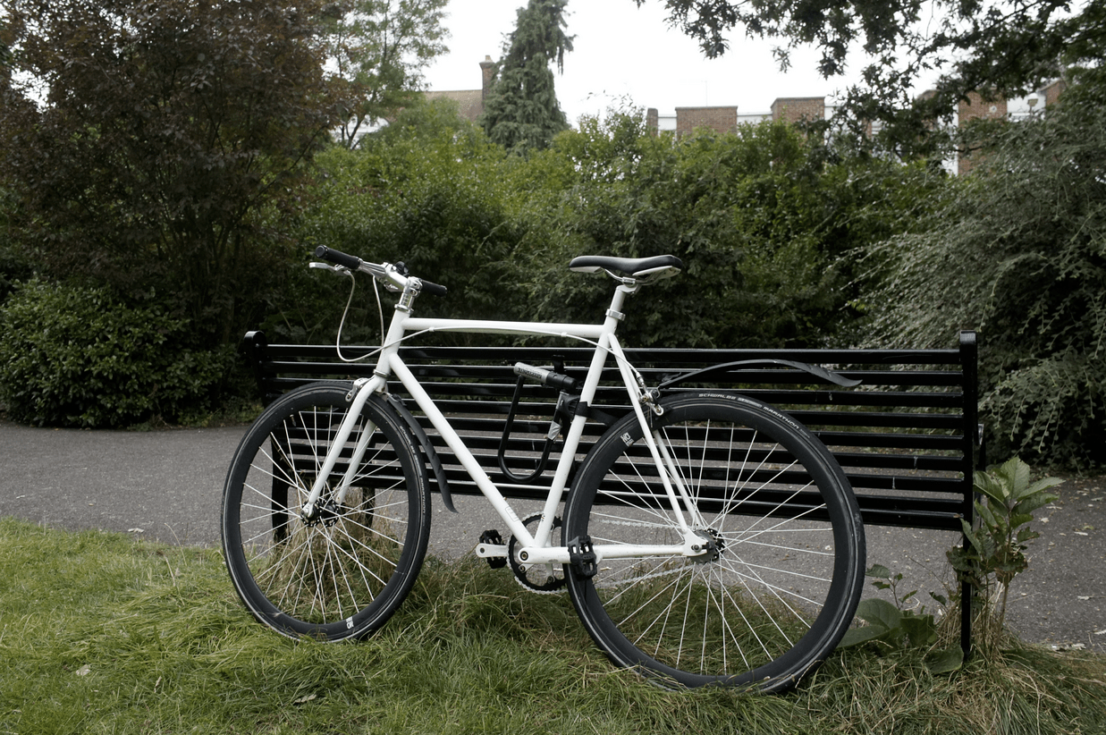
(a)

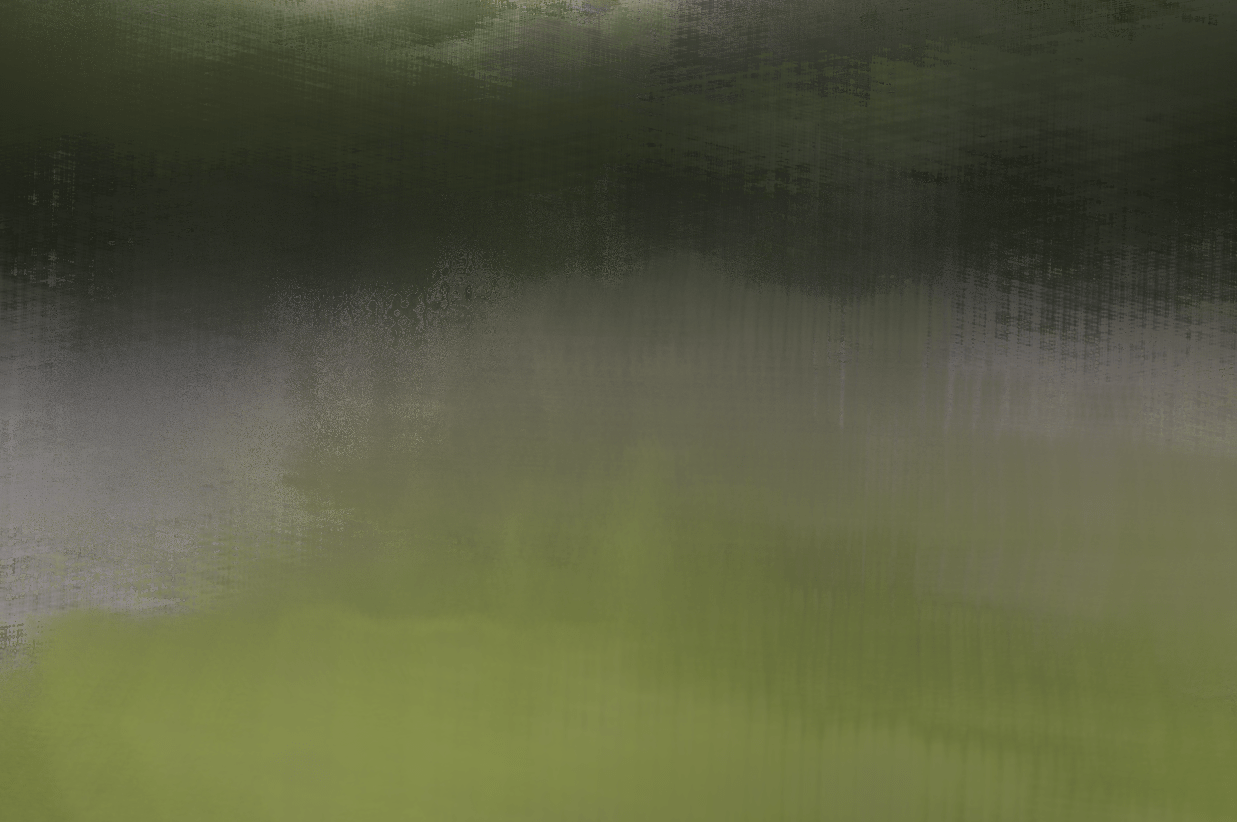
(b)

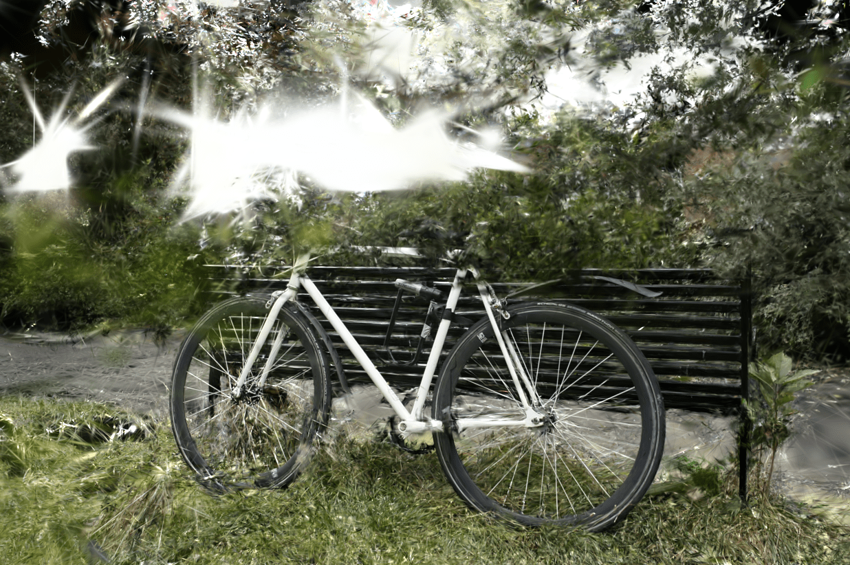
(c)

(d)

Figure 5: Our model visually outperforms DSNeRF for few-shot view synthesis. Renders from DSNeRF can often be overly smooth due to the inherent nature of neural networks. Our representation is high quality in the scene center where we have high coverage, but can lose quality in the edges of an image.

Since our technique is focused on unbounded, 360° scenes, we evaluate on the Mip-NeRF 360 dataset designed specifically for this use case. The full dataset contains 9 scenes, but we select 6 of them which truly have 360° coverage. We compare against Mip-NeRF 360 [2], DSNeRF [3], SparseNeRF [36], and base 3D Gaussian Splatting [11]. DSNeRF and SparseNeRF are specifically designed for the few-shot setting, but are focused on frontal scenes. Mip-NeRF 360 and 3D Gaussian Splatting are designed for the general view synthesis case, but are also designed to handle 360° scenes. Thus, we use them as comparison benchmarks in our evaluation.For this setting, we use 12 views. Results on PSNR, SSIM, and LPIPS are shown in Tab. D and Tab. 2. We additionally compare the runtimes of all methods. We opted to split the evaluation into two tables due to limitations in memory: running DSNerf at higher resolutions was not possible within these constraints. On the higher resolution comparison (against Mip-NeRF 360, SparseNeRF, etc..), we outperform all baselines on SSIM and LPIPS and are competitive on PSNR. For LPIPS specifically, we are 15.6% lower than the next best performing technique, Mip NeRF 360. We see a similar pattern for our comparison against DSNeRF where we outperform DSNeRF by 52.6%. Additionally, our technique trains in less than an hour and can run inference in real-time (30+ FPS). Across both comparisons however, we are outperformed on PSNR. We believe this to be a result of the specific failure modes of our technique: NeRF based methods tend to face the problem of having outputs that are too smooth, which was what originally prompted the introduction of the positional encoding  [17, 33]. As a result, in these few-shot settings, the renders from NeRF exhibit an overly smooth appearance. Conversely, the 3D gaussian representation gravitates towards positioning isolated gaussians in regions of empty space. As a result, when our model does not have a good representation of a scene region, we end up with high-frequency artifacts. PSNR tends to tolerate overly smooth outputs while heavily penalizing high-frequency artifacts [37], leading to the poor performance of our model when compared to NeRF baselines. On a perceptual metric such as LPIPS, we significantly outperform the next closest baseline.

Model	PSNR $\uparrow$	SSIM $\uparrow$	LPIPS $\downarrow$	Runtime (h)	Render FPS
SparseNeRF	11.5638	0.3206	0.6984	4	1/120
Base 3DGS	15.3840	0.4415	0.5061	0.5	30
Mip-NeRF 360	17.1044	0.4660	0.5750	3	1/120
Ours	16.6898	0.4899	0.4849	0.75	30

Table 1: Our model out-performs previous SOTA for few-shot novel view synthesis on all but one metric (PSNR) when tested on the Mip-NeRF 360 dataset. Runtimes are recorded on 1 RTX3090.

Model	PSNR $\uparrow$	SSIM $\uparrow$	LPIPS $\downarrow$	Runtime (h)	Render FPS
DSNeRF	17.4934	0.3620	0.6242	4	1/50
Base 3DGS	15.2437	0.3914	0.4824	0.5	40
Ours	16.1882	0.4198	0.4671	0.75	40

Table 2: Our model out-performs previous SOTA on SSIM and LPIPS for few-shot novel view synthesis on the Mip-NeRF 360 dataset. Results in this table were rendered at 1/4x resolution due to memory constraints with DSNeRF. All models were run at the same resolution for fairness. Runtimes were recorded on 1 RTX3090

Ablation Studies

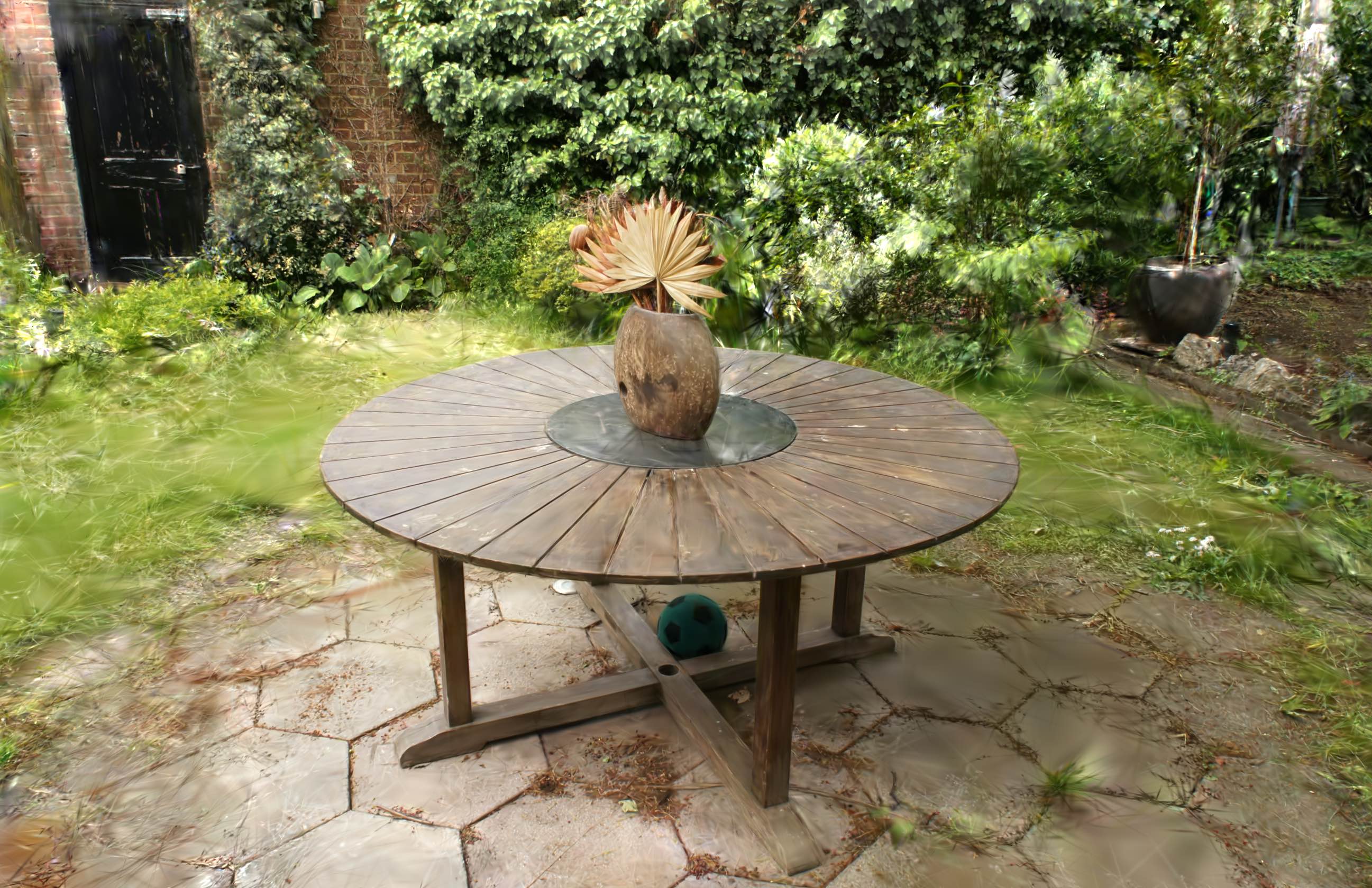
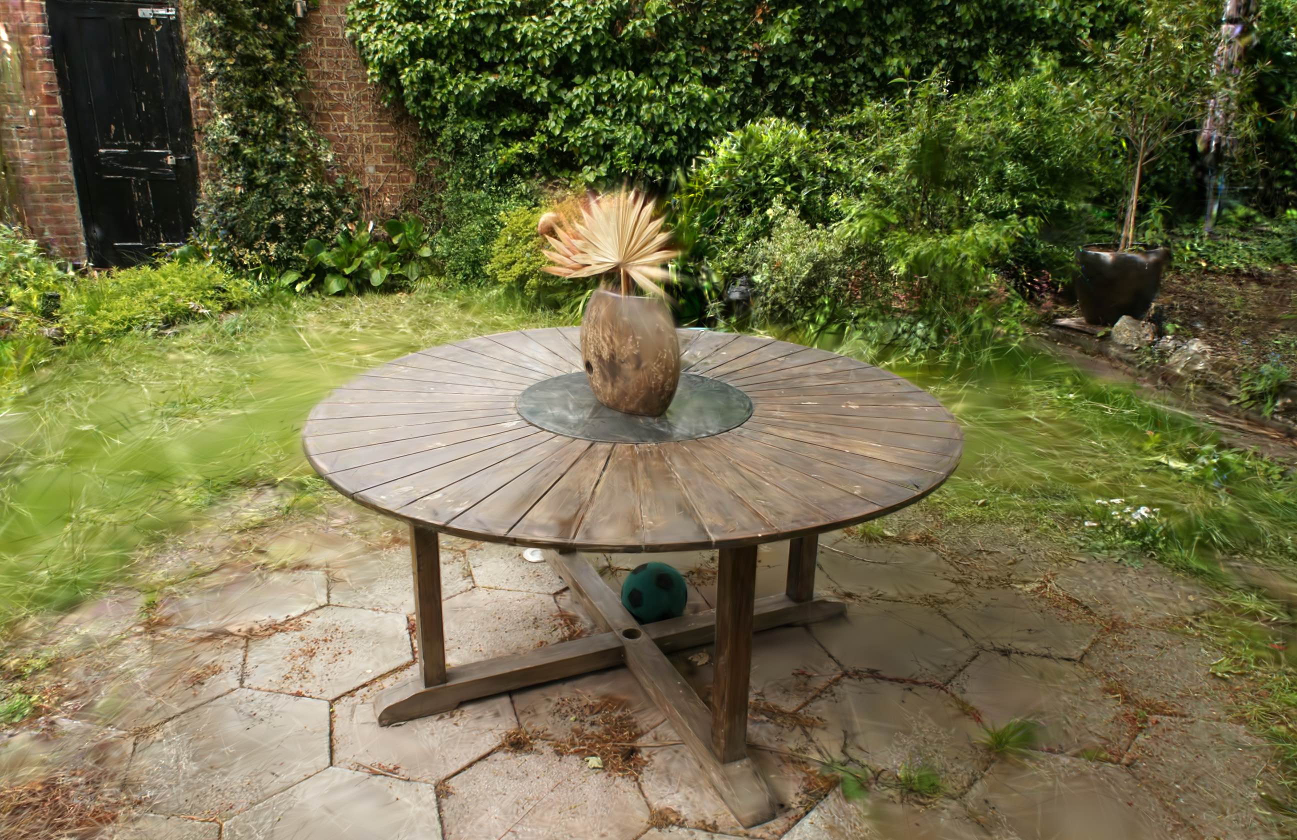
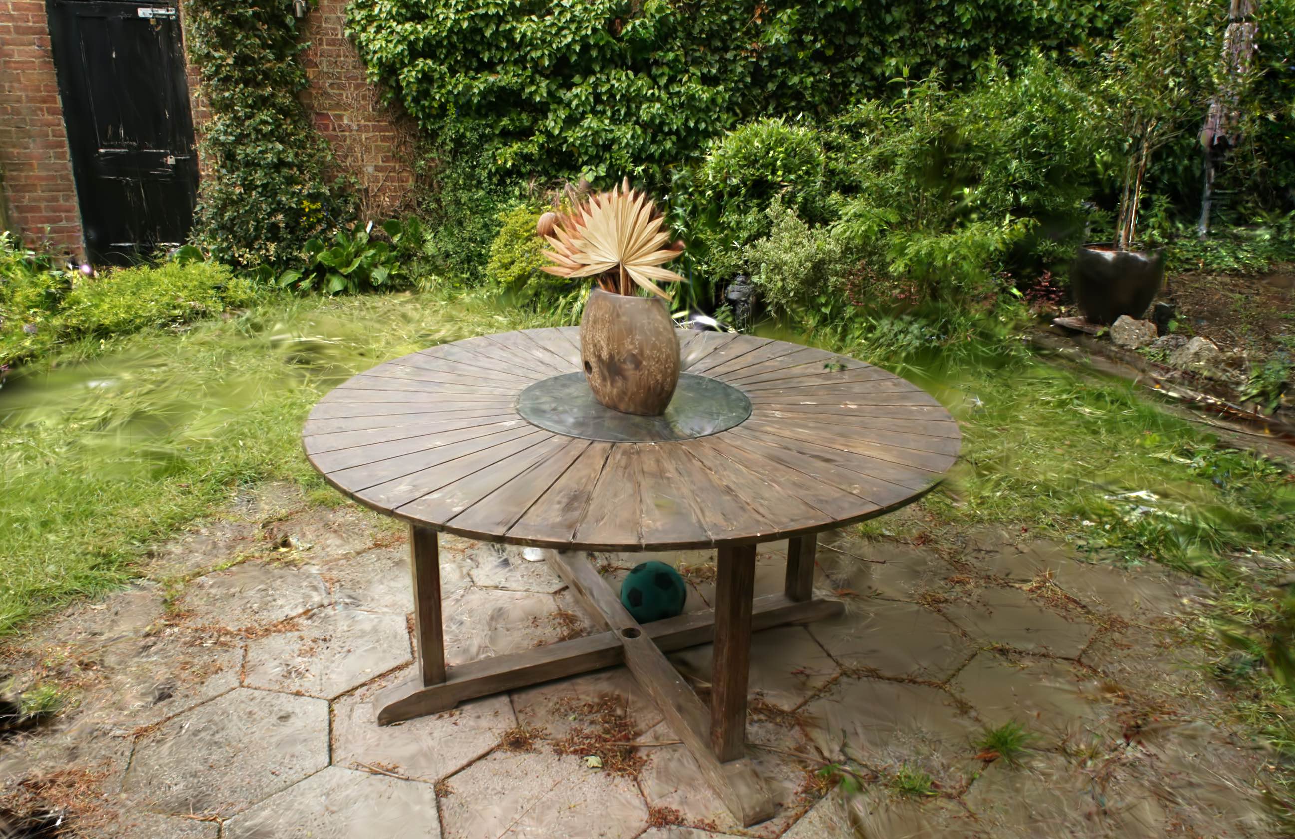
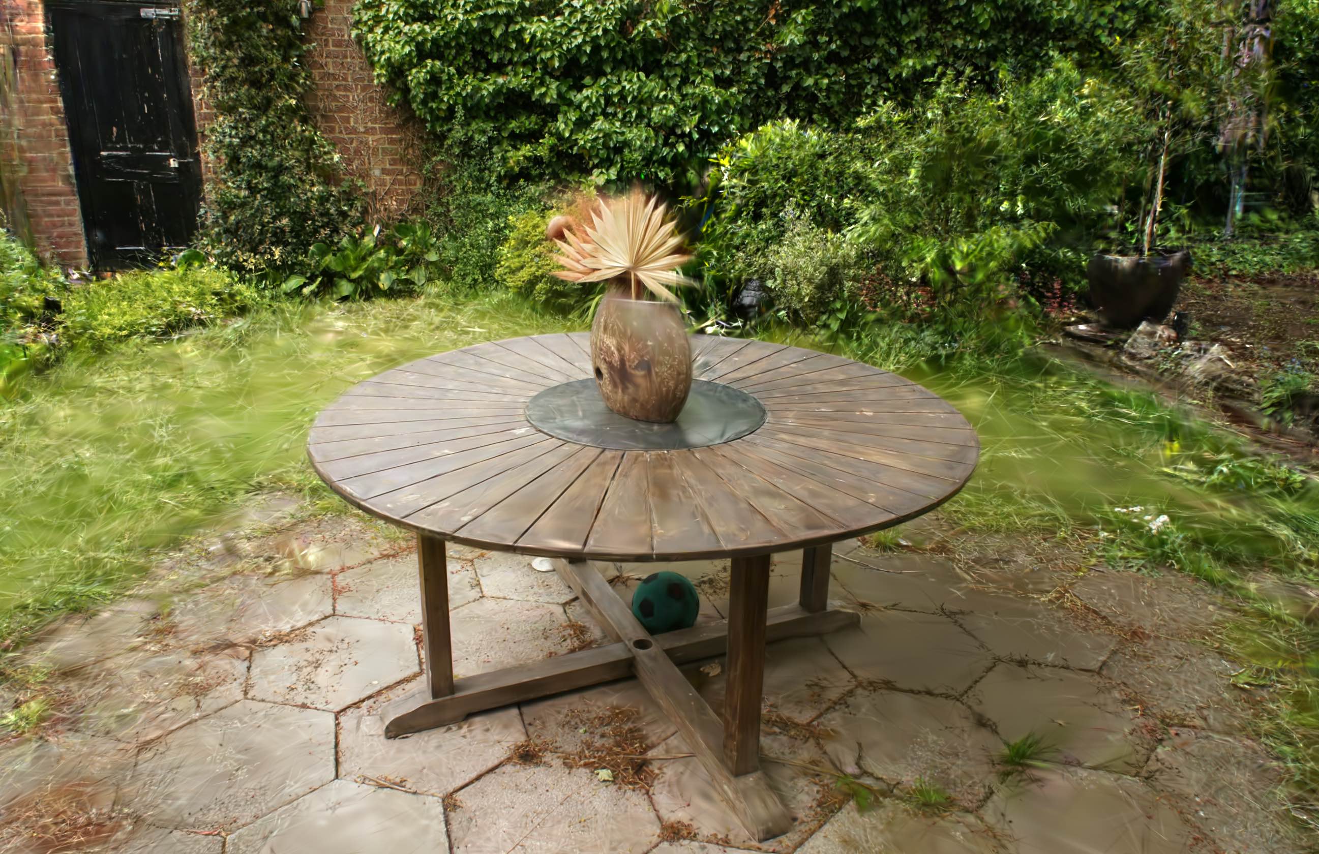
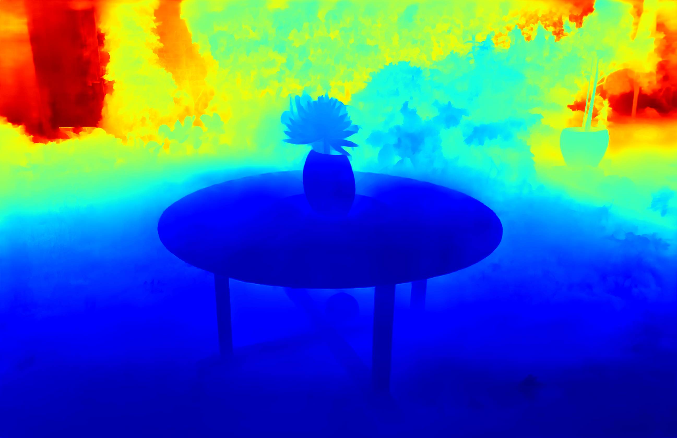
(a)

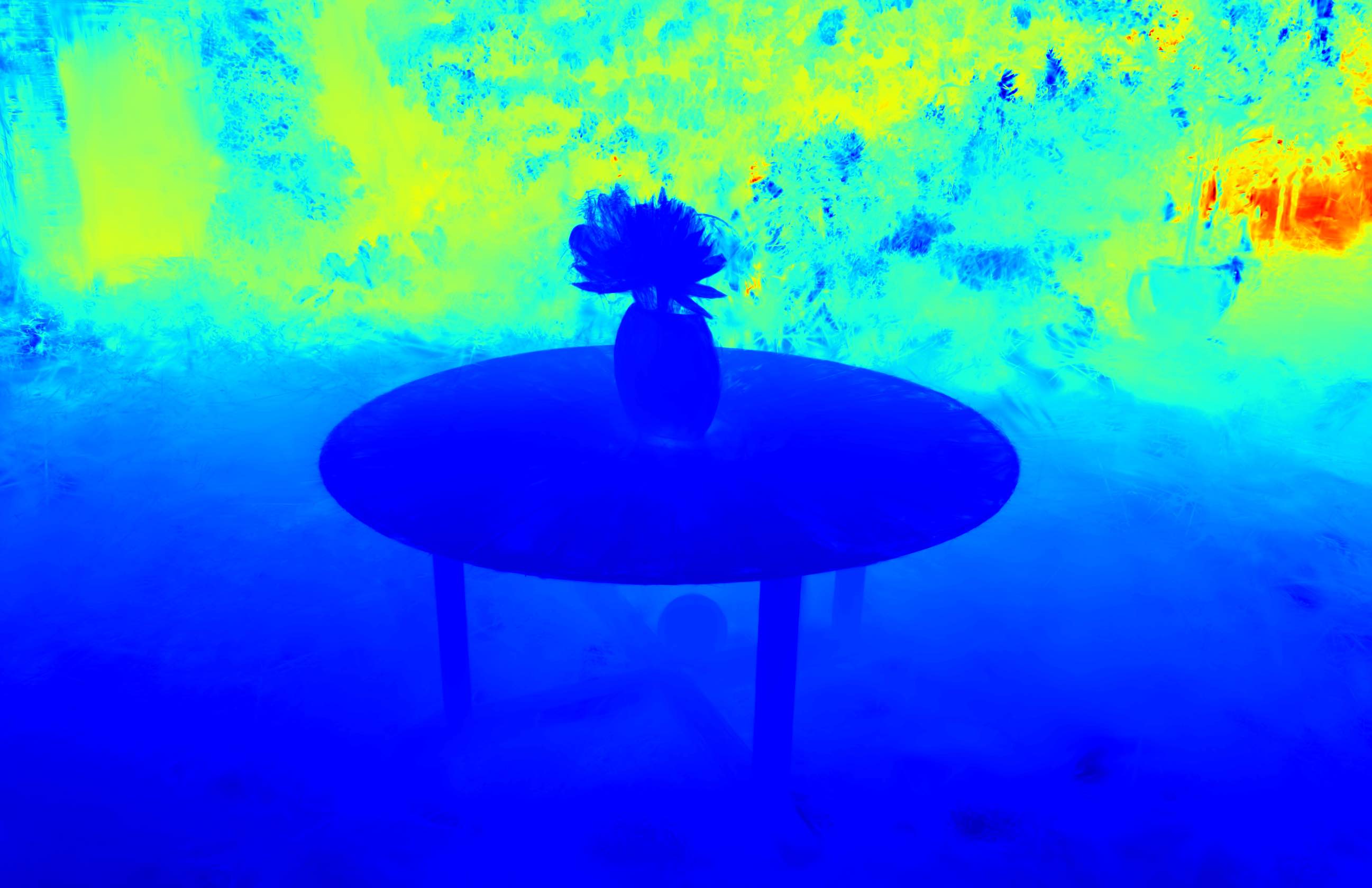
(b)

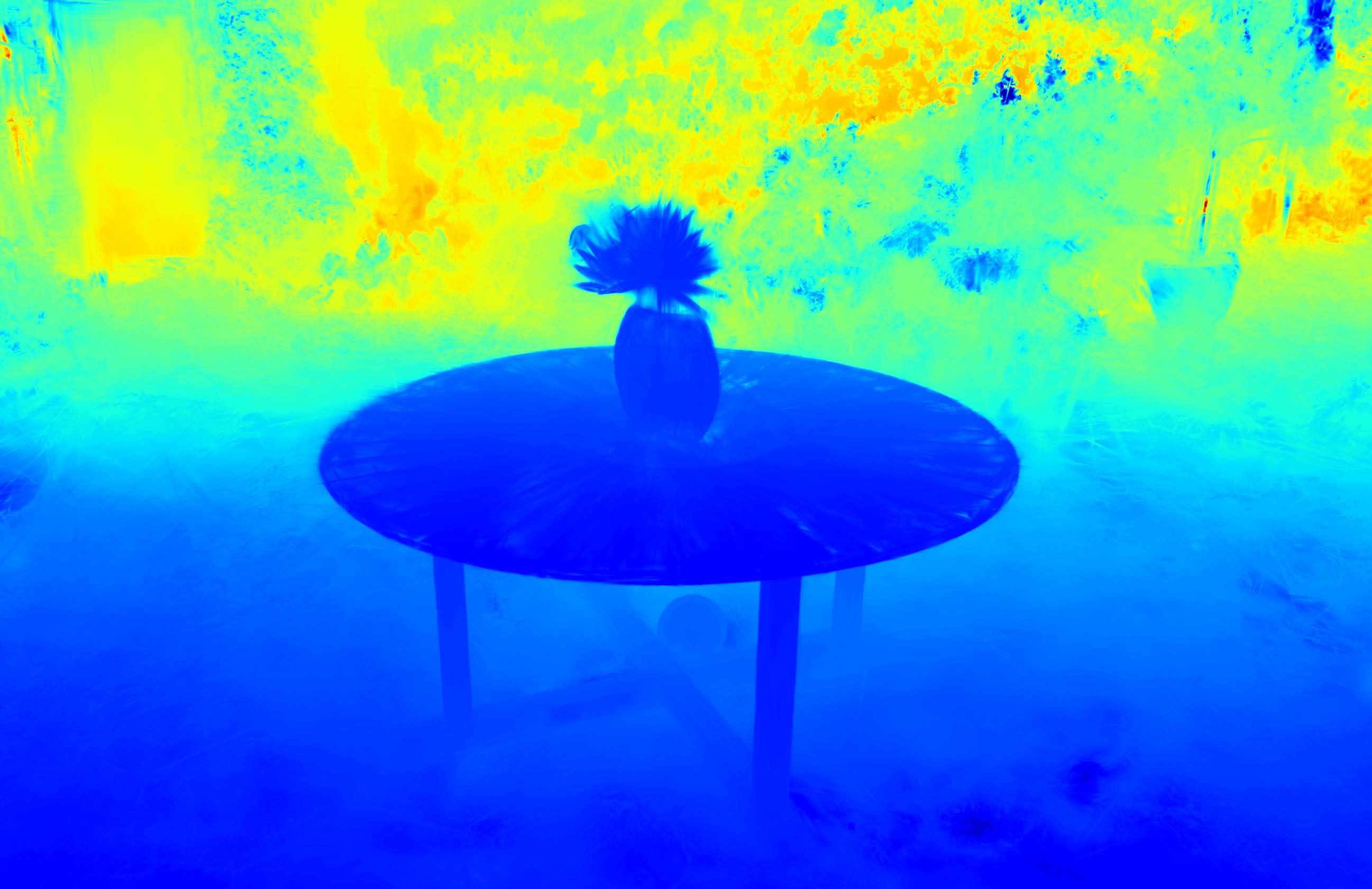
(c)

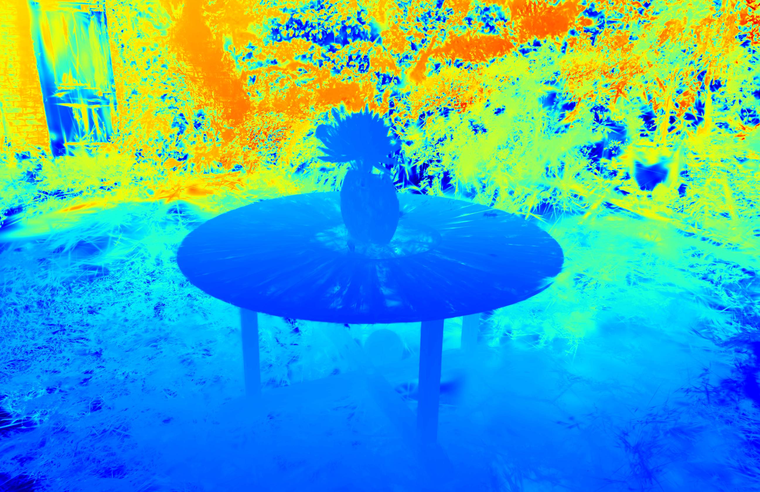
(d)

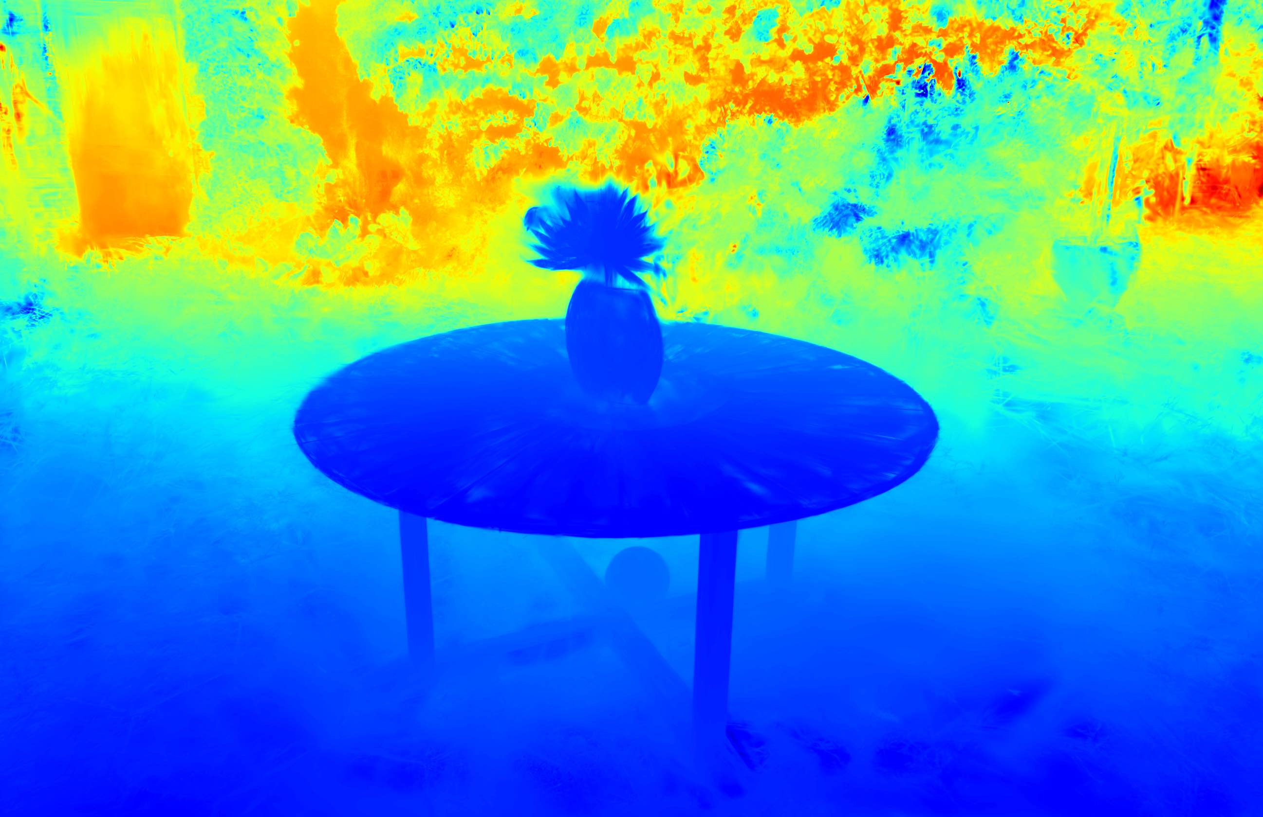
(e)

Figure 6: Our full model performs best in terms of image renders and depth maps. Our full model combines the best of different subcomponents to generate high-quality depth maps (e.g. it retains the smoothness of the depth correlation loss while learning background details from floater pruning and diffusion). For depth maps, the ground truth is the output of the Monodepth model as we do not have the true ground truth depth.

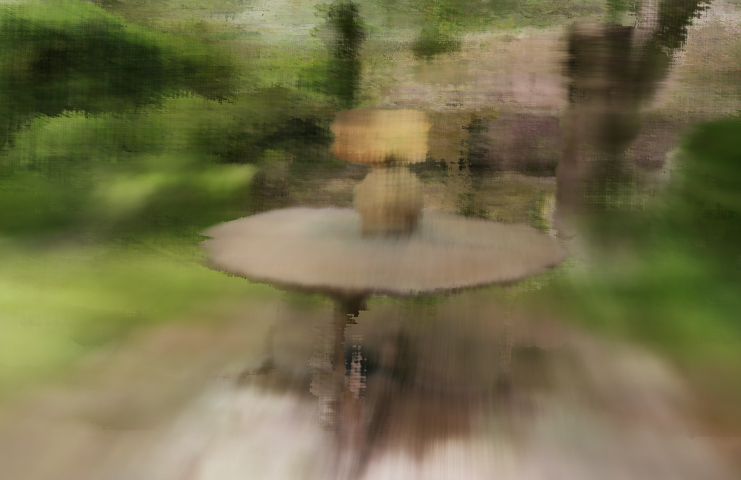
(a)

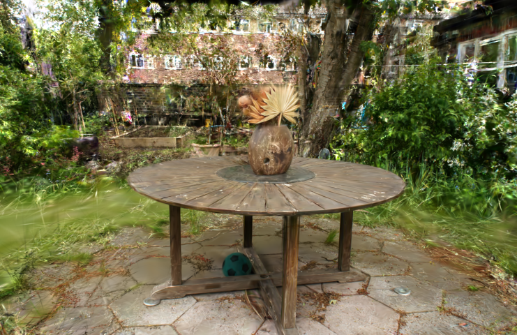
(b)

Figure 7: NeRF and 3DGS and suffer from different failure modes. NeRF and 3DGS have different failure modes. NeRF tends to oversmooth ambiguous areas of the scene, while 3DGS spawns many gaussians leading to high frequency artifacts.

Model	PSNR $\uparrow$	SSIM $\uparrow$	LPIPS $\downarrow$
w/o Floater Pruning	15.7264	0.3785	0.5004
w/o Correlation Loss	16.1335	0.3635	0.5041
w/o Diffusion Loss	16.7385	0.4009	0.4979
Full Model	16.8535	0.4055	0.4953

Table 3: An ablation study on the garden scene shows our full model performs best. Each component individually provides benefits that combine to enable the performance of our full model. The best result is bolded and the second best is underlined.

We additionally run ablation studies to examine the effects of each of the individual components we introduce. Specifically, we ablate the depth correlation loss, the score distillation sampling loss, and floater pruning. Results are shown in Tab. 3 and in Fig. 6. As can be seen in Tab. 3, our full model performs best on all three metrics, and our novel floater pruning operator provides the most benefit among the three components of our technique (drop of  1 PSNR when removing it). Additionally, Fig. 6 highlights the benefits of the depth correlation loss, particularly for the depth maps. Without the depth correlation loss, there are many discontinuities and sharp features in the depth map, likely because there is very little regularization and the model is trying to learn to represent all training views.

Implementation Details

Our training procedure is built on top of the procedure introduced in 3D Gaussian Splatting [11]. We train for 30k iterations with learning rates for the gaussian represetation components taken from [11]. We apply the depth correlation loss every iteration with a patch size of 128 pixels and select 50% of all patches per iteration. We apply the diffusion loss randomly for 20% of iterations during the last 10k steps. We randomize angles from -10° to +10° around the scene center. We additionally apply our floater pruning technique at 20k and 25k iterations with $a=97$ and $b=-8$. We choose $\lambda_{depth}=0.1$ and $\lambda_{SDS}=5\times 10^{-4}$.

5 Conclusion

Limitations

One key limitation of our method is that because it is built on top of 3D Gaussian Splatting, it is heavily reliant on the initial point cloud provided by COLMAP. If this point cloud is inaccurate or lacks detail, our model may struggle to compensate adequately, leading to under-reconstructions, especially in areas distant from the scene center. This limitation is especially prominent in the sparse view setting, as our initial training views lack substantial coverage. As a result, the input point clouds are relatively small, with many tested scenes being initialized with fewer than 20 points in total. To address this challenge, future efforts could involve investigating point cloud densification techniques as data augmentations.

In this paper, we introduce a novel 3D gaussian splatting based technique for few-shot novel view synthesis. We leverage the explicit nature of the 3D gaussian representation to introduce a novel pruning operator designed to reduce and remove ”floater” artifacts. Applied to the Mip-NeRF 360 dataset, we show our technique can achieve state-of-the-art performance on few shot novel view synthesis for 360° unbounded scenes.

Supplementary Material

Supplementary Contents

This supplementary is organized as follows:

• Section A shows quantitative comparisons against more baselines on the Mip-NeRF 360 dataset.

• Section B provides comparisons on forward facing scenes from the DTU dataset.

• Section C provides more qualitative comparisons between our method and baselines.

• Section D provides code snippets for some of our key components.

A More Comparisons on Mip-NeRF 360 Dataset

In this section, we expand upon the results in the main paper and compare against additional baselines on the Mip-NeRF 360 dataset [2]. We compare against RegNeRF [20] and ViP-NeRF [29], both of which are techniques for few-shot view synthesis using NeRFs.

Model	PSNR $\uparrow$	SSIM $\uparrow$	LPIPS $\downarrow$	Runtime (h)	Render FPS
SparseNeRF	11.5638	0.3206	0.6984	4	1/120
Base 3DGS	15.3840	0.4415	0.5061	0.5	30
Mip-NeRF 360	17.1044	0.4660	0.5750	3	1/120
RegNeRF	11.7379	0.2266	0.6892	4	1/120
ViP-NeRF	11.1622	0.2291	0.7132	4	1/120
Ours	16.6898	0.4899	0.4849	0.75	30

Table D: Additional sparse-view NeRF baselines. Runtimes are recorded on 1 RTX3090.

We out-perform both new models RegNeRF [20] and ViP-NeRF [29] on PSNR, SSIM and LPIPS while also being significantly faster for both training and inference.

B Comparisons on Frontal Scenes from DTU Dataset

In this section, we provide comparisons on forward-facing scenes from the DTU dataset [10]. Although our technique is designed for unbounded 360° scenes, we provide these comparisons because a large set of prior work on the task of few-shot novel view synthesis has been focused on the forward-facing setting.

Model	PSNR			SSIM			LPIPS
	scan40	scan63	scan144	scan40	scan63	scan144	scan40	scan63	scan144
Original 3DGS	15.4527	13.8022	18.3623	0.5988	0.8025	0.6990	0.3095	0.1722	0.2159
RegNeRF	18.8625	22.6440	21.0046	0.6437	0.9268	0.8248	0.2277	0.0599	0.1503
Ours	19.0773	20.6502	18.2723	0.6319	0.8594	0.7295	0.2792	0.1131	0.2000

Table E: Additional results on the forward-facing DTU dataset. This is a selected quantitative analysis

We perform comparably on the DTU dataset, with a significant boost to base 3DGS. RegNeRF was chosen because of its available pretrained models.

C More Qualitative Results

In this section, we provide additional qualitative results from our method. These examples are taken from the Mip-NeRF 360 datasets. The results are shown in Fig. A.

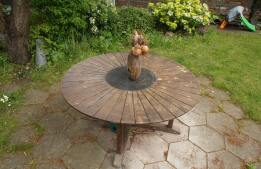
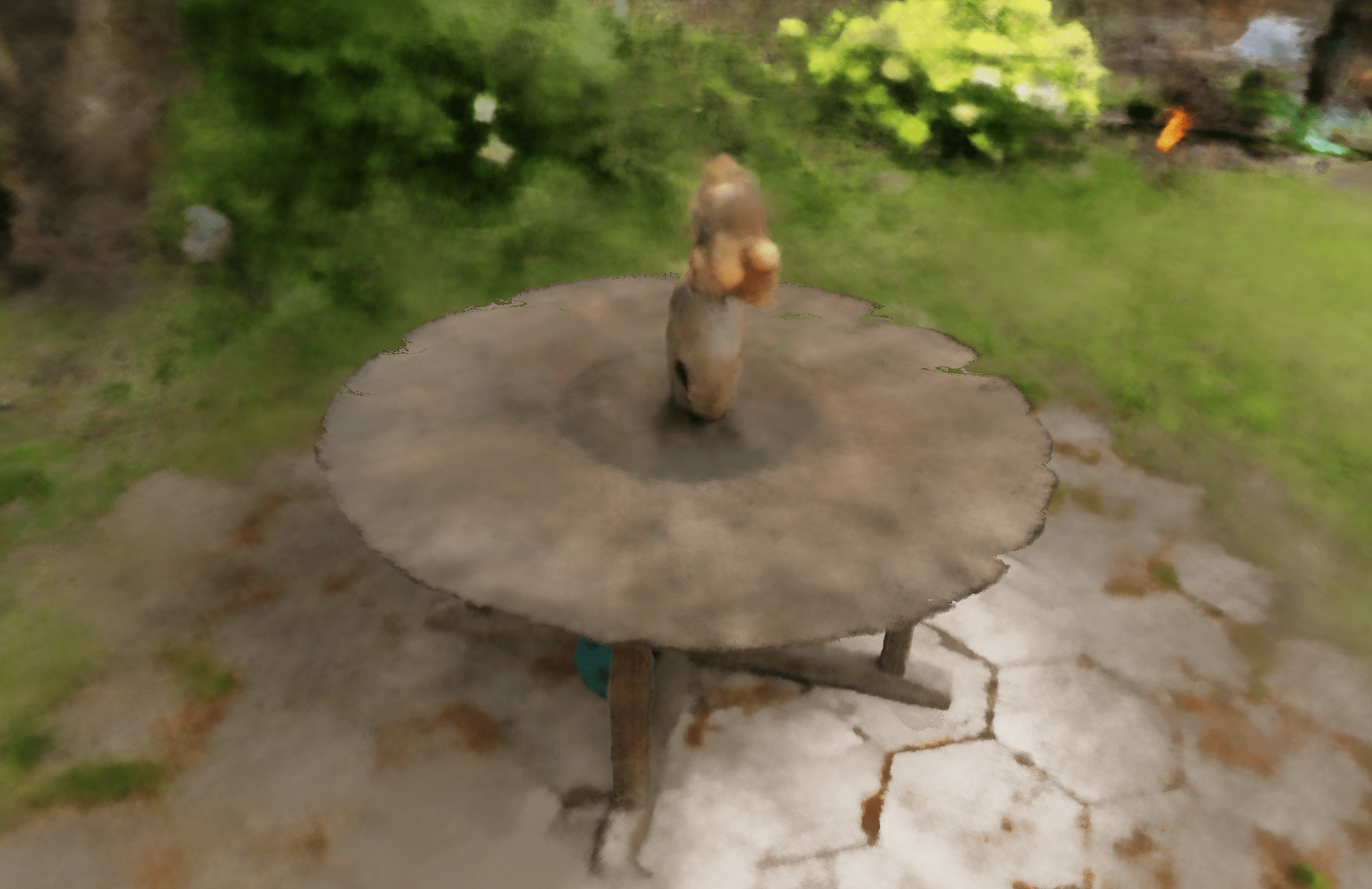
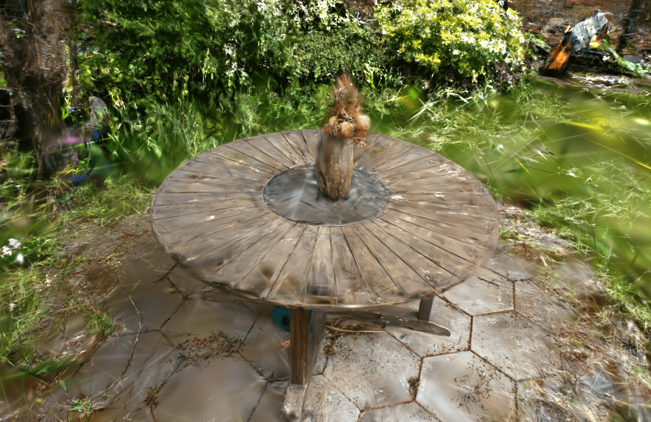
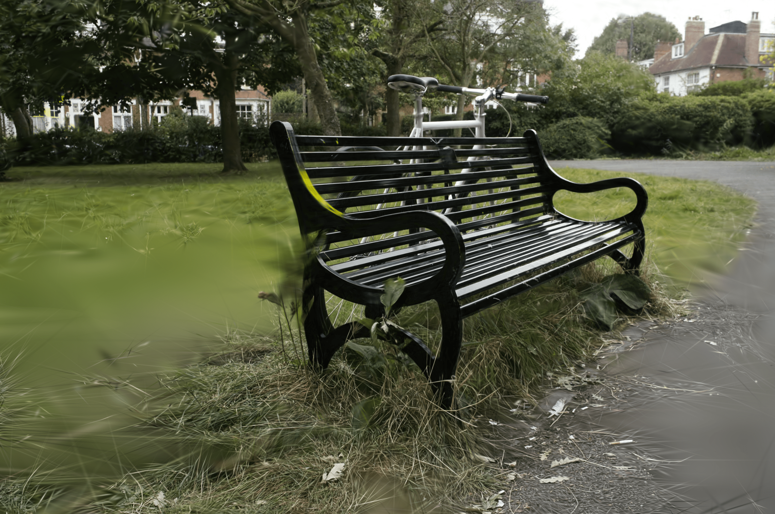
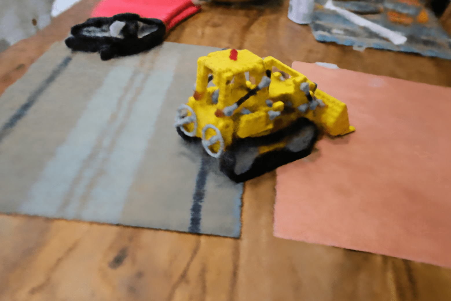
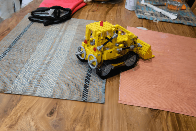
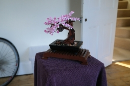
(a)

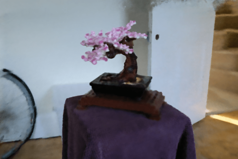
(b)

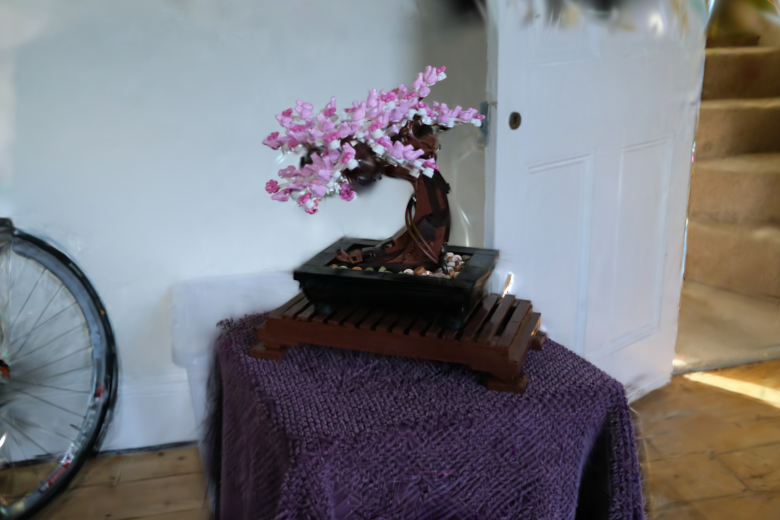
(c)

Figure A: Qualitative comparisons between our method and Mip-NeRF 360 on the Mip-NeRF 360 dataset. Our method produces sharper results on novel views.

D Code Snippets

In this section, we provide code snippets for key parts of our method. In specific, we provide code snippets for the depth ranking loss and the floater removal. Fuller versions of our method are provided in as code files in the supplementary material. All code is written in Python with PyTorch.

Ranking Loss

:

⬇

1def local_pearson_loss(depth_src, depth_target, box_p, p_corr):

2 # Randomly select patch, top left corner of the patch (x_0,y_0) has to be 0 <= x_0 <= max_h, 0 <= y_0 <= max_w

3 num_box_h = math.floor(depth_src.shape[0]/box_p)

4 num_box_w = math.floor(depth_src.shape[1]/box_p)

5 max_h = depth_src.shape[0] - box_p

6 max_w = depth_src.shape[1] - box_p

7 _loss = torch.tensor(0.0,device=’cuda’)

8 # Select the number of boxes based on hyperparameter p_corr

9 n_corr = int(p_corr * num_box_h * num_box_w)

10 x_0 = torch.randint(0, max_h, size=(n_corr,), device = ’cuda’)

11 y_0 = torch.randint(0, max_w, size=(n_corr,), device = ’cuda’)

12 x_1 = x_0 + box_p

13 y_1 = y_0 + box_p

14 _loss = torch.tensor(0.0,device=’cuda’)

15 for i in range(len(x_0)):

16 _loss += pearson_depth_loss(depth_src[x_0[i]:x_1[i],y_0[i]:y_1[i]].reshape(-1), depth_target[x_0[i]:x_1[i],y_0[i]:y_1[i]].reshape(-1))

17 return _loss/n_corr

Floater Removal

:

⬇

1def prune_floaters(viewpoint_stack, gaussians, pipe, background, dataset, iteration):

2 N = #number of gaussians

3 mask = #initialize gaussian pruning masks

4

5

6 dips = [] #dip statistic

7 point_lists = [] #depth-ordered gaussian IDs

8 means2Ds = [] #view-space means

9 conic_opacities = [] #covariance matrix and opacity neatly packed

10 mode_ids = [] #our mode gaussians

11 diffs = [] #relative differences

12 names = [] #image names

13

14 for view in viewpoint_stack: #iterate over views

15 names.append(view.image_name)

16 render_pkg = render(.)

17 mode_id, mode, point_list, depth, means2D, conic_opacity = #extract from renders

18 diff = calc_diff(mode, depth)

19 means2Ds.append(means2D)

20 conic_opacities.append(conic_opacity)

21 mode_ids.append(mode_id)

22 diffs.append(diff)

23 dips.append(diptest.dipstat(diff[diff > 0].cpu().numpy()))

24

25 dips = np.array(dips)

26 avg_dip = dips.mean()

27 perc = 97*np.exp(-8*avg_dip) #empirically calculated curve

28

29 for name, mode_id, point_list, diff, means2D, conic_opacity in zip(names, mode_ids, point_lists, diffs, means2Ds, conic_opacities):

30 submask = #initialize mask for current view

31

32 diffpos = diff[diff > 0] #positive differences

33 threshold = np.percentile(diffpos, perc)

34 pruned_modes_mask = (diff > threshold)

35

36 #get pixel indices of mode mask

37 pixel_y, pixel_x = torch.meshgrid(torch.arange(pruned_modes_mask.shape[0]), torch.arange(pruned_modes_mask.shape[1]), indexing=’ij’)

38 prune_mode_ids = mode_id[:,pruned_modes_mask]

39 pixel_x = pixel_x[pruned_modes_mask]

40 pixel_y = pixel_y[pruned_modes_mask]

41

42 #filter out unpopulated modes

43 neg_mask = (prune_mode_ids == -1).any(dim=0)

44 prune_mode_ids = prune_mode_ids[:,~neg_mask]

45 pixel_x = pixel_x[~neg_mask]

46 pixel_y = pixel_y[~neg_mask]

47

48 #aggregate unique gaussians over selected mode ranges

49 selected_gaussians = set()

50 for j in range(prune_mode_ids.shape[-1]):

51 x = pixel_x[j]

52 y = pixel_y[j]

53 gausses = point_list[prune_mode_ids[0,j]:prune_mode_ids[1,j]+1].long()

54 c_opacs = conic_opacity[gausses]

55 m2Ds = means2D[gausses]

56

57 #test whether we are within sufficient gaussian range

58 test_alpha = calc_alpha(m2Ds, c_opacs, x, y)

59 alpha_mask = test_alpha > dataset.power_thresh

60 gausses = gausses[alpha_mask]

61

62 selected_gaussians.update(gausses.tolist())

63

64 submask[list(selected_gaussians)] = True

65

66 #aggregate mask

67 mask = mask | submask

68

69 num_points_pruned = submask.sum()

70 print(f’Pruning␣{num_points_pruned}␣gaussians’)

71

72 gaussians.prune_points(mask)

References

- Barron et al. [2021] Jonathan T. Barron, Ben Mildenhall, Matthew Tancik, Peter Hedman, Ricardo Martin-Brualla, and Pratul P. Srinivasan. Mip-nerf: A multiscale representation for anti-aliasing neural radiance fields. ICCV, 2021.
- Barron et al. [2022] Jonathan T. Barron, Ben Mildenhall, Dor Verbin, Pratul P. Srinivasan, and Peter Hedman. Mip-nerf 360: Unbounded anti-aliased neural radiance fields. CVPR, 2022.
- Deng et al. [2022] Kangle Deng, Andrew Liu, Jun-Yan Zhu, and Deva Ramanan. Depth-supervised NeRF: Fewer views and faster training for free. In Proceedings of the IEEE/CVF Conference on Computer Vision and Pattern Recognition (CVPR), 2022.
- Hartigan and Hartigan [1985] J. A. Hartigan and P. M. Hartigan. The Dip Test of Unimodality. The Annals of Statistics, 13(1):70 – 84, 1985.
- Ho et al. [2020] Jonathan Ho, Ajay Jain, and Pieter Abbeel. Denoising diffusion probabilistic models. Advances in neural information processing systems, 33:6840–6851, 2020.
- Hong et al. [2023] Yicong Hong, Kai Zhang, Jiuxiang Gu, Sai Bi, Yang Zhou, Difan Liu, Feng Liu, Kalyan Sunkavalli, Trung Bui, and Hao Tan. Lrm: Large reconstruction model for single image to 3d. arXiv preprint arXiv:2311.04400, 2023.
- Irshad et al. [2023] Muhammad Zubair Irshad, Sergey Zakharov, Katherine Liu, Vitor Guizilini, Thomas Kollar, Adrien Gaidon, Zsolt Kira, and Rares Ambrus. Neo 360: Neural fields for sparse view synthesis of outdoor scenes. In Proceedings of the IEEE/CVF International Conference on Computer Vision, pages 9187–9198, 2023.
- Jain et al. [2021] Ajay Jain, Matthew Tancik, and Pieter Abbeel. Putting nerf on a diet: Semantically consistent few-shot view synthesis. In Proceedings of the IEEE/CVF International Conference on Computer Vision (ICCV), pages 5885–5894, 2021.
- Jain et al. [2022] Ajay Jain, Ben Mildenhall, Jonathan T. Barron, Pieter Abbeel, and Ben Poole. Zero-shot text-guided object generation with dream fields. 2022.
- Jensen et al. [2014] Rasmus Jensen, Anders Dahl, George Vogiatzis, Engil Tola, and Henrik Aanæs. Large scale multi-view stereopsis evaluation. In 2014 IEEE Conference on Computer Vision and Pattern Recognition, pages 406–413. IEEE, 2014.
- Kerbl et al. [2023] Bernhard Kerbl, Georgios Kopanas, Thomas Leimkühler, and George Drettakis. 3d gaussian splatting for real-time radiance field rendering. ACM Transactions on Graphics, 42(4), 2023.
- Levis et al. [2022] Aviad Levis, Pratul P Srinivasan, Andrew A Chael, Ren Ng, and Katherine L Bouman. Gravitationally lensed black hole emission tomography. In Proceedings of the IEEE/CVF Conference on Computer Vision and Pattern Recognition, pages 19841–19850, 2022.
- Liu et al. [2023a] Minghua Liu, Chao Xu, Haian Jin, Linghao Chen, Zexiang Xu, Hao Su, et al. One-2-3-45: Any single image to 3d mesh in 45 seconds without per-shape optimization. arXiv preprint arXiv:2306.16928, 2023a.
- Liu et al. [2023b] Ruoshi Liu, Rundi Wu, Basile Van Hoorick, Pavel Tokmakov, Sergey Zakharov, and Carl Vondrick. Zero-1-to-3: Zero-shot one image to 3d object, 2023b.
- Luiten et al. [2023] Jonathon Luiten, Georgios Kopanas, Bastian Leibe, and Deva Ramanan. Dynamic 3d gaussians: Tracking by persistent dynamic view synthesis. arXiv preprint arXiv:2308.09713, 2023.
- Miangoleh et al. [2021] S. Mahdi H. Miangoleh, Sebastian Dille, Long Mai, Sylvain Paris, and Yağız Aksoy. Boosting monocular depth estimation models to high-resolution via content-adaptive multi-resolution merging. In Proc. CVPR, 2021.
- Mildenhall et al. [2020] Ben Mildenhall, Pratul P. Srinivasan, Matthew Tancik, Jonathan T. Barron, Ravi Ramamoorthi, and Ren Ng. Nerf: Representing scenes as neural radiance fields for view synthesis. In ECCV, 2020.
- Mildenhall et al. [2022] Ben Mildenhall, Peter Hedman, Ricardo Martin-Brualla, Pratul P. Srinivasan, and Jonathan T. Barron. NeRF in the dark: High dynamic range view synthesis from noisy raw images. CVPR, 2022.
- Müller et al. [2022] Thomas Müller, Alex Evans, Christoph Schied, and Alexander Keller. Instant neural graphics primitives with a multiresolution hash encoding. ACM Trans. Graph., 41(4):102:1–102:15, 2022.
- Niemeyer et al. [2022] Michael Niemeyer, Jonathan T. Barron, Ben Mildenhall, Mehdi S. M. Sajjadi, Andreas Geiger, and Noha Radwan. Regnerf: Regularizing neural radiance fields for view synthesis from sparse inputs. In Proc. IEEE Conf. on Computer Vision and Pattern Recognition (CVPR), 2022.
- Po et al. [2023] Ryan Po, Wang Yifan, Vladislav Golyanik, Kfir Aberman, Jonathan T Barron, Amit H Bermano, Eric Ryan Chan, Tali Dekel, Aleksander Holynski, Angjoo Kanazawa, et al. State of the art on diffusion models for visual computing. arXiv preprint arXiv:2310.07204, 2023.
- Poole et al. [2022] Ben Poole, Ajay Jain, Jonathan T Barron, and Ben Mildenhall. Dreamfusion: Text-to-3d using 2d diffusion. arXiv preprint arXiv:2209.14988, 2022.
- Ranftl et al. [2020] René Ranftl, Katrin Lasinger, David Hafner, Konrad Schindler, and Vladlen Koltun. Towards robust monocular depth estimation: Mixing datasets for zero-shot cross-dataset transfer. IEEE Transactions on Pattern Analysis and Machine Intelligence (TPAMI), 2020.
- Ranftl et al. [2021] René Ranftl, Alexey Bochkovskiy, and Vladlen Koltun. Vision transformers for dense prediction. ArXiv preprint, 2021.
- Rodrigues [1840] O. Rodrigues. Lois du mouvement des systèmes de points matériels. Journal de l’Ecole Royale Polytechnique, 19:319–429, 1840.
- Rombach et al. [2022] Robin Rombach, Andreas Blattmann, Dominik Lorenz, Patrick Esser, and Björn Ommer. High-resolution image synthesis with latent diffusion models. In Proceedings of the IEEE/CVF conference on computer vision and pattern recognition, pages 10684–10695, 2022.
- Schönberger and Frahm [2016] Johannes Lutz Schönberger and Jan-Michael Frahm. Structure-from-motion revisited. In Conference on Computer Vision and Pattern Recognition (CVPR), 2016.
- Schönberger et al. [2016] Johannes Lutz Schönberger, Enliang Zheng, Marc Pollefeys, and Jan-Michael Frahm. Pixelwise view selection for unstructured multi-view stereo. In European Conference on Computer Vision (ECCV), 2016.
- Somraj and Soundararajan [2023] Nagabhushan Somraj and Rajiv Soundararajan. Vip-nerf: Visibility prior for sparse input neural radiance fields. 2023.
- Srinivasan et al. [2019] Pratul P. Srinivasan, Richard Tucker, Jonathan T. Barron, Ravi Ramamoorthi, Ren Ng, and Noah Snavely. Pushing the boundaries of view extrapolation with multiplane images. CVPR, 2019.
- Stan et al. [2023] Gabriela Ben Melech Stan, Diana Wofk, Scottie Fox, Alex Redden, Will Saxton, Jean Yu, Estelle Aflalo, Shao-Yen Tseng, Fabio Nonato, Matthias Muller, et al. Ldm3d: Latent diffusion model for 3d. arXiv preprint arXiv:2305.10853, 2023.
- Sun et al. [2018] Xingyuan Sun, Jiajun Wu, Xiuming Zhang, Zhoutong Zhang, Chengkai Zhang, Tianfan Xue, Joshua B Tenenbaum, and William T Freeman. Pix3d: Dataset and methods for single-image 3d shape modeling. In IEEE Conference on Computer Vision and Pattern Recognition (CVPR), 2018.
- Tancik et al. [2020] Matthew Tancik, Pratul Srinivasan, Ben Mildenhall, Sara Fridovich-Keil, Nithin Raghavan, Utkarsh Singhal, Ravi Ramamoorthi, Jonathan Barron, and Ren Ng. Fourier features let networks learn high frequency functions in low dimensional domains. Advances in Neural Information Processing Systems, 33:7537–7547, 2020.
- Tang et al. [2023] Jiaxiang Tang, Jiawei Ren, Hang Zhou, Ziwei Liu, and Gang Zeng. Dreamgaussian: Generative gaussian splatting for efficient 3d content creation. arXiv preprint arXiv:2309.16653, 2023.
- Tucker and Snavely [2020] Richard Tucker and Noah Snavely. Single-view view synthesis with multiplane images. In Proceedings of the IEEE/CVF Conference on Computer Vision and Pattern Recognition, pages 551–560, 2020.
- Wang et al. [2023] Guangcong Wang, Zhaoxi Chen, Chen Change Loy, and Ziwei Liu. Sparsenerf: Distilling depth ranking for few-shot novel view synthesis. IEEE/CVF International Conference on Computer Vision (ICCV), 2023.
- Wang et al. [2004] Zhou Wang, A.C. Bovik, H.R. Sheikh, and E.P. Simoncelli. Image quality assessment: from error visibility to structural similarity. IEEE Transactions on Image Processing, 13(4):600–612, 2004.
- Weng et al. [2022] Chung-Yi Weng, Brian Curless, Pratul P. Srinivasan, Jonathan T. Barron, and Ira Kemelmacher-Shlizerman. HumanNeRF: Free-viewpoint rendering of moving people from monocular video. In Proceedings of the IEEE/CVF Conference on Computer Vision and Pattern Recognition (CVPR), pages 16210–16220, 2022.
- Wu et al. [2023] Guanjun Wu, Taoran Yi, Jiemin Fang, Lingxi Xie, Xiaopeng Zhang, Wei Wei, Wenyu Liu, Qi Tian, and Xinggang Wang. 4d gaussian splatting for real-time dynamic scene rendering. arXiv preprint arXiv:2310.08528, 2023.
- Xu et al. [2022] Dejia Xu, Yifan Jiang, Peihao Wang, Zhiwen Fan, Yi Wang, and Zhangyang Wang. Neurallift-360: Lifting an in-the-wild 2d photo to a 3d object with 360° views. 2022.
- Yi et al. [2023] Taoran Yi, Jiemin Fang, Guanjun Wu, Lingxi Xie, Xiaopeng Zhang, Wenyu Liu, Qi Tian, and Xinggang Wang. Gaussiandreamer: Fast generation from text to 3d gaussian splatting with point cloud priors. arXiv preprint arXiv:2310.08529, 2023.
- Zhang et al. [2021] Xiuming Zhang, Pratul P Srinivasan, Boyang Deng, Paul Debevec, William T Freeman, and Jonathan T Barron. Nerfactor: Neural factorization of shape and reflectance under an unknown illumination. ACM Transactions on Graphics (ToG), 40(6):1–18, 2021.
- Zhou et al. [2018] Tinghui Zhou, Richard Tucker, John Flynn, Graham Fyffe, and Noah Snavely. Stereo magnification: Learning view synthesis using multiplane images. arXiv preprint arXiv:1805.09817, 2018.
- Zielonka et al. [2023] Wojciech Zielonka, Timur Bagautdinov, Shunsuke Saito, Michael Zollhöfer, Justus Thies, and Javier Romero. Drivable 3d gaussian avatars. arXiv preprint arXiv:2311.08581, 2023.
- Zwicker et al. [2001a] M. Zwicker, H. Pfister, J. van Baar, and M. Gross. Ewa volume splatting. In Proceedings Visualization, 2001. VIS ’01., pages 29–538, 2001a.
- Zwicker et al. [2001b] Matthias Zwicker, Hanspeter Pfister, Jeroen Van Baar, and Markus Gross. Surface splatting. In Proceedings of the 28th annual conference on Computer graphics and interactive techniques, pages 371–378, 2001b.