Scalable Bayesian uncertainty quantification with data-driven priors for radio interferometric imaging

Abstract

Next-generation radio interferometers like the Square Kilometer Array have the potential to unlock scientific discoveries thanks to their unprecedented angular resolution and sensitivity. One key to unlocking their potential resides in handling the deluge and complexity of incoming data. This challenge requires building radio interferometric imaging methods that can cope with the massive data sizes and provide high-quality image reconstructions with uncertainty quantification (UQ). This work proposes a method coined QuantifAI to address UQ in radio-interferometric imaging with data-driven (learned) priors for high-dimensional settings. Our model, rooted in the Bayesian framework, uses a physically motivated model for the likelihood. The model exploits a data-driven convex prior, which can encode complex information learned implicitly from simulations and guarantee the log-concavity of the posterior. We leverage probability concentration phenomena of high-dimensional log-concave posteriors that let us obtain information about the posterior, avoiding MCMC sampling techniques. We rely on convex optimisation methods to compute the MAP estimation, which is known to be faster and better scale with dimension than MCMC sampling strategies. Our method allows us to compute local credible intervals, i.e., Bayesian error bars, and perform hypothesis testing of structure on the reconstructed image. In addition, we propose a novel blazing-fast method to compute pixel-wise uncertainties at different scales. We demonstrate our method by reconstructing radio-interferometric images in a simulated setting and carrying out fast and scalable UQ, which we validate with MCMC sampling. Our method shows an improved image quality and more meaningful uncertainties than the benchmark method based on a sparsity-promoting prior. QuantifAI’s source code and scripts for the numerical experiment of this paper are available from github.com/astro-informatics/QuantifAI.

1 Introduction

Radio astronomy plays a crucial role in expanding our understanding of the Universe, offering a unique perspective on astrophysical and cosmological phenomena. Among the transformative tools in an astronomer’s toolkit, radio interferometric (RI) imaging stands out as an indispensable technique. Aperture synthesis and radio interferometry (Thompson et al., 2017) allow us to achieve high angular resolutions providing immense power to resolve objects. Furthermore, radio frequency signals are only weakly attenuated by our atmosphere, allowing for observations at the Earth’s surface. The unparalleled angular resolution, high sensitivity and the different phenomena emitting in the radio wavelength regime make RI an ideal candidate to reshape our understanding of the Universe and push the boundaries of science.

The advent of the Square Kilometre Array (SKA, Dewdney et al., 2009) heralds a new era in radio astronomy (Braun et al., 2015) spanning the study from the epoch of reionisation and fast radio bursts to galaxy evolution and dark energy. SKA’s vast collecting area and sensitivity promise to revolutionise our observational capabilities, opening doors to discoveries we can barely imagine today. However, this transformative potential comes with the formidable computational challenge of processing and making sense of the unprecedented volume of SKA-generated data. Developing and implementing algorithms that can efficiently handle SKA’s data deluge is a challenge. In addition, achieving the high reconstruction performance required to unlock SKA’s full potential is a significant obstacle in the SKA’s data processing requirements.

The aperture synthesis techniques in RI probe the sky by acquiring specific Fourier measurements, which results in incomplete coverage of the Fourier domain of the sky’s image of interest. Adding observational noise to the incomplete Fourier coverage makes the problem of estimating the underlying sky image an ill-posed inverse problem, which we know as RI imaging. Having a way to quantify the uncertainty in the image reconstructions becomes essential given the uncertainties involved in the RI imaging problem. To make scientifically sound inferences and informed decisions, we need the ability to quantify these uncertainties rigorously. This motivates the development of uncertainty quantification (UQ) methods tailored to the complexities of radio interferometric data, where scalability and performance play a central role. We need to ensure that our reconstructions are not only insightful but also trustworthy.

In a nutshell, we are in the quest for RI imaging methods that can deliver precision with uncertainty quantification and that are highly scalable. Existing methods only tackle some of these three requirements. The widely used CLEAN algorithm (Högbom, 1974) built its success on scalability and fast inference. CLEAN and its extensions (Cornwell, 2008; Offringa et al., 2014; Offringa & Smirnov, 2017) have been continuously used in many RI imaging pipelines since its inception. Despite offering limited imaging quality and reconstruction artefacts compared to other approaches, CLEAN stands out due to its scalability. More recent approaches leverage compressed sensing theory, relying on sparse priors (often in wavelet representations) and convex optimisation techniques (Wiaux et al., 2009; McEwen & Wiaux, 2011; Carrillo et al., 2012, 2014; Dabbech, A. et al., 2015; Dabbech et al., 2018; Pratley et al., 2017). These methods have been shown to improve the reconstruction quality at the expense of increased computational complexity. Considerable work has been directed to parallelisation and acceleration efforts for sparsity-based methods (Onose et al., 2016; Pratley et al., 2019b, a; Thouvenin et al., 2022a, b).

The deep learning revolution has introduced a powerful way to encode complex image priors in neural networks, which may be used to solve complex high-dimensional inverse problems. This data-driven or learned paradigm has gained a lot of traction across imaging landscape problems, including RI imaging (Allam, 2016; Terris et al., 2022; Aghabiglou et al., 2023; Mars et al., 2023b). Learned methods can improve the reconstruction quality with respect to handcrafted priors, such as sparsity-based wavelet priors, as well as provide acceleration (Terris et al., 2022; Mars et al., 2023b, a) to convex optimisation-based methods.

Unfortunately, none of the RI imaging methods mentioned, learned, sparsity-based or CLEAN-based, provide UQ tools. Cai et al. (2018a, b) proposed methods for UQ on RI imaging problems. Cai et al. (2018a) leverages proximal MCMC methods (Pereyra, 2016) to provide support for sparsity-promoting priors. The proposed method allows them to reconstruct the image and provide UQ by sampling the posterior probability distribution. The drawback of the method is the high computational cost suffered by all MCMC sampling techniques. The companion paper, Cai et al. (2018b), overcomes the need for posterior sampling with maximum-a-posteriori (MAP) based UQ (Pereyra, 2017) relying on convex optimisation techniques. The new method (Cai et al., 2018b) provides a significant speed-up with respect to the sampling-based method (Cai et al., 2018a), but its reconstruction quality is limited to sparsity-promoting priors.

In this article, we delve into the forefront of RI imaging and propose a method coined QuantifAI, based on data-driven priors, capable of delivering high-quality reconstructions with uncertainty quantification and being highly scalable. The method relies on the mathematically principled Bayesian framework to provide an understanding of the uncertainties through the posterior distribution. By restricting our model to log-concave posteriors we can exploit recent MAP-based UQ techniques (Pereyra, 2017), providing scalable optimisation-based UQ. We build upon recent advances in neural-network-based convex regularisers (Goujon et al., 2023b), allowing us to obtain state-of-the-art reconstruction quality and more meaningful uncertainties. On top of the hypothesis tests of structure on the reconstructed image, we propose a blazing-fast method to estimate pixel-wise uncertainties as a function of scale.

The remainder of this article is organised as follows. In Section 2, we start by reviewing the RI imaging and techniques for the resulting inverse problem. Section 3 describes QuantifAI, the proposed method, and the RI image reconstruction algorithm. In Section 4, we introduce the core of our scalable UQ and the different UQ techniques it allows. The experimental results, including the performance of QuantifAI reconstruction and its UQ techniques, are presented in Section 5. We provide concluding remarks and present some future perspectives in Section 6.

2 Radio interferometric imaging

In this section, we start by reviewing the RI imaging inverse problem and discuss approaches to tackle it, including sparsity-based regularisation, the CLEAN method, and learned approaches. We then introduce the Bayesian framework elements needed such as MAP estimation and proximal MCMC sampling algorithms that will be later used as validation.

2.1 Radio interferometry

The interferometric measurement equation for a radio telescope (Thompson et al., 2017) in the monochromatic setting relates our observations represented by the visibility function $\mathcal{Y}$ to the sky brightness $\mathcal{X}$, which we want to reconstruct,

$$\mathcal{Y}( u,v,w)=\iint\frac{\mathcal{X}(l,m)\,\mathcal{A}(l,m)}{\sqrt{1-l^{2}-m^{2}}}$$ (1)

$$\times\exp\left[-2\pi\text{i}w\left(\sqrt{1-l^{2}-m^{2}}-1\right)\right]\exp\left[-2\pi\text{i}\left(lu+mv\right)\right]\text{d}l\text{d}m\,,$$

where $\mathbf{u}=(u,v,w)$ are the interferometer baseline coordinates with units depending on the observation wavelength, $\mathbf{l}=(l,m,n)$ are cosine sky coordinates restricted to the unit sphere, and $\mathcal{A}$ includes direction-dependent effects (DDEs) like the primary beam of the dishes. The previous general model allows us to consider different DDEs through $\mathcal{A}$ and non-coplanar effects through the exponential term in $w$. These effects become considerable when considering wide fields of view and long baselines. There exists a rich body of literature incorporating such effects, e.g., Smirnov, O. M. (2011a, b, c, d); Thompson et al. (2017), and there are scalable algorithms that take them into account, e.g., Pratley et al. (2019b).

In this article, for the sake of simplicity but without loss of generality, we assume the coplanar setting, where the antennas are located in the same $w$ plane. We also assume that we observe a small field of view such that $1-l^{2}-m^{2}\approx 1$. Consequently, we have $\exp\left[-2\pi\text{i}w\left(\sqrt{1-l^{2}-m^{2}}-1\right)\right]\approx 1$, and Equation 1 reduces to

$$\mathcal{Y}(u,v)\approx\iint\mathcal{X}(l,m)\,\mathcal{A}(l,m)\exp\left[-2\pi\text{i}\left(lu+mv\right)\right]\text{d}l\text{d}m\,.$$ (2)

From the previous equation, we can notice the remarkable result of $\mathcal{Y}(u,v)=\mathcal{F}(\mathcal{A}\mathcal{X})(u,v)$ where $\mathcal{F}$ is the two-dimensional Fourier transform.

To further simplify the problem, we will avoid using the continuous $\mathcal{Y}$ and $\mathcal{X}$ and work with their discrete counterparts, $\bm{x}$ and $\bm{y}$, respectively. The observational model we study for our RI imaging problem writes

$$\bm{y}=\mathbf{\Phi}\bm{x}+\bm{n},$$ (3)

where $\bm{y}\in\mathbb{C}^{M}$ are the $M$ observed complex visibilities, $\bm{x}\in\mathbb{R}^{N}$ is the discrete sky brightness sampled on a $N$ point grid, and $\mathbf{\Phi}\in\mathbb{C}^{M\times N}$ is the linear measurement operator that models the acquisition process. Without loss of generality, the observational and instrumental noise $\bm{n}\in\mathbb{C}^{M}$ is assumed to be independent and identically distributed (iid) white Gaussian noise with zero mean and standard deviation $\sigma$. If the noise is not white, we can incorporate a noise whitening matrix in the $\mathbf{\Phi}$ operator such that the previous white noise assumption holds.

Each pair of antennas provides us with one visibility, which is a noisy Fourier component of the intensity image. Using an array of $n$ radio antennas allows us to sample $\binom{n}{2}=(n^{2}-n)/2$ points in the $uv$-plane (or Fourier plane). The distribution of these points depends on the configuration of the radio antenna array. If different time intervals are considered, the Earth’s rotation can be exploited to increase the number of $uv$ points. The $uv$ coverage is incomplete in all practical cases, and the measurements are noisy. Therefore, the linear operator $\mathbf{\Phi}$ is ill-posed. If we also consider a large number of measurements, recovering $\bm{x}$ from $\bm{y}$ becomes a challenging inverse problem.

The most basic reconstruction of $\bm{x}$ is often referred to as the dirty reconstruction $\hat{\bm{x}}_{\text{dirty}}$. This estimation is obtained by applying a pseudo-inverse of $\mathbf{\Phi}$ to the visibilities $\bm{y}$. To obtain a higher fidelity solution to the RI imaging inverse problem, we must regularise the problem by incorporating some prior information about the desired solutions $\bm{x}$. A broad range of methods can be characterized by what type of prior information is used to regularise the inverse problem and which algorithm is used to compute the reconstructed image $\hat{\bm{x}}$.

2.2 Sparsity-based regularisation

The last two decades have brought us a great number of RI imaging methods based on sparse representations. The prior information exploited is that the solution $\bm{x}$ is known to be sparsely represented in some bases or dictionaries. The bases are often built using multi-scale wavelets, or a dictionary is constructed with a collection of wavelets (Mallat, 2008). We can represent our image $\bm{x}$ in a dictionary $\mathbf{\Psi}\in\mathbb{C}^{N\times L}$,

$$\bm{x}=\mathbf{\Psi}\bm{a}=\sum_{i=1}^{L}\mathbf{\Psi}_{i}a_{i}\,,$$ (4)

where $\bm{a}\in\mathbb{C}^{L}$ is a vector of coefficients of $\bm{x}$ weighting the corresponding dictionary atoms of $\mathbf{\Psi}$. The assumption made to regularise the inverse problem is that $\bm{a}$ is sparse or compressible, meaning that most of the coefficients are zero-valued or near zero, respectively. An array $\bm{a}$ is called $k$-sparse if it has only $k$ non-zero elements, which can be written as $\|\bm{a}\|_{0}=k$, where $\|\cdot\|_{0}$ denotes the $\ell_{0}$ pseudonorm.

Sparsity should be ideally enforced through the $\ell_{0}$ pseudonorm, which is non-convex. Consequently, a convex relaxation to the $\ell_{1}$ norm is used, which is a sparsity-promoting norm. The optimisation problem is formulated such that its solution coincides with the inverse problem solution. Therefore, the inverse problem can be tackled with an optimisation algorithm. The optimisation objective comprises two competing terms: (i) a data-fidelity term $f(\cdot)$ that promotes consistency with the observed visibilities and depends on the statistics of the noise $\bm{n}$; and (ii) a regularisation term $r(\cdot)$ that encodes our prior knowledge of $\bm{x}$. The optimisation problem reads

$$\hat{\bm{x}}=\operatorname*{argmin}_{\bm{x}\in\mathbb{R}^{N}}f(\bm{x})+\sum_{k}\lambda_{k}r_{k}(\bm{x})\,,$$ (5)

where we are using a sum of regularisation terms $r_{k}$, each with its corresponding regularisation strength parameter $\lambda_{k}$. Substituting the RI data fidelity and sparsity-enforcing regularisation in an overdetermined wavelet dictionary $\Psi$ terms into Equation 3 we obtain

$$\hat{\bm{x}}=\operatorname*{argmin}_{\bm{x}\in\mathbb{R}^{N}}\frac{1}{2\sigma^{2}}\left\|\bm{y}-\Phi\bm{x}\right\|_{2}^{2}+\lambda\big{\|}\Psi^{\dagger}\bm{x}\big{\|}_{1}\,,$$ (6)

where $\sigma$ is the noise standard deviation.

The previous formulation is referred to as unconstrained. Other works consider the constrained formulation, which minimises the $\ell_{1}$ term with respect to a hard $\ell_{2}$-ball constraint over $\bm{y}$ with a radius of $\epsilon$, which is related to the noise’s $\sigma$ (Carrillo et al., 2012; Pratley et al., 2017). In this article, we will focus on the unconstrained formulation as it has a natural Bayesian interpretation. Obtaining the solution from Equation 6 involves solving a convex optimisation problem, where we have the sum of a differentiable and a non-differentiable term. Proximal algorithms (Parikh & Boyd, 2014) are well suited to tackle such optimisation problems. Recent developments brought us a wide collection of proximal optimisation algorithms, such as the forward-backward (FB) algorithm (Combettes & Pesquet, 2009), the FISTA algorithm (Beck & Teboulle, 2009), the alternating direction method of multipliers (ADMM, Boyd et al., 2011), and the primal-dual forward-backward algorithm (Chambolle & Pock, 2011; Condat, 2013), to mention a few. A rich literature exists exploiting the aforementioned concepts to tackle the RI imaging problem (Wiaux et al., 2009; McEwen & Wiaux, 2011; Carrillo et al., 2012, 2014; Onose et al., 2016; Pratley et al., 2017; Pratley et al., 2019b, a; Pratley & McEwen, 2019; Cai et al., 2018b). For example, the Sparsity Averaging Reweighted Analysis (SARA) family of methods (Carrillo et al., 2012) use an over-complete dictionary composed of a concatenation of the Dirac basis and the first eight Daubechies wavelets (Daubechies, 1992) and has shown good performance in RI imaging.

2.3 CLEAN

Precursor of RI image reconstructions, the CLEAN algorithm (Högbom, 1974) is a highly successful RI imaging method and it is still being used (Collaboration et al., 2019a, b) despite various negative characteristics. The CLEAN algorithm is a non-linear iterative method that assumes a sparse sky model. CLEAN iteratively removes the contribution of the brightest source convolved with the instrument’s point spread function or dirty beam. This method can be interpreted as a matching pursuit algorithm (Wiaux et al., 2009), or an $\ell_{0}$ regularisation with a basis composed of a sum of Dirac spikes. Several extensions of CLEAN have been developed over time (Bhatnagar & Cornwell, 2004; Cornwell, 2008; Stewart et al., 2011; Offringa et al., 2014; Offringa & Smirnov, 2017) achieving better reconstruction performance. See Rau et al. (2009) for a review of CLEAN-based algorithms.

On top of a very early introduction, the success of CLEAN resides in its scalability, i.e., the computational complexity with respect to the amount of data processed. However, CLEAN has been shown to produce artefacts when point sources do not well describe the underlying sky model limiting CLEAN’s image quality and justifying the need for more advanced techniques, e.g. based on Section 2.2. CLEAN often requires manual intervention, making its use less practical. Furthermore, CLEAN and its extensions do not provide meaningful uncertainty quantification of its reconstruction.

2.4 Learned approaches

The advent of deep learning models has affected many imaging applications, and RI imaging is no exception. Handcrafted models and priors are limited in the information they can capture or represent. Learned or data-driven methods can encode complex information existing in the data, e.g., astrophysical simulations, used in their training. In general, these approaches produce reconstructions with improved quality, a computational speed-up, or both. These reasons make learned approaches very relevant to the RI imaging reconstruction problem. However, there are issues regarding the robustness of learned methods to data distribution shifts (Hendrycks et al., 2020) and scalable methods for uncertainty quantification to the reconstruction.

Allam (2016) proposed a learned method for RI imaging based on convolutional neural networks (Dong et al., 2016) originally considered for super-resolution. The approach consists of learning to post-process dirty images with variants for both, known and unknown PSF. More recently, Gheller & Vazza (2021) proposed to use a convolutional denoising autoencoder to learn to post-process radio images, e.g., the dirty image or CLEAN’s output. Connor et al. (2022) proposed a residual deep neural network (DNN) coined POLISH that works as a learned post-processing and super-resolution network. The DNN is based on the architecture proposed in Yu et al. (2018) and takes as input dirty images at different wavelengths and resolutions. POLISH outputs a clean image at a higher resolution for each wavelength and shows a better reconstruction quality than CLEAN. The proposed method has been applied to simulations from the upcoming Deep Synoptic Array-2000 (Hallinan et al., 2019) and real data from the Very Large Array (VLA, Perley et al., 2011).

The Plug-and-Play (PnP) framework (Venkatakrishnan et al., 2013) provides a way to incorporate a deep learning model into a modern optimisation algorithm. The central idea is to replace a proximal regularisation term with a denoising deep neural network. Ryu et al. (2019) studied conditions for the convergence of PnP algorithms. Pesquet et al. (2021) proposed a new term for the denoiser’s training loss that enforces the firm nonexpansiveness of the denoiser, which is usually deep learning-based. This training procedure allows the denoiser to suit a PnP framework with theoretical convergence conditions. The PnP framework with the nonexpansiveness enforced to the deep learning-based denoiser has been applied to the RI imaging problem in Terris et al. (2022), where the approach has been called AIRI for Artificial Intelligence for Regularisation in RI imaging. The approach achieved similar or better performance than competing prior-based approaches whilst providing a significant acceleration potential. The AIRI method was later validated on observations from the Australian Square Kilometre Array Pathfinder (ASKAP, Wilber et al., 2023).

Two learned approaches for an interferometric-based imager named Segmented Planar Imaging Detector for Electro-Optical Reconnaissance (SPIDER) were proposed by Mars et al. (2023b). The first approach consists of a learned post-processing step from the dirty reconstruction based on a convolutional U-Net architecture (Ronneberger et al., 2015). The second approach consists of a learned multiscale iterative method coined GU-Net, which incorporates the measurement operator to include measurement information at the different steps and scales of the method. GU-Net is more efficient than standard unrolling methods due to its multi-scale nature. The numerical results show an improved reconstruction quality and a faster convergence than proximal optimisation-based methods. In the following work (Mars et al., 2023a), the GU-Net was applied to the RI imaging problem. The variations of the $uv$-coverage are handled by training the neural network on a broad distribution of simulated $uv$-coverages and subsequently fine-tuning the network for a specific sampling distribution.

Aghabiglou et al. (2023) recently proposed a series of DNNs that combines notions of PnP algorithms and unrolled optimisation methods (Adler & Öktem, 2018; Monga et al., 2019). Each DNN is trained to transform a back-projected residual into an image residual, thus ideally improving the reconstruction of the previous iteration. The results show a significant speed-up with respect to AIRI or SARA-based methods while maintaining a similar reconstruction quality. Other recent approaches based on deep neural networks include: Wang et al. (2023) who proposed a denoising diffusion probabilistic model conditioned on the visibilities and the dirty reconstruction; and Schmidt et al. (2022) who proposed a convolutional neural network based on residual blocks that intend to inpaint the measurements, or recover the entire $uv$ plane from an incomplete coverage.

2.5 Bayesian framework

Bayesian inference provides a principled statistical framework to solve the inverse problem in Equation 3 with statistical guarantees. This framework builds upon Bayes’ famous theorem,

$$\underbrace{p(\bm{x}|\bm{y})}_{\text{Posterior}}=\frac{\overbrace{p(\bm{y}|\bm{x})}^{\text{Likelihood}}\overbrace{p(\bm{x})}^{\text{Prior}}}{\underbrace{\int_{\mathbb{R}^{N}}p(\bm{y}|\bm{x})p(\bm{x}){\rm d}\bm{x}}_{\text{Bayesian evidence}}}\,.$$ (7)

Bayes’ theorem relates the posterior distribution to the likelihood and prior terms that are the main constituents of a Bayesian model. The likelihood is associated with the data-fidelity term depending on the observational model and the noise statistics. The prior models expected properties of the solution $\bm{x}$, for example, smoothness, and piecewise regularity. This prior knowledge regularises the estimation problem.

The term in the denominator, commonly known as the Bayesian evidence, does not depend on $\bm{x}$ as we are marginalising over that variable, and it describes the likelihood of the observed data based on the modelling assumptions. The Bayesian evidence is crucial for making Bayesian model comparison (Robert, 2007), which provides us with a consistent way to compare models. Such high dimensional integrals can be effectively estimated by, for example, nested sampling techniques (Skilling, 2006; Ashton et al., 2022), or the recently introduced learned harmonic mean estimator (McEwen et al., 2021; Spurio Mancini et al., 2022; Polanska et al., 2023). Recent developments have focused on nested sampling to compute the model evidence in high-dimensional imaging problems with sparsity-based handcrafted priors (Cai et al., 2022) and deep learning-based priors (McEwen et al., 2023). Carrying out model selection is out of the scope of this work.

Under the Bayesian framework, we have the posterior distribution $p(\bm{x}|\bm{y})$ which assigns a probability to each possible solution $\bm{x}$ given some observations $\bm{y}$ and a model $\mathcal{M}$ consisting of the likelihood and prior terms. In imaging settings, explaining the information contained in the posterior distribution is not trivial due to its high-dimensional nature. The posterior distribution is generally characterised by samples computed by MCMC sampling. Efficiently sampling from high-dimensional posterior distributions is a current research topic, see e.g. Klatzer et al. (2023). Once $p(\bm{x}|\bm{y})$ is defined, we can say that the reconstruction method will be a point estimator of the posterior that will provide us with $\hat{\bm{x}}$. There are several choices for point estimators (Robert, 2007; Arridge et al., 2019), each with advantages and drawbacks. Some examples are a sample from the posterior, $\hat{\bm{x}}\sim p(\bm{x}|\bm{y})$, the maximum-a-posteriori estimator, $\hat{\bm{x}}=\operatorname*{argmax}_{\bm{x}}p(\bm{x}|\bm{y})$, or the posterior mean, $\hat{\bm{x}}=\mathbb{E}[\bm{x}|\bm{y}]$.

The posterior also provides us with consistent ways of quantifying the uncertainty of the chosen point estimate or reconstruction (Robert, 2007). For example, one way to represent uncertainty is to compute the posterior standard deviation. The pixels with a higher standard deviation are less constrained by the data and the prior allowing for more significant fluctuations.

One of the most significant drawbacks of Bayesian imaging methods is that they are known to be computationally expensive, even if there is a continuous effort targetting the scalability of these methods (Pereyra, 2016; Durmus et al., 2018; Pereyra et al., 2020; Pereyra et al., 2022; Klatzer et al., 2023).

2.5.1 Maximum-a-posteriori estimation

The MAP estimator is particularly interesting in high-dimensional problems like RI imaging as its formulation allows us to bypass the need for sampling from the posterior. Consequently, its computational footprint is significantly reduced. The likelihood and prior terms can be rewritten as $p(\bm{y}|\bm{x})=\exp[-f(\bm{x},\bm{y})]$ and $p(\bm{x})=\exp[-g(\bm{x})]$, respectively. The functions $f$ and $g$ are the likelihood and prior potentials. Using Bayes’ theorem in Equation 7, we can rewrite the MAP estimation as follows

$$\hat{\bm{x}}_{\text{MAP}}=\operatorname*{argmax}_{\bm{x}\in\mathbb{R}^{N}}p(\bm{x}|\bm{y})=\operatorname*{argmax}_{\bm{x}\in\mathbb{R}^{N}}p(\bm{y}|\bm{x})p(\bm{x})\,.$$ (8)

The previous optimisation problem can be reformulated using the monotonicity of the logarithm as follows

$$\hat{\bm{x}}_{\text{MAP}} =\operatorname*{argmin}_{\bm{x}\in\mathbb{R}^{N}}-\log p(\bm{y}|\bm{x})-\log p(\bm{x})$$

$$=\operatorname*{argmin}_{\bm{x}\in\mathbb{R}^{N}}f(\bm{x},\bm{y})+g(\bm{x})\,.$$ (9)

One advantage of the MAP estimator is that Equation 9 can be tackled efficiently with optimisation algorithms. We refer the reader to Pereyra (2019) for a deeper analysis of MAP estimation.

Coming back to the RI imaging inverse problem from Equation 3, we can define a (white) Gaussian likelihood,

$$p(\bm{y}|\bm{x})\propto\exp\left[-\frac{1}{2\sigma^{2}}\left\|\bm{y}-\Phi\bm{x}\right\|_{2}^{2}\right]\,$$ (10)

and a sparsity-inducing Laplace-type prior defined as

$$p(\bm{x})\propto\exp\left[-\lambda\big{\|}\Psi^{\dagger}\bm{x}\big{\|}_{1}\right]\,.$$ (11)

Upon substitution of Equations 10 and 11 into Equation 9, the MAP optimisation problem coincides with the one in Equation 6. Therefore, the MAP reconstruction, $\hat{\bm{x}}_{\text{MAP}}$, matches $\hat{\bm{x}}$ from Equation 6. Hence, sparsity-based approaches are MAP estimations with a prior based on the sparsity-promoting $\ell_{1}$ norm in a given dictionary, e.g., wavelets.

2.5.2 Uncertainty quantification: more than a point estimate

Computing a good reconstruction for an inverse problem in the form of Equation 3 can itself be challenging. Moreover, the reconstruction is often insufficient for many scientific applications that require further quantification of the result. This demand opens the door to uncertainty quantification, which provides more than a point estimate. The Bayesian framework provides us with formidable tools to do uncertainty quantification. For example, if we choose the MAP estimator as our reconstruction following the model in Section 2.5.1, we obtain the same reconstruction as in Section 2.2, which is the solution of Equation 6. However, with the Bayesian framework, we can sample from the posterior and estimate the posterior standard deviation, perform a Bayesian hypothesis test of some image structure (Cai et al., 2018a; Price et al., 2021b), or compute other pixel-wise uncertainty measurements like local credible intervals (LCI, Cai et al., 2018a; Price et al., 2019).

2.5.3 Bayesian inference via MCMC sampling

Recent developments (Durmus et al., 2022) have considerably reduced the computational complexity of sampling high-dimensional posterior distributions in imaging inverse problems. Proximal MCMC sampling algorithms (Pereyra, 2016; Durmus et al., 2018) extend the class of posterior distributions that can be studied by allowing the use of non-smooth terms. Sparse regularisers have been widely used in RI imaging (Carrillo et al., 2012, 2014; Pratley et al., 2017; Cai et al., 2018a), and are usually enforced through a non-smooth $\ell_{1}$ term.

Let us note $\pi$ the target probability distribution that we are interested in sampling from, which in our case will be the posterior $p(\bm{x}|\bm{y})$. We consider a Langevin diffusion process on $\mathbb{R}^{N}$ such that its stationary distribution is $\pi$. Assuming that $\pi\in\mathcal{C}^{1}$ with Lipschitz gradients, we write the Langevin diffusion as the following stochastic process

$$dL(t)=\frac{1}{2}\nabla\log\pi[L(t)]dt+dW(t),\quad L(0)=l_{0}\,,$$ (12)

where $W$ is a $N$-dimensional Brownian motion. A usual discrete-time approximation of the Langevin diffusion consists of a forward Euler approximation with a step size $\delta$, known as the Euler-Maruyama approximation (Kloeden & Platen, 2011). The resulting algorithm is known as the unadjusted Langevin algorithm (ULA),

$$\bm{l}^{(m+1)}=\bm{l}^{(m)}+\delta\nabla\log\pi[\bm{l}^{(m)}]+\sqrt{2\delta}\bm{w}^{(m+1)}\,,$$ (13)

where $\bm{w}^{(m+1)}\sim\mathcal{N}(0,\mathbf{I}_{N})$ is the discrete counterpart of $W(t)$. The ULA-based Markov chain converges to $\pi$ with an asymptotic bias due to discretisation. The bias can be accounted for with a subsequent Metropolis-Hasting (MH) accept-reject step. Adding the MH step corrects the bias but increases the algorithm’s computational complexity. The ULA algorithm with the subsequent MH step is known as the Metropolis-adjusted Langevin algorithm (MALA).

The ULA algorithm requires the target density $\pi$ to be continuously differentiable with Lipschitz gradients. Let us now consider $\pi(\bm{x})\propto\exp[-f(\bm{x})-g(\bm{x})]$, where $f\in\mathcal{C}^{1}$ with Lipschitz gradient and $g$ is non-smooth but is a lower semicontinuous convex function that admits a proximal operator (Parikh & Boyd, 2014). Proximal MCMC algorithms (Pereyra, 2016) relax this assumption by approximating $g$, a non-smooth term in $\pi$, by its Moreau-Yosida envelope $g^{\gamma}$. The Moreau-Yosida approximation satisfies

$$\nabla g^{\gamma}(\bm{x})=\frac{1}{\gamma}\left(\bm{x}-\text{prox}_{\gamma}^{g}\left(\bm{x}\right)\right)\,,$$ (14)

$$\text{prox}_{\gamma}^{g}(\bm{x}):=\operatorname*{argmin}_{\bm{u}\in\mathbb{R}^{N}}\left\{g(\bm{u})+\frac{1}{2\gamma}\left\|\bm{u}-\bm{x}\right\|^{2}_{2}\right\}\,,$$ (15)

where $\gamma$ is the Moreau-Yosida approximation parameter and the proximal operator may or may not have a closed-form expression. Consequently, the non-smooth target density $\pi$ is approximated by the smooth $\pi_{\gamma}$, which replaces the $g$ term with its Moreau-Yosida approximation $g^{\gamma}$. The Markov chain targeting $\pi_{\gamma}$ writes

$$\bm{l}^{(m+1)}=\left(1-\frac{\delta}{\gamma}\right)\bm{l}^{(m)}+\frac{\delta}{\gamma}\,\text{prox}_{\gamma}^{g} \left(\bm{l}^{(m)}\right)$$ (16)

$$-\delta\nabla f\left(\bm{l}^{(m)}\right)+\sqrt{2\delta}\bm{w}^{(m+1)}\,,$$

and it is known as Moreau-Yosida regularised ULA (MYULA). If we add an MH step targetting the non-differentiable distribution $\pi$, the MCMC algorithm is known as Proximal MALA (Px-MALA). The proximal MCMC algorithms previously mentioned can be further accelerated by replacing the Euler-Maruyama approximation with the more involved Runge-Kutta-Chebyshev approximation (Abdulle et al., 2018), giving rise to the SK-ROCK (Pereyra et al., 2020) algorithm.

Cai et al. (2018a) exploited the MYULA and Px-MALA algorithms to sample from the posterior in the RI imaging problem. The model is based on a Gaussian likelihood as in Equation 10 and a sparsity promoting prior akin to Equation 11. However, the framework can be used with more complex noise models (Melidonis et al., 2023), e.g. Poisson noise. In Cai et al. (2018a), the RI image reconstruction is based on the minimum mean squared error (MMSE) estimator, or posterior mean, while in Cai et al. (2018b), the MAP is considered.

3 Scalable Bayesian data-driven imaging with uncertainty quantification

QuantifAI, a scalable Bayesian data-driven method with uncertainty quantification is motivated by three principles:

• Scalability: The RI imaging inverse problem demands scalability for a method to be useful in real astronomical data scenarios such as SKA. The most time-consuming operation is evaluating the measurement operator $\Phi$ in the likelihood function. It is, therefore, essential to minimise the number of likelihood evaluations. For these reasons, we limit ourselves to the MAP estimator for our reconstruction corresponding to the solution of a convex optimization problem which converges quickly. We need to avoid sampling-based approaches as they are prohibitively expensive in terms of computations.

• High-quality reconstructions: To improve the quality of our reconstruction, we consider data-driven or learned priors that can better encode the expected image structures. In Section 2.4, we have already seen that data-driven approaches can better represent complex imaging priors and provide reconstructions superior to handcrafted priors, such as sparsity-promoting priors based on wavelet dictionaries.

• Uncertainty quantification: There are many ways to quantify uncertainty based on sampling the posterior distribution. However, as we have seen, using sampling-based methods is prohibitively expensive, and one of our key criteria is computational scalability. Therefore, we need to restrict ourselves to log-concave posteriors, which is equivalent to saying that the addition of our potentials $f+g$ has to be convex, and to explicit potentials. As we will later describe in more detail in Section 4, the first restriction enables the use of efficient methods relying on the concentration of probability for high-dimensional log-concave distribution (Pereyra, 2017). Consequently, we can use approximate posterior information bypassing sampling methods. These methods are orders of magnitude faster resulting in a scalable Bayesian UQ method. In a nutshell, we require the posterior potential to be convex and explicit for scalable UQ. The likelihood is typically convex for RI imaging problems so we will enforce the prior potential $g$ to be convex and explicit. The requirement of explicit potentials will be explained in Section 4.

We continue by introducing the data-driven convex regularisers and the optimisation algorithm used to compute the MAP estimation for the proposed method.

3.1 Learned convex regularisers

As stated before, we need an expressive regulariser that is convex and has an explicit potential. More modern regularisers used in RI imaging reconstruction methods satisfy neither of the two constraints. This last constraint, i.e., with an explicit potential required by the UQ approach, excludes a range of denoisers whose potentials are defined implicitly. PnP approaches (Terris et al., 2022) only require the denoising of the image without explicitly computing the regularisation potential. For example, a typical iteration from a PnP algorithm writes

$$\bm{x}_{k+1}=\text{D}(\bm{x}_{k}-\gamma\nabla f(\bm{x}_{k}))\,,\quad(\forall k\in\mathbb{N})\,,$$ (17)

where D is the denoiser, $f$ is the data-fidelity term, $\gamma$ is the step size, and $k$ is the iteration number. The algorithm’s convergence can be assured if D and the stepsize satisfies some conditions (Pesquet et al., 2021; Ryu et al., 2019). Even if the denoiser D is convex, we cannot use it for our approach as we must evaluate the potential.

Mukherjee et al. (2020) proposed a learned convex regulariser parametrised by the architecture of a deep input-convex neural network (ICNN, Amos et al., 2016), which is convex by construction. The training of the regulariser is done with an adversarial framework introduced by Lunz et al. (2018).

Very recently, a learnable convex-ridge regulariser neural network (CRR-NN, Goujon et al., 2023b) has been proposed, which comes with the required properties of being convex and having an explicit potential. In addition, the model focuses on being reliable and interpretable while still being expressive enough to provide excellent reconstruction quality. The CRR-NN regulariser, $R_{\bm{\theta}}$, has the form

$$R_{\bm{\theta}}:\mathbb{R}^{N}\mapsto\mathbb{R},\quad R_{\bm{\theta}}(\bm{x})=\sum_{i=1}^{N_{\text{C}}}\sum_{k}\psi_{i}\left(\left(\bm{h}_{i}\ast\bm{x}\right)[k]\right),$$ (18)

where $\bm{h}_{n}$ are learnable 2D convolution kernels, $(\bm{h}_{i}\ast\bm{x})[k]$ denotes the $k$-th pixel of the resulting convolution, $N_{\text{C}}$ is the number of channels or kernels, $\psi_{i}:\mathbb{R}\mapsto\mathbb{R}$ are learnable non-linear convex profile functions with a Lipschitz continuous derivative, i.e., $\psi_{i}\in C^{1,1}(\mathbb{R})$, and $\bm{\theta}$ in $R_{\bm{\theta}}$ represents all learnable parameters. The convexity constraint on the learnable activation functions, $\psi_{i}$, is enforced by making the pointwise $\sigma_{i}:\mathbb{R}\to\mathbb{R}$ monotonically increasing, with $\psi_{i}^{\prime}=\sigma_{i}$, where $\sigma_{i}\in C^{0,1}_{\uparrow}(\mathbb{R})$, and $C^{0,1}_{\uparrow}(\mathbb{R})$ is the set of scalar Lipschitz continuous and increasing functions on $\mathbb{R}$. The $\sigma_{i}$ functions are chosen as learnable linear splines. We refer the reader to Goujon et al. (2023b); Bohra et al. (2020) for more information on learnable splines.

In the spirit of PnP approaches, the CRR-NN training is based on the denoising problem that reads

$$\bm{x}^{\ast}=\operatorname*{argmin}_{\bm{x}\in\mathbb{R}^{N}}\frac{1}{2}\|\bm{x}-\bm{y}\|_{2}^{2}+\lambda R_{\bm{\theta}}(\bm{x})\,,$$ (19)

where $\bm{y}$ is a noisy version of $\bm{x}$, and $\lambda$ is a parameter controlling the regularisation strength. The denoising problem is addressed through the fixed point of the problem, which given the convexity assumptions, is unique. A gradient step of Equation 19 reads

$$T_{R_{\bm{\theta}},\lambda,\alpha}(\bm{x})=\bm{x}-\alpha((\bm{x}-\bm{y})+\lambda\nabla R_{\bm{\theta}}(\bm{x}))\,,$$ (20)

where $\alpha$ is the stepsize. Convergence can be guaranteed if the stepsize satisfies $\alpha\in(0,2/(1+\lambda\,\text{Lip}(\nabla R_{\bm{\theta}})))$, where $\text{Lip}(\cdot)$ denotes the Lipschitz constant. By composing $t$ gradient descent updates of Equation 20, i.e., a $t$-fold composition, we obtain a multi-gradient step denoiser that we denote $T_{R_{\bm{\theta}},\lambda,\alpha}^{t}$ following the notation of Goujon et al. (2023b).

The denosing problem in Equation 19 can be formulated as a fix point problem for the $t$-step denoiser $T_{R_{\bm{\theta}},\lambda,\alpha}^{t}$ as follows,

$$T_{R_{\bm{\theta}},\lambda,\alpha}^{t}(\bm{y})\approx\bm{x}\,.$$ (21)

We build the CRR-NN training by penalising the residual of the fix point problem in Equation 21 with a loss function $\mathcal{L}$, for a training set of pairs of noiseless and noisy images $\{\bm{x}^{(m)},\bm{y}^{(m)}\}_{m=1}^{M}$, and reads

$$\bm{\theta}_{t}^{\ast},\lambda_{t}^{\ast}\in\operatorname*{argmin}_{\bm{\theta},\lambda}\sum_{m=1}^{M}\mathcal{L}\left(T_{R_{\bm{\theta}},\lambda,\alpha}^{t}(\bm{y}^{(m)}),\bm{x}^{(m)}\right)\,.$$ (22)

After having trained the denoiser, we define our prior potential as

$$g(\bm{x})=\frac{\lambda}{\mu}R_{\bm{\theta}}(\mu\bm{x})\,,$$ (23)

where we have dropped the $\bm{\theta}_{t}^{\ast},\lambda_{t}^{\ast}$ notation for $\bm{\theta},\lambda$ and added a scaling parameter, $\mu$, to boost performance following Goujon et al. (2023b). For the optimisation algorithm, we need the Lipschitz constant of the gradient of the potential in Equation 23, which can be expressed as

$$\text{Lip}(\nabla g)=\lambda\,\mu\,\text{Lip}(\nabla R_{\bm{\theta}})\leq\lambda\,\mu\,\|\mathbf{W}^{T}\Sigma_{\infty}\mathbf{W}\|\,,$$ (24)

which is calculated in Goujon et al. (2023b, Prop. IV.1), and $\Sigma_{\infty}=\text{diag}(\|{\sigma}_{1}^{\prime}\|_{\infty},\ldots,\|\sigma_{N_{C}}^{\prime}\|_{\infty})$, and $\mathbf{W}=[\bm{w}_{1}\cdots\bm{w}_{N_{C}}]^{T}$ where $\bm{w}_{i}$ corresponds to the filter $\bm{h}_{i}$: $\bm{h}_{i}\ast\bm{x}=\bm{w}_{i}^{T}\text{vec}(\bm{x}$) and $\text{vec}(\cdot)$ is the operator that flattens a matrix into a one-dimensional array.

3.2 Computing our reconstruction: the MAP

In our case, computing the MAP reduces to solving a convex optimisation problem. Following Equation 9, the optimisation problem we address is the following one,

$$\hat{\bm{x}}_{\text{MAP}}=\operatorname*{argmin}_{\bm{x}\in\mathbb{R}^{N}}\frac{1}{2\sigma^{2}}\left\|\bm{y}-\Phi\bm{x}\right\|_{2}^{2}+\frac{\lambda}{\mu}R_{\bm{\theta}}(\mu\bm{x})+\iota_{\mathbb{R}^{N}}(\bm{x})\,,$$ (25)

where in addition we include $\iota_{\mathbb{R}^{N}}$, an indicator function enforcing the reconstructed image to be real. The proximal operator of the indicator function to a convex set is known and it amounts to projecting the vector to its real component, which is written as $\text{Re}(\cdot)$. We have assumed a (white) Gaussian likelihood and the prior term is based on a previously trained CRR-NN. The CRR-NN is smooth with Lipschitz continuous gradients. However, the non-smoothness of the reality enforcing constraint forces us to rely on proximal algorithms (Parikh & Boyd, 2014) instead of an accelerated gradient descent method (Nesterov, 2018). In this case, we use the FISTA algorithm (Beck & Teboulle, 2009).

For the optimisation, we need the gradient of the likelihood and prior terms

$$\nabla_{\bm{x}}f(\bm{x},\bm{y})=\frac{1}{\sigma^{2}}(\Phi^{\dagger}(\Phi\bm{x}-\bm{y}))\,,$$ (26)

$$\nabla g(\bm{x})=\lambda\nabla R_{\bm{\theta}}(\mu\bm{x})\,,$$ (27)

where, in our case, $(\cdot)^{\dagger}$ is the complex conjugate transpose.

To ensure the algorithm’s convergence we use the stepsize $\tau=1/L$, where $L=\text{Lip}(\nabla_{\bm{x}}f(\bm{x},\bm{y})+\nabla g(\bm{x}))$. We can estimate a simple bound for the Lipschitz constant as follows

$$L \leq\text{Lip}(\nabla_{\bm{x}}f(\bm{x},\bm{y}))+\text{Lip}(\nabla g(\bm{x}))=L_{\text{likelihood}}+L_{\text{prior-CRR-NN}}\,,$$

$$\leq\frac{\|\Phi^{\dagger}\Phi\|}{\sigma^{2}}+\lambda\,\mu\,\|\mathbf{W}^{T}\Sigma_{\infty}\mathbf{W}\|\,,$$ (28)

where we have exploited the result from Equation 24, and $\|\Phi^{\dagger}\Phi\|$ denotes the spectral norm, which in the case of a linear operator coincides with its maximum singular value. In the simplified problem we are considering in Section 2.1, we have that $\|\Phi^{\dagger}\Phi\|=1$. If a more realistic linear operator should be considered, the maximum singular value could be computed iteratively via the power method (Golub & van Loan, 2013).

We initialise the optimisation with the dirty image, $\bm{x}_{(0)}=\text{Re}(\Phi^{\dagger}\bm{y})$, which is the backprojection of our measurements. The optimisation procedure is summarised in Algorithm 1. We optimise for a fixed number of iterations $N_{\text{max}}$, or until a tolerance criterion of $\xi$ is reached. The stepsize is computed using the bound from Equation 28.

1 Input: $R_{\bm{\theta}}$, $\Phi$, $\sigma$, $\mu$, $\lambda$, $\xi$, $a_{(1)}=1$, $\bm{z}_{(1)}=\bm{x}_{(0)}=\text{Re}(\Phi^{\dagger}\bm{y})$, $\tau=1/L$.

2 Output: $\hat{\bm{x}}_{\text{MAP}}$

3 for $n=1,\ldots,N_{\text{max}}$ do

4       $\bm{x}_{(n)}=\bm{z}_{(n)}-\tau\left(\frac{1}{\sigma^{2}}\text{Re}(\Phi^{\dagger}(\Phi\bm{z}_{(n)}-\bm{y}))+\lambda\nabla R_{\bm{\theta}}(\mu\bm{z}_{(n)})\right)$

5       $a_{(n+1)}=\frac{1}{2}(1+\sqrt{4a_{(n)}^{2}+1})$

6       $\bm{z}_{(n+1)}=\bm{x}_{(n)}+\frac{a_{(n)}-1}{a_{(n+1)}}(\bm{x}_{(n)}-\bm{x}_{(n-1)})$

7       if $\frac{\|\bm{x}_{(n)}-\bm{x}_{(n-1)}\|}{\|\bm{x}_{(n-1)}\|}<\xi$ then

8             break

9       end if

10      

11 end for

12

set $\hat{\bm{x}}_{\text{MAP}}=\bm{x}_{(n)}$

Algorithm 1 FISTA (Beck & Teboulle, 2009) tackling (25)

4 Scalable uncertainty quantification

Enforcing the posterior’s convexity and explicit potential opens the door to scalable UQ methodology that was unreachable otherwise. The restriction to log-concave posteriors is the price we pay to gain great scalability. Our approach is based on the work from Pereyra (2017), which exploits concentration phenomena occurring in high-dimensional log-concave posteriors. The Bayesian high-posterior-density region can be approximated in log-concave models as the posterior probability mass tends to concentrate in particular regions on the parameter space. The approximation requires the MAP estimation, $\hat{\bm{x}}_{\text{MAP}}$, which we have already computed as it is the chosen point estimate for our reconstruction. This result allows us to estimate information from the posterior probability density function without MCMC sampling. In this Section, we introduce the main result we exploit for UQ. We then describe the proposed scalable UQ methods and how to validate our results with Langevin-based MCMC sampling algorithms.

4.1 Highest Posterior Density Regions

Let us define a posterior credible region with a credible level of $100(1-\alpha)\%$ as a set $C_{\alpha}\in\mathbb{R}^{N}$ satisfying

$$p(\bm{x}\in C_{\alpha}|\bm{y})=\int_{\bm{x}\in\mathbb{R}^{N}}p(\bm{x}|\bm{y})\mathbbm{1}_{C_{\alpha}}(\bm{x}){\rm d}\bm{x}=1-\alpha,$$ (29)

with $\mathbbm{1}_{C_{\alpha}}$ being being unity if $\bm{x}\in C_{\alpha}$ and zero otherwise. There are many regions satisfying the previous equation. We will focus on the highest posterior density region (HPD), which is defined as

$$C_{\alpha}:=\left\{\bm{x}\in\mathbb{R}^{N}:f(\bm{x})+g(\bm{x})\leq\gamma_{\alpha}\right\}\,,$$ (30)

where $f$ and $g$ are the potentials of our likelihood and prior terms, and $\gamma_{\alpha}$ is a constant that defines a level-set of the log-posterior such that Equation 29 holds. The HPD region has the property of having minimum volume and being decision-theoretically optimal (Robert, 2007).

Our posterior $p(\bm{x}|\bm{y})=\exp[-f(\bm{x})-g(\bm{x})]/Z$ is log-concave on $\mathbb{R}^{N}$, where $Z$ is the Bayesian evidence. Then, following Pereyra (2017, Theorem 3.1), for any $\alpha\in(4\exp[(-N/3)],1)$, the HPD region $C_{\alpha}$ from Equation 30 is contained in

$$\hat{C}_{\alpha}=\left\{\bm{x}\in\mathbb{R}^{N}:f(\bm{x})+g(\bm{x})\leq\hat{\gamma}_{\alpha}\right\},$$ (31)

where

$$\hat{\gamma}_{\alpha}=f(\hat{\bm{x}}_{\text{MAP}})+g(\hat{\bm{x}}_{\text{MAP}})+\sqrt{N}\tau_{\alpha}+N,$$ (32)

with a positive constant $\tau_{\alpha}=\sqrt{16\log(3/\alpha)}$ independent of $p(\bm{x}|\bm{y})$.

Theorem 3.2 in Pereyra (2017) gives the error analysis of the approximation, and we see that $0\leq\hat{\gamma}_{\alpha}-\gamma_{\alpha}\leq\tau_{\alpha}\sqrt{N}+N$. Therefore, the error upper bound grows linearly with the dimension $N$, making $\hat{C}_{\alpha}$ a stable approximation of $C_{\alpha}$. The error lower bound along with the convexity of $f+g$ guarantees the inclusion $C\subseteq\hat{C}$ and consequently the resulting approximation is a conservative one where the errors are overestimated.

After showing the main result allowing us to do UQ bypassing posterior sampling methods, it is clear from where the constraints of the prior come. The convexity is required to guarantee a log-concave posterior, as the likelihood potential is convex. The prior potential $g$ needs to be explicit to compute the approximate HPD region using Equation 32.

4.2 MAP-based UQ methods

We now explore different scalable UQ schemes based on the fast approximate implicit representation of the HPD region. For all the methods presented, we assume that we have already computed the $\hat{\bm{x}}_{\text{MAP}}$ estimation and the approximated HPD region threshold, $\hat{\gamma}_{\alpha}$.

4.2.1 Bayesian hypothesis testing of structure

A useful UQ tool is to perform a knock-out hypothesis test to asses if a surrogate image still belongs to the HPD region (Cai et al., 2018a, b; Price et al., 2021b). First, the surrogate image $\bm{x}_{\text{sgt}}$ is constructed by modifying the reconstruction, $\hat{\bm{x}}_{\text{MAP}}$. Then, it suffices to check if

$$f(\bm{x}_{\text{sgt}})+g(\bm{x}_{\text{sgt}})\leq\hat{\gamma}_{\alpha}\,.$$ (33)

If the inequality is satisfied, we cannot draw conclusions on the test we made, as $\bm{x}_{\text{sgt}}$ still belongs to the HPD region. However, if the inequality does not hold, we can conclude that $\bm{x}_{\text{sgt}}$ is out from the HDP region with a $100(1-\alpha)\%$ confidence level.

This test can answer a variety of questions about our reconstructed image. One example is to interrogate some structure in the image to see if it is a reconstruction artefact or is physically motivated. For this question, the surrogate image would be composed of an image with the region of interest artificially inpainted with surrounding information. We need to take the inpainted image as our surrogate and evaluate Equation 33 to see if the test is conclusive.

The image inpainting algorithm is built similarly as in Cai et al. (2018b) but adapted to the CRR-NN-based prior. We start by selecting a region of interest $\Omega_{\text{D}}$, which is a subset of (typically contiguous) pixels from the image, where $\Omega_{\text{D}}\subseteq\Omega$, where $\Omega$ denotes the set of all the image pixels. The region $\Omega_{\text{D}}$ will be inpainted with background information. We then inpaint this region iteratively minimising $R_{\bm{\theta}}$ based on the following scheme

$$\bm{x}_{\text{sgt},(m+1)}=\hat{\bm{x}}_{\text{MAP}} \mathbbm{1}_{\Omega-\Omega_{\text{D}}}$$ (34)

$$+\left(\bm{x}_{\text{sgt},(m)}-\alpha\lambda\nabla R_{\bm{\theta}}\left(\mu\,\bm{x}_{\text{sgt},(m)}\right)\right)\mathbbm{1}_{\Omega_{\text{D}}}\,,$$

where $\mathbbm{1}$ are indicator functions, and $\mathbbm{1}_{\Omega-\Omega_{\text{D}}}$ is a shorthand for $\mathbbm{1}_{\Omega}-\mathbbm{1}_{\Omega_{\text{D}}}$. We carry out a gradient step with the CRR-NN on the surrogate image and only update the region of interest. The hyperparameters, $\alpha$, $\lambda$, and $\mu$ are set as in Algorithm 1.

Alternatively, Repetti et al. (2019) presented a more sophisticated method to perform hypothesis testing of structure, which also exploits the approximations in Equations 31-32. The method is dubbed Bayesian uncertainty quantification by optimisation (BUQO), and to answer the hypothesis test, it aims to study the intersection of two sets. The first one is defined in Equation 31 that corresponds to the MAP estimate. The second one describes the set of feasible inpainted images given a region of interest and a set of constraints of desired properties. If the set intersection is empty, the structure of interest is considered present in the image with confidence $\alpha$ from Equation 31. Tang & Repetti (2023) proposed an extension of the BUQO method to inpaint with data-driven models. However, these methods involve solving an expensive optimisation problem that does not scale with the high-dimensional settings we are considering in this work.

Another example is to interrogate the reconstruction to see if the fine structure of the image is physical or likely an artefact. To construct the surrogate image we convolve the region of interest, $\Omega_{\text{D}}$, with a Gaussian smoothing kernel $G(0,\Sigma)$,

$$\bm{x}_{\text{sgt}}=\hat{\bm{x}}_{\text{MAP}}\mathbbm{1}_{\Omega-\Omega_{\text{D}}}+\left(\hat{\bm{x}}_{\text{MAP}}\ast G(0,\Sigma)\right)\mathbbm{1}_{\Omega_{\text{D}}}\,,$$ (35)

where $\ast$ denotes the 2D convolution operation and test Equation 33.

4.2.2 Local credible intervals

Local credible intervals (LCIs) provide a tool to quantify spatial uncertainty per pixel at different resolutions. The LCIs are interpreted as Bayesian error bars for each pixel or superpixel, where with superpixel, we refer to a group of contiguous pixels. Cai et al. (2018a) computed LCIs using MCMC methods and then extended it in Cai et al. (2018b) to compute them based on the approximated HPD region based on the MAP. Price et al. (2019) also exploited MAP-based LCIs in another imaging inverse problem, mass-mapping, for weak gravitational lensing convergence reconstruction.

Let us write $\Omega=\{\Omega_{i}\}_{i=1}^{M}$ the set of superpixels that partition the domain of $\bm{x}$. This partition is such that $\Omega_{i}\cap\Omega_{j}=\emptyset,\forall i\neq j$ and $\Omega=\cup_{i}\Omega_{i}$. We denote the indicator of the superpixel $\Omega_{i}$ as $\bm{\zeta}_{\Omega_{i}}$, that is one if the pixel belongs to the superpixel $\Omega_{i}$ and zero otherwise. The use of smaller or bigger superpixel sizes, i.e., $\|\bm{\zeta}_{\Omega_{i}}\|_{0}$, allows us to visualise the LCIs at different scales. The calculation of the LCIs is based on computing an upper and lower bound for each superpixel. Each bound is defined by the constant value we need to add or subtract to the superpixel region so that the modified image exits the approximate HPD credible region $\hat{C}_{\alpha}$. In other words, we compute the values that saturate the HPD region for each superpixel.

We can isolate the superpixel region by defining the following surrogate image

$$\bm{x}_{i,\xi}=\hat{\bm{x}}_{\text{MAP}}(\bm{I}-\bm{\zeta}_{\Omega_{i}})+(\xi+\bar{\bm{x}}_{\text{MAP},\Omega_{i}})\bm{\zeta}_{\Omega_{i}}\,,$$ (36)

where $\bar{\bm{x}}_{\text{MAP},\Omega_{i}}$ corresponds to the mean value of the pixels in the superpixel $\Omega_{i}$, and $\xi\in\mathbb{R}$. We vary the superpixel value from its mean by a uniform value $\xi$. The bounds for a superpixel $\Omega_{i}$ are computed as

$$\xi_{+,\Omega_{i}}= \max_{\xi}\left\{\xi\,|\,f(\bm{x}_{i,\xi},\bm{y})+g(\bm{x}_{i,\xi})\leq\hat{\gamma}_{\alpha},\,\xi\in[0,+\infty)\right\}\,,$$ (37)

$$\xi_{-,\Omega_{i}}= \min_{\xi}\left\{\xi\,|\,f(\bm{x}_{i,\xi},\bm{y})+g(\bm{x}_{i,\xi})\leq\hat{\gamma}_{\alpha},\,\xi\in(-\infty,0]\right\}\,,$$ (38)

where we use the threshold $\hat{\gamma}_{\alpha}$ defined in Equation 32. The calculation of each bound can be recast as a problem of finding the zero of a function. The class of root-finding algorithms is well adapted for this root-finding problem, and, in practice, we use the bisection method (Burden & Faires, 1989). Price et al. (2021a) proposed a faster way to compute the superpixel bounds by exploiting linearity that we could use to further accelerate the computation of $\xi_{+,\Omega_{i}}$ and $\xi_{-,\Omega_{i}}$.

Once the bounds have been computed, we can collate the results for all superpixels and use the length of the LCIs to visualise the reconstruction uncertainty. The length of the LCI for superpixel $\Omega_{i}$ is defined as $l_{i}=\xi_{+,\Omega_{i}}-\xi_{-,\Omega_{i}}$, which we can visualise as an uncertainty image

$$\bm{\xi}=\sum_{i}\left(\xi_{+,\Omega_{i}}-\xi_{-,\Omega_{i}}\right)\bm{\zeta}_{\Omega_{i}}\,.$$ (39)

We will later validate the computed LCIs using the posterior samples obtained from computing the posterior standard deviation at different superpixel sizes. The method requires turning each posterior sample into an image with $M$ superpixels. We set the value of the superpixel to the mean of the values of belonging pixels.

4.2.3 Fast pixel uncertainty quantification at different scales

The MAP-based LCIs described in the previous section are orders of magnitude faster than their MCMC-based counterparts (Cai et al., 2018a, b). Nevertheless, to compute the LCIs, we still need to evaluate the likelihood potential, $f$, several times for each superpixel. As mentioned, evaluating the likelihood potential is by far the most time-consuming operation. The fact that we need to evaluate $f$ several times for each subpixel might make the LCIs impractical for SKA-scale problems.

To overcome this issue, we propose a new approach relying on wavelet decomposition of the MAP reconstruction that reads

$$\hat{\bm{x}}_{\text{MAP}}=\mathbf{\Psi}\,\hat{\bm{a}}_{\text{MAP}}=\sum_{i=1}^{L}\mathbf{\Psi}_{i}\,\hat{a}_{\text{MAP},i}\,,$$ (40)

with a wavelet dictionary $\mathbf{\Psi}$. We define the hard thresholding operator for $\bm{a}\in\mathbb{C}^{L}$ with a threshold of $\xi_{\text{th}}$,

$$S_{\text{hard},\,\xi_{\text{th}}}(\bm{a})=\left[S_{\text{hard},\,\xi_{\text{th}}}(a_{1}),\ldots,S_{\text{hard},\,\xi_{\text{th}}}(a_{L})\right]^{T}\,,$$ (41)

as the point-wise application of the following hard-thresholding function

$$S_{\text{hard},\,\xi_{\text{th}}}(a_{i})=\begin{cases}0,&\text{if}\ |a_{i}|\leq\xi_{\text{th}},\\ a_{i},&\text{otherwise}.\end{cases}$$ (42)

Let $\hat{\xi}_{\text{th}}$ be the thresholded value for which the thresholded image saturate the HPD region as follows

$$\hat{\xi}_{\text{th}}=\max_{\xi_{\text{th}}}\{\xi_{\text{th}}\,| \,f(\hat{\bm{x}}_{\text{MAP},\,\xi_{\text{th}}},\bm{y})+g(\hat{\bm{x}}_{\text{MAP},\,\xi_{\text{th}}})\leq\hat{\gamma}_{\alpha},$$ (43)

$$\hat{\bm{x}}_{\text{MAP},\,\xi_{\text{th}}}=\bm{\Psi}\,S_{\text{hard},\,\xi_{\text{th}}}(\hat{\bm{a}}_{\text{MAP}}),\,\xi\in[0,+\infty)\}\,.$$

We can compute the threshold bound with a root-finding method, as was the case for the LCIs. The advantage of this formulation is that we are solving only one root-finding problem as opposed to one per superpixel in the LCIs calculation. This change considerably reduces the number of likelihood evaluations and, therefore, the computational complexity of the UQ method.

By computing the difference between the MAP, $\hat{\bm{x}}_{\text{MAP}}$, and the thresholded surrogate, $\hat{\bm{x}}_{\text{MAP},\,\hat{\xi}_{\text{th}}}$, we obtain an estimation of the solution’s uncertainty and this can give us information about possible errors in the MAP. Furthermore, we can compare the MAP and the thresholded surrogate image to estimate errors as a function of scale, thus exposing the different structures of our reconstruction.

Let us consider our wavelet transformation as a multiscale transform of level $J+1$ (Mallat, 2008; Starck et al., 2010). We can rewrite Equation 40 showcasing the multiscale coefficients as follows

$$\hat{\bm{x}}_{\text{MAP}}=\mathbf{\Psi}\,\hat{\bm{a}}_{\text{MAP}}=\sum_{l=0}^{J}\mathbf{\Psi}_{l}\,\hat{\bm{a}}_{\text{MAP},l}\,,$$ (44)

where $\hat{\bm{a}}_{\text{MAP},l}$ are the coefficients corresponding to the $l$-th level of decomposition, and the zeroth level corresponds to the coarse scale. We can now build thresholded surrogate images at different scales by replacing the MAP wavelet coefficients at level $l$ from Equation 44 with the coefficients of the thresholded surrogate image $\hat{\bm{x}}_{\text{MAP},\,\hat{\xi}_{\text{th}}}$. Let us write the thresholded surrogate image at level $j$ as follows

$$\hat{\bm{x}}_{\text{MAP},\,\hat{\xi}_{\text{th}},\,j}=\sum_{\begin{subarray}{c}l=0,\\ l\neq j\end{subarray}}^{J}\mathbf{\Psi}_{l}\,\hat{\bm{a}}_{\text{MAP},l}+\mathbf{\Psi}_{j}\hat{\bm{a}}_{\text{MAP},\,\hat{\xi}_{\text{th}},\,j}\,,$$ (45)

where $\hat{\bm{a}}_{\text{MAP},\,\hat{\xi}_{\text{th}},\,j}$ corresponds to the wavelet coefficients of the thesholded surrogate image $\hat{\bm{x}}_{\text{MAP},\,\hat{\xi}_{\text{th}}}$ at level $j$. The errors at level $j$ can be approximated by the difference between $\hat{\bm{x}}_{\text{MAP}}$ and $\hat{\bm{x}}_{\text{MAP},\,\hat{\xi}_{\text{th}},\,j}$.

There are two main advantages of this approach to pixel-based UQ with respect to the LCIs described in Section 4.2.2. The first one is the reduced computational complexity, as we only need to solve a single root-finding problem, significantly reducing the number of likelihood evaluations. The second is that when we saturate the HPD region, we consider the entire image simultaneously. In the LCI computation, we only change a small group of pixels until it saturates the HDP region that corresponds to the entire image. This behaviour can be problematic as, for example, the LCI error bounds will be larger if the size of the image grows and the superpixel size is kept the same, which is an undesirable property. Consequently, the predicted errors from the new pixel UQ approach are faster to compute and considerably tighter than the LCIs.

4.3 MCMC sampling and UQ validation

As stated before, MCMC sampling is not yet scalable to the high dimensions of the RI imaging problems we target. However, sampling is still helpful in validating the UQ approaches of this paper. If we sample from the posterior distribution, we can compute the posterior standard deviation, providing a visual representation of the posterior, including the learned convex regulariser. Sampling from the posterior also allows us to compare the MAP estimator with another widely known estimator, the posterior mean (Arridge et al., 2019), which coincides with the minimum mean squared error (MMSE) estimator under some assumptions.

The log-posterior distribution of the QuantifAI model with the CRR-NN reads

$$-\log p_{\text{\scriptsize CRR-NN}}(\bm{x}|\bm{y})\propto\frac{1}{2\sigma^{2}}\left\|\bm{y}-\Phi\bm{x}\right\|_{2}^{2}+\frac{\lambda}{\mu}R_{\bm{\theta}}(\mu\bm{x})+\iota_{\mathbb{R}^{N}}(\bm{x})\,,$$ (46)

with the first two terms belonging to $\mathcal{C}^{1}$ with Lipschitz gradients, we do not need to use any approximation, e.g., the MY envelope, to sample from it. The reality constraint is enforced directly when evaluating the gradient of the log-likelihood. The Langevin diffusion sampling algorithms reviewed in Section 2.5.3 require the gradient of the log-posterior distribution, which have been computed in Equation 26 and Equation 27. In practice, we will use the SK-ROCK algorithm (Pereyra et al., 2020) as it is faster than the ULA algorithm. We omit the subsequent MH step to accelerate the calculations motivated by the consistent results from Cai et al. (2018a).

The log-posterior distribution of the analysis formulation of the model from Cai et al. (2018a) with a wavelet-based sparsity enforcing prior reads

$$-\log p_{\text{\scriptsize WAV}}(\bm{x}|\bm{y})\propto\frac{1}{2\sigma^{2}}\left\|\bm{y}-\Phi\bm{x}\right\|_{2}^{2}+\lambda\big{\|}\Psi^{\dagger}\bm{x}\big{\|}_{1}+\iota_{\mathbb{R}^{N}}(\bm{x})\,,$$ (47)

which includes the non-smooth prior term with the $\ell_{1}$ norm, and the reality constraint which we again apply to the gradient of the log-likelihood. We resort to the MY envelope $\gamma$-approximation of the sparsity-inducing prior term as shown in Equation 14. The proximal operator of the prior term has a closed-form solution that reads

$$S_{\text{soft},\,\beta_{\text{th}}}(\bm{a})=\left[S_{\text{soft},\,\beta_{\text{th}}}(a_{1}),\ldots,S_{\text{soft},\,\beta_{\text{th}}}(a_{L})\right]^{T}\,,$$ (48)

where $\bm{a}=\Psi^{\dagger}\bm{x}$ and we have applied element-wise the soft-thresholding function

$$S_{\text{soft},\,\beta_{\text{th}}}(a_{i})=\begin{cases}0,&\text{if}\ |a_{i}|\leq\beta_{\text{th}},\\ \frac{a_{i}}{|a_{i}|}\left(|a_{i}|-\beta_{\text{th}}\right),&\text{otherwise}.\end{cases}$$ (49)

The threshold $\beta_{\text{th}}$ used in practice is $\lambda\gamma$, the product of the regularisation strength and the parameter of the MY approximation. See Cai et al. (2018a) for more details on sampling the model with a wavelet-based regularisation. In practice, we again rely on the SK-ROCK algorithm for sampling and avoid using an MH step for the reasons mentioned above.

5 Experimental results

In this section, we demonstrate the QuantifAI model against the wavelet-based model presented in Cai et al. (2018a, b) as it is one of the few RI imaging methods providing UQ capabilities. We use a simulated setup with real reconstructed RI images considered as the ground truth. We focus on the UQ capabilities of the methods, while also considering reconstruction performance.

5.1 Dataset

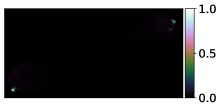
(a) Ground truth (linear scale)

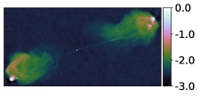
(b) Ground truth

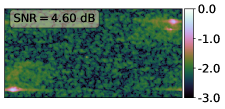
(c) Dirty reconstruction

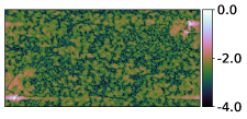
(d) Dirty reconstruction error

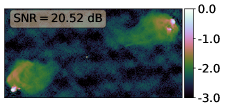
(e) MMSE reconstruction

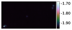
(f) Posterior standard deviation

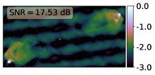
(g) MAP reconstruction

(h) MAP reconstruction error

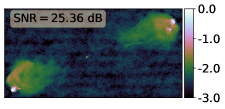
(i) MMSE reconstruction

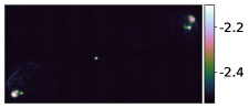
(j) Posterior standard deviation

(k) MAP reconstruction

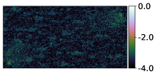
(l) MAP reconstruction error

Figure 4: RI image reconstructions for Cygnus A. The order of the images follows the M31 results presented in Figure 1. Compared with the wavelet-based model, QuantifAI recovers a reconstruction with a higher SNR and shows more meaningful uncertainties, which can be seen by comparing the posterior standard deviation and the MAP reconstruction error.

The base images used in our experiment are the ones from Cai et al. (2018a): (i) the HI region of the M31 galaxy in Figure 1 (a), (ii) the W28 supernova remnant in Figure 2 (a), (iii) the 3C288 radio galaxy in Figure 3 (a), and (iv) the Cygnus A radio galaxy in Figure 4 (a). All the images are $256\times 256$ pixels, except for the Cygnus A galaxy, which is $256\times 512$. As the ground truth images are reconstructed from real observations, there are minor original residuals and backgrounds that are more noticeable in the log scale images, for example, see Figure 3 (b).

The previous images correspond to $\bm{x}$ in our observational model from Equation 3. The complex Gaussian noise $\bm{n}\in\mathbb{C}^{M}$ is composed of independent and identically distributed (i.i.d.) samples. Each sample is simulated following a complex Gaussian distribution, $n_{i}\sim\mathcal{N}_{\mathcal{C}}(0,\sigma^{2})$, which implies that $\text{Re}(\bm{n}),\text{Im}(\bm{n})\sim\mathcal{N}(0,\sigma/\sqrt{2})$ (Tse & Viswanath, 2005). The noise is set such that we get a specific input signal-to-noise ratio (ISNR) on each image. For all the experiments, we set the ISNR to $30$dB, and the noise standard deviation is computed as follows

$$\sigma=\frac{\|\bm{\Phi}\bm{x}\|_{2}}{\sqrt{M}}\,10^{-\text{ISNR}/20}\,.$$ (50)

To mimic the $uv$ plane coverage, we reuse the Fourier mask from Cai et al. (2018a, Fig. 2) and use it to generate the visibilities from $\bm{y}$. The variable sampling density profile was taken from Puy et al. (2011) and represents a $10\%$ coverage of the Fourier plane.

5.2 Models and experiment settings

5.2.1 RI imaging models

The CRR-NN in the QuantifAI model is a pretrained model with $t=5$, Gaussian white noise with standard deviation $\sigma=5$, and parameters $\mu=20$ , $\lambda=5\times 10^{4}$. The model was trained on a set of natural images from the BSD500 dataset (Arbeláez et al., 2011) scaled to the $[0,255]$ range, using $\ell_{1}$ norm as the loss function in Equation 22 with the Adam optimiser (Kingma & Ba, 2017). The training parameters followed Goujon et al. (2023b, §VI.A).

The wavelet dictionary $\Psi$ used in the wavelet-based model is composed of Daubechies $8$ wavelets (Daubechies, 1992) with a multiresolution level $J=4$ following the setup from Cai et al. (2018a, b). The regularisation parameter $\lambda_{\text{\scriptsize WAV}}$ was set to $1\times 10^{2}$.

The regularisation strengths of both models, $\lambda$ and $\lambda_{\text{\scriptsize WAV}}$, were set to maximise the MAP reconstruction SNR using a grid search. We observed that QuantifAI’s reconstruction SNR is significantly more robust with respect to the choice of regularisation strength than the wavelet-based models.

5.2.2 Optimisation settings

For QuantifAI, we used the optimisation algorithm shown in Algorithm 1. The wavelet-based model also requires a proximal algorithm due to its non-smooth component and to provide a fair comparison we used the FISTA algorithm (Beck & Teboulle, 2009). In these experiments, we assumed that the noise level $\sigma$ is known. If the noise level is unknown, it may be estimated by standard techniques (Price et al., 2021b). Both algorithms’ tolerance criterion $\xi$ was set to $10^{-5}$, and the total number of iterations to $1.5\times 10^{4}$. Nevertheless, both optimisation algorithms converged before the total number of iterations was reached.

5.2.3 MCMC sampling settings

We generate $5\times 10^{4}$ samples from each posterior distribution, with $5\times 10^{4}$ burn-in iterations and a thinning factor of $10$. The burn-in iterations consist of generating several samples that will be discarded so that the chain passes its transient period. The thinning factor corresponds to the number of samples that need to be generated between two samples so that they can be considered independently drawn from the target distribution. The sampling algorithm produced a total of $5.5\times 10^{5}$ samples for each model. We have set to $10$ the number of stages for the SK-ROCK algorithm (Pereyra et al., 2020), which is one of its main hyperparameters. The sampling of the posterior probability distributions is used as a validation, and therefore we set the sampling parameters focusing on good reconstructions and posterior samples rather than speed.

The wavelet-based model requires the MY envelope approximation to guarantee the chain’s convergence, as described in Section 2.5.3 and Section 4.3. The MY approximation parameter $\gamma$ was set to the inverse of the likelihood gradient’s Lipschitz constant, c.f. the first term of Equation 28.

The choice of the step sizes is critical to ensure the chains’ convergence to the target distribution in a reasonable amount of time. The step size is chosen as a function of each posterior gradient’s Lipschitz constant. The step sizes $\delta_{\textsc{Q}}$ and $\delta_{\text{W}}$, corresponding to the QuantifAI and wavelet-based models, respectively, are computed as follows

$$\delta_{\textsc{Q}}=\frac{\kappa_{\textsc{Q}}}{L_{\text{likelihood}}+L_{\text{prior-CRR-NN}}}\,,\quad\delta_{\text{W}}=\frac{\kappa_{\text{W}}}{L_{\text{likelihood}}+\gamma^{-1}}\,,$$ (51)

where the Lipschitz constant bounds are shown in Equation 28, and $\kappa_{\textsc{Q}}$ and $\kappa_{\text{W}}$, are two positive constants smaller than one, here set to $0.98$. We have followed the advise from Durmus et al. (2018); Cai et al. (2018a) to set the sampling parameters.

5.2.4 UQ settings

We set $\alpha=0.01$ in all the UQ methods, so the confidence level is $99\%$. We used the bisection algorithm to compute the LCIs and the fast pixel UQ at different scales, with tolerance $10^{-4}$ and maximum number of iterations $200$, for both models. We used the same wavelet dictionary as in the wavelet-based model for the fast pixel UQ at different scales.

The inpainting algorithm uses the same stopping criterion as Algorithm 1. In this case, the tolerance is set to $5\times 10^{-6}$, and the total number of iterations to $1.5\times 10^{4}$. The CRR-NN used for the inpainting is the same one used in the QuantifAI model.

The Gaussian blurring kernel $G(0,\Sigma)$ from Equation 35 is set using $\Sigma=\sigma_{G}^{2}I_{2\times 2}$, with $\sigma_{G}$ being $3.5$ pixels and a truncation radius of $7$ pixels, giving a kernel $G\in\mathbb{R}^{15\times 15}$.

5.3 Image reconstruction

Table 1: Reconstruction performance of the different point estimates for the dataset images in terms of SNR with respect to the ground truth. We compare the MAP and the MMSE reconstruction of the wavelet-based and the QuantifAI model. We include the dirty reconstruction as a reference. We observe that the MAP estimation from QuantifAI outperforms the other reconstructions from the wavelet-based prior and all the MMSE estimations.

Images	Reconstruction SNR [dB]
	Dirty	Wavelet-based prior		QuantifAI
		MMSE	MAP	MMSE	MAP
W28	$3.39$	$18.17$	$23.04$	$23.38$	$\bf 26.85$
M31	$5.01$	$23.78$	$25.52$	$24.61$	$\bf 27.48$
3C288	$7.02$	$14.31$	$14.15$	$23.23$	$\bf 24.10$
Cygnus A	$4.60$	$20.52$	$17.53$	$25.36$	$\bf 30.25$

We present the RI image reconstructions of the four ground truth test images in Figure 1, Figure 2, Figure 3 and Figure 4. In each figure, we compare the wavelet-based and QuantifAI models, and we include the dirty reconstruction as a reference. The metric used to compare the RI image reconstruction is the SNR expressed in dB defined as follows

$$\text{SNR}(\bm{x},\bm{x}_{\text{gt}})=-20\log_{10}\left(\frac{\|\bm{x}_{\text{gt}}-\bm{x}\|_{2}}{\|\bm{x}_{\text{gt}}\|_{2}}\right)\,,$$ (52)

where $\bm{x}_{\text{gt}}$ corresponds to the reference or ground truth, and $\bm{x}$ to the estimation, and $\|\cdot\|_{2}$ is the usual $\ell_{2}$ norm.

The quantitative reconstruction performance results are presented in Table 1. The MAP reconstruction from QuantifAI performs significantly better than the wavelet-based counterpart in every image from our dataset. The performance gain lies between $1.9$dB and $12.7$dB, with an average gain of $7$dB. It is difficult to see the QuantifAI improvements by eye when inspecting reconstructed images. However, when observing the errors in the fourth column, the improved quality of QuantifAI’s reconstructions becomes evident. Shifting towards the sampling results, we observe a similar behaviour of the MMSE reconstruction in favour of QuantifAI’s images. The MAP is considerably faster than the MMSE, relying on optimisation rather than posterior sampling. In addition, the MAP consistently provides improved reconstruction performance with respect to the MMSE.

The posterior standard deviation provides a qualitative way to validate the posterior model and its uncertainties. The comparison of the posterior standard deviation with the MAP reconstruction error shows a higher correlation for the QuantifAI model than the wavelet-based model. In addition, the posterior standard deviation of QuantifAI shows lower variance than its wavelet-based counterpart, which is in agreement with QuantifAI’s smaller reconstruction error. For example, in image W28 in Figure 2, we observe in subfigure (2(j)) that the posterior standard deviation value is large near the edges of the ground truth image. It is reassuring that QuantifAI’s reconstruction error also shows the same behaviour.

The performance results showcase the expressive power of the CRR-NN-based prior even if the regulariser is constrained to be convex. The results also confirm the generalisation power of the CRR-NN-based prior. Even if trained on natural images, the CRR-NN can provide remarkable reconstruction performances for astronomical images and meaningful posterior standard deviations.

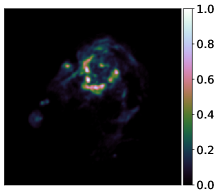
(a) Ground truth (linear scale)

(b) Ground truth

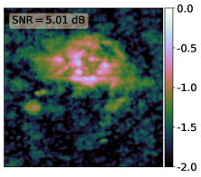
(c) Dirty reconstruction

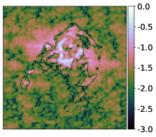
(d) Dirty reconstruction error

(e) MMSE reconstruction

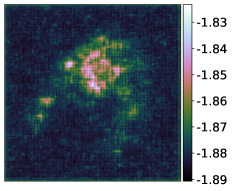
(f) Posterior standard deviation

(g) MAP reconstruction

(h) MAP reconstruction error

(i) MMSE reconstruction

(j) Posterior standard deviation

(k) MAP reconstruction

(l) MAP reconstruction error

Figure 1: RI image reconstructions for M31. The images are shown in a $\log_{10}$ scale except for subfigure (a). Top row: The first two images show the ground truth intensity image in linear and $\log_{10}$ scales, respectively. The third image shows the dirty reconstruction, computed by applying the pseudo-inverse of the measurement operator on the observations. The fourth image shows the error of the dirty reconstruction with respect to the ground truth. Middle row: We show the results of the wavelet-based model. The first and second columns show the minimum mean squared error (MMSE) estimator and the posterior standard deviation, respectively. Both images are computed using the $5\times 10^{4}$ generated posterior samples. The third column shows the MAP reconstruction obtained through an optimisation algorithm. The fourth column depicts the error of the MAP reconstruction with respect to the ground truth. Bottom row: We present the results of the QuantifAI model. The columns are presented in the same order as for the Wavelet reconstructions in the middle row. For every reconstruction, we display the SNR with respect to the ground truth in the top left corner. Compared with the wavelet-based model, QuantifAI recovers a reconstruction with a higher SNR and shows more meaningful uncertainties, which can be seen by comparing the posterior standard deviation and the MAP reconstruction error.

(a) Ground truth (linear scale)

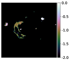
(b) Ground truth

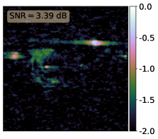
(c) Dirty reconstruction

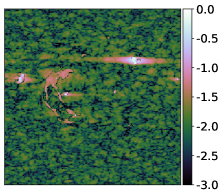
(d) Dirty reconstruction error

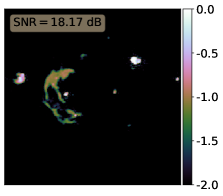
(e) MMSE reconstruction

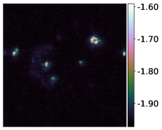
(f) Posterior standard deviation

(g) MAP reconstruction

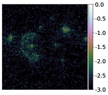
(h) MAP reconstruction error

(i) MMSE reconstruction

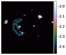
(j) Posterior standard deviation

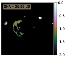
(k) MAP reconstruction

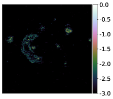
(l) MAP reconstruction error

Figure 2: RI image reconstructions for W28. The order of the images follows the M31 results presented in Figure 1. Compared with the wavelet-based model, QuantifAI recovers a reconstruction with a higher SNR and shows more meaningful uncertainties, which can be seen by comparing the posterior standard deviation and the MAP reconstruction error.

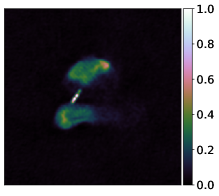
(a) Ground truth (linear scale)

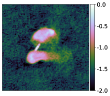
(b) Ground truth

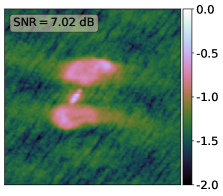
(c) Dirty reconstruction

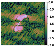
(d) Dirty reconstruction error

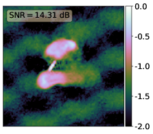
(e) MMSE reconstruction

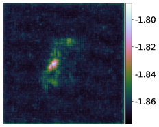
(f) Posterior standard deviation

(g) MAP reconstruction

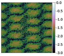
(h) MAP reconstruction error

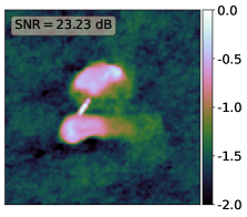
(i) MMSE reconstruction

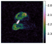
(j) Posterior standard deviation

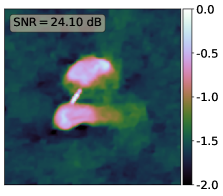
(k) MAP reconstruction

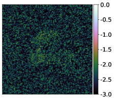
(l) MAP reconstruction error

Figure 3: RI image reconstructions for 3C288. The order of the images follows the M31 results presented in Figure 1. Compared with the wavelet-based model, QuantifAI recovers a reconstruction with a higher SNR and shows more meaningful uncertainties, which can be seen by comparing the posterior standard deviation and the MAP reconstruction error.

5.4 Hypothesis testing of image structure

We start by carrying out hypothesis tests of image structure, which are the most scalable UQ techniques we will study. First, a surrogate image is created by modifying one region of interest. It only takes one further evaluation of the likelihood and prior potential to carry out the hypothesis test. The test helps to quantitatively answer a scientific question with a $100(1-\alpha)\%$ confidence level. The scientific question targeted depends on the constructed surrogate image, and in this work, we consider two scenarios.

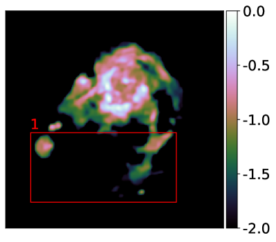
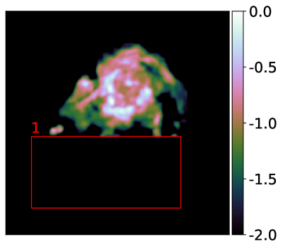
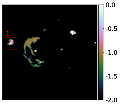
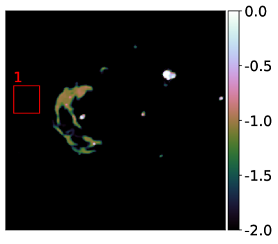
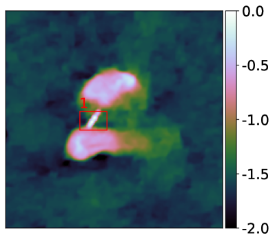
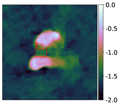
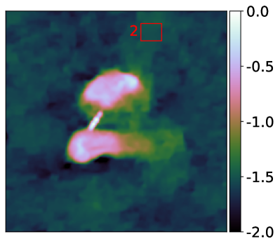
(a) MAP reconstruction	(b) Inpainted surrogate

Figure 5: Hypothesis test of different regions of the four QuantifAI MAP reconstructions for M31, W28, Cygnus A, and 3C288. All the images are shown in $\log_{10}$ scale. The left column shows the respective MAP reconstruction with the region of interest framed in a red rectangle. The right column shows the surrogate images inpainted using the QuantifAI prior. The first four rows show regions corresponding to physical structures present in the ground truth images. The last row corresponds to a non-physical region. Results of the hypothesis tests are summarised in Table 2.

In the first scenario, we consider a particular structure in the reconstructed intensity image. We can query whether the structure’s origin is physical or not. For example, the structure could be a reconstruction artefact or a physical process. Figure 5 shows this option, where we have analysed different regions of the four images. The first four inpainted regions correspond to physical structures, and the fifth region, i.e., region number $2$ of image 3C288, does not correspond to a physical structure. The surrogate images are produced with an inpainting algorithm using QuantifAI’s prior so that the inpainted region agrees with the prior.

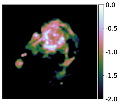
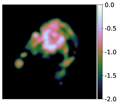
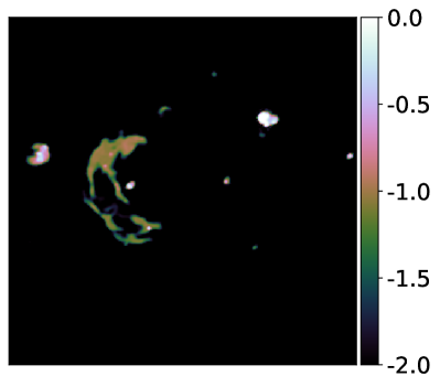
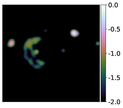
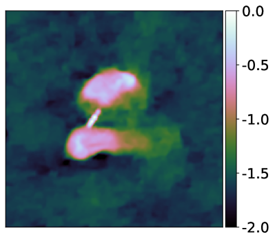
(a) MAP reconstruction	(b) Blurred surrogate

Figure 6: Hypothesis test of the fine structure in the four QuantifAI MAP reconstructions for M31, W28, Cygnus A, and 3C288. All the images are shown in $\log_{10}$ scale. The fine structure is blurred using a Gaussian kernel with a standard deviation of $3.5$ pixels and a radius of $7$ pixels. The blurred surrogate images in the second column are constructed by blurring the MAP reconstruction shown in the first column. The hypothesis tests are done with the QuantifAI model.

The second scenario is to blur the finer structure in the reconstructed image and perform a hypothesis test to elucidate the question of whether the blurred structure is physical or not. The test is illustrated in Figure 6. In this case, all four blurred images represent physical structures.

In both cases, we compare the hypothesis test using a MAP-based approach described in this work and a sampling-based approach for validation. In the MAP-based approach, we build the HPD region in Equation 31 with the approximation in Equation 32 and use the MAP estimation as our reconstruction. In the sampling-based approach, we use the MMSE as the reconstruction, i.e., the mean of the posterior samples, and compute the threshold defining the HPD region using the quantile function on the potentials of the posterior samples following Cai et al. (2018a, §5.2).

Table 2: Hypothesis test results for the inpainted surrogates in Figure 5 using the QuantifAI model. The function $(f+g)(\cdot)$ corresponds to the combined potential of the likelihood and the prior. The reconstruction $\hat{\bm{x}}^{*}$ represents the point estimate used in the sampling or optimisation scenarios, which are the MMSE and the MAP, respectively. The SK-ROCK method corresponds to the posterior sampling techniques. The image $\hat{\bm{x}}^{*,{\text{sgt}}}$ corresponds to the surrogate image, where the areas of interest shown in Figure 5 have been inpainted. The isocontours, $\hat{\gamma}_{0.01}$, or threhsolds, are calculated with an $\alpha$ of $0.01$ giving a credible set of $99\%$. In the MAP row, the threshold is computed following the approximation in Equation 32. In the SK-ROCK row, the threshold is computed from the posterior samples following Cai et al. (2018a). The symbols  ✓  and  ✗  in the Ground truth column indicate if the inpainted region contains a physical structure from the ground truth or not, respectively. In the last column, the  ✓  indicates that the hypothesis test is conclusive. All values are scaled with $10^{5}$. QuantifAI is able to correctly reject the hypothesis for all images where the tested structure is physical except for the Cygnus A image. In all cases, the MAP-based and MCMC sampling-based results agree with each other.

Images	Test	Ground	Method	Point estimate	Surrogate	Isocontour	Hypothesis
	area	truth		$(f+g)(\hat{\bm{x}}^{*})$	$(f+g)(\hat{\bm{x}}^{*,{\text{sgt}}})$	$\hat{\gamma}_{0.01}$	test
M31	1	✓	SK-ROCK	$0.340$	$\bf 1.159$	$0.742$	✓
			MAP	$0.310$	$\bf 1.161$	$0.990$	✓
Cygnus A	1	✓	SK-ROCK	$0.125$	$0.182$	$\bf 0.848$	✗
			MAP	$0.105$	$0.169$	$\bf 1.450$	✗
W28	1	✓	SK-ROCK	$0.222$	$\bf 4.649$	$0.612$	✓
			MAP	$0.196$	$\bf 4.699$	$0.876$	✓
3C288	1	✓	SK-ROCK	$0.257$	$\bf 1.918$	$0.659$	✓
			MAP	$0.229$	$\bf 1.908$	$0.908$	✓
2-8	2	✗	SK-ROCK	$0.257$	$0.257$	$\bf 0.659$	✗
			MAP	$0.229$	$0.229$	$\bf 0.908$	✗

Table 2 presents the results for the inpainting hypothesis test, where the inpainted surrogates are shown in Figure 5. The MAP- and sampling-based results are consistent in all the images studied, where the threshold computed with the posterior samples is slightly tighter than the MAP-based approximation. The hypothesis tests correctly classify the structure in images M31, W28 and 3C288, including the two cases of the latter image. The UQ methods cannot make a strong statistical statement about the structures in the Cygnus A image. In this image, where the inpainted region has a tiny physical structure, the potentials of the inpainted surrogate image rest close to the MAP and MMSE estimators. We include the hypothesis test results of the same inpainting experiment for the wavelet-based model in Appendix A.1 to provide a comparison between the models. We used the wavelet prior to inpaint the region of interest to allow for a fair comparison. All results from the wavelet-based model are in agreement with QuantifAI.

Table 3: Hypothesis test results for the blurred surrogates of Figure 6 using the QuantifAI model. The description of Figure 6 holds in this table. All values are scaled with $10^{5}$. QuantifAI is able to correctly reject the hypothesis in all cases, and the MAP-based outcome agrees with its MCMC sampling-based counterpart.

Images	Method	Initial	Surrogate	Isocontour	Hypothesis
		$(f+g)(\hat{\bm{x}}^{*})$	$(f+g)(\hat{\bm{x}}^{*,{\text{sgt}}})$	$\hat{\gamma}_{0.01}$	test
M31	SK-ROCK	$0.340$	$\bf 1.905$	$0.742$	✓
	MAP	$0.310$	$\bf 1.906$	$0.990$	✓
Cygnus A	SK-ROCK	$0.125$	$\bf 9.642$	$0.848$	✓
	MAP	$0.105$	$\bf 9.643$	$1.450$	✓
W28	SK-ROCK	$0.222$	$\bf 8.389$	$0.612$	✓
	MAP	$0.196$	$\bf 8.387$	$0.876$	✓
3C288	SK-ROCK	$0.257$	$\bf 0.920$	$0.659$	✓
	MAP	$0.229$	$\bf 0.922$	$0.908$	✓

The results from the blurred surrogates of Figure 6 are presented in Table 3. In all the images, the hypothesis test concludes that the blurred fine structure is physical as the potential falls out of the HPD region. The MAP- and sampling-based results are consistent with each other.

The different hypothesis tests have shown consistent results between the sampling-based and highly scalable MAP-based results. In addition, the results from the hypothesis tests are coherent between the QuantifAI and wavelet-based model. We remark that the approach based on the MAP requires one further measurement operator evaluation to carry out the hypothesis test. The test provides a highly scalable way to answer scientific questions about the uncertainty of the RI imaging reconstructions.

5.5 Local credible intervals

We have exploited the approximation of the HPD region from Section 4.1 based on the MAP estimations and a credible level of $99\%$. The approximate HPD regions were then used to compute the LCIs, whose lengths per pixel are visualized as an image, c.f. Figure 7. The LCI lengths are displayed after subtracting the mean LCI length overall superpixels in the image, which is shown in the top left corner of the image. The UQ results for QuantifAI are presented for two superpixel sizes, $4\times 4$ and $8\times 8$. We have omitted LCIs from the wavelet-based prior for conciseness. The posterior standard deviations at the two superpixel sizes are included for comparison with the significantly faster MAP-based UQ technique of the LCIs. We find a reasonable agreement between the structure in the LCI plots and the posterior standard deviation. For example, the 3C288 image with superpixel size $8\times 8$ yields tighter LCIs in the two elliptical regions and in the small connecting structure in the centre of the image. The corresponding posterior standard deviation is smaller in the aforementioned regions, which is expected as most of the observed signal concentrates there. The LCIs and the posterior standard deviation represent different quantiles, so we would not expect an exact agreement even without any approximation in the computation of the LCIs.

We observe, as expected, that the larger superpixels have tighter LCIs, as seen in the mean LCIs shown on the top left corner of the subfigures in Figure 7. The reconstructions are naturally less uncertain on the larger scales due to the properties of our measurement operator, as the visibilities are generally concentrated towards the low frequencies. In addition, varying the value of a larger superpixel saturates the HPD region faster than for a small superpixel. We have also computed the LCIs for the superpixels of size $16\times 16$, which we have not included for conciseness. The corresponding mean LCI values are $0.20$, $0.08$, $0.24$, and $0.07$ for the images in the same order as in Figure 7.

When comparing the mean value of the LCIs from the four reconstructions from Figure 7 we notice that two of them, M31 and 3C288, have higher uncertainty than the rest. The higher the uncertainty, the larger the mean value of the LCI gets, as the superpixel values need larger changes before they saturate the HPD region. Image 3C288, with a superpixel size of $4\times 4$, is an example where the LCIs have saturated as the mean is close to unity; therefore, the LCI image’s detailed structure is lost due to the saturation. This saturation highlights the need for superpixel sizes to be selected appropriately, depending on the case at hand.

M31	W28	3C288	Cygnus A
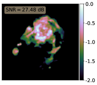
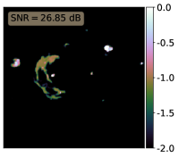
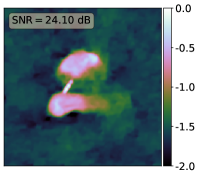
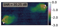
Superpixel size: $4\times 4$
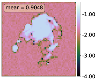
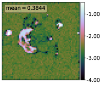
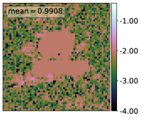
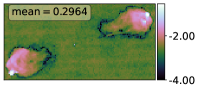
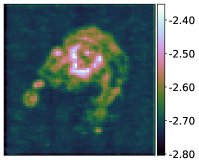
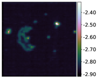
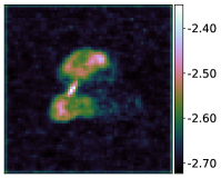
Superpixel size: $8\times 8$

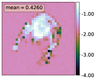
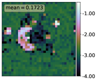
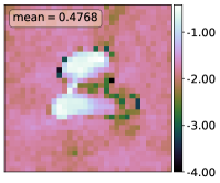
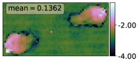
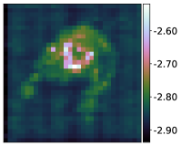
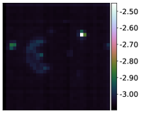
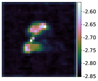
Figure 7: Length of the local credible intervals (LCIs), cf. Bayesian error bars, computed with a $99\%$ credible level using superpixel sizes of $4\times 4$ and $8\times 8$. Each column represents one of the four images in our dataset. The first row shows the MAP estimation of each image at its original resolution. The second row displays the variation of the LCIs around their mean, recorded in a box in the upper left corners. This display choice allows us to visualise the structure of the LCIs better while keeping the LCIs mean information. The third row presents the posterior standard deviation computed with the same superpixel size. The fourth and fifth rows present the equivalent information for the superpixel size of $8\times 8$. There is reasonable agreement between the uncertainty captured by the LCI and the posterior standard deviation.

5.6 Fast pixel uncertainty quantification at different scales

The fast pixel UQ method results for the images M31 and W28 are reported in Figure 8. We use the error between the MAP estimation and the ground truth image, i.e., true error, to validate the predicted uncertainty of the fast UQ method. The true error at different scales can be computed following Equation 45,

$$\hat{\bm{x}}_{\text{GT},\,j}=\sum_{\begin{subarray}{c}l=0,\\ l\neq j\end{subarray}}^{J}\mathbf{\Psi}_{l}\,\bm{a}_{\text{GT},l}+\mathbf{\Psi}_{j}\hat{\bm{a}}_{\text{MAP},\,j}\,,$$ (53)

where $\bm{a}_{\text{GT},l}$ are the wavelet decomposition coefficients of the ground truth image at multi-resolution level $l$. We have replaced the ground truth image’s wavelet coefficient at a single level with the coefficients from the MAP reconstruction.

We observe a good agreement between the predicted and ground truth errors at the different multi-resolution levels. There is an overestimation of the errors, which can come from two sources. First, the approximation of the HPD region is conservative, as it has been discussed in Pereyra (2017). Second, the MAP estimation is already missing some of the fine or high-frequency structures in the ground truth images. This fact can be seen in the MAP reconstruction errors in subfigures 1(h) and 2(h). The missing high-frequency structure is expected due to the properties of the measurement operator discussed in Section 2.1.

The structure from the chosen wavelet representation, $\mathbf{\Psi}$, underpinning the UQ method can be observed in the predicted errors. This structure is visible mainly in the higher frequencies of the W28, where point sources are in the image. The wavelet structure should be taken into account when analysing the reconstruction errors.

This fast pixel UQ method allows us to approximate the reconstruction errors made at different scales for a fraction of the computational cost of the LCI pixel UQ method. The evaluations of the measurement operators are reduced by three orders of magnitude, resulting in an ultra-fast and truly scalable pixel UQ method. Furthermore, a single nonlinear equation solve, e.g. root finding problem, of the new pixel UQ method suffices to predict the errors at all scales, while with LCIs, we are required to repeat the process for each superpixel size.

M31		W28
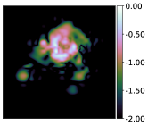
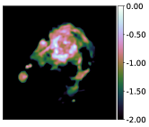
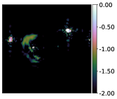
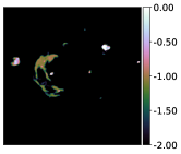
(a) Thresholded MAP	(b) MAP estimation	(c) Thresholded MAP	(d) MAP estimation
Errors		Errors
Predicted	True errors	Predicted	True errors

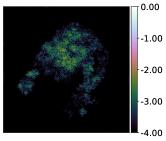
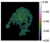
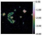
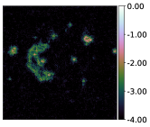
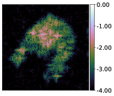
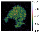
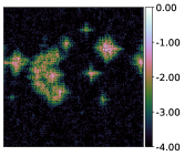
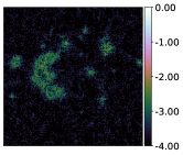
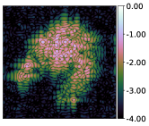
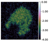
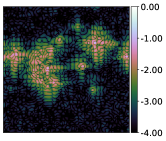
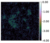
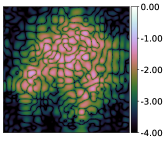
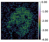
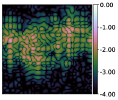
Figure 8: Fast pixel uncertainty quantification (UQ) with the QuantifAI model on the images M31 and W28. The first two columns correspond to M31, while the last two columns to W28. The first row displays the pairs of the thresholded MAP reconstruction that saturates the HPD region versus the original MAP reconstruction. The following rows compare the predicted error of the thresholded MAP computed with the fast pixel UQ method against the MAP reconstruction error using ground truth images at each wavelet scale. The last row shows the cumulative error when considering all scales.

5.7 Computation time

The computation wall-clock time for both models, QuantifAI and the wavelet-based, are summarised in Table 4. All the computations for both models were done using an Nvidia-A100 40GB GPU using Pytorch (Paszke et al., 2019). We observe a lower computation time for the QuantifAI model with respect to its wavelet-based counterpart. One reason is the lightweight CRR-NN model that quickly evaluates its gradient and potential. Note that the regularisation strength has an impact on the number of iterations and it could be changed to favour a faster convergence. The regularisation strength was chosen to optimize MAP reconstruction quality.

The results shown in Table 4 highlight the importance of relying on optimisation-based rather than sampling-based reconstructions when focusing on the scalability of the method. There is a difference of approximately four orders of magnitude in the computation time of the MAP and the MMSE which relies on MCMC sampling techniques. Focusing on UQ, the posterior sampling is $60$ times slower than the computation of the LCIs with $8\times 8$ superpixels and more than $37500$ times slower than the fast pixel UQ proposed in this work. The new fast pixel UQ provides an extremely rapid approach to providing pixel-based UQ, over $630$ times faster than the $8\times 8$ LCIs.

The evaluation of the measurement operator is the most time-consuming operation in a real large-scale RI imaging scenario. If we target scalability, we need to monitor the number of measurement operator evaluations. Table 5 summarises the number of measurement operator evaluations required for the UQ techniques. The results are only shown for the QuantifAI model as they are representative of the wavelet-based model. As mentioned before, we note the reduction of evaluations between optimisation and sampling-based reconstructions. We remark on the reduction in the number of evaluations for the UQ tasks, approximately $3$ orders of magnitude between the sampling and the LCIs, and $3$ subsequent orders of magnitude between the LCIs and the fast pixel UQ. These results make the fast pixel UQ $6$ orders of magnitude faster than MCMC sampling. The MAP estimation for the CRR required $1082$ measurement operator evaluations. However, the algorithm’s settings were chosen to maximise the reconstruction SNR. By modifying the regularisation parameter of the CRR-based prior, we can reduce the number of evaluations by an order of magnitude. Recent developments in code parallelisation for RI imaging reconstruction algorithms (Pratley et al., 2019a; Pratley & McEwen, 2019) could be integrated to push the scalability of the method further.

Table 4: Computation wall-clock times for the W28 image in seconds for both models being compared.

Models	MAP	Posterior	LCIs	Fast
	optim.	sampling	$8\times 8$	pixel UQ
Wavelet-based	$0.94$	$36.0\times 10^{3}$	$149.7$	—
QuantifAI	$0.64$	$6.44\times 10^{3}$	$108.2$	$0.17$

Table 5: The number of measurement operator evaluations used by the QuantifAI for the W28 image. We do not distinguish between the measurement operator and its adjoint. Therefore, evaluating the log-likelihood gradient counts as two evaluations of the measurement operator. The fast pixel UQ is three and six orders of magnitude faster than the MCMC sampling and LCIs, respectively.

MCMC	LCIs	LCIs	Fast
sampling	$8\times 8$	$16\times 16$	pixel UQ
$11\times 10^{6}$	$81.5\times 10^{3}$	$21.2\times 10^{3}$	$28$

6 Conclusions

In this work, we propose a new method coined QuantifAI that addresses uncertainty quantification in radio-interferometric (RI) imaging with data-driven (learned) priors in very high-dimensional settings. We have focused on three fundamental points in the RI imaging pipeline: scalability, estimation performance, and uncertainty quantification (UQ).

Our model builds upon a principled Bayesian framework for the UQ analysis, which is known to be computationally expensive when exploiting MCMC sampling methods. However, in this work, we leverage convex optimisation techniques to estimate the maximum-a-posteriori (MAP), the point estimate of the posterior distribution we use as reconstruction. We restrict our model to a log-concave posterior distribution to remain highly scalable and have Bayesian UQ techniques. This restriction is equivalent to having convex potentials for our likelihood and prior. In this scenario, we can exploit an approximation of the high posterior density (HPD) region, which only requires the MAP estimation (Pereyra, 2017) and bypasses expensive sampling techniques.

We want to include data-driven priors that can encode complex information learned implicitly from training data making them more expressive. Consequently, the learned priors allow us to improve performance with respect to previous models based on handcrafted priors (Cai et al., 2018b), e.g., wavelet-based sparsity-promoting priors. To support fast UQ techniques, our models must be convex, hence we adopt the recently introduced learnable convex-ridge regulariser neural network (CRR-NN, Goujon et al., 2023b). The CRR-NN-based prior is performant, reliable and has shown to be robust to data distribution shifts. The QuantifAI model uses an analytic physically motivated model for the likelihood and the learned CRR-NN-based prior. In this work we are focusing on the methodology, which is why we have only considered small problems, i.e., images of $256\times 256$. Nevertheless, QuantifAI can be integrated into the distributed frameworks (Pratley et al., 2019a; Pratley & McEwen, 2019), which is the focus of ongoing work.

Numerical experiments are conducted with four images representative of RI imaging. We compare the QuantifAI model with the model containing a wavelet-based prior of Cai et al. (2018b). Our results show a considerable improvement in the reconstruction performance for QuantifAI. We validate our results against posterior samples from MCMC sampling algorithms and compute the posterior standard deviation. We found that QuantifAI produced more meaningful posterior standard deviations in comparison to the wavelet-based model.

We explore several MAP-based UQ techniques that rely on the approximate HPD region. We carry out hypothesis tests of image structure to asses if some structures observed in the reconstructions are physical. We then computed local credible intervals (LCIs c.f. Bayesian error bars) to measure the pixel-wise uncertainty. These two approaches were proposed by Cai et al. (2018b), and in this work, we validated them with MCMC posterior sampling results. Even if LCIs represent an already scalable alternative to sampling-based methods to provide pixel-wise UQ, they remain expensive for SKA-size data. Therefore, we proposed a novel pixel-wise UQ technique to approximate pixel errors at different scales that is three orders of magnitude faster than the LCIs. The new approach is based on thresholding the coefficients of a wavelet representation of the reconstruction until the HPD region saturates and is six orders of magnitude faster than sampling-based techniques.

QuantifAI represents a highly scalable and performant approach to address UQ in RI imaging. In this work, we have compared QuantifAI to a wavelet-based model using numerical experiments and a variety of metrics. However, as both models rely on the Bayesian framework, we could make a Bayesian model comparison, a principled approach to model selection and determine which model the data favours. Recent developments in McEwen et al. (2023) extend the model comparison to the learnt setting, with data-driven priors. The focus of ongoing work is to implement the proposed methodology in existing RI imaging frameworks purify (Carrillo et al., 2014; Pratley et al., 2018; Pratley et al., 2019b) and sopt (Carrillo et al., 2012; Onose et al., 2016) to exploit massively parallelised computing environment (Pratley et al., 2019a; Pratley & McEwen, 2019). In the near future, we plan to benchmark the speed and scalability of QuantifAI in a highly realistic setting.

A new perspective is to relax the convexity constraint of the prior by exploiting the fact that the posterior potential needs to be convex (rather than the prior) and that the RI imaging likelihood is already strongly convex. The relaxation of the CRR regulariser has been studied in a very recent work (Goujon et al., 2023a), where a weakly-convex-ridge-regulariser neural network (WCRR-NN) has been proposed. If the WCRR-NN is adopted, it could further enhance the expressiveness of the regulariser and the reconstruction performance of QuantifAI in the RI imaging problem.

Data Availability

We provide the QuantifAI PyTorch-based Python package in a publicly available repository. The images, scripts, trained CRR-NN model and code to reproduce this article’s experiments can be found in the aforementioned repository.

Appendix A Wavelet-based Bayesian uncertainty quantification

A.1 Hypothesis testing of image structure

Figure 9 and Table 6 present the results of the hypothesis testing of structure for the model with the sparsity-promoting prior.

Table 6: Hypothesis test results for the inpainted surrogates from Figure 9 generated with the wavelet-based model. All values are in units $10^{4}$. The description of Table 2 applies in this table.

Images	Test	Ground	Method	Initial	Surrogate	Isocontour	Hypothesis
	area	truth		$(f+g)(\hat{\bm{x}}^{*})$	$(f+g)(\hat{\bm{x}}^{*,{\text{sgt}}})$	$\hat{\gamma}_{0.01}$	test
M31	1	✓	SK-ROCK	$0.448$	$\bf 1.396$	$1.105$	✓
			MAP	$0.359$	$\bf 1.335$	$1.039$	✓
Cygnus A	1	✓	SK-ROCK	$0.480$	$0.533$	$\bf 1.639$	✗
			MAP	$0.444$	$0.514$	$\bf 1.789$	✗
W28	1	✓	SK-ROCK	$0.353$	$\bf 5.190$	$0.879$	✓
			MAP	$0.284$	$\bf 5.204$	$0.964$	✓
3C288	1	✓	SK-ROCK	$0.729$	$\bf 2.487$	$1.398$	✓
			MAP	$0.654$	$\bf 2.409$	$1.333$	✓
2-8	2	✗	SK-ROCK	$0.729$	$0.729$	$\bf 1.398$	✗
			MAP	$0.654$	$0.654$	$\bf 1.333$	✗

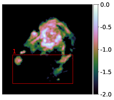
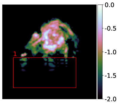
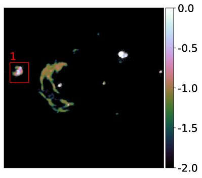
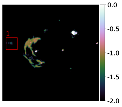
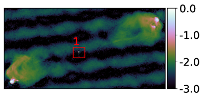
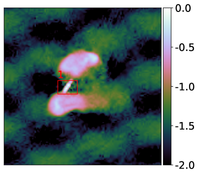
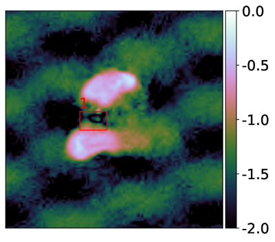
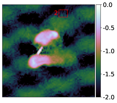
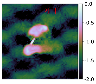
(a) MAP reconstruction	(b) Inpainted surrogate

Figure 9: Hypothesis test of different regions of the four images, M31, W28, Cygnus A, and 3C288. All the images are shown in $\log_{10}$ scale. The figure is similar to Figure 5, but the wavelet-based model has been used to generate the MAP. The wavelet prior was used to inpaint the surrogate image.

References

- Abdulle et al. (2018) Abdulle A., Almuslimani I., Vilmart G., 2018, SIAM/ASA Journal on Uncertainty Quantification, 6, 937
- Adler & Öktem (2018) Adler J., Öktem O., 2018, IEEE Transactions on Medical Imaging, 37, 1322
- Aghabiglou et al. (2023) Aghabiglou A., Terris M., Jackson A., Wiaux Y., 2023, in ICASSP 2023 - 2023 IEEE International Conference on Acoustics, Speech and Signal Processing (ICASSP). pp 1–5, doi:10.1109/ICASSP49357.2023.10094843
- Allam (2016) Allam T., 2016, Master’s thesis, University College London
- Amos et al. (2016) Amos B., Xu L., Zico Kolter J., 2016, arXiv e-prints, p. arXiv:1609.07152
- Arbeláez et al. (2011) Arbeláez P., Maire M., Fowlkes C., Malik J., 2011, IEEE Transactions on Pattern Analysis and Machine Intelligence, 33, 898
- Arridge et al. (2019) Arridge S., Maass P., Öktem O., Schönlieb C.-B., 2019, Acta Numerica, 28, 1
- Ashton et al. (2022) Ashton G., et al., 2022, Nature Reviews Methods Primers, 2, 39
- Astropy Collaboration et al. (2022) Astropy Collaboration et al., 2022, ApJ, 935, 167
- Beck & Teboulle (2009) Beck A., Teboulle M., 2009, SIAM Journal on Imaging Sciences, 2, 183
- Bhatnagar & Cornwell (2004) Bhatnagar S., Cornwell T. J., 2004, A&A, 426, 747
- Bohra et al. (2020) Bohra P., Campos J., Gupta H., Aziznejad S., Unser M., 2020, IEEE Open Journal of Signal Processing, 1, 295
- Boyd et al. (2011) Boyd S., Parikh N., Chu E., Peleato B., Eckstein J., 2011, Distributed Optimization and Statistical Learning via the Alternating Direction Method of Multipliers. now
- Braun et al. (2015) Braun R., Bourke T., Green J. A., Keane E., Wagg J., 2015, in Advancing Astrophysics with the Square Kilometre Array (AASKA14). p. 174, doi:10.22323/1.215.0174
- Burden & Faires (1989) Burden R. L., Faires J. D., 1989, Numerical Analysis, fourth edn. The Prindle, Weber and Schmidt Series in Mathematics, PWS-Kent Publishing Company, Boston
- Cai et al. (2018a) Cai X., Pereyra M., McEwen J. D., 2018a, Monthly Notices of the Royal Astronomical Society, 480, 4154
- Cai et al. (2018b) Cai X., Pereyra M., McEwen J. D., 2018b, Monthly Notices of the Royal Astronomical Society, 480, 4170
- Cai et al. (2022) Cai X., McEwen J. D., Pereyra M., 2022, Statistics and Computing, 32, 87
- Carrillo et al. (2012) Carrillo R. E., McEwen J. D., Wiaux Y., 2012, Monthly Notices of the Royal Astronomical Society, 426, 1223
- Carrillo et al. (2014) Carrillo R. E., McEwen J. D., Wiaux Y., 2014, Monthly Notices of the Royal Astronomical Society, 439, 3591
- Chambolle & Pock (2011) Chambolle A., Pock T., 2011, Journal of Mathematical Imaging and Vision, 40, 120
- Collaboration et al. (2019a) Collaboration T. E. H. T., et al., 2019a, The Astrophysical Journal Letters, 875, L1
- Collaboration et al. (2019b) Collaboration T. E. H. T., et al., 2019b, The Astrophysical Journal Letters, 875, L4
- Combettes & Pesquet (2009) Combettes P. L., Pesquet J.-C., 2009, arXiv e-prints, p. arXiv:0912.3522
- Condat (2013) Condat L., 2013, Journal of Optimization Theory and Applications, 158, 460
- Connor et al. (2022) Connor L., Bouman K. L., Ravi V., Hallinan G., 2022, MNRAS, 514, 2614
- Cornwell (2008) Cornwell T. J., 2008, IEEE Journal of Selected Topics in Signal Processing, 2, 793
- Dabbech, A. et al. (2015) Dabbech, A. Ferrari, C. Mary, D. Slezak, E. Smirnov, O. Kenyon, J. S. 2015, A&A, 576, A7
- Dabbech et al. (2018) Dabbech A., Onose A., Abdulaziz A., Perley R. A., Smirnov O. M., Wiaux Y., 2018, Monthly Notices of the Royal Astronomical Society, 476, 2853
- Daubechies (1992) Daubechies I., 1992, Ten Lectures on Wavelets. Society for Industrial and Applied Mathematics (https://epubs.siam.org/doi/pdf/10.1137/1.9781611970104), doi:10.1137/1.9781611970104, https://epubs.siam.org/doi/abs/10.1137/1.9781611970104
- Dewdney et al. (2009) Dewdney P. E., Hall P. J., Schilizzi R. T., Lazio T. J. L. W., 2009, Proceedings of the IEEE, 97, 1482
- Dong et al. (2016) Dong C., Loy C. C., He K., Tang X., 2016, IEEE Transactions on Pattern Analysis and Machine Intelligence, 38, 295
- Durmus et al. (2018) Durmus A., Moulines E., Pereyra M., 2018, SIAM Journal on Imaging Sciences, 11, 473
- Durmus et al. (2022) Durmus A., Moulines E., Pereyra M., 2022, SIAM Review, 64, 991
- Gheller & Vazza (2021) Gheller C., Vazza F., 2021, Monthly Notices of the Royal Astronomical Society, 509, 990
- Golub & van Loan (2013) Golub G. H., van Loan C. F., 2013, Matrix Computations, fourth edn. JHU Press, http://www.cs.cornell.edu/cv/GVL4/golubandvanloan.htm
- Goujon et al. (2023a) Goujon A., Neumayer S., Unser M., 2023a, arXiv e-prints, p. arXiv:2308.10542
- Goujon et al. (2023b) Goujon A., Neumayer S., Bohra P., Ducotterd S., Unser M., 2023b, IEEE Transactions on Computational Imaging, 9, 781
- Hallinan et al. (2019) Hallinan G., et al., 2019, in Bulletin of the American Astronomical Society. p. 255 (arXiv:1907.07648), doi:10.48550/arXiv.1907.07648
- Harris et al. (2020) Harris C. R., et al., 2020, Nature, 585, 357
- Hendrycks et al. (2020) Hendrycks D., et al., 2020, arXiv e-prints, p. arXiv:2006.16241
- Högbom (1974) Högbom J. A., 1974, A&AS, 15, 417
- Hunter (2007) Hunter J. D., 2007, Computing in Science & Engineering, 9, 90
- Kingma & Ba (2017) Kingma D. P., Ba J., 2017, Adam: A Method for Stochastic Optimization (arXiv:1412.6980)
- Klatzer et al. (2023) Klatzer T., Dobson P., Altmann Y., Pereyra M., María Sanz-Serna J., Zygalakis K. C., 2023, arXiv e-prints, p. arXiv:2308.09460
- Kloeden & Platen (2011) Kloeden P., Platen E., 2011, Numerical Solution of Stochastic Differential Equations. Stochastic Modelling and Applied Probability, Springer Berlin Heidelberg, https://books.google.fr/books?id=BCvtssom1CMC
- Kluyver et al. (2016) Kluyver T., et al., 2016, in Loizides F., Schmidt B., eds, Positioning and Power in Academic Publishing: Players, Agents and Agendas. pp 87 – 90
- Lunz et al. (2018) Lunz S., Öktem O., Schönlieb C.-B., 2018, arXiv e-prints, p. arXiv:1805.11572
- Mallat (2008) Mallat S., 2008, A Wavelet Tour of Signal Processing, Third Edition: The Sparse Way, 3rd edn. Academic Press, Inc., USA
- Mars et al. (2023a) Mars M., Betcke M. M., McEwen J. D., 2023a, arXiv e-prints
- Mars et al. (2023b) Mars M., Betcke M. M., McEwen J. D., 2023b, arXiv e-prints, p. arXiv:2301.10260
- McEwen & Wiaux (2011) McEwen J. D., Wiaux Y., 2011, Monthly Notices of the Royal Astronomical Society, 413, 1318
- McEwen et al. (2021) McEwen J. D., Wallis C. G. R., Price M. A., Docherty M. M., 2021, arXiv e-prints, p. arXiv:2111.12720
- McEwen et al. (2023) McEwen J. D., Liaudat T. I., Price M. A., Cai X., Pereyra M., 2023, arXiv e-prints, p. arXiv:2307.00056
- Melidonis et al. (2023) Melidonis S., Dobson P., Altmann Y., Pereyra M., Zygalakis K., 2023, SIAM Journal on Imaging Sciences, 16, 1195
- Monga et al. (2019) Monga V., Li Y., Eldar Y. C., 2019, arXiv e-prints, p. arXiv:1912.10557
- Mukherjee et al. (2020) Mukherjee S., Dittmer S., Shumaylov Z., Lunz S., Öktem O., Schönlieb C.-B., 2020, arXiv e-prints, p. arXiv:2008.02839
- Nesterov (2018) Nesterov Y., 2018, Lectures on Convex Optimization, 2nd edn. Springer Publishing Company, Incorporated
- Offringa & Smirnov (2017) Offringa A. R., Smirnov O., 2017, Monthly Notices of the Royal Astronomical Society, 471, 301
- Offringa et al. (2014) Offringa A. R., et al., 2014, Monthly Notices of the Royal Astronomical Society, 444, 606
- Onose et al. (2016) Onose A., Carrillo R. E., Repetti A., McEwen J. D., Thiran J.-P., Pesquet J.-C., Wiaux Y., 2016, Monthly Notices of the Royal Astronomical Society, 462, 4314
- Parikh & Boyd (2014) Parikh N., Boyd S., 2014, Found. Trends Optim., 1, 127
- Paszke et al. (2019) Paszke A., et al., 2019, arXiv e-prints, p. arXiv:1912.01703
- Pereyra (2016) Pereyra M., 2016, Statistics and Computing, 26, 745
- Pereyra (2017) Pereyra M., 2017, SIAM Journal on Imaging Sciences, 10, 285
- Pereyra (2019) Pereyra M., 2019, SIAM Journal on Imaging Sciences, 12, 650
- Pereyra et al. (2020) Pereyra M., Mieles L. V., Zygalakis K. C., 2020, SIAM Journal on Imaging Sciences, 13, 905
- Pereyra et al. (2022) Pereyra M., Vargas-Mieles L. A., Zygalakis K. C., 2022, arXiv e-prints, p. arXiv:2206.13894
- Pérez & Granger (2007) Pérez F., Granger B. E., 2007, Computing in Science and Engineering, 9, 21
- Perley et al. (2011) Perley R. A., Chandler C. J., Butler B. J., Wrobel J. M., 2011, The Astrophysical Journal Letters, 739, L1
- Pesquet et al. (2021) Pesquet J.-C., Repetti A., Terris M., Wiaux Y., 2021, SIAM Journal on Imaging Sciences, 14, 1206
- Polanska et al. (2023) Polanska A., Price M. A., Spurio Mancini A., McEwen J. D., 2023, arXiv e-prints, p. arXiv:2307.00048
- Pratley & McEwen (2019) Pratley L., McEwen J. D., 2019, arXiv e-prints, p. arXiv:1903.07621
- Pratley et al. (2017) Pratley L., McEwen J. D., d’Avezac M., Carrillo R. E., Onose A., Wiaux Y., 2017, Monthly Notices of the Royal Astronomical Society, 473, 1038
- Pratley et al. (2018) Pratley L., McEwen J. D., d’Avezac M., Carrillo R. E., Onose A., Wiaux Y., 2018, MNRAS, 473, 1038
- Pratley et al. (2019a) Pratley L., McEwen J. D., d’Avezac M., Cai X., Perez-Suarez D., Christidi I., Guichard R., 2019a, arXiv e-prints, p. arXiv:1903.04502
- Pratley et al. (2019b) Pratley L., Johnston-Hollitt M., McEwen J. D., 2019b, The Astrophysical Journal, 874, 174
- Price et al. (2019) Price M. A., Cai X., McEwen J. D., Pereyra M., Kitching T. D., (for the LSST Dark Energy Science Collaboration) 2019, Monthly Notices of the Royal Astronomical Society, 492, 394
- Price et al. (2021a) Price M. A., Pratley L., McEwen J. D., 2021a, arXiv e-prints, p. arXiv:2105.04935
- Price et al. (2021b) Price M. A., McEwen J. D., Cai X., Kitching T. D., Wallis C. G. R., (for the LSST Dark Energy Science Collaboration) 2021b, Monthly Notices of the Royal Astronomical Society, 506, 3678
- Puy et al. (2011) Puy G., Vandergheynst P., Wiaux Y., 2011, IEEE Signal Processing Letters, 18, 595
- Rau et al. (2009) Rau U., Bhatnagar S., Voronkov M. A., Cornwell T. J., 2009, Proceedings of the IEEE, 97, 1472
- Repetti et al. (2019) Repetti A., Pereyra M., Wiaux Y., 2019, SIAM Journal on Imaging Sciences, 12, 87
- Robert (2007) Robert C., 2007, The Bayesian Choice: From Decision Theoretic Foundations to Computational Implementation. Springer New York, doi:10.1007/0-387-71599-1, https://doi.org/10.1007%2F0-387-71599-1
- Ronneberger et al. (2015) Ronneberger O., Fischer P., Brox T., 2015, arXiv e-prints, p. arXiv:1505.04597
- Ryu et al. (2019) Ryu E., Liu J., Wang S., Chen X., Wang Z., Yin W., 2019, in Chaudhuri K., Salakhutdinov R., eds, Proceedings of Machine Learning Research Vol. 97, Proceedings of the 36th International Conference on Machine Learning. PMLR, pp 5546–5557, https://proceedings.mlr.press/v97/ryu19a.html
- Schmidt et al. (2022) Schmidt K., Geyer F., Fröse S., Blomenkamp P. S., Brüggen M., de Gasperin F., Elsässer D., Rhode W., 2022, A&A, 664, A134
- Skilling (2006) Skilling J., 2006, Bayesian Analysis, 1, 833
- Smirnov, O. M. (2011a) Smirnov, O. M. 2011a, A&A, 527, A106
- Smirnov, O. M. (2011b) Smirnov, O. M. 2011b, A&A, 527, A107
- Smirnov, O. M. (2011c) Smirnov, O. M. 2011c, A&A, 527, A108
- Smirnov, O. M. (2011d) Smirnov, O. M. 2011d, A&A, 531, A159
- Spurio Mancini et al. (2022) Spurio Mancini A., Docherty M. M., Price M. A., McEwen J. D., 2022, arXiv e-prints, p. arXiv:2207.04037
- Starck et al. (2010) Starck J.-L., Murtagh F., Fadili J. M., 2010, Sparse Image and Signal Processing: Wavelets, Curvelets, Morphological Diversity. Cambridge University Press, doi:10.1017/CBO9780511730344
- Stewart et al. (2011) Stewart I. M., Fenech D. M., Muxlow T. W. B., 2011, A&A, 535, A81
- Tang & Repetti (2023) Tang M., Repetti A., 2023, arXiv e-prints, p. arXiv:2304.11200
- Terris et al. (2022) Terris M., Dabbech A., Tang C., Wiaux Y., 2022, Monthly Notices of the Royal Astronomical Society, 518, 604
- Thompson et al. (2017) Thompson A. R., Moran J. M., Swenson George W. J., 2017, Interferometry and Synthesis in Radio Astronomy, 3rd Edition, doi:10.1007/978-3-319-44431-4.
- Thouvenin et al. (2022a) Thouvenin P.-A., Abdulaziz A., Dabbech A., Repetti A., Wiaux Y., 2022a, Monthly Notices of the Royal Astronomical Society, 521, 1
- Thouvenin et al. (2022b) Thouvenin P.-A., Dabbech A., Jiang M., Abdulaziz A., Thiran J.-P., Jackson A., Wiaux Y., 2022b, Monthly Notices of the Royal Astronomical Society, 521, 20
- Tse & Viswanath (2005) Tse D., Viswanath P., 2005, Fundamentals of Wireless Communication. Cambridge University Press, USA
- Venkatakrishnan et al. (2013) Venkatakrishnan S. V., Bouman C. A., Wohlberg B., 2013, in 2013 IEEE Global Conference on Signal and Information Processing. pp 945–948, doi:10.1109/GlobalSIP.2013.6737048
- Wang et al. (2023) Wang R., Chen Z., Luo Q., Wang F., 2023, arXiv e-prints, p. arXiv:2305.09121
- Wiaux et al. (2009) Wiaux Y., Jacques L., Puy G., Scaife A. M. M., Vandergheynst P., 2009, Monthly Notices of the Royal Astronomical Society, 395, 1733
- Wilber et al. (2023) Wilber A. G., Dabbech A., Terris M., Jackson A., Wiaux Y., 2023, Monthly Notices of the Royal Astronomical Society, 522, 5576
- Yu et al. (2018) Yu J., Fan Y., Yang J., Xu N., Wang Z., Wang X., Huang T., 2018, arXiv e-prints, p. arXiv:1808.08718
- van der Walt et al. (2014) van der Walt S., et al., 2014, PeerJ, 2, e453