Flow Matching Beyond Kinematics: Generating Jets with Particle-ID and Trajectory Displacement Information

Abstract

We introduce the first generative model trained on the JetClass dataset. Our model generates jets at the constituent level, and it is a permutation-equivariant continuous normalizing flow (CNF) trained with the flow matching technique. It is conditioned on the jet type, so that a single model can be used to generate the ten different jet types of JetClass. For the first time, we also introduce a generative model that goes beyond the kinematic features of jet constituents. The JetClass dataset includes more features, such as particle-ID and track impact parameter, and we demonstrate that our CNF can accurately model all of these additional features as well. Our generative model for JetClass expands on the versatility of existing jet generation techniques, enhancing their potential utility in high-energy physics research, and offering a more comprehensive understanding of the generated jets.

I Introduction

Recently there has been considerable interest and activity in generative modeling for jet constituents. While showering and hadronization with standard programs such as Pythia [1] and Herwig [2] is not a major computational bottleneck at the LHC [3], learning the properties of jets from data still has interesting potential applications. For example, generative modeling at the jet constituent level can be used to improve the performance of anomaly detection [4] techniques.

More generally, learning jets is an interesting laboratory for method development. In particular, it has been fruitful and effective to view the jet constituents as a high-dimensional point cloud, and to devise methods for point cloud generative models that incorporate permutation invariance. This route has led to a number of state-of-the-art approaches, recently explored in [5, 6, 7, 8, 9, 10, 11, 12, 13, 14], that combine different permutation-invariant layers such as transformers [15] and the EPiC layer [7], with state-of-the-art generative modeling frameworks such as diffusion [16, 17, 18, 19, 20] and flow matching [21, 22, 23, 24]. Successful models developed for jet point clouds can also potentially be adapted to other important point cloud generative modeling problems such as for fast emulation of GEANT4 [25, 26, 27] calorimeter showers [11, 13, 28, 29]. Finally, while event generation with generative models has concentrated primarily on low multiplicities and fixed structures [30, 31, 32, 33, 34, 35], recent, in-principle permutation invariant, approaches exist as well [36, 37].

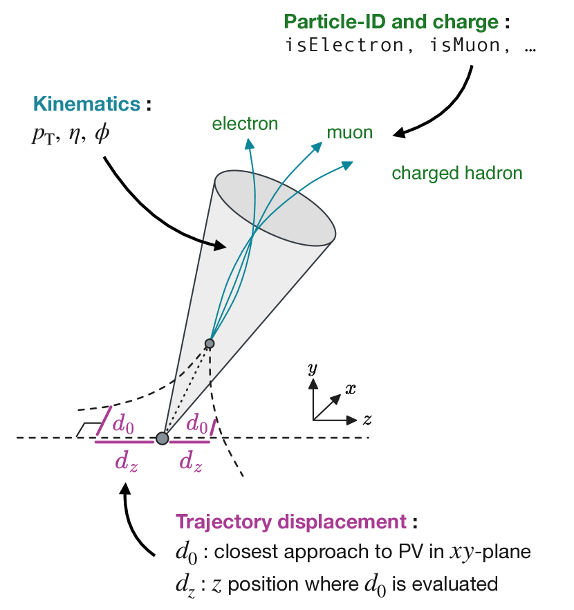
Figure 1: Schematic overview of the different jet constituent features available in the JetClass dataset. The horizontal line at the bottom represents the beam axis and the circle on this line represents the primary vertex (PV).

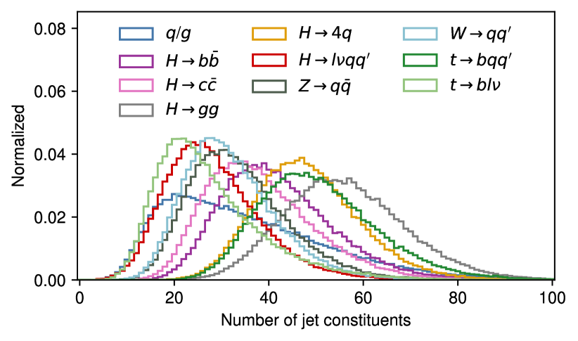
(a)

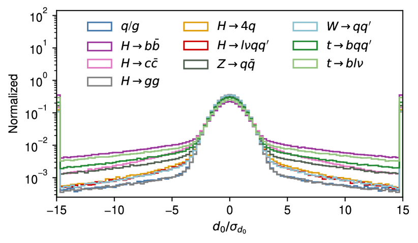
(b)

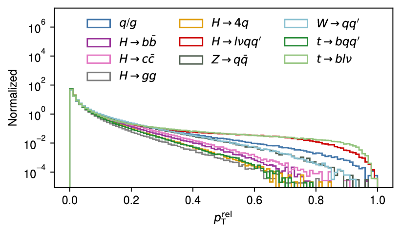
(c)

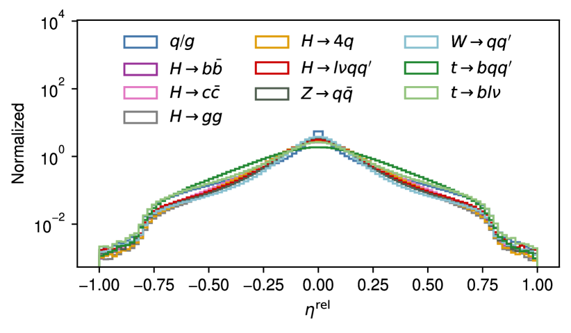
(d)

Figure 2: Overview of some of the features from the JetClass dataset: (a) shows the number of jet constituents, (b) shows the significance of the transverse impact parameter $d_{0}$, (c) shows the fraction of the jet $p_{\text{T}}$ carried by the jet constituent and (d) shows the difference $\eta^{\text{rel}}$ between the constituent pseudorapidity and the jet axis. The impact parameter significance $d_{0}/\sigma_{d_{0}}$ is only shown for charged particles since the impact parameter is 0 for neutral particles. The number of jet constituents is a jet-level feature our model is conditioned on while the remaining features correspond to constituent-level features that our model generates.

So far, efforts for jet generation have focused almost exclusively on the JetNet dataset of Refs. [38, 39]. Originally generated by [40], this dataset was subsequently adopted in the works of Ref. [5] as a benchmark dataset for jet generative modeling. However, the JetNet dataset has a number of drawbacks that are readily becoming apparent. First, its limited size (180k jets per jet type) means there are not enough jets in JetNet to facilitate the training of state-of-the-art generative models as well as metrics such as the binary classifier metric [41, 42] which require additional training data. Second, JetNet uses small-radius ($R=0.4$) jets (although the description in [5] incorrectly states a cone-size of $R=0.8$ which is in disagreement with the observed angular distribution of constituents). This can lead to decay products not being fully contained in the jet, which can be seen e.g. in distributions such as the jet mass for top quarks, where there is a prominent secondary mass peak. Finally, JetNet focuses solely on the kinematics of the jet constituents, whereas there is a wealth of additional information inside the jets that could also be modeled, such as trajectory displacement, charge, and particle ID as illustrated in Figure 1.

In this work, we introduce the first generative model for jet constituents trained on the larger and more substantial JetClass dataset [43]. Other than demonstrating that existing techniques scale well to this new dataset, we also tackle new challenges introduced by the JetClass dataset, including the additional features mentioned above. We show that a single architecture consisting of a continuous normalizing flow (CNF)  [44] constructed out of EPiC layers and trained with the flow matching technique [21, 22, 23, 24] can learn to model all ten jet types and all features of JetClass well, both kinematics and beyond. Using the much larger statistics provided by JetClass  we also train binary classifier metrics on the generative model for the first time, which allows us to further evaluate our results.

The rest of this paper is structured as follows:  Section II describes the JetClass dataset in more detail;  Section III introduces the used generative model; Section IV provides an overview of the generative performance; and finally Section V concludes this work.

II Dataset

We use the JetClass dataset [43], originally introduced in Ref. [45]. This dataset encompasses various features both on jet level and on jet constituent level for ten different types of jets initiated by gluons and quarks ($q/g$), top quarks ($t$), as well as $W$, $Z$, and $H$ bosons. Jets initiated by a top quark or a Higgs boson are further categorized based on their different decay channels, resulting in the following ten categories: $q/g$, $t\to bqq^{\prime}$, $t\to b\ell\nu$, $Z\to q\bar{q}$, $W\to qq^{\prime}$, $H\to b\bar{b}$, $H\to c\bar{c}$, $H\to gg$, $H\to 4q$, and $H\to\ell\nu qq^{\prime}$.

Table 1: Features used for the studies in this paper. All features are either taken directly from the JetClass dataset or calculated from existing entries in the JetClass dataset. The model is conditioned on the jet features (first block) during generation. The remaining features are the constituent features our model is trained to generate.

Category	Variable	Definition
	Jet type	Indicating the type of the jet (i.e. $t\to bqq^{\prime}$, $q/g$, …)
Jet features	$n_{\mathrm{const}}$	Number of constituents in the jet
	$p_{\mathrm{T}}^{\mathrm{jet}}$	Transverse momentum of the jet
	$\eta^{\mathrm{jet}}$	Pseudorapidity of the jet
	$\eta^{\text{rel}}$	Difference in pseudorapidity $\eta$ between the constituent and the jet axis
Kinematics	$\phi^{\text{rel}}$	Difference in azimuthal angle $\phi$ between the constituent and the jet axis
	$p_{\mathrm{T}}^{\text{rel}}$	Fraction of the constituent $p_{\text{T}}$ and the jet $p_{\text{T}}$
	$d_{0}$	Transverse impact parameter value
Trajectory	$d_{z}$	Longitudinal impact parameter value
displacement	$\sigma_{d_{0}}$	Error of measured transverse impact parameter
	$\sigma_{d_{z}}$	Error of measured longitudinal impact parameter
	charge	Electric charge of the particle
	isChargedHadron	Flag if the particle is a charged hadron (|pid|==211 or 321 or 2212)
Particle	isNeutralHadron	Flag if the particle is a neutral hadron (|pid|==130 or 2112 or 0)
identification	isPhoton	Flag if the particle is a photon (pid==22)
	isElectron	Flag if the particle is an electron (|pid|==11)
	isMuon	Flag if the particle is a muon (|pid|==13)

The jets are extracted from simulated events that are generated with MadGraph5_aMC@NLO [46]. Parton showering and hadronization is performed with Pythia [1] and detector effects are simulated with Delphes [47] using the CMS detector [48] card. The jets are clustered with the anti-$k_{\mathrm{T}}$ algorithm [49] with a jet radius of $R=0.8$. Jets are required to have a transverse momentum of $$500\text{\,}\mathrm{G}\mathrm{e}\mathrm{V}$<p_{\mathrm{T}}^{\mathrm{jet}}<$1000\text{\,}\mathrm{G}\mathrm{e}\mathrm{V}$$ and a pseudorapidity of $|\eta^{\mathrm{jet}}|<2$. Furthermore, for all jets, except for the $q/g$ jets, only those that contain all decay products of the boson or top quark are considered in the dataset.

Representative distributions of some of the features available in the JetClass dataset are presented in Figure 2, illustrating substantial distinctions among the various jet categories. As can be seen in 2(a), the dataset covers jet types with a large variety of number of jet constituents. Additionally, 2(b) illustrates the expected tails of varying extents in the trajectory displacement. Notably, jet categories that do not include $b$ quarks or $c$ quarks have a rather narrow peak around 0, while jet categories that do include those types of quarks have a more spread out distribution, corresponding to the long lifetime of $b$- and $c$-hadrons.

The features that are used by our model are listed with the corresponding definitions in Table 1. By conditioning our model on the jet type, we can train one model that is capable of generating all ten jet types. Furthermore, the jet transverse momentum $p_{\mathrm{T}}^{\mathrm{jet}}$ and the jet pseudorapidity $\eta^{\mathrm{jet}}$ are used as conditioning features in order to be able to obtain the non-relative constituent-level features after jet generation.

The kinematic features of the jet constituents are measured relative to the jet axis. i.e.

$$\eta^{\mathrm{rel}} =\eta^{\mathrm{const}}-\eta^{\mathrm{jet}}$$ (1)

$$\phi^{\mathrm{rel}} =\phi^{\mathrm{const}}-\phi^{\mathrm{jet}}$$ (2)

$$p_{\mathrm{T}}^{\mathrm{rel}} =p_{\mathrm{T}}^{\mathrm{const}}/p_{\mathrm{T}}^{\mathrm{jet}}\,.$$ (3)

The trajectory displacement features as well as the discrete particle identification features are taken directly from the JetClass dataset. The jet constituents are assumed to be massless, as we do not include the particle energy in our model. In total, our model thus utilizes 13 constituent features to comprehensively characterize the constituents within generated jets. This set of features represents all available constituent features, from the JetClass dataset, with the only exception being the constituent energy.

III Model

Overall, we follow the recent flow matching paradigm [21, 22, 23, 24], using Gaussian probability paths as explained in Ref. [14].

The architecture of our model is based on the EPiC-FM model which was introduced in Ref. [14] with a few adjustments. It uses EPiC layers [7] to transform jet constituents as point clouds while preserving permutation symmetry. Besides the point cloud, EPiC layers also take as input a global context vector, which learns to encode higher-level information about the whole point cloud by using both mean and sum aggregation over the points. The use of the global context vector is responsible for the computational efficiency of the EPiC layers – unlike the quadratic scaling for architectures that include edge features between all pairs of points (such as transformers), the computational cost of EPiC layers only scales linearly with the number of points.

A full list of the specific hyperparameters of the model is summarized in the Appendix in Table 5. While the overall architecture is based on Ref. [14], it is scaled up for the JetClass dataset, with 20 EPiC layers instead of 6, an embedding dimension of 300 instead of 128, and a 16-dimensional global vector.

The jet-type conditioning is realized with a one-hot encoding, while the jet transverse momentum $p_{\mathrm{T}}^{\mathrm{jet}}$ and jet pseudorapidity $\eta^{\mathrm{jet}}$ are used without any preprocessing. For jet generation, we fit a kernel density estimator (KDE) to the jet features ($p_{\mathrm{T}}^{\mathrm{jet}}$, $\eta^{\mathrm{jet}}$, and $n_{\mathrm{const}}$) for each jet type individually, and sample from the KDE to obtain the conditioning features and the number of constituents for the generated jets. For each jet, our model acts on a tensor of shape $(N,C)$, with $N=128$ being the maximum number of jet constituents and $C$ being the number of constituent features. To generate jets with fewer constituents ($n_{\mathrm{const}}<128$), we apply a binary mask throughout training; this ensures that the inputs and outputs of the EPiC layers are valid and in particular guarantees that the mean and sum aggregation steps within the EPiC layers are correctly normalized. The particle features are shifted to mean 0 and scaled to the same standard deviation. Furthermore, only particles with $|\eta^{\text{rel}}|<1$ are considered to remove a few particles in the tails of this distribution.

The model is trained for 500 epochs with a training sample size of 3M jets ($300\,000$ jets per jet type).

The AdamW optimizer [50] is used with a maximum learning rate of 0.001 and weight decay of $5\text{\times}{10}^{-5}$. The learning rate is scheduled with a cosine-annealing learning rate scheduler with a linear warm-up period over 20 epochs. The model after the last epoch is chosen for evaluation. For the jet generation, we use the midpoint ODE solver, a 2^nd order Runge-Kutta variant. After jet generation, the $p_{\mathrm{T}}^{\text{rel}}$ values of the generated jet constituents are clipped to the minimum and maximum values that are found in the training dataset. Furthermore, the electric charge is rounded to the nearest integer within {-1, 0, 1}. The remaining discrete particle-identification features are post-processed with an argmax operation such that the particle-ID feature with the maximum value is set to 1 and the remaining ones are set to 0. This ensures that generated particles are unambiguously assigned to one particle type. It should be noted that this might not be the ideal handling of such discrete features, which could be improved and further investigated in future work. The model is implemented in PyTorch [51] using PyTorch Lightning [52].

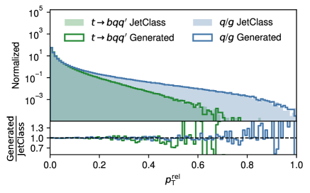
(a)

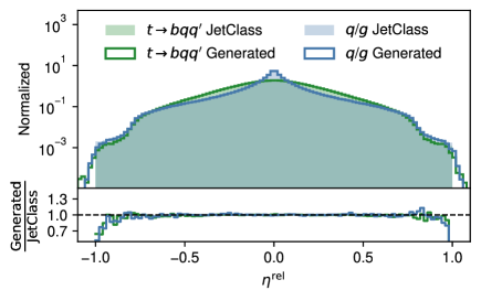
(b)

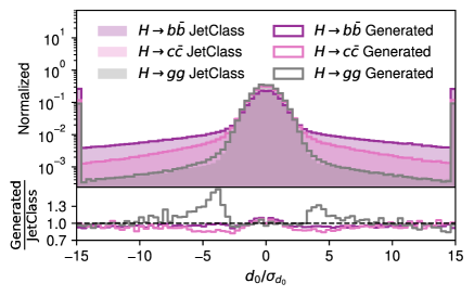
(c)

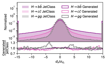
(d)

Figure 3: Two kinematic features and the trajectory displacement of the jet constituents as generated by our model (solid lines) in comparison to the distributions obtained from the JetClass dataset (semi-transparent histograms). The upper row shows (a) the relative transverse momentum and (b) the relative pseudorapidity. The lower row shows (c) the transverse impact parameter significance and (d) the longitudinal impact parameter significance. Only charged particles are shown in the histograms of the trajectory displacement and the outermost bins show the underflow and overflow bins.

Table 2: Kullback-Leibler divergence of constituent-level features with respect to the JetClass dataset.

	$\mathrm{KL}^{p_{\mathrm{T}}^{\mathrm{rel}}}~{}(\times 10^{-3})$	$\mathrm{KL}^{\eta^{\mathrm{rel}}}~{}(\times 10^{-3})$	$\mathrm{KL}^{\phi^{\mathrm{rel}}}~{}(\times 10^{-3})$	$\mathrm{KL}^{d_{0}/\sigma_{d_{0}}}~{}(\times 10^{-3})$	$\mathrm{KL}^{d_{z}/\sigma_{d_{z}}}~{}(\times 10^{-3})$
Truth ($q/g$)	$0.059\,61\pm 0.010\,34$	$0.080\,30\pm 0.009\,62$	$0.072\,17\pm 0.010\,02$	$0.133\,01\pm 0.014\,22$	$0.112\,29\pm 0.015\,00$
EPiC-FM ($q/g$)	$0.073\,07\pm 0.007\,07$	$0.130\,12\pm 0.021\,64$	$0.118\,79\pm 0.011\,54$	$2.203\,54\pm 0.061\,86$	$3.717\,44\pm 0.087\,03$
Truth ($H\to b\bar{b}$)	$0.048\,09\pm 0.003\,93$	$0.074\,78\pm 0.012\,12$	$0.060\,23\pm 0.008\,22$	$0.102\,21\pm 0.010\,20$	$0.091\,93\pm 0.010\,75$
EPiC-FM ($H\to b\bar{b}$)	$0.070\,50\pm 0.008\,39$	$0.121\,90\pm 0.022\,42$	$0.116\,84\pm 0.022\,37$	$2.644\,17\pm 0.086\,23$	$1.473\,73\pm 0.071\,94$
Truth ($H\to c\bar{c}$)	$0.054\,12\pm 0.007\,06$	$0.074\,86\pm 0.013\,76$	$0.084\,56\pm 0.015\,10$	$0.106\,01\pm 0.019\,20$	$0.105\,72\pm 0.024\,10$
EPiC-FM ($H\to c\bar{c}$)	$0.077\,61\pm 0.006\,80$	$0.113\,33\pm 0.019\,60$	$0.134\,39\pm 0.008\,82$	$2.782\,66\pm 0.101\,72$	$1.963\,64\pm 0.077\,82$
Truth ($H\to gg$)	$0.034\,37\pm 0.002\,46$	$0.057\,83\pm 0.015\,55$	$0.052\,71\pm 0.008\,18$	$0.074\,57\pm 0.013\,71$	$0.070\,54\pm 0.009\,79$
EPiC-FM ($H\to gg$)	$0.056\,76\pm 0.008\,97$	$0.101\,10\pm 0.013\,66$	$0.101\,04\pm 0.014\,11$	$2.332\,04\pm 0.095\,48$	$3.529\,88\pm 0.123\,78$
Truth ($H\to 4q$)	$0.039\,49\pm 0.004\,68$	$0.057\,03\pm 0.007\,17$	$0.053\,21\pm 0.010\,81$	$0.080\,44\pm 0.011\,37$	$0.079\,61\pm 0.018\,84$
EPiC-FM ($H\to 4q$)	$0.056\,84\pm 0.006\,25$	$0.118\,38\pm 0.019\,92$	$0.106\,26\pm 0.015\,25$	$2.257\,38\pm 0.069\,70$	$3.212\,07\pm 0.119\,66$
Truth ($H\to\ell\nu qq^{\prime}$)	$0.071\,17\pm 0.012\,95$	$0.098\,79\pm 0.023\,04$	$0.096\,90\pm 0.014\,43$	$0.139\,60\pm 0.011\,04$	$0.133\,31\pm 0.016\,25$
EPiC-FM ($H\to\ell\nu qq^{\prime}$)	$0.103\,07\pm 0.013\,51$	$0.154\,97\pm 0.022\,99$	$0.137\,35\pm 0.008\,45$	$2.106\,21\pm 0.075\,97$	$2.605\,66\pm 0.090\,77$
Truth ($Z\to q\bar{q}$)	$0.061\,02\pm 0.008\,18$	$0.076\,89\pm 0.011\,91$	$0.077\,31\pm 0.013\,03$	$0.138\,42\pm 0.032\,11$	$0.127\,84\pm 0.012\,33$
EPiC-FM ($Z\to q\bar{q}$)	$0.073\,58\pm 0.009\,82$	$0.145\,04\pm 0.024\,54$	$0.126\,48\pm 0.018\,55$	$3.250\,17\pm 0.161\,54$	$2.110\,03\pm 0.128\,06$
Truth ($W\to qq^{\prime}$)	$0.062\,80\pm 0.010\,86$	$0.088\,04\pm 0.009\,49$	$0.086\,40\pm 0.008\,44$	$0.123\,65\pm 0.014\,53$	$0.126\,13\pm 0.018\,49$
EPiC-FM ($W\to qq^{\prime}$)	$0.082\,44\pm 0.007\,68$	$0.140\,93\pm 0.022\,78$	$0.130\,22\pm 0.016\,62$	$2.176\,27\pm 0.048\,47$	$2.592\,12\pm 0.110\,57$
Truth ($t\to bqq^{\prime}$)	$0.042\,58\pm 0.006\,68$	$0.059\,73\pm 0.004\,92$	$0.057\,13\pm 0.007\,47$	$0.079\,89\pm 0.010\,25$	$0.079\,61\pm 0.010\,68$
EPiC-FM ($t\to bqq^{\prime}$)	$0.082\,08\pm 0.011\,03$	$0.088\,61\pm 0.013\,56$	$0.099\,72\pm 0.010\,65$	$1.793\,05\pm 0.065\,39$	$1.789\,30\pm 0.095\,54$
Truth ($t\to b\ell\nu$)	$0.072\,31\pm 0.014\,01$	$0.126\,61\pm 0.018\,24$	$0.148\,66\pm 0.033\,35$	$0.149\,49\pm 0.015\,00$	$0.152\,13\pm 0.019\,52$
EPiC-FM ($t\to b\ell\nu$)	$0.106\,28\pm 0.016\,14$	$0.196\,89\pm 0.033\,51$	$0.185\,01\pm 0.057\,09$	$1.761\,65\pm 0.087\,47$	$1.459\,49\pm 0.062\,27$

IV Results

In the following, we first evaluate the distributions of the constituent-level features that the model was trained on. Afterwards, we evaluate jet-level features that are derived from the constituent-level features, namely the jet mass, the $N$-subjettiness [53] ratios $\tau_{32}$ and $\tau_{21}$ as well as the $D_{2}$ [54] observable, which is a ratio of energy correlation functions [55]. Lastly, we train a binary classifier as in Ref. [41] to distinguish between real jets from the JetClass dataset and fake jets generated by our model, which allows us to evaluate the quality of the generated jets further.

For the evaluation of our model, we generate 5M jets (i.e. $500\,000$ jets per jet type) and evaluate the different feature categories separately. Instead of using the Wasserstein-1 distance as a metric for the agreement between the generated and the target distribution as in [5, 7, 8], we are following [14] and using the Kullback-Leibler (KL) divergence. As explained there, this metric choice is motivated by the fact that the Wasserstein-1 distance is well-suited for detecting distributions with different support, but can lead to misleading results for cases where the distributions have the same overlapping support but differ mainly in their shapes.

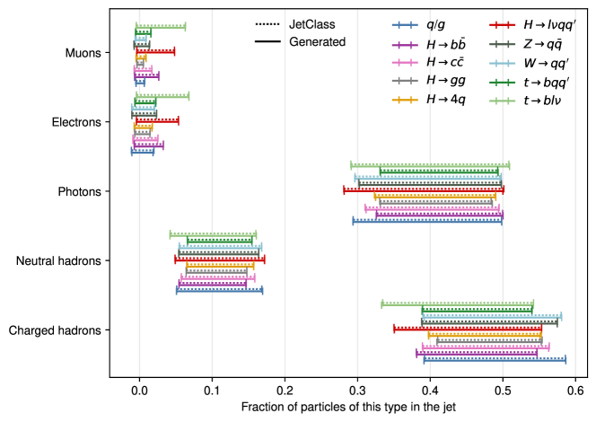
Figure 4: Average fraction of jet constituents of different particle types. For each jet type, the intervals show the mean value over all evaluated jets with up and down variations of one standard deviation. The dotted lines show the values obtained for real jets from the JetClass dataset and the solid lines show the values obtained for the generated jets.

The KL divergence values are calculated by splitting the generated jets and the JetClass jets into 10 batches of $50\,000$ jets each and then calculate the reverse KL divergence for each batch. This allows us to evaluate the uncertainty of the KL divergence to be able to quantitatively compare it to the truth distribution. The reported values are the mean of those 10 individual KL divergence values and their standard deviation. For the truth values of the KL divergence, we take two independent samples of the test dataset and then calculate the KL divergence between those two samples using the same procedure as when comparing the real and generated jets. The bin edges of the binned probability distributions are constructed by calculating 100 equiprobable quantiles from the target distribution and setting the edges of the outermost bins to the minimum and maximum values found in the target distribution. Outliers of the distribution from the generated jets are put into the first and last bin.

IV.1 Jet constituent modeling

A comparison of the kinematic features of the jet constituents is shown in Figure 3. For this comparison, we chose to compare $t\to bqq^{\prime}$ jets and $q/g$ jets, since those two types of jets have distinct characteristics in both the $\eta^{\text{rel}}$ and the $p_{\mathrm{T}}^{\text{rel}}$ distribution. While particles in $t\to bqq^{\prime}$ jets have on average a larger $\eta^{\text{rel}}$ and thus have an overall wider $\eta^{\text{rel}}$ distribution, $q/g$ jets are more collimated, resulting in a sharper $\eta^{\text{rel}}$ peak around $\eta^{\mathrm{rel}}=0$. Concerning the $p_{\mathrm{T}}^{\text{rel}}$ distribution, $t\to bqq^{\prime}$ jets are expected to show a smaller tail towards larger $p_{\mathrm{T}}^{\text{rel}}$ values, since $t\to bqq^{\prime}$ jets contain on average more constituents and thus the jet $p_{\text{T}}$ is distributed over more particles, leading to smaller $p_{\mathrm{T}}^{\text{rel}}$ values. The generated distributions of all three kinematic features agree very well with the corresponding distribution from the JetClass dataset, showing that our model is capable of generating jets of very different kinematic properties. This is also confirmed by the KL divergence values listed in Table 2, which only have a small deviation from the truth values.

A comparison of the trajectory displacement modeling is shown in Figure 3 for $H\to b\bar{b}$, $H\to c\bar{c}$ and $H\to gg$ jets. Due to the long lifetime of $b$- and $c$-hadrons, the trajectory displacement of jet constituents associated with those hadrons is expected to be on average larger than for other jet constituents. Thus, the trajectory displacement distributions of $H\to b\bar{b}$ and $H\to c\bar{c}$ jets are expected to be wider than the trajectory displacement distribution of $H\to gg$ jets. Since the trajectory displacement is by definition zero for neutral particles in the JetClass dataset, only charged particles are considered in the histograms in Figure 3. For all three jet types, the histograms of the generated jets agree very well with the histograms of the real jets, showing that our model is capable of correctly modeling the trajectory displacement of the jet constituents. Notably, our model is able to catch the essential differences between the trajectory displacement distributions of $H\to b\bar{b}$, $H\to c\bar{c}$ and $H\to gg$ jets, which is an important feature from the physics point of view. However, as seen both in the ratio panels in Figure 3 and in the corresponding KL divergence values in Table 2, the agreement between the target distribution and the distribution obtained from the generated jets is worse for the impact parameter features than for the kinematic features, showing that the modeling of these distributions is more challenging. This could be further optimized in future work by choosing a different preprocessing for the impact parameter features, by e.g. transforming them using the hyperbolic tangent function, which would remove the large tails of the distributions.

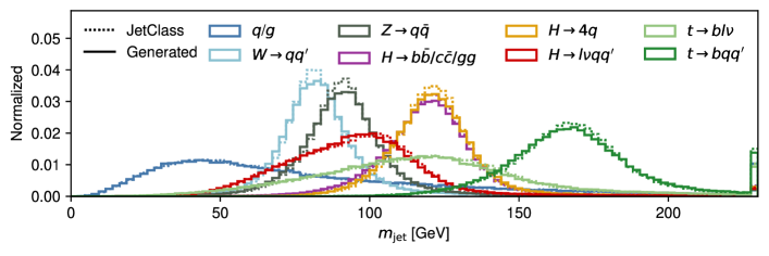
(a)

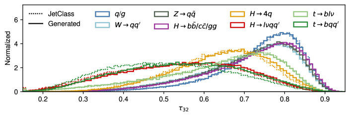
(b)

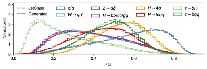
(c)

Figure 5: Jet mass (a) and subjettiness ratios $\tau_{32}$ (b) and $\tau_{21}$ (c) for all ten jet types. The histograms in dotted lines show the distributions obtained from the JetClass dataset (i.e. real jets) and the solid lines show the histograms obtained from the generated jets. Jets from the categories $H\to b\bar{b}$, $H\to c\bar{c}$ and $H\to gg$ are grouped into one joint histogram for better readability, since the individual histograms show very similar shapes.

Table 3: Kullback-Leibler divergence of jet-level observables with respect to the JetClass dataset.

	$\mathrm{KL}^{m_{\mathrm{jet}}}~{}(\times 10^{-3})$	$\mathrm{KL}^{\tau_{21}}~{}(\times 10^{-3})$	$\mathrm{KL}^{\tau_{32}}~{}(\times 10^{-3})$	$\mathrm{KL}^{D_{2}}~{}(\times 10^{-3})$
Truth ($q/g$)	$1.953\,55\pm 0.218\,44$	$1.915\,73\pm 0.262\,76$	$2.005\,00\pm 0.278\,46$	$1.915\,99\pm 0.401\,18$
EPiC-FM ($q/g$)	$2.017\,35\pm 0.323\,38$	$4.281\,62\pm 0.454\,04$	$2.274\,48\pm 0.243\,69$	$4.680\,22\pm 0.439\,16$
Truth ($H\to b\bar{b}$)	$1.929\,57\pm 0.220\,09$	$1.950\,41\pm 0.209\,32$	$2.070\,44\pm 0.225\,14$	$1.967\,65\pm 0.218\,95$
EPiC-FM ($H\to b\bar{b}$)	$3.250\,42\pm 0.464\,53$	$3.616\,70\pm 0.576\,11$	$2.704\,61\pm 0.356\,94$	$3.317\,23\pm 0.521\,72$
Truth ($H\to c\bar{c}$)	$2.030\,55\pm 0.310\,76$	$1.999\,80\pm 0.231\,85$	$2.167\,72\pm 0.335\,99$	$1.904\,92\pm 0.180\,12$
EPiC-FM ($H\to c\bar{c}$)	$4.801\,21\pm 0.463\,92$	$6.425\,21\pm 0.613\,45$	$3.082\,88\pm 0.491\,70$	$3.741\,88\pm 0.475\,70$
Truth ($H\to gg$)	$1.970\,78\pm 0.184\,03$	$1.833\,53\pm 0.256\,61$	$1.875\,86\pm 0.224\,39$	$1.969\,64\pm 0.180\,47$
EPiC-FM ($H\to gg$)	$3.781\,46\pm 0.413\,47$	$3.813\,34\pm 0.594\,99$	$2.736\,55\pm 0.421\,33$	$3.219\,85\pm 0.507\,20$
Truth ($H\to 4q$)	$2.212\,78\pm 0.360\,37$	$2.086\,35\pm 0.300\,42$	$1.996\,70\pm 0.265\,42$	$1.860\,75\pm 0.306\,99$
EPiC-FM ($H\to 4q$)	$5.226\,04\pm 0.488\,94$	$5.079\,49\pm 0.491\,46$	$7.842\,62\pm 0.702\,45$	$3.231\,33\pm 0.463\,96$
Truth ($H\to\ell\nu qq^{\prime}$)	$1.889\,46\pm 0.312\,49$	$1.927\,82\pm 0.266\,29$	$2.035\,32\pm 0.233\,79$	$1.989\,39\pm 0.207\,44$
EPiC-FM ($H\to\ell\nu qq^{\prime}$)	$3.482\,86\pm 0.487\,94$	$3.483\,49\pm 0.451\,68$	$9.123\,05\pm 0.866\,10$	$2.312\,72\pm 0.321\,74$
Truth ($Z\to q\bar{q}$)	$2.056\,68\pm 0.180\,41$	$1.984\,99\pm 0.322\,02$	$1.948\,63\pm 0.238\,01$	$2.044\,05\pm 0.200\,46$
EPiC-FM ($Z\to q\bar{q}$)	$4.835\,33\pm 0.548\,34$	$3.507\,61\pm 0.453\,51$	$1.963\,15\pm 0.213\,06$	$2.431\,36\pm 0.247\,72$
Truth ($W\to qq^{\prime}$)	$2.051\,19\pm 0.394\,46$	$2.037\,59\pm 0.217\,66$	$2.036\,98\pm 0.193\,67$	$1.991\,16\pm 0.244\,29$
EPiC-FM ($W\to qq^{\prime}$)	$5.825\,06\pm 0.466\,22$	$4.243\,35\pm 0.635\,11$	$2.631\,88\pm 0.404\,72$	$3.122\,18\pm 0.493\,96$
Truth ($t\to bqq^{\prime}$)	$1.860\,03\pm 0.248\,93$	$1.998\,56\pm 0.261\,65$	$2.059\,73\pm 0.235\,60$	$1.936\,81\pm 0.308\,60$
EPiC-FM ($t\to bqq^{\prime}$)	$4.668\,58\pm 0.610\,07$	$7.873\,70\pm 0.859\,60$	$29.864\,26\pm 1.039\,10$	$2.952\,29\pm 0.431\,81$
Truth ($t\to b\ell\nu$)	$2.001\,15\pm 0.142\,16$	$1.850\,14\pm 0.221\,96$	$1.975\,56\pm 0.211\,40$	$1.995\,06\pm 0.273\,39$
EPiC-FM ($t\to b\ell\nu$)	$3.368\,23\pm 0.226\,94$	$5.812\,81\pm 0.536\,40$	$2.573\,32\pm 0.372\,77$	$3.775\,54\pm 0.467\,62$

The evaluation of the particle-ID modeling is shown in Figure 4, where we show the average fraction of jet constituents of different particle types for all ten jet types. For each jet type, the intervals show the mean value over all evaluated jets with up and down variation of one standard deviation. The agreement between the generated jets and the real jets is very good for all jet types, showing that on average the generated jets contain the same fraction of different particle types as the real jets. The modeling of the electric charge also shows very good agreement, which is shown in the Appendix in Appendix A.

Table 4: AUC scores of the classifier test for the ten different jet types.

Jet type	AUC score
$q/g$	$0.681$
$W\to qq^{\prime}$	$0.683$
$Z\to q\bar{q}$	$0.689$
$H\to\ell\nu qq^{\prime}$	$0.706$
$t\to b\ell\nu$	$0.706$
$H\to b\bar{b}$	$0.712$
$H\to gg$	$0.716$
$H\to c\bar{c}$	$0.728$
$H\to 4q$	$0.809$
$t\to bqq^{\prime}$	$0.829$

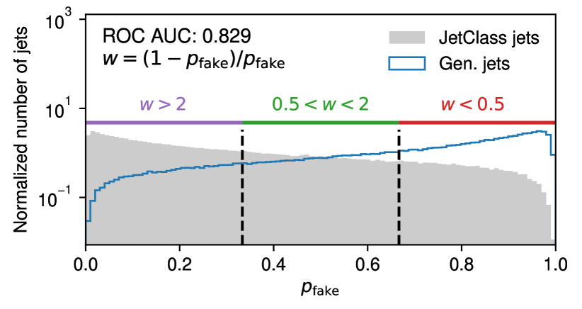
(a)

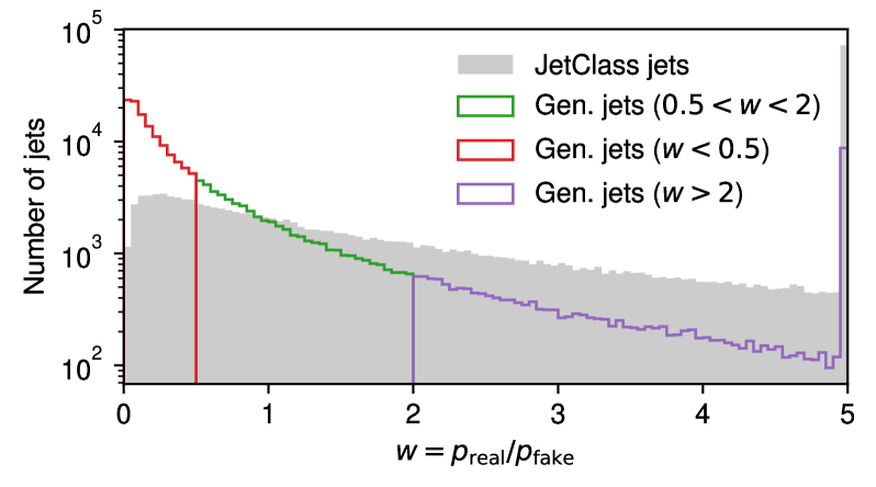
(b)

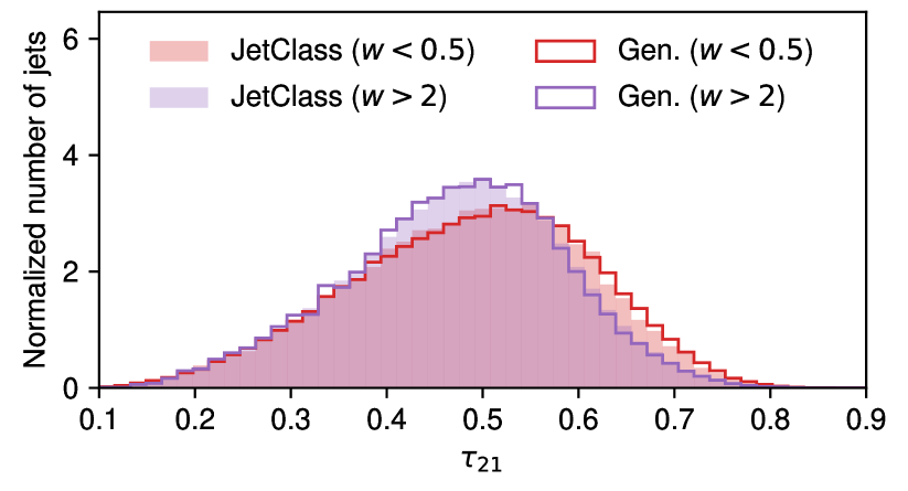
(c)

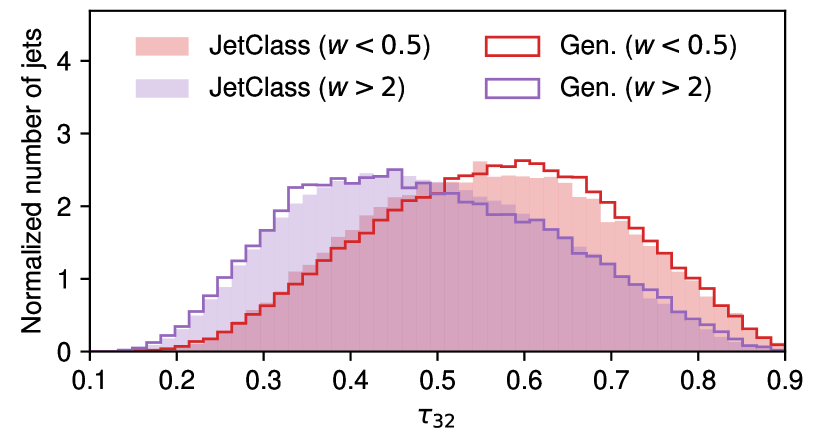
(d)

Figure 6: Results of the classifier test for $t\to bqq^{\prime}$ jets. Figure (a) shows the classifier output for real and fake jets, as well as the cut values for the three regions. Figure (b) shows the weight distribution of the fake jets with differently colored histograms for the fake jets from the different regions. Figures (c) and (d) show the $\tau_{21}$ and $\tau_{32}$ distributions for the real jets and the fake jets from the regions where the classifier output distribution is dominated by real jets or fake jets.

IV.2 Jet substructure modeling

The jet mass $m_{\mathrm{jet}}$ and the two subjettiness ratios $\tau_{32}$ and $\tau_{21}$ are shown in Figure 5 for the different jet types. The real jets are shown in dotted lines while the generated jets are shown in solid lines. Both the jet mass and the subjettiness ratio distributions show very good agreement for all jet types. The largest deviations between the target distribution and the distribution of the generated jets are seen for $t\to bqq^{\prime}$ and $H\to\ell\nu qq^{\prime}$, where the distribution of the generated jets peaks at a larger value of $\tau_{32}$. This mismodeling also shows in the values of the KL divergence which are listed in Table 3 for some of the jet-level observables. Further studies were done to determine whether narrowing down our model’s features to just kinematics and whether training solely on $t\to bqq^{\prime}$ jets enhances the modeling of the $t\to bqq^{\prime}$ substructure, which can be found in the Appendix in Appendix C.

IV.3 Classifier test

In addition to the evaluation presented in the previous subsections, we also investigate the performance of our model with the classifier test proposed in Ref. [41]. Thus, a binary classifier is trained to distinguish between real jets from the JetClass dataset and fake jets that were generated with our model. This classifier test is performed for each jet type separately.

To train the classifier, we use the 500k fake jets and 500k real jets from the previous evaluation, and split them into 250k, 50k and 200k jets for training, validation and testing of the classifier, respectively. The classifier is trained by fine-tuning the ParT-kin version from Ref. [45], which means that the last MLP of the ParT architecture is re-initialized and changed to two output nodes. The classifier is then trained with real vs fake jets using the AdamW optimizer [50] with a learning rate of 0.001 for a few epochs. However, it should be noted that the classifier training was not extensively optimized. We noticed that the validation loss converges after just a few epochs after which the classifier starts to overfit. We therefore chose to use the model with the highest validation accuracy before clear signs of overfitting are visible.

The AUC values of the corresponding ROC curves are shown in Table 4. To estimate the uncertainty of the classifier scores, five classifiers are trained for $H\to b\bar{b}$ jets with different random seeds. All classifiers converge at similar performance, with the standard deviation of the AUC scores being $\sigma_{\mathrm{AUC}}(H\to b\bar{b})=$0.003$$.

The largest AUC value is obtained for $t\to bqq^{\prime}$ jets with an AUC of $0.829$, confirming again that this is the most challenging jet type for our model. The results of the corresponding classifier test are shown in Figure 6 in more detail. However, the AUC value for $t\to bqq^{\prime}$ jets is still well below 1, allowing us to investigate the $t\to bqq^{\prime}$ jets corresponding to different regions of the classifier output. Therefore, following Ref. [42], we split the $t\to bqq^{\prime}$ jets into three regions, based on their weight $w=p_{\mathrm{real}}/p_{\mathrm{fake}}$ as illustrated in 6(a) and 6(b). The first region contains jets with $w>2$, the second region contains jets with $0.5<w<2$, and the third region contains jets with $w<0.5$. Thus, the outer regions correspond to jets that are clearly identified as either real or fake jets, while the center region contains jets where the classifier is not able to clearly distinguish them.

The corresponding subjettiness ratios $\tau_{21}$ and $\tau_{32}$ are shown in 6(c) and 6(d) for $t\to bqq^{\prime}$ jets from the outer regions. This shows the jet substructure differences between the $t\to bqq^{\prime}$ jets that are clearly classified as either real or fake. $t\to bqq^{\prime}$ jets that correspond to $w>2$, i.e. jets of which the classifier is rather certain that they are real jets, have on average a smaller $\tau_{32}$ value than $t\to bqq^{\prime}$ jets that are clearly identified as fake jets ($w<0.5$). Therefore, the classifier classifies $t\to bqq^{\prime}$ jets that are more 3-prong-like (i.e. with a smaller $\tau_{32}$ value) as real $t\to bqq^{\prime}$ jets, while $t\to bqq^{\prime}$ jets that are less 3-prong-like (i.e. with a larger $\tau_{32}$ value) tend to be classified as fake $t\to bqq^{\prime}$ jets. Thus, our model seems to struggle with the modeling of the 3-prong structure of $t\to bqq^{\prime}$ jets, which is also consistent with the results from the previous sections, where we saw that the $\tau_{32}$ distribution of the generated $t\to bqq^{\prime}$ jets peaks at a slightly larger value than the $\tau_{32}$ distribution of the real $t\to bqq^{\prime}$ jets. The peak at the larger $\tau_{32}$ value and thus the overall shift of the distribution is caused by the poorly modeled jets: given that $61\text{\,}\mathrm{\char 37\relax}$ of the fake $t\to bqq^{\prime}$ jets have $w<0.5$, the overall $\tau_{32}$ distribution of the fake jets is dominated by jets with larger $\tau_{32}$. On the other hand, only $15\text{\,}\mathrm{\char 37\relax}$ of the real $t\to bqq^{\prime}$ jets have $w<0.5$, and $58\text{\,}\mathrm{\char 37\relax}$ of the real $t\to bqq^{\prime}$ jets have $w>2$, which correspond to the purple distribution in 6(d).

V Conclusion

Generative surrogate models of different physical processes are a powerful new tool with multiple potential applications. So far, speeding up classical simulations, either of particle interactions in calorimeters or of the calculation of matrix elements, has been the primary focus of research. However, learning surrogate models of jets has its own interesting aspects: i) such models can, in principle, be trained on collider data, allowing the interpolation of distributions to estimate backgrounds; ii) they can form parts of a fully differentiable analysis and interpretation chain; iii) an interpretable version trained directly on collider data may provide an additional way of gaining insight into showering and hadronization processes; iv) learning jets at the constituent level is a crucial stepping stone to simulating full events at the finest granularity; and v) they provide a meaningful testbed to benchmark progress in generative models for point clouds.

The main result of this work is that the EPiC-FM [14] framework can be easily scaled up to more complex datasets. The move from the JetNet to the JetClass dataset results in more classes (10 instead of 5), more features per jet (13 instead of 3), geometrically larger jets ($R=0.8$ instead of $R=0.4$), and finally more jets available for training with JetClass containing a factor of 70 more jets per jet type than JetNet.

Overall we observe an accurate description of physical quantities. For some individual features and classes, the agreement between generated data and ground truth is on the same level as the statistical fluctuations between different samples drawn from the ground truth distribution. In general, more complex final states (i.e. multi-pronged signals with intermediate resonances) are more difficult to describe than relatively simple light quark or gluon-induced jets.

The capability to model quantities beyond jet kinematics demonstrated here will serve as an important factor in further increasing the performance of anomaly detection algorithms. Previous results already showed that going from a few high-level to many low-level features increases the maximum achievable significance improvement by more than a factor of three [4]. Access to trajectory displacement and particle identification quantities now enable these models to be sensitive to final states including $b$-flavor and for example allow automatically covering long-lived [56] final states with anomaly detection as well, greatly increasing their accessible theory phase space.

Finally, the JetClass dataset has sufficient complexity to serve as a useful next benchmark for generative models applied to point-cloud-like data. Accordingly, we provide an extensive set of one-dimensional (KL-divergences) and multi-dimensional (classifier scores) evaluation methods for future reference and comparison.

Code Availability

The code used to produce the results presented in this paper is available at https://github.com/uhh-pd-ml/beyond_kinematics.

Appendix A Modeling of the electric charge

Similar to the evaluation of the particle-ID features, we show the average number of jet constituents corresponding to different electric charge values in Figure 7.

While the spread is quite large as indicated by the intervals in Figure 7, around half of the jet constituents are electrically neutral and correspondingly around a quarter of the constituents carries charge $-1$ and $1$, respectively.

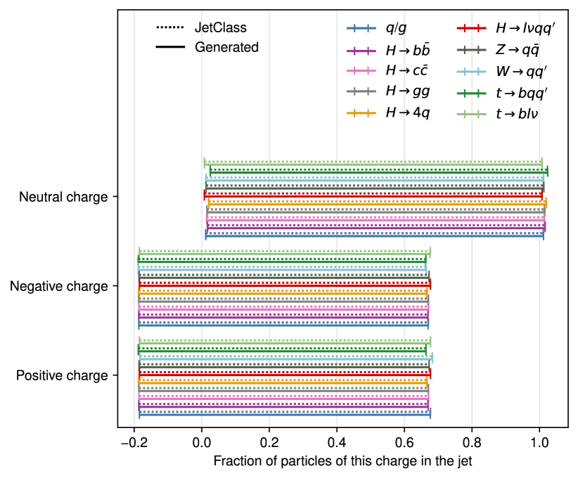
Figure 7: Average fraction of jet constituents of different electric charge. For each jet type, the intervals show the mean value over all evaluated jets with up and down variations of one standard deviation. The dotted lines show the values obtained for real jets from the JetClass dataset and the solid lines show the values obtained for the generated jets.

Appendix B Hyperparameters

The hyperparameters used for our generative model are listed in Table 5. This choice of hyperparameters was found to lead to the best performance among several different configurations, though they were not extensively optimized.

Table 5: Hyperparameters used for the baseline EPiC-FM model.

Hyperparameter	Value
Number of EPiC layers	20
Global dim. in EPiC layers	16
Hidden dim. in EPiC layers	300
ODE solver	midpoint
Number of function evaluations	200
Activation function	LeakyReLU(0.01)
AdamW [50] learning rate	0.001
Weight decay	0.00005
Learning rate scheduler	CosineAnnealing
Linear warm-up	20 epochs
Total number of epochs	EPiC-FM: 500
	EPiC-FM-kin: 500
	EPiC-FM-top: 1000
	EPiC-FM-kintop: 1000
Batch size	1024
Trainable parameters	8,504,698
Training jets	3M (300k per jet type)

The hyperparameters used for the classifier test are shown in Table 6. The model weights are initialized using the pre-trained ParT-kin model from https://github.com/jet-universe/particle_transformer.

Table 6: Hyperparameters used for the classifier test with the ParT-kin [45] model.

Hyperparameter	Value
AdamW [50] learning rate	0.001
Weight decay	0.00005
Learning rate scheduler	Constant
Total number of epochs	100
Batch size	256
Trainable parameters	$2\,141\,134$
Training jets	$500\,000$
Validation jets	$100\,000$
Testing jets	$400\,000$

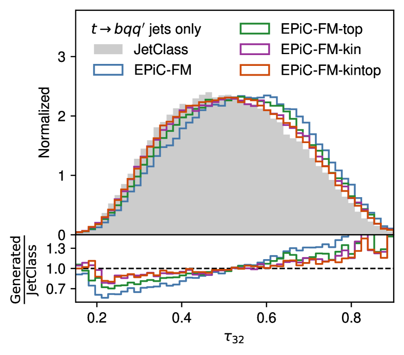
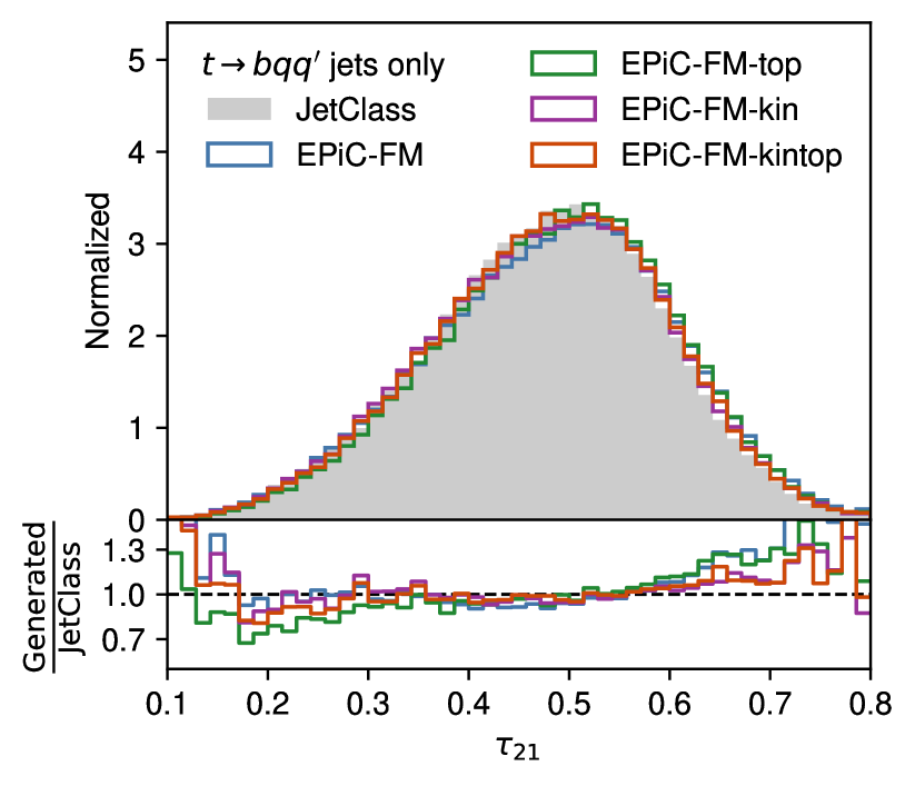
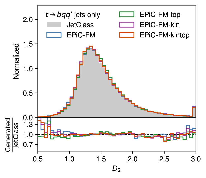
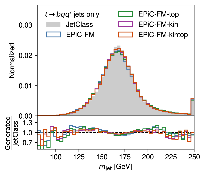
Figure 8: Comparison of the jet substructure of $t\to bqq^{\prime}$ jets for the four different models. The models EPiC-FM-top and EPiC-FM-kintop were trained on $t\to bqq^{\prime}$ jets only.

Table 7: KL divergence metrics for the four different models used for improving the modeling of $t\to bqq^{\prime}$ jets. The models EPiC-FM-top and EPiC-FM-kintop were trained on $t\to bqq^{\prime}$ jets only.

	$\mathrm{KL}^{m_{\mathrm{jet}}}~{}(\times 10^{-3})$	$\mathrm{KL}^{\tau_{21}}~{}(\times 10^{-3})$	$\mathrm{KL}^{\tau_{32}}~{}(\times 10^{-3})$	$\mathrm{KL}^{D_{2}}~{}(\times 10^{-3})$
Truth ($t\to bqq^{\prime}$)	$1.860\,03\pm 0.248\,93$	$1.998\,56\pm 0.261\,65$	$2.059\,73\pm 0.235\,60$	$1.936\,81\pm 0.308\,60$
EPiC-FM ($t\to bqq^{\prime}$)	$4.668\,58\pm 0.610\,07$	$7.873\,70\pm 0.859\,60$	$29.864\,26\pm 1.039\,10$	$2.952\,29\pm 0.431\,81$
EPiC-FM-kin ($t\to bqq^{\prime}$)	$2.660\,65\pm 0.259\,41$	$3.158\,77\pm 0.382\,34$	$6.236\,49\pm 0.779\,57$	$2.100\,68\pm 0.327\,21$
EPiC-FM-top ($t\to bqq^{\prime}$)	$4.330\,50\pm 0.429\,34$	$7.784\,51\pm 0.635\,32$	$13.270\,51\pm 0.853\,76$	$3.144\,86\pm 0.250\,37$
EPiC-FM-kintop ($t\to bqq^{\prime}$)	$2.562\,37\pm 0.382\,24$	$3.496\,19\pm 0.316\,03$	$4.839\,99\pm 0.632\,90$	$2.317\,88\pm 0.342\,19$

Appendix C Further studies for hadronic top jet modeling

Since $t\to bqq^{\prime}$ jets were found to be the most challenging jet type to model, further studies are performed to improve and investigate the modeling of those jets. To this end, we compare our baseline model, which we refer to in the following as EPiC-FM, to three additional models:

• EPiC-FM-top is trained on the same features as the baseline model, but only the $t\to bqq^{\prime}$ jets from the training dataset are used for training;

• EPiC-FM-kin is trained on kinematic features only (i.e. $p_{\mathrm{T}}^{\text{rel}}$, $\eta^{\text{rel}}$ and $\phi^{\text{rel}}$) but uses the full training dataset and

• EPiC-FM-kintop is trained on kinematic features only (i.e. $p_{\mathrm{T}}^{\text{rel}}$, $\eta^{\text{rel}}$ and $\phi^{\text{rel}}$) and only uses the $t\to bqq^{\prime}$ jets from the training dataset.

The KL divergence values for the jet-level observables are listed for all models in Table 7 and the substructure of the generated $t\to bqq^{\prime}$ jets for the three different models is shown in Figure 8. It can be seen that the models that are restricted to kinematic features show better agreement with the real jets than the two models that are trained on all features. This is also confirmed by the KL divergence, which show that the EPiC-FM-kin model has a significantly smaller KL divergence than the EPiC-FM model for all substructure observables. These observations lead to the conclusion that the additional features slightly confuse the modeling of the kinematic features which results in a worse representation of the substructure. However, the jets are still modeled well in the case of all features, and the ability to model the discrete features extends the usability of such generative models.

The model that is restricted to $t\to bqq^{\prime}$ jets and kinematic features, EPiC-FM-kintop, shows similar improvements as the EPiC-FM-kin model. However, while there is a slight improvement over the EPiC-FM-kin model in the KL divergence for $\tau_{32}$, the KL divergence for $\tau_{21}$ and $D_{2}$ is slightly larger than for the kin-only model. In the case where all features are used, i.e. when comparing the EPiC-FM-top model to the baseline model EPiC-FM, we see an improvement in $\tau_{32}$, while not seeing an improvement in the KL divergence of $\tau_{21}$ and $D_{2}$. Thus, the single jet-type model performs better than the model that is trained on all jet types if all features are used, while there is no clear improvement by training solely on $t\to bqq^{\prime}$ jets if only kinematic features are used.

References

- Sjöstrand et al. [2015] T. Sjöstrand, S. Ask, J. R. Christiansen, R. Corke, N. Desai, P. Ilten, S. Mrenna, S. Prestel, C. O. Rasmussen, and P. Z. Skands, Computer Physics Communications 191, 159–177 (2015).
- Bähr et al. [2008] M. Bähr, S. Gieseke, M. A. Gigg, D. Grellscheid, K. Hamilton, O. Latunde-Dada, S. Plätzer, P. Richardson, M. H. Seymour, A. Sherstnev, and B. R. Webber, The European Physical Journal C 58, 639–707 (2008).
- Evans and Bryant [2008] L. Evans and P. Bryant, JINST 3, S08001 (2008).
- Buhmann et al. [2023a] E. Buhmann, C. Ewen, G. Kasieczka, V. Mikuni, B. Nachman, and D. Shih, “Full Phase Space Resonant Anomaly Detection,” (2023a), arXiv:2310.06897 [hep-ph] .
- Kansal et al. [2022a] R. Kansal, J. Duarte, H. Su, B. Orzari, T. Tomei, M. Pierini, M. Touranakou, J.-R. Vlimant, and D. Gunopulos, “Particle Cloud Generation with Message Passing Generative Adversarial Networks,” (2022a), arXiv:2106.11535 [cs.LG] .
- Käch et al. [2022] B. Käch, D. Krücker, I. Melzer-Pellmann, M. Scham, S. Schnake, and A. Verney-Provatas, “JetFlow: Generating Jets with Conditioned and Mass Constrained Normalising Flows,” (2022), arXiv:2211.13630 [hep-ex] .
- Buhmann et al. [2023b] E. Buhmann, G. Kasieczka, and J. Thaler, “EPiC-GAN: Equivariant Point Cloud Generation for Particle Jets,” (2023b), arXiv:2301.08128 [hep-ph] .
- Leigh et al. [2023a] M. Leigh, D. Sengupta, G. Quétant, J. A. Raine, K. Zoch, and T. Golling, “PC-JeDi: Diffusion for Particle Cloud Generation in High Energy Physics,” (2023a), arXiv:2303.05376 [hep-ph] .
- Mikuni et al. [2023] V. Mikuni, B. Nachman, and M. Pettee, “Fast Point Cloud Generation with Diffusion Models in High Energy Physics,” (2023), arXiv:2304.01266 [hep-ph] .
- Käch and Melzer-Pellmann [2023] B. Käch and I. Melzer-Pellmann, “Attention to Mean-Fields for Particle Cloud Generation,” (2023), arXiv:2305.15254 [hep-ex] .
- Buhmann et al. [2023c] E. Buhmann, S. Diefenbacher, E. Eren, F. Gaede, G. Kasieczka, A. Korol, W. Korcari, K. Krüger, and P. McKeown, “CaloClouds: Fast Geometry-Independent Highly-Granular Calorimeter Simulation,” (2023c), arXiv:2305.04847 [physics.ins-det] .
- Leigh et al. [2023b] M. Leigh, D. Sengupta, J. A. Raine, G. Quétant, and T. Golling, “PC-Droid: Faster diffusion and improved quality for particle cloud generation,” (2023b), arXiv:2307.06836 [hep-ex] .
- Buhmann et al. [2023d] E. Buhmann, F. Gaede, G. Kasieczka, A. Korol, W. Korcari, K. Krüger, and P. McKeown, “CaloClouds II: Ultra-Fast Geometry-Independent Highly-Granular Calorimeter Simulation,” (2023d), arXiv:2309.05704 [physics.ins-det] .
- Buhmann et al. [2023e] E. Buhmann, C. Ewen, D. A. Faroughy, T. Golling, G. Kasieczka, M. Leigh, G. Quétant, J. A. Raine, D. Sengupta, and D. Shih, “EPiC-ly Fast Particle Cloud Generation with Flow-Matching and Diffusion,” (2023e), arXiv:2310.00049 [hep-ph] .
- Vaswani et al. [2017] A. Vaswani et al., in Proceedings of Advances in Neural Information Processing Systems, Vol. 30 (2017) pp. 5999–6009, 1706.03762 .
- Sohl-Dickstein et al. [2015] J. Sohl-Dickstein, E. A. Weiss, N. Maheswaranathan, and S. Ganguli, “Deep Unsupervised Learning using Nonequilibrium Thermodynamics,” (2015), arXiv:1503.03585 [cs.LG] .
- Song and Ermon [2020a] Y. Song and S. Ermon, “Generative Modeling by Estimating Gradients of the Data Distribution,” (2020a), arXiv:1907.05600 [cs.LG] .
- Song and Ermon [2020b] Y. Song and S. Ermon, “Improved Techniques for Training Score-Based Generative Models,” (2020b), arXiv:2006.09011 [cs.LG] .
- Ho et al. [2020] J. Ho, A. Jain, and P. Abbeel, “Denoising Diffusion Probabilistic Models,” (2020), arXiv:2006.11239 [cs.LG] .
- Song et al. [2021] Y. Song, J. Sohl-Dickstein, D. P. Kingma, A. Kumar, S. Ermon, and B. Poole, “Score-Based Generative Modeling through Stochastic Differential Equations,” (2021), arXiv:2011.13456 [cs.LG] .
- Liu et al. [2022] X. Liu, C. Gong, and Q. Liu, “Flow Straight and Fast: Learning to Generate and Transfer Data with Rectified Flow,” (2022), arXiv:2209.03003 [cs.LG] .
- Albergo and Vanden-Eijnden [2023] M. S. Albergo and E. Vanden-Eijnden, “Building Normalizing Flows with Stochastic Interpolants,” (2023), arXiv:2209.15571 [cs.LG] .
- Lipman et al. [2023] Y. Lipman, R. T. Q. Chen, H. Ben-Hamu, M. Nickel, and M. Le, “Flow Matching for Generative Modeling,” (2023), arXiv:2210.02747 [cs.LG] .
- Tong et al. [2023] A. Tong, N. Malkin, G. Huguet, Y. Zhang, J. Rector-Brooks, K. Fatras, G. Wolf, and Y. Bengio, “Improving and generalizing flow-based generative models with minibatch optimal transport,” (2023), arXiv:2302.00482 [cs.LG] .
- Agostinelli et al. [2003] S. Agostinelli et al., Nuclear Instruments and Methods in Physics Research Section A: Accelerators, Spectrometers, Detectors and Associated Equipment 506, 250 (2003).
- Allison et al. [2006] J. Allison et al., IEEE Trans. Nucl. Sci. 53, 270 (2006).
- Allison et al. [2016] J. Allison et al., Nuclear Instruments and Methods in Physics Research Section A: Accelerators, Spectrometers, Detectors and Associated Equipment 835, 186 (2016).
- Acosta et al. [2023] F. T. Acosta, V. Mikuni, B. Nachman, M. Arratia, B. Karki, R. Milton, P. Karande, and A. Angerami, “Comparison of point cloud and image-based models for calorimeter fast simulation,” (2023), arXiv:2307.04780 [cs.LG] .
- Scham et al. [2023] M. A. W. Scham, D. Krücker, B. Käch, and K. Borras, “DeepTreeGAN: Fast Generation of High Dimensional Point Clouds,” (2023), arXiv:2311.12616 [hep-ex] .
- Otten et al. [2021] S. Otten, S. Caron, W. de Swart, M. van Beekveld, L. Hendriks, C. van Leeuwen, D. Podareanu, R. Ruiz de Austri, and R. Verheyen, Nature Commun. 12, 2985 (2021), arXiv:1901.00875 [hep-ph] .
- Hashemi et al. [2019] B. Hashemi, N. Amin, K. Datta, D. Olivito, and M. Pierini, “LHC analysis-specific datasets with Generative Adversarial Networks,” (2019), arXiv:1901.05282 [hep-ex] .
- Di Sipio et al. [2019] R. Di Sipio, M. Faucci Giannelli, S. Ketabchi Haghighat, and S. Palazzo, JHEP 08, 110 (2019), arXiv:1903.02433 [hep-ex] .
- Butter et al. [2019] A. Butter, T. Plehn, and R. Winterhalder, SciPost Phys. 7, 075 (2019), arXiv:1907.03764 [hep-ph] .
- Alanazi et al. [2021] Y. Alanazi, N. Sato, T. Liu, W. Melnitchouk, P. Ambrozewicz, F. Hauenstein, M. P. Kuchera, E. Pritchard, M. Robertson, R. Strauss, L. Velasco, and Y. Li, in Proceedings of the Thirtieth International Joint Conference on Artificial Intelligence, IJCAI-21, edited by Z.-H. Zhou (IJCAI, 2021) p. 2126, 2001.11103 .
- Butter et al. [2021] A. Butter, T. Heimel, S. Hummerich, T. Krebs, T. Plehn, A. Rousselot, and S. Vent, “Generative Networks for Precision Enthusiasts,” (2021), arXiv:2110.13632 [hep-ph] .
- Butter et al. [2023a] A. Butter, N. Huetsch, S. P. Schweitzer, T. Plehn, P. Sorrenson, and J. Spinner, “Jet Diffusion versus JetGPT – Modern Networks for the LHC,” (2023a), arXiv:2305.10475 [hep-ph] .
- Butter et al. [2023b] A. Butter, T. Jezo, M. Klasen, M. Kuschick, S. P. Schweitzer, and T. Plehn, “Kicking it Off(-shell) with Direct Diffusion,” (2023b), arXiv:2311.17175 [hep-ph] .
- Kansal et al. [2022b] R. Kansal, J. Duarte, H. Su, B. Orzari, T. Tomei, M. Pierini, M. Touranakou, J.-R. Vlimant, and D. Gunopulos, “JetNet,” (2022b).
- Kansal et al. [2022c] R. Kansal, J. Duarte, H. Su, B. Orzari, T. Tomei, M. Pierini, M. Touranakou, J.-R. Vlimant, and D. Gunopulos, “JetNet150,” (2022c).
- Coleman et al. [2018] E. Coleman, M. Freytsis, A. Hinzmann, M. Narain, J. Thaler, N. Tran, and C. Vernieri, JINST 13, T01003 (2018).
- Krause and Shih [2023] C. Krause and D. Shih, Physical Review D 107 (2023), 10.1103/physrevd.107.113003.
- Das et al. [2023] R. Das, L. Favaro, T. Heimel, C. Krause, T. Plehn, and D. Shih, “How to Understand Limitations of Generative Networks,” (2023), arXiv:2305.16774 [hep-ph] .
- Qu et al. [2022a] H. Qu, C. Li, and S. Qian, “JetClass: A Large-Scale Dataset for Deep Learning in Jet Physics,” (2022a).
- Chen et al. [2019] R. T. Q. Chen, Y. Rubanova, J. Bettencourt, and D. Duvenaud, “Neural Ordinary Differential Equations,” (2019), arXiv:1806.07366 [cs.LG] .
- Qu et al. [2022b] H. Qu, C. Li, and S. Qian, in Proceedings of the 39th International Conference on Machine Learning (2022) pp. 18281–18292, arXiv:2202.03772 [hep-ph] .
- Alwall et al. [2014] J. Alwall, R. Frederix, S. Frixione, V. Hirschi, F. Maltoni, O. Mattelaer, H.-S. Shao, T. Stelzer, P. Torrielli, and M. Zaro, Journal of High Energy Physics 2014 (2014), 10.1007/jhep07(2014)079.
- de Favereau et al. [2014] J. de Favereau, C. Delaere, P. Demin, A. Giammanco, V. Lemaître, A. Mertens, and M. Selvaggi, Journal of High Energy Physics 2014 (2014), 10.1007/jhep02(2014)057.
- The CMS Collaboration [2008] The CMS Collaboration, JINST 3, S08004 (2008).
- Cacciari et al. [2008] M. Cacciari, G. P. Salam, and G. Soyez, Journal of High Energy Physics 2008, 063–063 (2008).
- Loshchilov and Hutter [2019] I. Loshchilov and F. Hutter, “Decoupled Weight Decay Regularization,” (2019), arXiv:1711.05101 [cs.LG] .
- Paszke et al. [2019] A. Paszke et al., in Advances in Neural Information Processing Systems 32, edited by H. Wallach, H. Larochelle, A. Beygelzimer, F. d'Alché-Buc, E. Fox, and R. Garnett (Curran Associates, Inc., 2019) pp. 8024–8035.
- Falcon and The PyTorch Lightning team [2019] W. Falcon and The PyTorch Lightning team, “PyTorch Lightning,” (2019).
- Thaler and Tilburg [2011] J. Thaler and K. V. Tilburg, JHEP 03, 015 (2011).
- Larkoski et al. [2016] A. J. Larkoski, I. Moult, and D. Neill, “Analytic Boosted Boson Discrimination,” (2016), arXiv:1507.03018 [hep-ph] .
- Larkoski et al. [2013] A. J. Larkoski, G. P. Salam, and J. Thaler, JHEP 06, 108 (2013).
- Alimena et al. [2020] J. Alimena et al., Journal of Physics G: Nuclear and Particle Physics 47, 090501 (2020).