Revolutionizing Forensic Toolmark Analysis:
An Objective and Transparent Comparison Algorithm

Abstract

Forensic toolmark comparisons are currently performed subjectively by humans, which leads to a lack of consistency and accuracy. There is little evidence that examiners can determine whether pairs of marks were made by the same tool or different tools. There is also little evidence that they can make this classification when marks are made under different conditions, such as different angles of attack or direction of mark generation. We generate original toolmark data in 3D, extract the signal from each toolmarks, and train an algorithm to compare toolmark signals objectively. We find that toolmark signals cluster by tool, and not by angle or direction. That is, the variability within tool, regardless of angle/direction, is smaller than the variability between tools. The known-match and known-non-match densities of the similarities of pairs of marks have a small overlap, even when accounting for dependencies in the data, making them a useful instrument for determining whether a new pair of marks was made by the same tool. We provide a likelihood ratio approach as a formal method for comparing toolmark signals with a measure of uncertainty. This empirically trained, open-source method can be used by forensic examiners to compare toolmarks objectively and thus improve the reliability of toolmark comparisons. This can, in turn, reduce miscarriages of justice in the criminal justice system.

1 Significance Statement

Forensic toolmark comparisons are a crucial part of the criminal justice system but currently rely on subjective judgments. This can lead to lower accuracy, inconsistency in examiners’ judgments, and a lack of transparency in the examiners’ decision process. Toolmarks can be made at different angles and directions. This complexity has made it difficult to develop objective methods for toolmark comparison. This article summarizes a three-year research study designed to develop an objective method of toolmark comparisons. Using experimental data that we created in a controlled setting, we assess whether toolmarks can be compared reliably, despite being made under different conditions. This article aims to improve the consistency and validity of the discipline of forensic toolmark comparisons, thus strengthening forensic science.

2 Introduction

A 2009 report from the National Academies of Science entitled “Strengthening Forensic Science in the United States: A Path Forward” found significant problems with forensic science practice. In 2016, a report from the President’s Council of Advisors on Science and Technology (PCAST) provided an updated review of forensic disciplines, and found many of the same problems as in the 2009 NRC report. Both reports recommended developing objective methods for forensic comparisons so the results do not depend on the investigator. The reliance on subjective, human judgment can lead to unnecessary errors. Because how and why examiners make decisions is unknown, subjectivity in forensic analysis can lead to lower accuracy, a lack of consistency in examiners’ judgments, and a lack of transparency [Kafadar, 2019]. In response to these government reports, we propose an algorithm to make toolmark comparisons objective. This method is produces results with uncertainty measures, it is consistent in its performance, and it is transparent. This contribution promises to improve the reliability of forensic toolmark comparisons.

3 Background

Tools like screwdrivers, crowbars, and wire cutters are often used during the commission of a crime, such as breaking into a property or making an explosive device [Baiker-Sørensen et al., 2020]. The goal of forensic toolmark examiners is to determine whether a candidate tool, if available, made the mark found at the crime scene. An examiner might also compare marks on separate pieces of evidence of unknown source to determine whether they come from the same source [Baldwin et al., 2013]. In the laboratory, the examiner generates test marks with the candidate tool at different angles and directions, and then compares the crime scene mark and test marks [Petraco, 2010]. Conclusions from these comparisons can and are used as evidence in legal cases [Nichols, 1997, Nichols, 2003].

The decision about whether two toolmarks were made by the same tool relies on subjective, human judgment. Toolmark examiners compare the marks subjectively by using a comparison light microscope, which depicts the striation marks as light and dark patterns in 2D [Petraco, 2010]. Then, the examiner must decide whether the marks were made by the same source or different source by determining whether the “surface contours of two toolmarks are in ‘sufficient agreement”’ based on the examiner’s opinion that another tool could not have made the marks [AFTE, 1998]. How the examiner decides what “sufficient agreement” is is purely subjective.

Much of the attention in objective methods has focused on firearms, not handheld tools. This is because the two categories are usually combined and evaluated together, but the research on handheld tools is more challenging because of the “degrees of freedom” problem. Whereas in firearms the shape of a toolmark depends largely on factors that the user cannot control, in non-firearm toolmarks, factors (degrees) such as the angle of attack and the direction in which the mark was made affect the shape of the toolmark [Petraco, 2010, Baldwin et al., 2013]. Researchers have developed some objective methods to compare non-firearm toolmarks [Baiker et al., 2015, Lock and Morris, 2013, Macziewski et al., 2017, Spotts et al., 2015, M.S. et al., 2015], and have tried to address the “degrees of freedom” problem in limited ways. For instance, [Baiker et al., 2015] find that at angles of attack of more than 30 degrees, the marks made by the same tool can look quite different from each other. Since there are so many ways to make a mark, it is difficult to study comparisons systematically. For this reason, anecdotally, examiners have said that toolmark comparison is “more of an art than a science.” We propose studying this problem systematically, and investigate and objective approach.

Specifically, this article presents three contributions to the field. First, we generate original data. Datasets of toolmarks are available in forensic laboratories, but they are often unlabeled, do not have multiple replicates, and do not have marks made by the same tool under different controlled conditions. Furthermore, analysis in laboratories is usually available in 2D, and 3D data has been shown to provide much better results since it contains precise information about the depth of the marks [Vorburger et al., 2007, Baiker et al., 2014]. We genearte toolmarks from consecutively manufactured, previously unused, flat-head screwdrivers. We make eight replicates per source and we make marks under different conditions (shifting angle of attack and direction of mark generation). Second, we use the GelSight portable handheld 3D scanner, which measures the 3D topography of a solid surface using elastomeric tactile sensor technology, to generate high-resolution digital 3D images of the toolmarks. Third, we produce an open-source algorithm, trained with our empirical data, for the comparison of signatures extracted from the 3D scans. The algorithm classifies whether a pair of toolmarks was made by the same tool or by different tools, and it produces likelihood ratio estimates to determine, for a new pair of toolmarks, the weight of the evidence under the same-source and different-source hypotheses.

Section 4.1 describes the data generation process, Section 4.2 describes the methods, including clustering, density fitting, and likelihood ratio test. To clarify some terminology, we use the term tool to mean a single screwdriver, source to mean the side of a screwdriver tip (since sides A and B of each screwdriver are different from each other), mark to mean the striation marks made by a screwdriver on lead, scan to mean the 2D topographics image obtained for each mark in 3D, signal to mean the 2D signal we extracted computationally from a mark, replicate to mean one of the repeated marks made by a single tool at the same condition (e.g., angle and direction), and condition to refer to a specific combination of angle and direction under which a mark is made.

4 Materials and Methods

4.1 Materials

The materials for the experiments are 20 small slotted consecutively manufactured screwdrivers and 3 large slotted consecutively manufactured screwdrivers. We choose consecutively manufactured tools because they provide the most difficult scenario, as tools manufactured closer to each other in time are more similar to each other than tools manufactured at different times [Nichols, 1997, Nichols, 2003]. An automated Siepmann grinding wheel is used to form the final tip geometry in the manufacturing process. Since the grinding wheel is used independently for each side of the screwdriver, the marks on the two sides are likely very different from each other. Klein tools, the manufacturer, sells tools to a variety of suppliers, including Home Depot, where they may be purchased for amounts between $10 and $15. Thus, the tools are available to the general public, so they could be used in the commission of a crime, such as the building of an explosive device. We select flat-head screwdrivers for our study because they can be used to generate striation marks on a flat surface, unlike other tools such as wire cutters that have multiple surfaces that interact with each other.

To generate toolmarks in a controlled and replicable way, we use a mechanical rig, which we obtained from the authors of [Zheng et al., 2014] and modified in the Manufacturing & Fabrication Services shop the University of Pennsylvania Department of Mechanical Engineering & Applied Mechanics. The rig has a motorized slide that controls the direction and speed of the plate to allow for the generation of replicable marks. We generate the toolmarks on lead plates because we find that lead preserves fine details in the striations [Baiker et al., 2015], and it allows us to create smooth marks without high forces, which can make the slide motor stop and create jitter effects.

To scan the toolmarks in 3D, we use a handheld scanner sold by GelSight. The GelSight instrument’s resolution [GelSight, 2023] in the $x-y$ (horizontal) plane is 3.45 microns, and the accuracy in the $z$ (vertical) direction is 4 microns. This scanner is hand-held and powered by a tablet, which would make it easy to use at crime scenes. It cannot be used to scan very deep marks (it has been tested up to 90 microns in depth [GelSight, 2023]) or sharp-angled surfaces that could break the gel’s surface. However, it is very well-suited for scanning striation marks like the ones in this experiment and likely for many marks found at crime scenes.

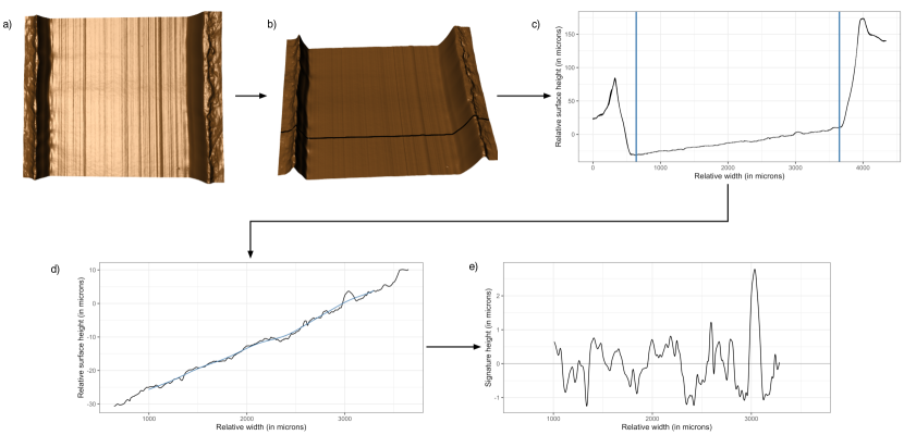
Figure 1: Processing of the 3D images to extract the signal. a) shows a rendering of a toolmark scan. In b) the black vertical line highlights the location of the crosscut. c) Shows the height profile corresponding to the crosscut. The blue vertical lines mark the range of the scan marks. Outside this range, the scan shows structure related to the plate. d) shows a zoom into the mark-related range. In blue, a line showing Gaussian smoothing is shown. In e) the final signal of the plate is shown; for illustration, another signal is overlaid. The second signal is of a replicate mark created with the same screwdriver and side.

To extract the digital signals from the 3D scans (see Figure 1), we select a cut across the scan and extracted a 2d profile from the scan using the R package bulletxtrctr [Hofmann et al., 2022]. To prepare the data for analysis, we crop the edges of the profile and apply Gaussian smoothing to the data to model macro structures, such as the plate’s shape and any scanning-specific trends. We define the signal of the screwdriver side as the difference between the profile’s height values and the fitted structure. Figure 1e shows the signals extracted from two different replicate marks, made by the same source. The similarities between the two signals are obvious, but there are also clear differences between them, due to differences in the actual marks and scanning.

Finally, we align the signals. For Figures 2-4, the signals are aligned with respect to ‘the first’ signal in the set. For the clustering and the density analysis we use similarity measures that are extracted from pairwise aligned signals. We use a sliding window approach in which signals are compared in pairs by sliding one over the other, to find the lag that produces the maximum correlation between the signals.

We use a factorial design for the toolmarks generation, to allow for the study of the variability within source and between sources of marks, and how this changes as the conditions of of angle of attack and direction of mark generation change. The factors are the angle and direction. The rest of the marks are made with small screwdrivers. We generate three sets of marks, which we call experiments, for a total of 560 marks. Table 1 shows the combination of conditions for each. As can be seen in Table 1 below, we generate eight replicates per tool-side under the same conditions.

Table 1: Experimental design. For each of the three experiments (1, 2, and 3), we altered a different variable (tool, angle, direction) and generated replicates at each condition.

experiment	Num. of tools (Size)	Sides	Angles	Directions	Replicate	Num. of marks
1: Tool	20 (S)	A, B	80	Pull	8	320
2: Angle	3 (L)	A, B	60, 70, 80	Pull	8	144
3: Direction	3 (S)	A, B	80	Pull, push	8	96

Experiments 1, 2, and 3 allow us to study the variability between marks made by the same tool, since there are 8 replicates made under each condition. For example, Figure 2 shows the marks made by a screwdriver’s two sides, with eight replicates per side. Visually, the replicates look very similar to each other, while marks from the two sides A and B look very different from each other. experiment 1 includes marks produced at a constant angle and direction; experiments 2 and 3 focus on the variability between marks made at different angles and directions. Figures 3 and 4 show that the marks vary some when made at different angles and directions. We quantify these differences in the Methods and Results sections.

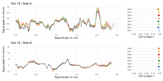
Figure 2: Tool 1 signals, aligned by the set of replicates from one source, where the black signal is the average of the rest.

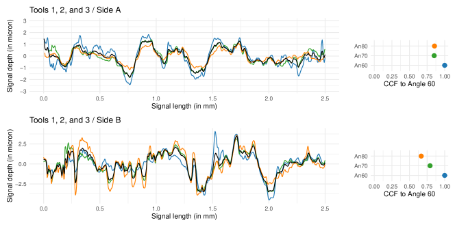
Figure 3: Large tool 1 signals, averaged by replicates, and aligned by angle of attack (60, 70, 80), where the black signal is the average of the rest.

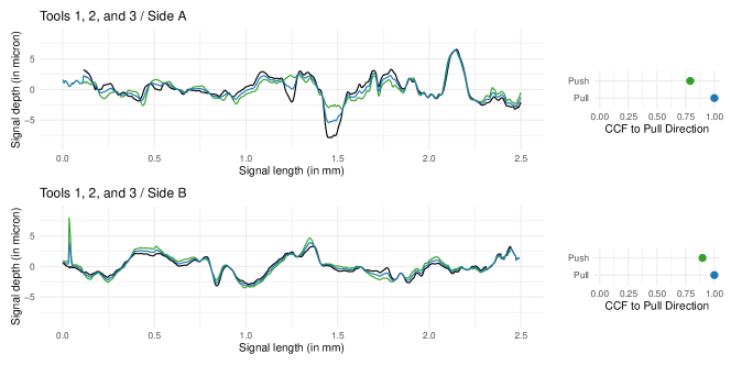
Figure 4: Small large tool 1 signals, averaged by replicates, and aligned by direction (pull and push), where the black signal is the average of the rest.

4.2 Methods

Our goal is to develop a method to classify, for a new pair of toolmarks, whether it was made by the same tool or not. To do this, we first cluster the signals to study the variability within tool and the variability between tools, both at a fixed setting and when varying angle and direction. This is an exploratory step that allows us to know which pairs we should consider same-source or different-source in a data-driven way. Second, we plot a density of similarity scores observed among known matches and a density of scores observed among known non-matches. We seek to find 1) whether the densities are separated such that there is a smal overlap between them, and if so 2) where, in terms of similarity, the two densities cross, i.e., the threshold. We use the threshold to classify between whether there is more support for the evidence given the prosecution or the defense hypothesis. This threshold helps later test the performance of the classifier. We then fit distributions on the similarity densities to allow for the estimation of likelihood ratios for new pairs of toolmarks.

Clustering allows us to see whether varying angle and direction leads to great differences in the signals, an effect that could lead toolmark comparisons to be very challenging since for each tool examiners might have to consider a great (possibly infinite) number of marks.

We cannot simply assume that marks made at different angles and directions, by the same tool-side, can be considered same- or different-source, since it is possible that at different settings, marks look extremely different from each other. Previous research suggests that different sides of a screwdriver produce signals that should be considered as different sources. Moreover signals made at angles of attack greater than 15 degrees difference could not be considered same-source because they were too different from each other [Hadler and Morris, 2018].

This clustering test is a data-driven method to determine whether we should consider pairs of marks to be same-source or different-source. It also helps compare the within-tool variability across replicates to the between-tool variability, for each tool. Of course, this is limited to the training data that we produced. Thus, clustering is a preliminary test for us to select which pairs to include in the densities in the rest of our methodology.

For clustering, the first step is to calculate the similarity matrix for each experiment, meaning all the pairwise cross-correlation functions in the data. For each experiment, given the similarity matrix $S$, the next step is to cluster the toolmarks into different groups based on $S$. In general the goal of clustering algorithms is to partition data into different groups such that data within a group are more similar than data from different groups. For Euclidean data, $k$-means is a popular clustering method in which the mean of the data within one group meaningfully represent the “center” of the cluster. However, this property does not hold for non-Euclidean data where the similarity measure is arbitrary [Schubert and Rousseeuw, 2019]. Due to the nature of the toolmarks similarity, we use the partition around medoids (PAM) algorithm [Dodge, 1987, Kaufman and Rousseeuw, 2009] which is a generalization of $k$-means to the non-Euclidean data. The goal of the algorithm is to minimize the average dissimilarity of objects to their closest selected object. The medoid of a set $C$ is defined as the object with the smallest sum of dissimilarities (or, equivalently, smallest average) to all other objects in the set hence it can be viewed as a representative of the objects in this cluster. In summary, the PAM algorithm searches for $k$ representative objects in the given dataset (denoted as $k$ medoids) and assigns each point to the closest medoid to create clusters. The objective is to minimize the sum of dissimilarities between the objects within a cluster and the center of the same cluster (i.e, medoid).

Before calculating the clustering result for each experiment, we need to select the number of clusters $k$ for each experimental setting, that is, to identify the optimal number of clusters to include. To this end, we need a measure for how “good” a clustering algorithm is. The Silhouette score [Rousseeuw, 1987] evaluates clustering performance based on the pairwise difference between within-cluster and between-cluster distances. Given a similarity matrix $S$ and a cluster $C_{i}$, for each data $n\in C_{i}$, we first calculate,

$$\begin{split}a(n)&=\frac{1}{|C_{i}|-1}\sum_{m\in C_{i},m\neq n}S_{mn}\\ b(n)&=\min_{j\neq i}\frac{1}{|C_{j}|}\sum_{m\in C_{j}}S_{mn},\end{split}$$ (1)

as the mean within-cluster distance and smallest between-cluster distance. Here, we denote $|C_{i}|$ as the size of the $i$-th cluster for $i=1,2,\dots,k$. The Silhouette score for data $n\in C_{i}$ is then defined as

$$s(n)=\frac{b(n)-a(n)}{\max\{a(n),b(n)\}}$$ (2)

if $|C_{i}|>1$ and $s(n)=0$ otherwise. By definition, $-1\leq s(n)\leq 1$, and we define the Silhouette score for the clustering method as the average Silhouette score across all samples.

We then vary the number of clusters and apply PAM clustering for each possible $k$. For the clustering result at each given cluster number, we calculate the average Silhouette scores across all samples. We then choose the cluster number that maximizes the Silhouette score. Intuitively, this corresponds to the cluster number that yields the “best partition” of the data.

We introduce a score-based likelihood-ratio approach to make forensic toolmark comparisons. In a criminal case, forensic examiners analyze the evidence and present their findings to the trier of fact, who combines all the information presented in the case to deliver a final decision about the defendant’s guilt. Under a probabilistic framework, the trier of fact compares two propositions referred to as the prosecution hypothesis ($H_{p}$) and the defense hypothesis ($H_{d}$) conditional on the evidence observed [Aitken and Taroni, 2004]. Applying the ratio form of Bayes’ theorem, the trier of fact’s task is to estimate,

$$\underbrace{\frac{P(H_{p}|E)}{P(H_{d}|E)}}_{\text{Posterior odds}}=\underbrace{{\frac{P(E|H_{p})}{P(E|H_{d})}}}_{\text{Likelihood ratio}}\underbrace{\frac{P(H_{p})}{P(H_{d})}}_{\text{Prior odds}}.$$ (3)

In other words, the trier or fact’s prior beliefs regarding the hypotheses are updated via a likelihood ratio. Forensic experts are advised to present their findings as a likelihood ratio by scientific and professional organizations [Willis et al., 2015].

In the case of forensic toolmarks, experts may be presented with a pair of questioned marks as evidence $E=(E_{x},E_{y})$ and asked to evaluate if a common tool produced the two marks. Under the common-source framework [Ommen and Saunders, 2018], we can state the propositions as $H_{p}:$ Marks $E_{x}$ and $E_{y}$ were made by the same unknown tool, and $H_{d}:$ Marks $E_{x}$ and $E_{y}$ were made by different unknown tools.

To assess these competing propositions, forensic experts can rely on observed features of the questioned mark. Let $u_{i}$ denote the features of $E_{i}(i=x,y)$. If the joint distribution of the features under each of the competing propositions, denoted by $f(u_{x},u_{y}|H_{j})(j=d,p)$, is known, the likelihood ratio could be computed,

$$LR=\frac{f(u_{x},u_{y}|H_{p})}{f(u_{x},u_{y}|H_{d})}.$$ (4)

A $LR>1$ indicates that the priors are being updated towards the prosecutor, meaning the evidence supports the prosecutor’s proposition, while a $LR<1$ indicates that the priors are being updated towards the defense.

To estimate the joint probability model, researchers use a sample of the background population or reference set composed of information previously collected. Let $A$ denote the reference set, $E^{A}_{ij}$ an individual item $j(j=1,\dots,n_{i})$ from source $i$, $(i=1,\dots,m)$ and $A_{ij}$ the corresponding measurement from item $j$ from source $i$.

[Ommen and Saunders, 2018] express the proposition and the process that generated the data available to the expert as a sampling model. They consider that the reference set $A$ was generated first by randomly sampling $m$ sources from a reference population and, within each source, sampling $n_{i}$ items. To do this, experts have relied on machine learning comparison metrics and density estimation procedures to construct score-based likelihood ratios. This is the approach we take here.

We use a score-based likelihood ratio approach, as others have done before [Carriquiry et al., 2019, Hadler and Morris, 2018, Baiker et al., 2014, Veneri and Ommen, 2023, Tai and Eddy, 2018, Baiker et al., 2014, Hare et al., 2017b]. For all the pairs of signals, we plot the known match (KM) and known non-match (KNM) densities of the similarities. To handle the dependencies produced by the replicates, we provide three approaches: averaging correlations across source, a naive method assuming independence, and sampling [Veneri and Ommen, 2023]. As a measure of similarity, we use the correlation of the aligned signals, sometimes called the cross-correlation function, transformed to be between 0 and 1. For the remainder of this article, we refer to this transformed correlation as the ccf or similarity score.

Then, we fit probability distributions to the densities to be able to quantify the height of the curve at a certain measure of similarity. The quotient of the height of the KM curve over the height of the KNM curve at a given similarity score yields the value of the likelihood ratio.

The likelihood ratio should be interpreted as follows: If LR is less than 1, then there is support for the defense hypothesis, if it is greater than one then there is support for the prosecution hypothesis, and if it equals one, then there is equal support for both. A likelihood ratio of 20 can be interpreted as the conclusion that it is 20 times more likely to observe this similarity if the toolmarks were made by the same tool than from different tools. One can use likelihood ratios to classify pairs into whether there is more weight on the prosecution’s hypothesis or the defense hypothesis, but that is not the same as determining whether the pair is truly made by the same source or different sources, because that would be posterior odds. In order to be used in court, the results of a likelihood ratio analysis need to be reported verbally to the trier of fact. [Willis et al., 2015] provide guidelines for how to translate numbers to a verbal scale. For example, LR=20 is “moderate support” for the prosecution’s hypothesis over the defense’s hypothesis. This verbal scale is an effective procedure for translating from the result of this quantitative method to a correct qualitative measure that is understandable and correctly interpreted by a lay population.

5 Results

5.1 Clustering and likelihood ratio

For experiment 1, the PAM algorithm finds 49 clusters. The expected number was 40, since experiment 1 has signals made by 20 different tools, by sides A and B, at the same angle and direction. Here, the Silhouette score reached a plateau after $k=40$, which implies that after 40 clusters the differences between groups are similar to the differences within groups.

For experiments 2 and 3, the PAM algorithm finds 6 clusters each. Although there were 3 tools, with 2 sides each (for a total of 6 sources), we did not know whether the signals at different angles and directions would cluster together, or would be their own clusters. Indeed, the signals cluster by tool-side, not by angle or direction. Although it does not solve the “degrees of freedom” problem completely because there could be different clustering results at other settings, this is encouraging because it means that even at different angles and directions, these factors do not affect the clustering by source.

One issue with generating the densities of KM and KNM is that our data has dependencies that arise due to replicate marks being made by the same source. Ignoring this fact could lead to a biased density for the KNM scores. Others have tried plotting a naive pair of densities that assumes all pairs are independent and downsampling the KNM density so it has the same sample size as the KM density [Ommen and Saunders, 2018, Veneri and Ommen, 2023]. We address this by averaging the correlations by source across replicates.

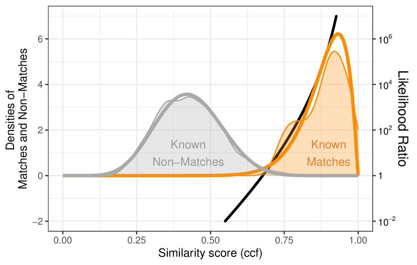
Figure 5: Densities for Known Match (KM) and Known Non-Match (KNM) pairs in terms of similarity (cross-correlation function) between pairs. For the KNM density, we averaged similarities across replicates. The thick curves are Beta distributions that fit the data and cross at 0.67. The likelihood ratio curve is shown as a function of the similarity score in black.

In Figure 5, we use this approach to compare the distribution of similarity scores for KMs and KNMs. For the KNM density, we group similarity scores by their sources and average across replicates. In other words, for the KNM density, we consider all possible combinations of 8 replicates for one source across 8 replicates for the other, resulting in 64 similarity scores for a pair of sources, and then we take the average over these 64 scores. For the KM density, we include all pairwise combinations of replicates from each source. We include the data from all three experiments.

We fit parametric (Beta) distributions on each curve. The parameters for Beta distributions are chosen such that the first moment and the second moment are matched with data. Figure 5 demonstrates the two density curves along with their fitted Beta distributions. Note that the parameters for Beta distributions are derived to match the first and second moment of the data. Specifically, we obtained that for the KM curve, $\alpha=15.7494,\beta=2.0665$ and for the KNM curve, $\alpha=8.5774,\beta=11.4628$. The curves are well separated, and they intersect around a similarity score (ccf) of 0.67.

The black line in Figure 5 shows the change in likelihood ratio as the similarity score increases. As a result, for any new pair of toolmark signals, we can calculate a LR that will indicate whether the evidence is more likely under the “same source” proposition or the “different source” proposition.

5.2 Method performance

5.2.1 Cross-validated performance

We use cross-validation to validate the algorithm, i.e., the classification between same-source and different-source pairs by using the threshold from where the KN and KNM densities intersect along the ccf similarity axis. Specifically, we split the data into two folds, one with all the marks made by the tools marked by even numbers and the other with all the marks made by tools with odd numbers. We train using the marks from experiment 1 and obtain a threshold. Then we use this threshold to classify between same-source and different-source pairs in the testing test. We calculate the sensitivity and specificity of our algorithm by comparing the predicted outcome with the ground truth (KM or KNM). We then repeat this procedure with the second fold, and average the sensitivity and specificity to obtain the cross-validated performance metrics.

Table 2 shows the cross-validated sensitivity and specificity of our procedure. From the table, it can be seen that as we expected, the in-sample performance is nearly perfect. Note that including the data from experiments 2 and 3 in the training of the algorithm yields the same performance metrics. This suggests that, at least for the data we collected, the angle and direction do not affect the classification performance of the algorithm.

Table 2: Algorithm performance.

	In-sample
Sensitivity	0.98
Specificity	0.96

5.2.2 Performance as a function of length

Sometimes practitioners have a very short striation mark from a tool, from a crime scene, and they need to know whether a candidate tool created this short mark. For example, the examiner may need to compare a short mark made by a slotted screwdriver on the edge of a surface, to longer test marks made by a candidate screwdriver. Another example is a thin wire that is cut with wire cutters – the mark on the wire can be quite short. We can test the performance of the method as the length of one of the marks decreases.

Intuitively, as the length of one of the signals decreases, there is less information in the signal. Thus, the signal becomes more similar to the marks made by other tools, and the false positive rate increases. In other words, in the extreme case, the signal is very short. Thus, it has very little information, and this means it could have been produced by any of the candidate tools.

Figures 6 show the specificity and sensitivity as functions of length, with decreasing length. That is, the performance of the algorithm as we shorten the length of one signal and compare it to a full-length signal. The sensitivity is not very informative – there seem to be no major changes in the true positive or false negative rates as signal length decreases.

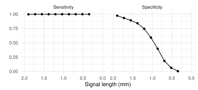
Figure 6: Performance as a function of length.

A specificity of 0.9, which corresponds to a 10% false positive rate, is reached at a signal length of about 1.5 mm. Once the signal length decreases further, there is not enough information to determine its source with any reasonable accuracy. At a signal length of just under 1 mm specificity drops to 50%, i.e. the accuracy of assessing whether a signal of that length matches a specific source is equal to a coin flip.

We see a similar dependence of accuracy on signal length in [Hare et al., 2017a]: at 37.5% of a land engraved area (corresponding to about $.375\times 2.2$ mm = 0.825 mm) specificity drops below 0.9 (for a sensitivity of about 0.7).

6 Discussion

Our method shows that it is possible to distinguish between same-source and different-source pairs of toolmarks reliably, and with a known measure of uncertainty. We present an objective method to perform forensic toolmark comparisons that presents results using likelihood ratios and addresses the problem of the “degrees of freedom”. We find that the changing the angle of attack (from 60 to 70 to 80 degrees with respect to the surface) and direction of mark generation (pulling and pushing) does not affect whether signals made by a source cluster together, or whether the algorithm classifies reliably. Our method has cross-validated sensitivity of 98% and specificity of 96%. This is very encouraging because it show that the method performs well even with consecutively manufactured tools, which are products of the same manufacturing process and thus one of the most difficult groups to classify correctly.

We found that very short signals, below 1.5 mm, in length cannot be compared reliably, even in this experimental setup where we have high-quality 3D data generated under controlled conditions. These results are particularly relevant for establishing error rates for comparisons with respect to the length of a signal.

For this experiment, we generated an original dataset of 3D toolmarks and their corresponding 2D signals, which is available for other researchers to use. We do not know how factors, such as angle of rotation, interaction of one tool with another as in wire cutters, tools that have strong class characteristics like serrated knives affect the classification performance of the algorithm out-of-sample. Although we must leave it for future work, it would be worthwhile to study the generalizability of this threshold to other tools and factors. Indeed, some methods have been trained on specific screwdrivers, there is evidence that they could be used to compare other tools as well [Baiker et al., 2014]. This is promising because it means that, for toolmark comparisons to be accurate and useful, it might only be necessary to train algorithms using a small number of tools. Collecting data from all the tools that could be used to commit a crime is practically impossible, especially as the number and types of tools grows over time. Further research is necessary to determine how much each type of tool generalizes to other types of tools.

The shift from subjective to objective comparison methods in pattern-matching forensic disciplines has the potential to improve consistency, allow for the demonstration of process validation, and have less uncertainty in conclusions, all of which can reduce errors in comparisons and, therefore, improve the criminal justice system.

7 Acknowledgments

This work was partially funded by the Center for Statistics and Applications in Forensic Evidence (CSAFE) through Cooperative Agreement 70NANB20H019 between NIST and Iowa State University, which includes activities carried out at Carnegie Mellon University, Duke University, University of California Irvine, University of Virginia, West Virginia University, University of Pennsylvania, Swarthmore College and University of Nebraska, Lincoln. We thank the National Institute of Standards and Technology for advising and contributing to the equipment. We also thank Danica Ommen and Federico Veneri Guarch for their guidance on dependencies in the data.

References

- [AFTE, 1998] AFTE (1998). The association of firearm and tool mark examiners: Theory of identification as it relates to toolmarks. AFTE Journal, 30(1):86–88.
- [Aitken and Taroni, 2004] Aitken, C. G. G. and Taroni, F. (2004). Statistics and the Evaluation of Evidence for Forensic Scientists. John Wiley and Sons, Ltd., West Sussex, UK.
- [Baiker et al., 2014] Baiker, M., Keereweer, I., Pieterman, R., Vermeij, E., van der Weerd, J., and Zoon, P. (2014). Quantitative comparison of striated toolmarks. Forensic Science International, 242:186–199.
- [Baiker et al., 2015] Baiker, M., Pieterman, R., and Zoon, P. (2015). Toolmark variability and quality depending on the fundamental parameters: angle of attack, toolmark depth and substrate material. Forensic Science International, 251:40–49.
- [Baiker-Sørensen et al., 2020] Baiker-Sørensen, M., Herlaar, K., Keereweer, I., Pauw-Vugts, P., and Visser, R. (2020). Interpol review of shoe and tool marks 2016-2019. Forensic Science International: Synergy, 2:521–539.
- [Baldwin et al., 2013] Baldwin, D., Birkett, J., Facey, O., and Rabey, G. (2013). The forensic examination and interpretation of tool marks. John Wiley & Sons, Hoboken, NJ.
- [Carriquiry et al., 2019] Carriquiry, A., Hofmann, H., Tai, X. H., and VanderPlas, S. (2019). Machine learning in forensic applications. Significance, 16(2):29–35.
- [Dodge, 1987] Dodge, Y. (1987). An introduction to l1-norm based statistical data analysis. Computational Statistics & Data Analysis, 5(4):239–253.
- [GelSight, 2023] GelSight (2023). Gelsightmobile usermanual 3.2. Technical report, GelSight, Cambridge, MA.
- [Hadler and Morris, 2018] Hadler, J. R. and Morris, M. D. (2018). An improved version of a tool mark comparison algorithm. Journal of Forensic Science, 63(3):849–855.
- [Hare et al., 2017a] Hare, E., Hofmann, H., and Carriquiry, A. (2017a). Algorithmic approaches to match degraded land impressions. Law, Probability and Risk, 16(4):203–221.
- [Hare et al., 2017b] Hare, E., Hofmann, H., and Carriquiry, A. (2017b). Automatic matching of bullet land impressions. The Annals of Applied Statistics, 11(4):2332–2356.
- [Hofmann et al., 2022] Hofmann, H., Vanderplas, S., Ju, W., and Krishnan, G. (2022). bulletxtrctr: Automatic Matching of Bullet Striae. R package version 0.2.0.9000.
- [Kafadar, 2019] Kafadar, K. (2019). The need for objective measures in forensic evidence. Significance, 16(2):16–20.
- [Kaufman and Rousseeuw, 2009] Kaufman, L. and Rousseeuw, P. J. (2009). Finding groups in data: an introduction to cluster analysis. John Wiley & Sons.
- [Lock and Morris, 2013] Lock, A. B. and Morris, M. D. (2013). Significance of angle in the statistical comparison of forensic tool marks. Technometrics, 55(4):548–561.
- [Macziewski et al., 2017] Macziewski, C., Spotts, R., and Chumbley, S. (2017). Validation of toolmark comparisons made at different vertical and horizontal angles. Journal of Forensic Sciences, 62(3):612–618.
- [M.S. et al., 2015] M.S., R. S., Chumbley, L. S., Ekstrand, L., Zhang, S., and Kreiser, J. (2015). Angular determination of toolmarks using a computer-generated virtual tool. Journal of Forensic Sciences, 60(4):878–884.
- [Nichols, 1997] Nichols, R. (1997). Firearm and toolmark identification criteria: review of literature. Journal of Forensic Sciences, 42(3):466–474.
- [Nichols, 2003] Nichols, R. (2003). Firearm and toolmark identification criteria: a review of the literature, part ii. Journal of Forensic Sciences, 48(2):318–327.