A new numerical technique based on Chelyshkov polynomials for solving two-dimensional stochastic Itô-Volterra Fredholm integral equation

Abstract

In this paper, a two-dimensional operational matrix method based on Chelyshkov polynomials is implemented to numerically solve the two-dimensional stochastic Itô-Volterra Fredholm integral equations. These equations arise in several problems such as an exponential population growth model with several independent white noise sources. In this paper a new stochastic operational matrix has been derived first time ever by using Chelyshkov polynomials. After that, the operational matrices are used to transform the Itô-Volterra Fredholm integral equation into a system of linear algebraic equations by using Newton cotes nodes as collocation point that can be easily solved. Furthermore, the convergence and error bound of the suggested method are well established. In order to illustrate the effectiveness, plausibility, reliability, and applicability of the existing technique, two typical examples have been presented.

Keywords: Stochastic Itô-Volterra Fredholm integral equation; Itô integral; Brownian motion; Chelyshkov polynomial; Collocation method; Error analysis; Convergence.

MSC: 60H20, 45D05, 65R20, 45B05.

1 Introduction

Many problems originating in mathematical physics can be solved using several types of integral equations, such as Fredholm IEs [1], Volterra integral equations (IEs) [2, 3], integro-differential equations [4, 5], Volterra-Fredholm IEs [6], , fractional differential equations [7] etc. There has been a lot of interest in studying mathematical models utilising the Itô integral, particularly in science and engineering. Due to the fact that stochastic processes arise in several real problems. including control systems [8], biological population growth [9], and challenges in physics, chemistry, and biology [10]. Functional equations with deterministic and stochastic properties are fundamental modelling tools for a wide range of characteristics. It can be difficult and time-consuming to explicitly solve IEs, stochastic integral equations (SIEs), nonlinear stochastic differential equations by variable fractional Brownian motion [11] and stochastic fractional integro-differential equations (SFIDEs) [12]. So there are several different numerical algorithms established to solve deterministic IEs or SIEs. For example: second-order Runge-Kutta method [13], Bernoullis approximation [14], cubic B-spline approximation [15], block pulse approximation [16], moving least squares method [17], radial basis functions [18], Bernstien polynomials [19], shifted Legendre polynomials [20], Shifted Jacobi operational matrix [21], meshless local discrete Galerkin scheme [22], and various others techniques have been employed to solve different types of integral equations.

The main focus of this work is to determine the numerical solution of 2-D stochastic Itô-Volterra Fredholm integral equation (SIVFIE) given by:

$$f(u,v) =g(u,v)+\int_{0}^{1}\int_{0}^{1}\kappa_{1}(u,v,s,t)f(s,t)dtds+\int_{0}^{u}\int_{0}^{v}\kappa_{2}(u,v,s,t)f(s,t)dtds$$

$$+\int_{0}^{u}\int_{0}^{v}\kappa_{3}(u,v,s,t)f(s,t)dB(t)dB(s),\quad(u,v)\in[0,1]\times[0,1].$$ (1.1)

In the given equation, $g(u,v$) and $\kappa_{i}(u,v,s,t)$ for $i=1,2$ and 3 are known smooth functions and $f(u,v)$ is an unknown function, that needs to be determined. This is referred to as the solution of 2-D SIVFIE. Brownian motion is defined as $\{B(t),t\geq 0\}$ and $\int_{0}^{u}\int_{0}^{v}\kappa_{3}(u,v,s,t)f(s,t)dB(t)dB(s)$ is 2-D Itô integral.

The primary goal of this work is to find the solution of 2-D SIVFIE. These equations are important in a variety of applied fields, including biology, epidemiology, chemistry, and mechanics. It can be difficult and time-consuming to solve SFIDE explicitly. Therefore, in this case, the operational matrix approach is used to find the numerical solutions of these equations. In this study, a novel stochastic operational matrix is developed by using Chelyshkov polynomials. The suggested approach works well and is efficient and reliable.

In this article, the 2-D SIVFIE (eq.(1.1)) is solved by using Chelyshkov polynomials [23, 24]. Eq. (1.1) has been reduced to an algebraic system of equations by using derived operational matrices for product, integral and stochastic along with the suitable collocation points. The resultant equations can be easily solved to get the desired approximate solution.

This manuscript is organized as follows:
Section 2 introduced fundamental concepts such as Brownian motion and the properties of Chelyshkov polynomials (CPs). Operational matrices (OMs) for products, integrals, and stochastic integrals have been derived in Section 3. In Section 4, a summary of the details of the collocation technique is presented, and the 2-D SIVFIE problem is solved by using the proposed two-dimensional operational matrix method. Theorems related to convergence analysis and error estimation are discussed in Section 5. Section 6 demonstrates the efficacy and applicability of the suggested numerical approach by considering two typical problems, and a brief summary is described in Section 7.

2 Premilaries

In this part, the properties of CPs are discussed together with some fundamental stochastic calculus concepts.

2.1 Stochastic calculus

Definition 1 ( Itô Integral [25]). Consider $\mathcal{V}=\mathcal{V}(X,Y)$ be the class of functions $h(\vartheta,\varpi):[0,\infty)\times\Omega\rightarrow\mathbb{R}$ and $h\in\mathcal{V}(X,Y)$. Thus, the definition of the Itô integral of $h$ is given by

$$\int_{X}^{Y}h(\vartheta,\varpi)dB_{\vartheta}(\varpi)=\lim_{n\to\infty}\int_{X}^{Y}\psi_{n}(\vartheta,\varpi)dB_{\vartheta}(\varpi)\quad(\lim in\,L^{2}(\mathbb{P})),$$

where $\{\psi_{n}\}$ is a sequence involving the elementary functions, satisfying the conditions given as:

$$E\left[\int_{X}^{Y}(h(\vartheta,\varpi)-\psi_{n}(\vartheta,\varpi))^{2}d\vartheta,\right]\rightarrow 0\,as\,n\rightarrow\infty.$$

Theorem 2.1.1 ( The Itô isometry [25]). Let $h\in\mathcal{V}(X,Y)$, be elementary and bounded functions. Then

$$E\left[\left(\int_{X}^{Y}h(\vartheta,\varpi)dB_{\vartheta}(\varpi)\right)^{2}\right]=E\left[\int_{X}^{Y}h^{2}(\vartheta,\varpi)d\vartheta\right].$$

2.2 Chelyshkov polynomial and its properties

Chelyshkov recently introduced orthogonal polynomial sequences in the interval [0, 1] with the weight function 1. These polynomials are described as follows:

$$\psi_{i}(s)=\sum_{k=0}^{N-i}(-1)^{k}\binom{N-i}{k}\binom{N+k+i+1}{N-i}s^{k+i},\quad 0\leq i\leq N.$$

An $(N+1)$ set of the orthonormal Chelyshkov polynomials (OCPs) is defined over $[0,1]$ by

$$\psi^{*}_{i}(s)=\sqrt{2i+1}\sum_{k=0}^{N-i}(-1)^{k}\binom{N-i}{k}\binom{N+k+i+1}{N-i}s^{k+i},\quad 0\leq i\leq N.$$ (2.1)

The orthonormal property is given by

$\int_{0}^{1}\psi^{*}_{i}(s)\psi^{*}_{j}(s)ds=\begin{cases}1&i=j\\ 0&i\mathrel{\vphantom{|}\mathchoice{\ooalign{$\displaystyle|$\cr$\displaystyle=$\cr}}{\ooalign{$\textstyle|$\cr$\textstyle=$\cr}}{\ooalign{$\scriptstyle|$\cr$\scriptstyle=$\cr}}{\ooalign{$\scriptscriptstyle|$\cr$\scriptscriptstyle=$\cr}}}j\end{cases}.$

These polynomials are connected to the following set of Jacobi polynomials:

$$\psi_{i}(s)=(-1)^{N-i}s^{i}P^{0,2i+1}_{N-i}(2s-1),\quad i=0,1,2...,N.$$

A set of 1-D basis vector is defined as follows:

$$\Psi(s)=[\psi^{*}_{0}(s),\psi^{*}_{1}(s),...,\psi^{*}_{N}(s)]^{T}.$$

The definition of a 2-D basis polynomial of order $m,n$ is given below.

$$\psi^{*}_{m,n}(s,t)=\psi^{*}_{m}(s)\psi^{*}_{n}(t)\quad m,n=0,1,2,...$$

The 2-D basis vector is defined as follows:

$$\Psi(s,t)=[\psi^{*}_{0,0}(s,t),\psi^{*}_{0,1}(s,t),...,\psi^{*}_{0,N}(s,t),...,\psi^{*}_{N,0}(s,t),\psi^{*}_{N,1}(s,t),...,\psi^{*}_{N,N}(s,t)]^{T},$$

Equivalently,

$$\Psi(s,t)=\Psi(s)\otimes\Psi(t).$$

where $\Psi(s)$ and $\Psi(t)$ are 1-D basis vectors and $\otimes$ is the kronecker product.

Now using eq. (2.1) we obtain

$$\Psi(s)=HT_{N}(s),$$ (2.2)

where

$$T_{N}(s)=[1,s,...,s^{N}]^{T},$$

and $H_{(N+1)\times(N+1)}$ is determined by

$H=\begin{pmatrix}(-1)^{0}\binom{N}{0}\binom{N+1}{N}&(-1)^{1}\binom{N}{1}\binom{N+2}{N}&\dots&(-1)^{N}\binom{N}{N}\binom{2N+1}{N}\\ 0&(-1)^{0}\binom{N-1}{0}\binom{N+2}{N-1}&\dots&(-1)^{N-1}\binom{N-1}{N-1}\binom{N+1}{N-1}\\ \vdots&\vdots&\ddots&\vdots\\ 0&0&\dots&(-1)^{0}\binom{N-N}{0}\binom{2N+1}{0}\end{pmatrix}$,

where $H$ is a nonzero upper triangular matrix. Thus, this matrix is non singular and hence $H^{-1}$ exists.

Therefore,

$$T_{N}(s)=H^{-1}\Psi(s)$$

2.3 Function approximation by OCPs

Every two-variable function $y(s,t)$ in the range $[0,1]\times[0,1]$ can be approximated as follows: :

$$y(s,t)\simeq y_{N}(s,t)=\sum_{i=0}^{N}\sum_{j=0}^{N}\psi^{*}_{i}(s)w^{*}_{ij}\psi^{*}_{j}(t)=\Psi^{T}(s)W\Psi(t),$$

where $W=[w^{*}_{ij}]_{(N+1)\times(N+1)}$ and $w^{*}_{ij}$ is described as:

$$w^{*}_{ij}=\int_{0}^{1}\int_{0}^{1}\psi^{*}_{i}(s)y(s,t)\psi^{*}_{j}(t)dtds,\hskip 28.45274pti,j=0,1,...,N.$$

It is simple to demonstrate by calculations that:

$$y(s,t)\simeq W^{*T}(\Psi(s)\otimes\Psi(t))=W^{*T}\Psi(s,t),$$

where $W^{*}_{(N+1)^{2}\times 1}$ is a coefficient vector which is defined as follows:

$W^{*}=\left[w^{*}_{00},w^{*}_{01},...,w^{*}_{0N},w^{*}_{10},w^{*}_{11},...,w^{*}_{1N},...,w^{*}_{N0},w^{*}_{N1},...,w^{*}_{NN}\right]^{T}.$

Consequently, an arbitrary function $\kappa(u,v,s,t)$ is approximated by 2-D OCPs as:

$$\kappa(u,v,s,t)\simeq\Psi^{T}(u,v)K\Psi(s,t)=\Psi^{T}(s,t)K^{T}\Psi(u,v),$$ (2.3)

where $K_{(N+1)^{2}\times(N+1)^{2}}$ is given by

$$K=\int_{0}^{1}\int_{0}^{1}\Psi(u,v)\left(\int_{0}^{1}\int_{0}^{1}\kappa(u,v,s,t)\Psi^{T}(s,t)dtds\right)dvdu.$$

3 OMs for OCPs

3.1 OM for product

In this analysis, OM for product is derived.

$$\Psi(s,t)\Psi^{T}(s,t)F\simeq\hat{F}\Psi(s,t),$$

where $\hat{F}_{(N+1)^{2}\times(N+1)^{2}}$ is a product OM which is determined by using orthonormal property of CPs.

$$\hat{F}=\int_{0}^{1}\int_{0}^{1}\left(\Psi(s,t)\Psi^{T}(s,t)F\right)\Psi^{T}(s,t)dtds.$$

3.2 OM for integral

The integration of 2-D vector $\Psi(s,t)$ can be defined as follows:

$$\int_{0}^{u}\int_{0}^{v}\Psi(s,t)dtds\simeq\hat{P_{I}}\Psi(s,t),$$

where $\hat{P_{I}}_{(N+1)^{2}\times(N+1)^{2}}$ is a product OM which is determined by using orthonormal property of CPs.

$$\hat{P_{I}}=\int_{0}^{1}\int_{0}^{1}\left(\int_{0}^{u}\int_{0}^{v}\Psi(s,t)dtds\right)\Psi^{T}(s,t)dtds.$$

3.3 Stochastic operational matrix

Here the Itô integral of vector $\Psi(s)$ can be approximated in terms of stochastic OM as follows:

$$\int_{0}^{u}\Psi(s)dB(s)\simeq Q_{s}\Psi(u),$$

and for 2-D vector it is defined as

$$\int_{0}^{u}\int_{0}^{v}\Psi(s,t)dB(t)dB(s)\simeq\hat{Q_{s}}\Psi(u,v),$$ (3.1)

where ${Q_{s}}_{(N+1)\times(N+1)}$ is a stochastic OM and $\hat{Q_{s}}_{(N+1)^{2}\times(N+1)^{2}}$ is a stochastic OM.

3.3.1 Calculation for $\hat{Q_{s}}$ matrix:

From eq. (2.2)

$\Psi(s)=HT_{N}(s)$.

Now,

$$\int_{0}^{u}\Psi(s)dB(s)=\int_{0}^{u}HT_{N}(s)dB(s)=H\int_{0}^{u}T_{N}(s)dB(s),$$ (3.2)

Again,

$$\int_{0}^{u}T_{N}(s)dB(s)=\left[\int_{0}^{u}dB(s),\int_{0}^{u}sdB(s),...,\int_{0}^{u}s^{N}dB(s)\right]^{T}.$$

Thus,

$$\begin{bmatrix}\int_{0}^{u}dB(s)\\ \int_{0}^{u}sdB(s)\\ \int_{0}^{u}s^{2}dB(s)\\ \vdots\\ \int_{0}^{u}s^{N}dB(s)\end{bmatrix}=\begin{bmatrix}\ B(u)\\ \ uB(u)-\int_{0}^{u}B(s)ds\\ \ u^{2}B(u)-2\int_{0}^{u}sB(s)ds\\ \vdots\\ \ u^{N}B(u)-N\int_{0}^{u}s^{(N-1)}B(s)ds\end{bmatrix}\\ =R_{N}(u)=[r_{i}]_{(m+1)\times 1},$$ (3.3)

where

$r_{i}=u^{i}B(u)-i\int_{0}^{u}s^{i-1}B(s)ds$, $i=0,1,2,...,N$.

Approximate the integrals in eq. (3.3) by using the Simpson $\dfrac{1}{3}$ rule yields

$$r_{i}=\left(1-\dfrac{i}{6}\right)u^{i}B(u)-\dfrac{i}{3\times 2^{i-2}}u^{i}B\left(\dfrac{u}{2}\right),\quad i=0,1,2,...,N.$$ (3.4)

Now, in eq. (3.4), $B\left(\dfrac{u}{2}\right),B(u)$ are approximated by $B(0.25)$ and $B(0.5)$, respectively.

Thus,

$$\int_{0}^{u}T_{N}(s)dB(s)\simeq\begin{bmatrix}B(0.5)&0&\dots&0\\ 0&\frac{5}{6}B(0.5)-\frac{2}{3}B(0.25)&\dots&0\\ \vdots&\vdots&\ddots&\vdots\\ 0&0&\dots&\left(1-\frac{N}{6}\right)B(0.5)-\dfrac{N}{3\times 2^{N-2}}B(0.25)\end{bmatrix}\begin{bmatrix}1\\ u\\ \vdots\\ u^{N}\end{bmatrix}=\Phi_{s}T_{N}(u).$$ (3.5)

Now using eq. (3.2) and (3.5), yields

$$\int_{0}^{u}\Psi(s)dB(s)=H\Phi_{s}T_{N}(u)=H\Phi_{s}H^{-1}\Psi(u)=Q_{s}\Psi(u),$$

Hence,

$$Q_{s}=H\Phi_{s}H^{-1}.$$

Now, in eq. (3.1) $\hat{Q_{s}}$ is determined by

$$\hat{Q_{s}}=Q_{s}\otimes Q_{s}.$$

4 Numerical method

In this analysis, eq. (1.1) has been solved by using the new proposed two-dimensional operational matrix method which is based on two-dimensional Chelyshkov polynomials. To implement this, the functions $f(u,v)$, $g(u,v$) and $\kappa_{i}(u,v,s,t)$ for $i=1,2$ and 3 are approximated based on a 2-D basis vector, such that:

$$f(u,v)\simeq f_{N}(u,v)=\Psi^{T}(u,v)F.$$ (4.1)

$$g(u,v)\simeq g_{N}(u,v)=\Psi^{T}(u,v)G.$$ (4.2)

$$\kappa_{i}(u,v,s,t)\simeq\Psi^{T}(u,v)K_{i}\Psi(s,t),\hskip 14.22636pti=1,2,3,$$ (4.3)

where $F=[f_{ij}]_{(N+1)^{2}\times 1}$ and $G=[\sigma_{ij}]_{(N+1)^{2}\times 1}$ are provided by

$$F=\left[f_{00},f_{01},...,f_{0N},f_{10},f_{11},...,f_{1N},...,f_{N0},f_{N1},...,f_{NN}\right]^{T},$$

$$G=\left[\sigma_{00},\sigma_{01},...,\sigma_{0N},\sigma_{10},\sigma_{11},...,\sigma_{1N},...,\sigma_{N0},\sigma_{N1},...,\sigma_{NN}\right]^{T},$$

where $f_{ij}$ and $\sigma_{ij}$ are defined as follows:

$$f_{ij}=\int_{0}^{1}\int_{0}^{1}\psi^{*}_{i}(u)f(u,v)\psi^{*}_{j}(v)dvdu,$$

$$\sigma_{ij}=\int_{0}^{1}\int_{0}^{1}\psi^{*}_{i}(u)g(u,v)\psi^{*}_{j}(v)dvdu,$$

and $K_{i}$ is a kernal matrix given by eq. (2.3).

Now, the integrals in eq. (1.1) are approximated as follows:

For Fredholm integral:

$$\int_{0}^{1}\int_{0}^{1}\kappa_{1}(u,v,s,t)f(s,t)dtds =\int_{0}^{1}\int_{0}^{1}\Psi^{T}(u,v)K_{1}\Psi(s,t)\Psi^{T}(s,t)Fdtds$$

$$=\Psi^{T}(u,v)K_{1}\int_{0}^{1}\int_{0}^{1}\Psi(s,t)\Psi^{T}(s,t)dtdsF$$ (4.4)

$$=\Psi^{T}(u,v)K_{1}\hat{I}F,$$

where $\hat{I}$ is defined by

$$\hat{I}=\int_{0}^{1}\int_{0}^{1}\Psi(s,t)\Psi^{T}(s,t)dtds.$$

For Volterra integral:

$$\int_{0}^{u}\int_{0}^{v}\kappa_{2}(u,v,s,t)f(s,t)dtds =\int_{0}^{u}\int_{0}^{v}\Psi^{T}(u,v)K_{2}\Psi(s,t)\Psi^{T}(s,t)Fdtds$$

$$=\Psi^{T}(u,v)K_{2}\int_{0}^{u}\int_{0}^{v}\Psi(s,t)\Psi^{T}(s,t)Fdtds$$

$$=\Psi^{T}(u,v)K_{2}\int_{0}^{u}\int_{0}^{v}\hat{F}\Psi(s,t)dtds$$ (4.5)

$$=\Psi^{T}(u,v)K_{2}\hat{F}\int_{0}^{u}\int_{0}^{v}\Psi(s,t)dtds$$

$$=\Psi^{T}(u,v)K_{2}\hat{F}\hat{P_{I}}\Psi(u,v).$$

For Itô integral:

$$\int_{0}^{u}\int_{0}^{v}\kappa_{3}(u,v,s,t)f(s,t)dB(t)dB(s) =\int_{0}^{u}\int_{0}^{v}\Psi^{T}(u,v)K_{3}\Psi(s,t)\Psi^{T}(s,t)FdB(t)dB(s)$$

$$=\Psi^{T}(u,v)K_{3}\int_{0}^{u}\int_{0}^{v}\Psi(s,t)\Psi^{T}(s,t)FdB(t)dB(s)$$

$$=\Psi^{T}(u,v)K_{3}\int_{0}^{u}\int_{0}^{v}\hat{F}\Psi(s,t)dB(t)dB(s)$$ (4.6)

$$=\Psi^{T}(u,v)K_{3}\hat{F}\int_{0}^{u}\int_{0}^{v}\Psi(s,t)dB(t)dB(s)$$

$$=\Psi^{T}(u,v)K_{3}\hat{F}\hat{Q_{s}}\Psi(u,v).$$

Now, substituting eqs. (4.1)-(4.6) in eq. (1.1).

$$\Psi^{T}(u,v)F=\Psi^{T}(u,v)G+\Psi^{T}(u,v)K_{1}\hat{I}F+\Psi^{T}(u,v)K_{2}\hat{F}\hat{P_{I}}\Psi(u,v)+\Psi^{T}(u,v)K_{3}\hat{F}\hat{Q_{s}}\Psi(u,v).$$ (4.7)

Collocating eq. (4.7) at the Newton-Cotes collocation points provided by $(u_{i},v_{j})=\left(\dfrac{2i-1}{2(N+1)},\dfrac{2j-1}{2(N+1)}\right)$, $i,j=1,2,...,N+1$ generates a system of algebraic equations. The coefficient vector $F$ is obtained by solving this set of algebraic equations. This linear system contains $(N+1)^{2}$ equations which can be solved for $(N+1)^{2}$ unknown coefficients using suitable numerical technique. After that the final approximate solution is obtained by the equation $f(u,v)=\Psi^{T}(u,v)F$.

5 Error Estimate and Convergence Analysis

5.1 Error analysis:

Consider the following 2-D SIVFIE:

$$f(u,v) =g(u,v)+\iint\limits_{\Omega}\kappa_{1}(u,v,s,t)f(s,t)dtds+\iint\limits_{\mathcal{D}}\kappa_{2}(u,v,s,t)f(s,t)dtds$$

$$+\iint\limits_{\mathcal{D}}\kappa_{3}(u,v,s,t)f(s,t)dB(t)dB(s),$$ (5.1)

where $\Omega\equiv[0,1]\times[0,1]$ and $\mathcal{D}\equiv[0,u]\times[0,v]\subset\Omega.$

Let us introduce the following integral operators $I_{1},I_{2}$ and $I_{3}$ respectively.

$$(I_{1}f)(u,v)=\iint\limits_{\Omega}\kappa_{1}(u,v,s,t)f(s,t)dtds,$$

$$(I_{2}f)(u,v)=\iint\limits_{\mathcal{D}}\kappa_{2}(u,v,s,t)f(s,t)dtds,$$

$$\hskip 28.45274pt(I_{3}f)(u,v)=\iint\limits_{\mathcal{D}}\kappa_{3}(u,v,s,t)f(s,t)dB(t)dB(s),$$

Now, eq. (5.1) can be rewritten in the following form using the above operators.

$$f=g+I_{1}f+I_{2}f+I_{3}f.$$ (5.2)

Suppose $f_{N,N}(u,v)=F^{T}\Psi(u,v)$ be the 2-D operational matrix method(OMM) approximate solution of eq. (5.1).

Let $\Pi_{N,N}(\Omega)$, where $\Omega\equiv[0,1]\times[0,1]$ is the space of polynomials of degree $\leq N$ in $u$ and degree $\leq N$ in $v$. Then the functions $\{\psi_{ij}(u,v)\}$ where $i=0,1,2,...,N$ ; $j=0,1,2,...,N$ form an orthonormal basis for $\Pi_{N,N}(\Omega)$,

where

$\Pi_{N,N}(\Omega)=Span\{\psi_{ij}(u,v):i=0,1,...,N;j=0,1,...,N\}$.

If

$f_{N,N}(u,v)\in\Pi_{N,N}(\Omega)$,

then

$$f_{N,N}(u,v)=\sum^{N}_{i=0}\sum^{N}_{j=0}f_{ij}\psi_{ij}(u,v)=F^{T}\Psi(u,v)=\Psi^{T}(u,v)F,$$

where

$\Psi^{T}(u,v)=[\psi_{0,0}(u,v),\psi_{0,1}(u,v),...,\psi_{0,N}(u,v),...,\psi_{N,0}(u,v),\psi_{N,1}(u,v),...,\psi_{N,N}(u,v)]$,

and $F$ is the $(N+1)^{2}\times 1$ -dimensional coefficient vector defined by the following relation.

$F=\langle f_{N,N}(u,v),\Psi(u,v)\rangle$.

Let us define the approximate operators as follows:

$$(I_{1N}f)(u,v):=\Psi^{T}(u,v)K_{1}F$$

$$(I_{2N}f)(u,v):=\Psi^{T}(u,v)K_{2}\hat{F}\hat{P_{I}}\Psi(u,v)$$

$$(I_{3N}f)(u,v):=\Psi^{T}(u,v)K_{3}\hat{F}\hat{Q_{s}}\Psi(u,v).$$

The following set of collocation points

$\chi=\{(u_{i},v_{i})\}^{N}_{i=0}\subset\mathcal{D}$,

and a collocation projection operator $\mathcal{P}_{N,N}$ on this set have been considered.

Now, eq. (5.1) can be written as

$$\Psi^{T}(u_{j},v_{j})F=\Psi^{T}(u_{j},v_{j})G+\Psi^{T}(u_{j},v_{j})K_{1}F+\Psi^{T}(u_{j},v_{j})K_{2}\hat{F}\hat{P_{I}}\Psi(u_{j},v_{j})+\Psi^{T}(u_{j},v_{j})K_{3}\hat{F}\hat{Q_{s}}\Psi(u_{j},v_{j}),$$ (5.3)

$j=0,1,2,...,N.$
Now, if

$f_{N,N}\in\Pi_{N,N}(\mathcal{D})$,

then,

$P_{N,N}f_{N,N}=f_{N,N}$,

where $P_{N,N}f_{N,N}$ stands for the interpolation polynomial of $f_{N,N}$ at the interpolating points $(s_{j},t_{j})$, $j=0,1,2,...,N.$

For sufficiently large integer $N$, eq. (5.3) can be rewritten as follows:

$$f_{N,N}=\mathcal{P}_{N,N}g+\mathcal{P}_{N,N}I_{1N}f_{N,N}+\mathcal{P}_{N,N}I_{2N}f_{N,N}+\mathcal{P}_{N,N}I_{3N}f_{N,N},$$

whence

$$(I-\mathcal{P}_{N,N}I_{1N}-\mathcal{P}_{N,N}I_{2N}-\mathcal{P}_{N,N}I_{3N})f_{N,N}=\mathcal{P}_{N,N}g,$$ (5.4)

where $I$ is the identity operator.

Then from eq. (5.4), we obtain,

$$(I-I_{1N}\mathcal{P}_{N,N}-I_{2N}\mathcal{P}_{N,N}-I_{3N}\mathcal{P}_{N,N})f_{N,N}=g.$$ (5.5)

Theorem 5.1.1: Assume that
$(I-I_{1}-I_{2}-I_{3})$ is a bijective mapping on $C(\mathcal{D})$. Also the sequence of bounded linear operators $I_{1},I_{2}$ and $I_{3}$ exists such that

$$\lim_{N\to\infty}||I_{1}+I_{2}+I_{3}-I_{1N}\mathcal{P}_{N,N}-I_{2N}\mathcal{P}_{N,N}-I_{3N}\mathcal{P}_{N,N}||=0,$$ (5.6)

then the operator $(I-I_{1N}\mathcal{P}_{N,N}-I_{2N}\mathcal{P}_{N,N}-I_{3N}\mathcal{P}_{N,N})^{-1}$ for sufficiently large $N$, (say $N\geq m$ ) exists, and is bounded, Also the error bound is given by

$$||f-f_{N,N}|| \leq||(I-I_{1N}\mathcal{P}_{N,N}-I_{2N}\mathcal{P}_{N,N}-I_{3N}\mathcal{P}_{N,N})^{-1}||$$

$$\hskip 14.22636pt\times||I_{1}f-I_{1N}\mathcal{P}_{N,N}f+I_{2}f-I_{2N}\mathcal{P}_{N,N}f+I_{3}f-I_{3N}\mathcal{P}_{N,N}f||,$$

where

$$||(I-I_{1N}\mathcal{P}_{N,N}-I_{2N}\mathcal{P}_{N,N}-I_{3N}\mathcal{P}_{N,N})^{-1}||$$

$$\leq\frac{||(I-I_{1}-I_{2}-I_{3})^{-1}||}{(1-||(I-I_{1}-I_{2}-I_{3})^{-1}||\times||I_{1}+I_{2}+I_{3}-I_{1N}\mathcal{P}_{N,N}-I_{2N}\mathcal{P}_{N,N}-I_{3N}\mathcal{P}_{N,N}||)}.$$ (5.7)

Proof: Let us start with the following equation

$I-I_{1N}\mathcal{P}_{N,N}-I_{2N}\mathcal{P}_{N,N}-I_{3N}\mathcal{P}_{N,N}$

$$=(I-I_{1}-I_{2}-I_{3})[I+(I-I_{1}-I_{2}-I_{3})^{-1}\times(I_{1}+I_{2}+I_{3}-I_{1N}\mathcal{P}_{N,N}-I_{2N}\mathcal{P}_{N,N}-I_{3N}\mathcal{P}_{N,N})].$$ (5.8)

Now using eq. (5.6) in the hypothesis of theorem statement. Infact, we can find $m$ such that

$$||I_{1}+I_{2}+I_{3}-I_{1N}\mathcal{P}_{N,N}-I_{2N}\mathcal{P}_{N,N}-I_{3N}\mathcal{P}_{N,N}||<\dfrac{1}{||(I-I_{1}-I_{2}-I_{3})^{-1}||},N\geq m,$$ (5.9)

using reverse triangle inequality and eq. (5.8), it can be easily prove that,

$$||(I+(I-I_{1}-I_{2}-I_{3})^{-1}\times(I_{1}+I_{2}+I_{3}-I_{1N}\mathcal{P}_{N,N}-I_{2N}\mathcal{P}_{N,N}-I_{3N}\mathcal{P}_{N,N}))^{-1}||$$

$$\leq\dfrac{1}{1-||(I-I_{1}-I_{2}-I_{3})^{-1}||\times||I_{1}+I_{2}+I_{3}-I_{1N}\mathcal{P}_{N,N}-I_{2N}\mathcal{P}_{N,N}-I_{3N}\mathcal{P}_{N,N}||}.$$ (5.10)

Using eqs. (5.8), (5.9) and (5.10), we can obtain

$$||(I-I_{1N}\mathcal{P}_{N,N}-I_{2N}\mathcal{P}_{N,N}-I_{3N}\mathcal{P}_{N,N})^{-1}||$$

$$=||(I+(I-I_{1}-I_{2}-I_{3})^{-1}\times(I_{1}+I_{2}+I_{3}-I_{1N}\mathcal{P}_{N,N}-I_{2N}\mathcal{P}_{N,N}-I_{3N}\mathcal{P}_{N,N}))^{-1}||$$

$$\hskip 14.22636pt\times||(I-I_{1}-I_{2}-I_{3})^{-1}||$$

$$\leq\dfrac{||(I-I_{1}-I_{2}-I_{3})^{-1}||}{1-||(I-I_{1}-I_{2}-I_{3})^{-1}||\times||I_{1}+I_{2}+I_{3}-I_{1N}\mathcal{P}_{N,N}-I_{2N}\mathcal{P}_{N,N}-I_{3N}\mathcal{P}_{N,N}||}.$$

Thus, we have proved the existance of bound $(I-I_{1N}\mathcal{P}_{N,N}-I_{2N}\mathcal{P}_{N,N}-I_{3N}\mathcal{P}_{N,N})^{-1}$ and the bound is given by eq. (5.7).

Now using eq. (5.2) and (5.5), we have

$$||f-f_{N,N}|| =||(I-I_{1}-I_{2}-I_{3})^{-1}g-(I-I_{1N}\mathcal{P}_{N,N}-I_{2N}\mathcal{P}_{N,N}-I_{3N}\mathcal{P}_{N,N})^{-1}g||$$

$$=||(I-I_{1N}\mathcal{P}_{N,N}-I_{2N}\mathcal{P}_{N,N}-I_{3N}\mathcal{P}_{N,N})^{-1}$$

$$\hskip 14.22636pt\times(I_{1}+I_{2}+I_{3}-I_{1N}\mathcal{P}_{N,N}-I_{2N}\mathcal{P}_{N,N}-I_{3N}\mathcal{P}_{N,N})\times(I-I_{1}-I_{2}-I_{3})^{-1}g||$$

Therefore using eq. (5.2), we get

$$||f-f_{N,N}|| \leq||(I-I_{1N}\mathcal{P}_{N,N}-I_{2N}\mathcal{P}_{N,N}-I_{3N}\mathcal{P}_{N,N})^{-1}||$$

$$\hskip 14.22636pt\times||I_{1}f-I_{1N}\mathcal{P}_{N,N}f+I_{2}f-I_{2N}\mathcal{P}_{N,N}f+I_{3}f-I_{3N}\mathcal{P}_{N,N}f||.$$

$\blacksquare$

5.2 Convergence analysis:

Theorem 5.2.1: Consider the assumption of Theorem 5.1.1 and suppose $f$ and $f_{N,N}$ be the exact and approximate solution of eq. (5.1).

If

$L_{1}=Sup||(I-I_{1N}\mathcal{P}_{N,N}-I_{2N}\mathcal{P}_{N,N}-I_{3N}\mathcal{P}_{N,N})^{-1}||<\infty$,

$L_{I_{1}}=Sup||I_{1N}||<\infty$,

$L_{I_{2}}=Sup||I_{2N}||<\infty$,

$L_{I_{3}}=Sup||I_{3N}||<\infty$,

and $L_{\mathcal{P}}=Sup||\mathcal{P}_{N,N}||<\infty$, then $||f-f_{N,N}||\to 0$ as $N\to\infty.$

Proof: From Theorem 5.1.1, we have

$$||f-f_{N,N}|| \leq||(I-I_{1N}\mathcal{P}_{N,N}-I_{2N}\mathcal{P}_{N,N}-I_{3N}\mathcal{P}_{N,N})^{-1}||\times||I_{1}f-I_{1N}\mathcal{P}_{N,N}f+I_{2}f-I_{2N}\mathcal{P}_{N,N}f$$

$$\hskip 14.22636pt+I_{3}f-I_{3N}\mathcal{P}_{N,N}f||$$

$$\leq L_{1}(||I_{1}f-I_{1N}f||+||I_{1N}(f-\mathcal{P}_{N,N}f)||+||I_{2}f-I_{2N}f||+||I_{2N}(f-\mathcal{P}_{N,N}f)||$$

$$\hskip 14.22636pt+||I_{3}f-I_{3N}f||+||I_{3N}(f-\mathcal{P}_{N,N}f)||),$$

Thus, we obtain

$||f-f_{N,N}||\leq L_{1}(||I_{1}f-I_{1N}f||+||I_{2}f-I_{2N}f||+||I_{3}f-I_{3N}f||+(L_{I_{1}}+L_{I_{2}}+L_{I_{3}})||f-\mathcal{P}_{N,N}f||).$

Since,

$$||f-\mathcal{P}_{N,N}f|| \leq||f-\mathcal{P}_{N,N}f_{N,N}||+||\mathcal{P}_{N,N}(f-f_{N,N})||$$

$$\leq||f-f_{N,N}||(1+||\mathcal{P}_{N,N}||)$$

$$\leq(1+L_{\mathcal{P}})||f-f_{N,N}||.$$

So,

$$||f-f_{N,N}||\leq L_{1}(||I_{1}f-I_{1N}f||+||I_{2}f-I_{2N}f||+||I_{3}f-I_{3N}f||+(L_{I_{1}}+L_{I_{2}}+L_{I_{3}})(1+L_{\mathcal{P}})||f-f_{N,N}||).$$

This implies that

$$||f-f_{N,N}||\leq\dfrac{L_{1}(||I_{1}f-I_{1N}f||+||I_{2}f-I_{2N}f||+||I_{3}f-I_{3N}f||)}{1-L_{1}(L_{I_{1}}+L_{I_{2}}+L_{I_{3}})\times(1+L_{\mathcal{P}})}.$$

When $N\to\infty$, $I_{1N}f\to I_{1}f$, $I_{2N}f\to I_{2}f$ and $I_{3N}f\to I_{3}f.$

Hence, the following result is hold

$||f-f_{N,N}||\to 0$ as $N\to\infty.$

$\hskip 455.24408pt\blacksquare$

6 Illustrative examples

The new proposed numerical scheme provided in the previous section is used to solve the two typical problems presented in this section.

Problem 1. Consider the following 2-D SIVFIE [26]:

$$f(\zeta,\eta) =g(\zeta,\eta)+\int_{0}^{1}\int_{0}^{1}(\zeta+\eta+s+t)f(s,t)dtds+\int_{0}^{\zeta}\int_{0}^{\eta}(\zeta+\eta+s+t)f(s,t)dsdt$$

$$+\int_{0}^{\zeta}\int_{0}^{\eta}(\zeta\eta st)f(s,t)dB(t)dB(s),$$ (6.1)

where

$$g(\zeta,\eta)=\dfrac{-7}{6}-\dfrac{1}{6}\zeta\eta(5\zeta^{2}+9\zeta\eta+5\eta^{2})-2\zeta\eta\left(\zeta^{2}B(\zeta)-2\int_{0}^{\zeta}B(e)de\right)\left(\eta B(\eta)-\int_{0}^{\eta}B(w)dw\right)$$

and the exact solution of eq. (6.1) is $f(\zeta,\eta)=\zeta+\eta$.

Here, $f(\zeta,\eta)$ is an unknown stochastic process. For $N=2$, $N=3$, $N=4$, and $N=5$, the problem is solved here. Newton cotes nodes has been chosen as a collocation points. Tables 1-4 compare the numerical solutions for the aforementioned problem obtained using two methods based on shifted Legendre polynomials (SLPs) and orthonormal Chelyshkov polynomials (OCPs), and Table 5 represents mean, standard deviation (SD), and 95 % mean confidence interval for absolute error in $n$ trials. Table 6 shows the CPU time required by the suggested approach for various values of $N$. The corresponding absolute errors behaviour for different values of $N$ is represented in figures 1, 2, 3, and 4 respectively.

Table 1: Comparison between OCPs and SLPs method for $N=2$ (Problem 1)

$(\zeta,\eta)$	Absolute error
	OCPs	SLPs
(0.05,0.05)	1.78934E-3	1.63817E-3
(0.15,0.15)	1.02596E-3	3.21993E-3
(0.25,0.25)	1.05158E-3	4.08736E-3
(0.35,0.35)	1.69326E-3	4.24543E-3
(0.45,0.45)	2.73979E-3	3.60216E-3
(0.55,0.55)	3.94168E-3	1.96866E-3
(0.65,0.65)	5.0112E-3	9.40873E-4
(0.75,0.75)	5.62234E-3	5.50918E-3
(0.85,0.85)	5.41082E-3	1.22159E-2
(0.95,0.95)	3.97408E-3	2.16376E-2

Table 2: Comparison between OCPs and SLPs method for $N=3$ (Problem 1)

$(\zeta,\eta)$	Absolute error
	OCPs	SLPs
(0.05,0.05)	2.90582E-6	2.55569E-3
(0.15,0.15)	3.72847E-6	3.23843E-3
(0.25,0.25)	4.65791E-6	3.98242E-3
(0.35,0.35)	5.77153E-6	4.7804E-3
(0.45,0.45)	6.9775E-6	5.48964E-3
(0.55,0.55)	7.76053E-6	5.70735E-3
(0.65,0.65)	6.76485E-6	4.57451E-3
(0.75,0.75)	1.21423E-6	5.07995E-4
(0.85,0.85)	1.38309E-5	9.13892E-3
(0.95,0.95)	4.63794E-5	2.84876E-2

Table 3: Comparison between OCPs and SLPs method for $N=4$ (Problem 1)

$(\zeta,\eta)$	Absolute error
	OCPs	SLPs
(0.05,0.05)	4.86702E-4	4.50152E-3
(0.15,0.15)	5.3317E-4	5.72054E-3
(0.25,0.25)	5.22946E-4	7.06325E-3
(0.35,0.35)	3.204E-4	8.53447E-3
(0.45,0.45)	2.25925E-4	9.90329E-3
(0.55,0.55)	1.11305E-3	1.04557E-2
(0.65,0.65)	1.8853E-3	8.60812E-3
(0.75,0.75)	1.16006E-3	1.29789E-3
(0.85,0.85)	4.09512E-3	1.69691E-2
(0.95,0.95)	1.96321E-2	5.55719E-2

Table 4: Comparison between OCPs and SLPs method for $N=5$ (Problem 1)

$(\zeta,\eta)$	Absolute error
	OCPs	SLPs
(0.05,0.05)	1.7662E-3	1.11676E-2
(0.15,0.15)	2.24871E-3	1.41563E-2
(0.25,0.25)	2.78291E-3	1.74208E-2
(0.35,0.35)	3.37749E-3	2.0918E-2
(0.45,0.45)	3.94812E-3	2.40231E-2
(0.55,0.55)	4.20976E-3	2.49923E-2
(0.65,0.65)	3.5104E-3	2.01542E-2
(0.75,0.75)	5.71137E-4	2.65315E-3
(0.85,0.85)	6.93113E-3	3.95655E-2
(0.95,0.95)	2.30467E-2	1.27044E-1

Table 5: Mean, SD, and mean confidence interval for the absolute error in Problem 1 with $n$ trials.

$n$	$N$	Mean	SD	95% confidence interval
				Lower bound	upper bound
10	2	8.20046E-3	1.5009E-3	7.12685E-3	9.27406E-3
10	3	6.49284E-3	2.5767E-3	4.64971E-3	8.33597E-3

Table 6: CPU time (sec) for problem 1.

$N$	OCPs method	SLPs method
2	5.938	46.408
3	42.047	186.83
4	99.985	566.176
5	433.031	1831.73

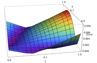
Figure 1: The absolute error graph for $N=2$ (Problem 1) by OCPs.

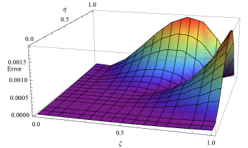
Figure 2: The absolute error graph for $N=3$ (Problem 1) by OCPs.

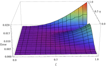
Figure 3: The absolute error graph for $N=4$ (Problem 1) by OCPs.

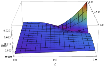
Figure 4: The absolute error graph for $N=5$ (Problem 1) by OCPs.

Problem 2. Consider the following 2-D SIVFIE :

$$f(\zeta,\eta) =g(\zeta,\eta)+\int_{0}^{1}\int_{0}^{1}(\zeta s)\sin(t+\eta)f(s,t)dtds+\int_{0}^{\zeta}\int_{0}^{\eta}(\zeta s)\sin(t+\eta)f(s,t)dtds$$

$$+\int_{0}^{\zeta}\int_{0}^{\eta}(s+t)\cos(\zeta\eta)dB(t)dB(s),$$ (6.2)

where

$$g(\zeta,\eta) =\zeta\eta+\dfrac{1}{3}(\cos(\eta+1)+\sin(\eta)-\sin(1+\eta))+\dfrac{1}{3}\zeta^{4}(\eta\cos(2\eta)+\sin(\eta)-\sin(2\eta)$$

$$-\cos(\zeta\eta)\left(\zeta^{2}B(\zeta)-2\int_{0}^{\zeta}eB(e)de\right)\left(\eta B(\eta)-\int_{0}^{\eta}B(w)dw\right)$$

$$-\cos(\zeta\eta)\left(\eta^{2}B(\eta)-2\int_{0}^{\eta}wB(w)dw\right)\left(\zeta B(\zeta)-\int_{0}^{\zeta}B(e)de\right),$$

and the exact solution of eq. (6.2) is $f(\zeta,\eta)=\zeta\eta$.

Tables 7 and 8 compare the numerical solutions to the aforementioned problem for $N=2$ and $N=3$, respectively by applying two numerical methods based on OCPs and SLPs. Table 9 represents mean, standard deviation (SD), and 95 % mean confidence interval for absolute error in $n$ trials. Table 10 shows the CPU time required by the suggested approach for various values of $N$.

Table 7: Comparison between OCPs and SLPs method for $N=2$ (Problem 2)

$(\zeta,\eta)$	Absolute error
	OCPs	SLPs
(0.05,0.05)	7.59051E-3	1.06114E-2
(0.15,0.15)	4.41259E-3	7.60286E-3
(0.25,0.25)	1.78671E-3	1.88599E-2
(0.35,0.35)	7.21046E-3	2.08891E-2
(0.45,0.45)	9.5739E-3	1.45636E-2
(0.55,0.55)	8.10448E-3	3.89986E-3
(0.65,0.65)	3.54186E-3	3.94187E-3
(0.75,0.75)	1.86214E-3	1.34215E-3
(0.85,0.85)	4.34348E-3	3.31992E-2
(0.95,0.95)	1.37409E-3	1.0822E-1

Table 8: Comparison between OCPs and SLPs method for $N=3$ (Problem 2)

$(\zeta,\eta)$	Absolute error
	OCPs	SLPs
(0.05,0.05)	6.90652E-4	2.82031E-2
(0.15,0.15)	5.00903E-3	1.22643E-2
(0.25,0.25)	6.0869E-3	1.4912E-3
(0.35,0.35)	1.10984E-3	8.77371E-3
(0.45,0.45)	1.13361E-2	1.41929E-2
(0.55,0.55)	1.48579E-2	1.35492E-2
(0.65,0.65)	3.39033E-3	1.16762E-2
(0.75,0.75)	2.2437E-2	1.32026E-2
(0.85,0.85)	4.4085E-2	7.1115E-3
(0.95,0.95)	1.4583E-2	5.78862E-2

Table 9: Mean, SD, and mean confidence interval for the absolute error in Problem 2 with $n$ trials.

$n$	$N$	Mean	SD	95% confidence interval
				Lower bound	upper bound
10	2	4.80034E-2	1.44572E-2	3.7662E-2	5.83447E-2
10	3	8.39264E-2	2.39402E-2	6.68018E-2	1.01051E-1
10	4	9.0783E-2	3.15089E-2	6.82444E-2	1.13322E-1
20	4	9.22906E-2	3.96975E-2	7.37118E-2	1.10869E-1

Table 10: CPU time (sec) for problem 2.

$N$	OCPs method	SLPs method
2	7.28	36.829
3	30.468	156.814

7 Conclusion

In this study, a new two-dimensional operational matrix method based on Chelyshkov polynomials and related operational matrices is proposed for solving 2-D SIVFIE. In this research, a novel stochastic operational matrix has been generated for the first time ever using Chelyshkov polynomials. As it is difficult to solve the Itô integral, so operational matrix for stochastic integration is beneficial to reduce 2-D SIVFIE into a system of algebraic equations, which can be further solved using the collocation approach to get the final approximate solutions. The error and convergence analysis of the newly proposed numerical technique have been rigorously established in this study. To demonstrate the efficacy and applicability of the suggested numerical approach, two illustrative examples have been solved numerically using the proposed technique. The outcomes of the numerical experiment show that there is a good agreement between the results obtained by the shifted legendre polynomials (SLPs) based numerical method and the suggested numerical method based on orthonormal Chelyshkov polynomials (OCPs). However, it is clear from the results of the numerical experiment that the suggested numerical approach is extremely effective, reliable, and accurate.
In future, we have a plan to work on 2-D nonlinear SIVFIE.

Declarations

Ethical Approval

Not applicable.

Data Availability

This article includes all the data that were generated or analysed during this research.

Competing interests

The authors assert that there are no competing interests.

Funding

NBHM, Mumbai, under Department of Atomic Energy.

Author’s contribution

All the authors have contributed equally.

References

- [1] Karimi S. and Jozi M., 2015, “A new iterative method for solving linear Fredholm integral equations using the least squares method”, Applied Mathematics and Computation, 250, pp. 744-758.
- [2] Gokme, E., Yuksel G. and Sezer M., 2017, “A numerical approach for solving Volterra type functional integral equations with variable bounds and mixed delays”, Journal of Computational and Applied Mathematics, 311, pp. 354-363.
- [3] Martire, A.L., 2022, “ Volterra integral equations: An approach based on Lipschitz-continuity”, Applied Mathematics and Computation, 435, p.127496.
- [4] Darania, P. and Ebadian, A., 2007, “ A method for the numerical solution of the integro-differential equations”, Applied Mathematics and Computation, 188(1), pp. 657-668.
- [5] Behera S., Saha Ray S., 2020, “An operational matrix based scheme for numerical solutions of nonlinear weakly singular partial integro-differential equations”, Applied Mathematics and Computation, 367, 18 pages.
- [6] Mirzaee F., Hadadiyan E., 2016, “Numerical solution of Volterra–Fredholm integral equations via modification of hat functions”, Applied Mathematics and Computation, 280, pp. 110-123.
- [7] Rahimkhani P., Ordokhani Y. and Lima P.M., 2019, “ An improved composite collocation method for distributed-order fractional differential equations based on fractional Chelyshkov wavelets”, Applied Numerical Mathematics, 145, pp.1-27.
- [8] Babaei A., Jafari H., and Banihashemi S., 2020, “A collocation approach for solving time-fractional stochastic heat equation driven by an additive noise”, Symmetry, 12(6), p.904.
- [9] Khodabin M., Maleknejad K., Rostami M. and Nouri M., 2012, “Interpolation solution in generalized stochastic exponential population growth model”, Applied Mathematical Modelling, 36(3), pp. 1023-1033.
- [10] Freund J. A. , Thorsten P., 2000, Stochastic Processes in Physics, Chemistry, and Biology, Springer-Verlag, Berlin.
- [11] Rahimkhani P. and Ordokhani Y., 2022, “ Chelyshkov least squares support vector regression for nonlinear stochastic differential equations by variable fractional Brownian motion”, Chaos, Solitons & Fractals, 163, p.112570.
- [12] Rahimkhani P. and Ordokhani Y., 2023, “ Fractional-order Bernstein wavelets for solving stochastic fractional integro-differential equations”, International Journal of Nonlinear Analysis and Applications.
- [13] Khodabin M., Maleknejad K., Rostam, M. and Nouri M., 2011,“ Numerical solution of stochastic differential equations by second order Runge–Kutta methods”, Mathematical and computer Modelling, 53(9-10), pp.1910-1920.
- [14] Mirzaee F., Samadyar N., and Hoseini S.F., 2017,“ A new scheme for solving nonlinear Stratonovich Volterra integral equations via Bernoulli’s approximation”, Applicable Analysis, 96(13), pp.2163-2179.
- [15] Mirzaee F., and Alipour S., 2020, “Cubic B-spline approximation for linear stochastic integro-differential equation of fractional order”, Journal of Computational and Applied Mathematics, 366, p.112440.
- [16] Fallahpour M., Khodabin M. and Maleknejad K., 2016,“ Approximation solution of two-dimensional linear stochastic Volterra-Fredholm integral equation via two-dimensional Block-pulse functions”,International Journal of Industrial Mathematics, 8(4), pp.423-430.
- [17] Mirzaee F., Solhi E., and Samadyar N., 2021,“ Moving least squares and spectral collocation method to approximate the solution of stochastic Volterra–Fredholm integral equations”, Applied Numerical Mathematics, 161, pp.275-285.
- [18] Mirzaee F., and Samadyar N., 2019, “On the numerical solution of fractional stochastic integro-differential equations via meshless discrete collocation method based on radial basis functions”, Engineering Analysis with Boundary Elements, 100, pp.246-255.
- [19] Sahu P. K., Saha Ray S., 2015, “A new numerical approach for the solution of nonlinear Fredholm integral equations system of second kind by using Bernstein collocation method”, Math. Meth. Appl. Sci., 38, pp. 274-280.
- [20] Ganji R.M., Jafari H., and Nemati S., 2020, “A new approach for solving integro-differential equations of variable order”, Journal of Computational and Applied Mathematics, 379, 2020, 112946.
- [21] Saha Ray S., Singh P., 2021, “Numerical solution of stochastic Itô-Volterra integral equation by using Shifted Jacobi operational matrix method”, Applied Mathematics and Computation, 410, p.126440.
- [22] Assari P., Dehghan M., 2019, “A meshless local discrete Galerkin (MLDG) scheme for numerically solving two‐dimensional nonlinear Volterra integral equations”, Journal of Computational and Applied Mathematics, 350, pp. 249‐265.
- [23] Talaei Y., and Asgari M.J.N.C., 2018,“ An operational matrix based on Chelyshkov polynomials for solving multi-order fractional differential equations”, Neural Computing and Applications, 30(5), pp.1369-1376.
- [24] Hosseininia M., Heydari M.H., and Maalek Ghaini F.M., 2021,“ A numerical method for variable-order fractional version of the coupled 2D Burgers equations by the 2D Chelyshkov polynomials” Mathematical Methods in the Applied Sciences, 44(8), pp.6482-6499.
- [25] Øksendal B., 2003, “Stochastic differential equations”, In Stochastic differential equations Springer, Berlin, Heidelberg, pp. 65-84.
- [26] Fallahpour M., Khodabin M. and Maleknejad K., 2017, “ Theoretical error analysis and validation in numerical solution of two-dimensional linear stochastic Volterra-Fredholm integral equation by applying the block-pulse functions”,Cogent Mathematics, 4(1), p.1296750.