The Theoretical Limits of Biometry

Abstract

Biometry has proved its capability in terms of recognition accuracy. Now, it is widely used for automated border control with the biometric passport, to unlock a smartphone or a computer with a fingerprint or a face recognition algorithm. While identity verification is widely democratized, pure identification with no additional clues is still a work in progress. The identification difficulty depends on the population size, as the larger the group is, the larger the confusion risk. For collision prevention, biometric traits must be sufficiently distinguishable to scale to considerable groups, and algorithms should be able to capture their differences accurately.

Most biometric works are purely experimental, and it is impossible to extrapolate the results to a smaller or a larger group. In this work, we propose a theoretical analysis of the distinguishability problem, which governs the error rates of biometric systems. We demonstrate simple relationships between the population size and the number of independent bits necessary to prevent collision in the presence of noise. This work provides the lowest lower bound for memory requirements. The results are very encouraging, as the biometry of the whole Earth population can fit in a regular disk, leaving some space for noise and redundancy.

Keywords Biometry  $\cdot$ Identification  $\cdot$ Template size  $\cdot$ Biometric information  $\cdot$ Noise  $\cdot$ Error  $\cdot$ Modeling

1 Introduction

There are three ways to prove your identity or your ownership:

• Knowledge: a password or a PIN,

• Belongings: a key (a physical object or a binary file), a smartphone, a (smart) card, a passport,

• Being: a physiological or behavioral trait: this is biometry.

Knowledge and belongings are strong evidence: they match or do not; there is no uncertainty. One single character difference within a password prevents a user from logging in. A password can be shared, but an object cannot be duplicated easily, unless it is digital. The main problem with passwords is remembering several passwords with sufficient security. Human brains need help remembering more than three passwords. On the other hand, a password makes generating strong, diverse password easy but requires the file to be stored somewhere. Computer failures make password inaccessible.

Biometry is an alternative to these two options: it is always with us and difficult to copy. On the one hand, it prevents from sharing access to a sibling. On the other hand, it prevents unauthorized users from claiming to be you, as making a counterfeit is very difficult.

The main problem of biometry is the accuracy of the systems. First, selected traits must be permanent. Hopefully, the iris, fingerprints, and veins are long-term attributes, unless surgery is done. Next, we need accurate sensors and good algorithms. During the last 20 years, there has been major progress in capturing devices where their capturing quality has improved. These improvements have a direct impact by reducing noise, improving results’ quality. With a growing interest in biometrics, researchers have improved the accuracy of their algorithms, and were able to study their results over large populations. These improvements have led to better performance and more reliable results. However, there is still room for improvement, as error rates are not yet absolute zeros.

In Biometry, there are two ways to perform authentication:

• Verification, or $1:1$ authentication: the user claims "I am X", and the system compares the freshly captured probe to the stored reference of X,

• Identification, or $1:n$ authentication: the user only provides his biometric attribute. The system compares this probe to all stored references and returns the identity associated with the best matching reference.

Today, most research focuses on verification, a kind of "two-factor authentication": you need to claim your ID thanks to a smart card, an ID card, or by spelling it, and to show one or several biometric attributes. Therefore, you need to be and have the knowledge or a physical token to be authenticated.

In the ideal world, we no longer need to carry our ID cards or passports. Our biometric attributes will be sufficient. This is the identification target, recognizing you among a large list of candidates. This task is much more difficult as there is no additional information about the user. The traits and recognition algorithm should enforce sufficient distinguishability to prevent misrecognition.

The goal of this article is to study the limits of biometrics. We provide simple relationships between the population size and the number of bits necessary to prevent collisions. We additionally consider account the impact of noise, which greatly impacts recognition performances.

The article is structured in the following way:

• In the following part, we present some previous works that have been done to evaluate the distinguishability of a biometric system.

• Next, we propose a theoretical analysis of the number of bits necessary to prevent collision between templates.

• After that, we study the impact of noise on the recognition performances.

• Then, we link our findings to traditional error rates by introducing a decision threshold.

• We present the numerical results in a dedicated part.

• Finally, we conclude this article and suggest research directions.

2 Related Works

Biometry is an experimental science, where most papers describe how data are collected and processed and how to measure the distance between two templates. One biometric system is compared to another one mainly by looking at the error rates: the False Negative Rate and False Acceptance Rate (FNR/FAR) for verification, and the False Negative Identification Rate and the False Positive Identification Rate (FNIR /FPIR) for identification. The negative and positive rate are functions of a decision threshold, where if the acceptance threshold is reduced, i.e., the difficulty is raised, then the negative rate increases while the positive rate decreases. It is common to share the equal error rate (EER), to compare two systems from a fair perspective, which is the value for which $EER=FNR=FAR$, or equivalently $EER=FNIR=FPIR$ for identification.

These error rates are computed on a database with a specific size, and the population size varies a lot from one study to another. The problem is that the error rate depends on the database size. If the database is small, the average distance between templates is large. However, the distance between templates is reduced when the database size increases, and the risk of making errors increases. Therefore, the EER allows comparing two biometric systems only if the two databases are approximately the same size.

To downplay the problem of generalization, researchers started to study biometry from a more theoretical perspective. The first works have been done on iris codes [1], [2], recognized as one of the most reliable biometrics. Iris codes are binary vectors of fixed length, which are easy to study and manipulate. The authors measured the Hamming distance between iris codes from different eyes and modeled the distribution using binomial law. Using the observed mean and variance, they estimated the number of degrees of freedom to $244$ in the first work and $249$ in the second.

Degrees of freedom are synonymous with diversity, i.e., the maximal number of different possible patterns, which in the case of iris is about $2^{249}\approx 5.63\times 10^{14}$ However, diversity does not mean “maximal number of users.” We need to take into account the distinguishability. Two users may have distinct iris codes. However, this does not imply that iris codes are distinguishable. Indeed, when performing several captures, some differences appear due to noise (pupil dilatation, slight rotation of the head, analog to digital conversion, light conditions, …): for one user, we may observe several close iris codes. Therefore, there must be a sufficient distance between the two users to consider intra-variations. In these former works, the authors studied the intra-distances between iris codes from the same person and analyzed the impact of the decision threshold on the FNR and FAR.

The works done on the iris were adapted to finger veins  [3]. There are different ways to process veins. One is to extract the location of vein lines and crossing points as it is classically done for fingerprints. Another way is to stay at the image level. In the work of  [3], pixels were classified into three categories: vein, background or unknown. Two images were compared pixel by pixel, where a mismatch rate was computed. This rate was defined as the ratio of non-overlapping vein pixels over the total vein pixels. Due to the slight difference between the mismatch rate and Hamming distance, the intra and inter distribution were modeled using a beta-binomial distribution. They obtained results similar to iris codes, demonstrating the suitability of finger vein patterns for a large population.

These previous works cannot be transposed to other biometrics easily, as each biometric has its data structure. We need to define for each case how distances between templates are measured and how distance distributions are modeled. Computing the distances between templates is often a trivial question, as the biometric system’s matcher is responsible for this task. However, the intra and inter-distribution modling must be done case by case.

Another example where the modeling differs from the two previous examples is fingerprints. A fingerprint is often represented as the list of minutiae with their location $(x,y)$ and angle $\theta$  [4]. In that case, the Hamming distance makes no sense. Instead, the authors measured the probability of random correspondence (PRC), which is the probability that two templates share a sufficiently large number of minutiae. This work has an angle model, and a model for minutiae location, and how the PRC is computed depends greatly on this modeling. Results from one model to another vary greatly and depend on the assumptions made. Fingerprints is one of the oldest biometry, and many works have been done on this topic. Nevertheless, there has yet to be a consensus on the PRC where, from one work to another, the PRC ranges between $10^{-80}$ and to $10^{-11}$  [5]. These values are the two extremes, and most works suggest a probability between $10^{-60}$ and $10^{-20}$. However, over time and research progress, the value still changes from one study to another.

These previous works illustrate the heterogeneity of biometry and the way error rates are computed.

A few works are trying to suggest a general methodology to compute the biometric information (BI), as if biometrics were a channel to transmit information  [6]. The BI is defined as “the decrease in uncertainty about the identity of a person due to a set of biometric measurements.” Mathematically, it is defined as the Kullback-Leibler divergence $K(\mathbf{p}\|\mathbf{q})$ where $\mathbf{p}$ is the intra-distribution and $\mathbf{q}$ the inter-distribution. The larger the $KL$ is, the more distinct those distributions and the easier it is to recognize any individual. The KL divergence is also called the relative entropy as $K(\mathbf{p}\|\mathbf{q})=H^{*}(\mathbf{p},\mathbf{q})-H(\mathbf{p})$, where $H$ is the Shannon entropy and $H^{*}$ is the cross entropy. In other words, the KL divergence represents the extra cost of encoding $\mathbf{p}$ using the codebook of $\mathbf{q}$.

The BI aggregates the intra and inter-distribution information into a single number, where there is no need to define a threshold. This is another way to look at the problem of distinguishability. This approach has two problems: the first is the modeling of $\mathbf{p}$ and $\mathbf{q}$, which needs to be solved case by case. The second, shared with other works like  [1] and  [3] is that getting an accurate intra-distribution $\mathbf{p}$ is difficult. Indeed, when we have a database with $n$ users and $k$ images per user, we have $\frac{n\times(n-1)}{2}k^{2}$ pairs that can be used to compute $\mathbf{q}$. However, for $\mathbf{p}$, we only have $n\times\binom{k}{2}$ pairs of images. In other words, we have around $n$ times less pairs to compute $\mathbf{p}$ than for $\mathbf{q}$.

In the former work of  [6], BI is computed using features. Modeling templates in a high dimensional space is difficult, and sometimes, their dimensionality exceeds the number of samples, making the direct use of PCA impossible. To remove the problem of high dimensionality,  [7] and  [8] suggest looking at score or distance distributions to facilitate the computation. They also suggest using a nearest neighbors’ estimator to improve the computation of $\mathbf{p}$ using a few samples. These notions of biometric information can easily be generalized to multimodal biometrics  [9]. The normalized relative entropy was derived from the BI by  [10], where the normalization aims to estimate how much the considered system can be improved.

BI, degrees of freedom, and PRC are not directly equivalent. However, they represent the limit of the biometric system considered. When looking at numerical values, there is a large gap between the results obtained from one approach to another. While  [2] claims $249$ degrees of freedom for iris,  [11] $723$ for finger veins,  [6] $46.9$ bits for face recognition, other works claim much lower values, such as $12.62$ bits for face recognition and $12.67$ for fingerprints  [9], and only 10 for iris  [7]. Due to the authors’ lack of diversity, it is unclear if these differences are due to the approach selected or the accuracy of the processing and/or the database quality.

Rather than evaluating another biometric system where our results would be correlated to our ability to create a strong and accurate biometric system, this work is purely theoretical. We propose analyzing of the minimal number of bits necessary to prevent collision and confusion as a function of the population size. Because of its simplicity, we focus on templates as arrays of random uncorrelated bits, as for iris codes. We consider noise in the matching process, as two captures are always different. The binary array model does not fit all biometric systems. The uncorrelated bits hypothesis might be far from the reality where correlations between features exist and people from the same family may have similar traits. Nonetheless, this model provides a lower bound for template size due to these ideal conditions. This gives us an estimate of the achievable maximal compression level and minimal storage requirements.

3 The Birthday Paradox

3.1 A Short Reminder

What is the probability that at least two persons in the room were born the same day?

When asking this question, most people would say this probability is very low. However, in a room of 30 people, this probability is already close to $70\%$.

In biometry, we have $N$ users enrolled in a database, each represented by a template, which is information extracted (most of the time) from a raw image. These templates are supposed to be random; sometimes, two users would get the same templates by chance. In that case it will be impossible to distinguish the two users. We want to find how to compute the template collision probability to prevent this event from happening, which is the same thing as the birthday paradox.

To compute the collision probability, the simplest way is to compute the probability of the complementary event, i.e., the probability that no one is born on the same day. Assuming there are $N$ persons and $D$ days, we have:

• User $1$ has $D$ choices for his birthday,

• User $2$ has $D-1$ choices for his birthday,

• …

• User $N$ has $D-N+1$ choices.

Therefore, there are several different ways to select birthdays are:

$$D\times(D-1)\times...\times(D-N+1)=\frac{D!}{(D-N)!}$$

Next, we need to remember that each selected date is equiprobable, with a probability of $\frac{1}{D}$. Therefore, the probability that two persons in a room were born on the same day is:

$$\begin{array}[]{ll}P(\text{At least 2 born the same day})&=1-P(\text{No one born the same day})\\ &=1-\frac{D!}{(D-N)!}\times\frac{1}{D^{N}}\end{array}$$ (1)

3.2 Computing the Collision Probability with Large Numbers.

We cannot play on the number of days in a year, but we can play on the template length, denoted $k$. Therefore, we denote $T=2^{k}$ the total number of possible patterns which replaces $D$ in the previous equation Eq. 1.

The population on Earth is currently close to $10^{10}$. The previous equation Eq. 1 contains factorials. Computing factorials up to $1000!$ is fine. However, computing factorials up to $10^{10}$ (and even above) accurately is intractable without approximation. Therefore, in this section, we provide an upper and lower bound to Eq. 1 to capture the main behavior.

With a product of large numbers, the most intuitive thing to do is to move to the log scale: We obtain $\log\left(\frac{T!}{(T-N)!}\right)=\sum_{i=T-N+1}^{T}\log(i)$ which cannot be more simplified. We can bound it by the left and by the right with integrals:

$$\int_{T-N}^{T}\log(x)dx\leq\sum_{i=T-N+1}^{T}\log(i)\leq\int_{T-N+1}^{T+1}\log(x)dx$$ (2)

Analytical solution of the $\log$ integral is obtained by integrating by part:

$$\int_{a}^{b}\log(x)dx=\left[x\log x\right]_{a}^{b}-\int_{a}^{b}\frac{x}{x}dx=\left[x(\log x-1)\right]_{a}^{b}$$ (3)

3.2.1 Lower Bound $f_{low}(T,N)$

To get the lowest bound of Eq. 2, we set $a=T-N$ and $b=T$ in Eq. 3, leading to:

$$\begin{array}[]{ll}f_{low}(T,N)&=T(\log T-1)-(T-N)\left(\log(T-N)-1\right)\\ &=T\log T-(T-N)\log(T-N)-N\end{array}$$

We can subtract the $\frac{1}{T^{N}}$ part to get the $\log$ of the probability:

$$\begin{array}[]{ll}\log\left(P_{low}(\text{No collision})\right)&=f_{low}(T,N)-N\log(T)\\ &=(T-N)\log\frac{T}{T-N}-N\\ \end{array}$$

We can get the two partial derivatives:

$$\begin{array}[]{ll}\frac{\partial P_{low}}{\partial N}&=-\log\frac{T}{T-N}+\frac{T-N}{T-N}-1\\ &=-\log\frac{T}{T-N}\\ &=\log\frac{T-N}{T}<0\end{array}$$

$$\begin{array}[]{ll}\frac{\partial P_{low}}{\partial T}&=\log\frac{T}{T-N}+(T-N)\left[\frac{1}{T}-\frac{1}{T-N}\right]\\ &=\log\frac{T}{T-N}+\frac{T-N}{T}-1\\ &=\log\frac{T}{T-N}+1-\frac{N}{T}-1\\ &=\log\frac{(T-N)+N}{T-N}-\frac{N}{T}\\ &\approx\frac{N}{T-N}-\frac{N}{T}=\frac{N^{2}}{T(T-N)}>0\end{array}$$

Assuming that $T$ is fixed, if $N$ increases, then the collision probability increases (the no-collision probability decreases), and inversely, when $N$ is fixed and $T$ increases, the collision probability decreases, which follows the natural intuition.

3.2.2 Upper Bound $f_{up}(T,N)$

We can re-do the same exercise with the upper bound, to ensure the behavior is the same on both sides. Here, we update Eq. 3 by setting $a=T-N+1$ and $b=T+1$:

$$\begin{array}[]{ll}f_{up}(T,N)&=(T+1)(\log(T+1)-1)-(T-N+1)\left(\log(T-N+1)-1\right)\\ &=(T+1)\log(T+1)-(T-N+1)\log(T-N+1)-N\end{array}$$

Last, we subtract the $\frac{1}{T^{N}}$ part:

$$\begin{array}[]{ll}\log\left(P_{up}(\text{No collision})\right)&=f_{up}(T,N)-N\log(T)\\ &=(T+1)\log(T+1)-(T-N+1)\log(T-N+1)-N-N\log T\\ &=(T+1)\log\frac{T+1}{T-N+1}-N\log\frac{T}{T-N+1}-N\end{array}$$

Deriving the two equations leads to very similar results.

3.2.3 Error Analysis

To see how well this approximation does, we can measure the difference between $f_{up}$ and $f_{low}$, as the $\log(\frac{1}{T^{N}})$ would not impact the result:

$$\begin{array}[]{ll}\Delta&=f_{up}-f_{down}\\ &=\log(T+1)+T\log\frac{T+1}{T}-\log(T-N+1)-(T-N)\log\frac{T-N+1}{T-N}\\ &=\log\frac{T+1}{T-N+1}+T\log\frac{T+1}{T}-(T-N)\log\frac{T-N+1}{T-N}\end{array}$$

To simplify this expression, we will approximate the $\log$, re-write them as $\log(1+x)$ where $x$ is small relatively close to $0$. In that case, the $\log$ terms can be approximated using:

$$\lim_{x\rightarrow 0}\log(1+x)=x-\frac{x^{2}}{2}+\frac{x^{3}}{3}-....$$

The first order is sufficient in our case. Therefore the terms are approximated as follows:

$$\begin{array}[]{lll}\log\frac{T+1}{T-N+1}&=\log\left(1+\frac{N}{T-N+1}\right)&\approx\frac{N}{T-N+1}\\ \log\frac{T+1}{T}&=\log\left(1+\frac{1}{T}\right)&\approx\frac{1}{T}\\ \log\frac{T-N+1}{T-N}&=\log\left(1+\frac{1}{T-N}\right)&\approx\frac{1}{T-N}\end{array}$$

For the term $\frac{N}{T-N+1}$, the approximation is valid only if $T\gg N$, which can be verified experimentally (for $T=365$ and $N=30$, $T$ is already ten times larger than $N$).

Replacing the logs in the previous equation, we obtain:

$$\begin{array}[]{ll}\Delta&=\frac{N}{T-N+1}+T\frac{1}{T}-(T-N)\frac{1}{T-N}\\ &=\frac{N}{T-N+1}+1-1\\ &=\frac{N}{T-N+1}\end{array}$$

So, the greater $T$ is relative to $N$, the lower the difference between the upper and the lower bound. As a reminder, $\Delta$ is the difference between the log probabilities. Therefore, $\exp(\Delta)$ is the ratio between the upper and lower bound, which we expect to be close to $1$. If $T=xN-1$ where $x$ is a positive value, then $\Delta=\frac{1}{x}$. If we suppose that $x=100$, then $\exp(\Delta)=1.01$. In other words, there is a difference of $1\%$ between the upper and the lower bound, which is an acceptable error level.

Because of this small approximation rate, we will work on the lower bound in the rest of this section, as its expression is much simpler to manipulate.

3.3 Preventing Collision

Intuitively, the number of patterns $T$ needs to be adapted to the number of users $N$. To simplify the problem and the analysis, we express $T$ as a function of $N$ by setting $T=xN$ where $x\in\mathbb{R}^{+*}$. After replacing $T$ by $xN$, the lower bound becomes:

$$\begin{array}[]{ll}\log\left(P_{low}(\text{No collision})\right)(N,x)&=(xN-N)\log\frac{xN}{xN-N}-N\\ &=N\left[(x-1)\log\frac{x}{x-1}-1\right]\end{array}$$

This is the simplest form to compute the collision probability as a function of $N$.

3.3.1 Error Rate.

The collision probability can never be exactly equal to zero. Instead, we can guarantee that this probability is less than a limit value $\alpha$ which is the tolerated error rate.

$$\alpha>P(\text{Collision})$$

$$1-\alpha\leq P(\text{No Collision})$$

With a fixed $N$ and $\alpha$, we can search for the smallest $x$ which satisfies the condition:

$$\log(1-\alpha)<N\left[(x-1)\log\frac{x}{x-1}-1\right]$$

We can re-write the $\log$ expression as $\log\frac{x}{x-1}=\log\left(1+\frac{1}{x-1}\right)$, and use the log approximation when $\frac{1}{x-1}\rightarrow 0$. The expression is simplified for large $x$ as:

$$\begin{array}[]{ll}\log(1-\alpha)&<N\left[(x-1)(\frac{1}{x-1}-\frac{1}{2(x-1)^{2}})-1\right]\\ &<-\frac{N}{2(x-1)}\end{array}$$

Re-arranging the terms to isolate $x$, we get:

$$x>-\frac{N}{2\log(1-\alpha)}+1$$ (4)

3.3.2 Analysis

Usually, the FNIR or FPIR of $5\%$ can be tolerated for non-critical applications, but is unsuitable for high stake applications such as financial services. Nevertheless, $\alpha$ is neither the FNIR nor the FPIR. FPIR and FNIR are error rates per transaction. In other words, the larger the number of users, the larger the number of errors. Here, $\alpha$ is the probability of having at least two identical templates on the enrolled population. Therefore, the probability per user would be approximately $\frac{\alpha}{N}\approx\frac{1-P(\text{No collision})}{N}$. Therefore, even if $\alpha$ is not very low (a few percent), the collision rate per transaction $\frac{\alpha}{N}$ would be relatively small.

If we look at Eq. 4, the term $-\frac{1}{2\log(1-\alpha)}$ is greater than $1$ for $\alpha<40\%$. When $\alpha=40\%$, it means that in the good case ($60\%$ chance), there is no error at all; in the worst case, there are one or two (or a little bit more) collisions between templates. For a population of one million, the individual error rate is about $10^{-6}$ which is acceptable. Accepting $\alpha=40\%$, this gives us a simple estimate for the minimal requirements for $x$:

$$x_{\alpha=0.4}=-\frac{N}{2\log(1-0.4)}+1\approx N+1>N$$

In other words, if $\alpha<\alpha_{0.4}$, then $T>T_{\alpha=0.4}=x_{0.4}N>N^{2}$. In terms of bits, for a population of $N=2^{k}$ users, we need at least $2k$ bits as $N^{2}=\left(2^{k}\right)^{2}=2^{2k}$.

3.3.3 Anti-Collision

How many additional bits are needed to reduce even more the collision probability ? We can re-write the previous equation Eq. 4 to get the number of bits as a function of the tolerance level, using the fact that for small $\alpha$, $\log(1-\alpha)\approx-\alpha$:

$$x>\frac{N}{2\alpha}+1$$

Therefore, $T_{\alpha}>\frac{N^{2}}{2\alpha}$. This represents in terms of bits:

$$\log_{2}(T_{\alpha})=\log_{2}(2^{k_{\alpha}})=k_{\alpha}>2\log_{2}(N)-1-\log_{2}(\alpha)$$ (5)

In this relationship, we see that whatever the population size, the desired accuracy is independent of the considered population. As a numerical application with $\alpha=10^{-4}$, which is a reasonable number to prevent any collision from occurring, we need $13$ extra bits to provide such a security margin. If we compute the disk space necessary for a population $N=10^{10}$ for $\alpha=0.4$ and $\alpha=10^{-4}$, we need:

• $k_{0.4}=66$ bits, leading to a total space of $76.8$ Gigabytes,

• $k_{10^{-4}}=79$ bits, leading to a total space of $92.0$ Gigabytes.

The difference in disk space between $\alpha=0.4$ and $\alpha=10^{-4}$ is relatively small, as most of the cost is due to the large number of users.

3.4 Conclusion

In this first section, we explored the Birthday Paradox, and computed an approximation for large numbers. We demonstrated that the number of possible patterns should be at least $T=N^{2}$ to prevent frequent collisions between templates from occurring, which corresponds to a minimum of $2\log_{2}(N)$ bits, which has a small impact in terms of space. We also analyzed the cost of additional security, as when $T=N^{2}$, a few collisions are still possible. Adding a security margin requires only a few extra bits, where their number is independent of the population. This opens the possibilities for large-scale biometry, as the template size can be small while providing high distinguishability.

4 Matching with Noise

In the previous section, we studied the ideal case, where there is no noise and bits follow a Bernoulli distribution with parameter $1/2$ and are independent.

In biometry, these assumptions do not often hold. Especially for noise: when placing a biometric attribute over a sensor, the outcome is almost always different, because of factors such as:

• the position is never exactly the same (translation or rotation)

• the quality of the capture may vary with many parameters, like temperature, dust, light, humidity, ….

• some internal biological changes impact the attribute (disease, physical activity, injury, stress, …)

Therefore, it is almost impossible to capture twice the same sample.

In this section, we propose to study the impact of noise on recognition accuracy.

4.1 Noise Assumption

4.1.1 Probe VS Template

In biometry, we distinguish a probe from a template: a template is a processed capture stored in a database, while a probe is a freshly processed capture to compare against stored templates. When described this way, there is no difference between a template and a probe.

In practice, a single capture is often noisy, and it is better to ask the user several times to present their biometric attribute to reduce the noise level. It is possible to ask the user to do so for enrollment, as enrollment is done only once. However, as we want the identification to be seamless, only one capture is tolerated for user convenience. Therefore, we consider that a template is “free of noise” (which is not exactly true, as there is always residual noise), while a probe is always noisy.

4.1.2 Probability Distributions

We still suppose that bits follow a Bernoulli distribution of parameter $1/2$ and are uncorrelated. We assume that probes are affected by noise with level $2p$. We put a factor $2$ to consider bits that are affected by noise but unchanged. On average, $p$ will be flipped (i.e., $0\rightarrow 1$ and $1\rightarrow 0$), while a proportion $p$ will stay at its initial value ($0\rightarrow 0$, $1\rightarrow 1$). For the following, it is easier to think in terms of “flip” probability $p$, ranging from $0$ to $0.5$, as the interval $[0.5,1]$ is symmetric. In the displayed graphics, we will print $2p$, to present results over an interval ranging from $0$ to $1$.

The intra-distribution of Hamming distances follows a Binomial distribution of parameter $(k,p)$, where $k$ is the length of the probe (and template). In contrast, the inter-distribution follows a binomial distribution of parameter $(k,1/2)$, as random noise effects compensate.

4.2 Recognition Probability

To measure the overall probability of making an identification error, we first need to look at the probability of recognizing one specific user. If there are $n$ templates in the database, we need to compute the Hamming distance between the probe and the $n$ templates, and select the identity of the template with the lowest distance. For simplicity, we suppose there is only one template with the lowest distance, i.e., no ex-aequo for the winning place.

We denote the distance between the probe and the corresponding template $d$. It ranges between $0$ (no error) and $k$ (only errors), but the correct template would never be recognized in the latter case. To be recognized correctly, the intra-distance $d$ can be greater than $0$, as long as the distance between the probe and the other non-matching templates is larger than $d$.

The probability that the distance between the probe and the corresponding template is equal to $d$ is:

$$P(D=d;p)=\binom{k}{d}p^{d}(1-p)^{k-d}$$

The probability that the distance between the probe and another non-matching template is greater than $d$ is:

$$P(D\geq d+1;\frac{1}{2})=\frac{1}{2^{k}}\sum_{i=d+1}^{k}\binom{k}{i+1}$$

Assembling these two previous equations, the probability that the user (denoted $u$) is correctly recognized is:

$$\begin{array}[]{ll}P(u;p,n)&=\sum_{d=0}^{k-1}\left[P(D=d;p)\times P(D\geq d+1;\frac{1}{2})^{n-1}\right]\\ &=\sum_{d=0}^{k-1}\left[\binom{k}{d}p^{d}(1-p)^{k-d}\times\left(\frac{1}{2^{k}}\sum_{i=d+1}^{k}\binom{k}{i}\right)^{n-1}\right]\end{array}$$ (6)

The power $n-1$ considers the other patterns against which the distance should not be lower or equal to $d$.

4.3 Group Recognition

In the previous paragraph, we looked at the probability of correctly identifying one user among a group. Now, we want to find the probability that all users $u_{1},u_{2},...,u_{n}$ are correctly recognized. We can express the global probability using the Bayes decomposition rule:

$$\begin{array}[]{ll}P(\text{Accept All})&=P(u_{1},u_{2},...,u_{N})\\ &=P(u_{1})P(u_{2},...,u_{N}|u_{1})\\ &=P(u_{1})P(u_{2}|u_{1})P(u_{3},...,u_{N}|u_{1},u_{2})\end{array}$$

Here, we consider that an identification outcome depends on the previous ones. If $u_{1},u_{2},...,u_{i}$ have been correctly identified so far, then $u_{i+1}$ cannot be mistaken as one of these previously identified users, as errors are symmetric. This only holds because we consider the case where there is no identification error at all. Therefore, the overall acceptance probability is:

$$\begin{array}[]{ll}P(\text{Accept all},p,N)&=\prod_{i=1}^{N}P(\text{One user recognized among }i\text{ users})\\ &=\prod_{i=1}^{N}P(u;p,i)\\ &=\prod_{i=1}^{N}\sum_{d=0}^{k-1}P(D=d;p)\times P(D\geq d+1;\frac{1}{2})^{i-1}\end{array}$$ (7)

4.3.1 Case where $p=0$

When there is no noise, we should get the same results as in the previous part. The distance between the probe and the corresponding template must be exactly $0$. Therefore, the sum in Eq. 7 can be simplified as only the first term $P(D=d;p)$ is equal to $1$ while all others are equal to $0$. Next, the inter-probability is obtained by using the complementary event $P(D\geq 1;\frac{1}{2})=1-P(D=0;\frac{1}{2})$:

$$\begin{array}[]{ll}P(\text{Accept all};p=0,N)&=\prod_{i=1}^{N}1\times P(D>0;p=\frac{1}{2})^{N-i-1}\\ &=\left(P(D>0;\frac{1}{2})\right)^{\frac{N^{2}-N}{2}}\\ &=\left(1-P(D=0;\frac{1}{2})\right)^{\frac{N^{2}-N}{2}}\\ &=\left(1-\frac{1}{2^{k}}\right)^{\frac{N^{2}-N}{2}}\end{array}$$ (8)

Now, we can re-arrange Eq. 8 to fit the organization of Eq. 4 to verify if both expressions lead to the same behavior.

First, we can replace $2^{k}$ by $T$ the number of possible templates and move to the $\log$ scale:

$$\log(P(\text{accept}))=\log(1-\alpha)=\frac{N^{2}-N}{2}\log(1-\frac{1}{T})$$

Then, the log part is approximated as $\frac{1}{T}$ is sufficiently small:

$$\log(P(\text{accept}))\approx-\frac{N^{2}-N}{2}\times\frac{1}{T}$$

And last, we can express $T$ as a function of $N$, such as $T=xN$

$$\log(P(\text{accept}))\approx-\frac{N^{2}-N}{2xN}=-\frac{N-1}{2x}$$ (9)

This expression is very close to the inequality in Eq. 4, where the $N-1$ replaces the $N$ (which has a negligible impact as $N\gg 1$), and the denominator is $2x$ in Eq. 9 instead of $2(x-1)$, where the difference does not matter either as $x$ is large.

4.4 How to Compute for $p>0$ ?

When $p>0$, the expression cannot be simplified. We can re-write Eq. 7 as:

$$P(\text{Accept all})=\prod_{i=1}^{N}\sum_{d=0}^{k-1}w_{d}\times a_{d}^{i-1}$$ (10)

where:

• $w_{d}=\binom{k}{d}p^{d}(1-p)^{k-d}$ with $\sum_{d=0}^{k-1}w_{d}=1$.

• $a_{d}=\frac{1}{2^{k}}\sum_{i=d+1}^{k}\binom{d}{i}$ with $0\leq a_{d}\leq 1$.

The terms $w_{d}$ and $a_{d}$ are the same whatever the value of $i$. The main problem is the term $a_{d}^{i-1}$ where the power makes simplification difficult.

We can provide an upper and lower bound to this value. First, we define $f(i)$ as $f(i)=\sum_{d=0}^{k-1}w_{d}a_{d}^{i-1}$, which simplify Eq. 10 into $P(\text{Accept all})=\prod_{i=1}^{N}f(i)$. Next, as $a_{d}\leq 1$, if $i<j$, then $f(i)\geq f(j)$. Therefore:

$$f(N)^{N}\leq P(\text{Accept all})\leq f(1)^{N}$$

These bounds are too coarse to be useful. Keeping this approximation idea in mind, let’s say that we cut into $z$ intervals our $N$ users, such as $[n_{0}=1,n_{1},n_{2},...,n_{z}=N|n_{i}<n_{i+1}]$. We can re-write the product into multiple sub-products:

$$P(\text{Accept all})=\prod_{i=0}^{z-1}\prod_{j=n_{i}}^{n_{i+1}}f(j)$$

Given the previous trick, we can provide a more accurate bounding:

$$\prod_{i=0}^{d-1}f(n_{i+1})^{n_{i+1}-n_{i}}\leq P(\text{Accept all})\leq\prod_{i=0}^{d-1}f(n_{i})^{n_{i+1}-n_{i}}$$ (11)

4.4.1 Numerical Tests

In the following table Table 1, we reported the exact value $v_{truth}=P(\text{Accept alll})$ and compared it to the lower bound $v_{low}$ and upper bound $v_{high}$. The approximations were done using $100$ intervals of equal size (± 1 element).

Table 1: Approximation error done with Eq. 11

$k$	$n$	$p$	$v_{low}$	$v_{truth}$	$v_{high}$	$\Delta=\frac{v_{high}-v_{low}}{2v_{truth}}$
20	$1,000$	0.001	$0.559$	$0.562$	$0.566$	0.58 %
25	$1,000$	0.001	$0.98$	$0.98$	$0.981$	0.02 %
20	$1,000$	0.01	$0.161$	$0.164$	$0.167$	1.8 %
25	$1,000$	0.01	$0.904$	$0.905$	$0.906$	0.1 %
30	$1,000$	0.01	$0.994$	$0.994$	$0.995$	0.00556 %
50	$1,000$	0.2	$0.467$	$0.47$	$0.474$	0.709 %
150	$10,000$	0.4	$0.615$	$0.618$	$0.621$	0.451 %
35	$100,000$	0.01	$0.0464$	$0.0478$	$0.0493$	3.06 %
35	$100,000$	0.001	$0.779$	$0.781$	$0.783$	0.25 %
35	$100,000$	0.0001	$0.855$	$0.857$	$0.858$	0.156 %
45	$1,000,000$	0.01	$0.369$	$0.373$	$0.377$	0.994 %

As you can see, the absolute and relative errors are relatively low. Therefore, we consider this approximation as accurate enough for our application.

In the next part, we will investigate the behavior in the open world, where one part of the population is unenrolled.

5 Open-World

In the two previous sections, we studied the case where all users are enrolled. Therefore, there cannot be false positives. In real life, there are many people unknown from the biometric system. Therefore, identification should first decide between two main cases: is the person enrolled or not? If the person is enrolled, an identity is returned.

It is common to set a decision threshold $thr$to make this initial decision: if the distance between the probe and the closest template is less or equal to $thr$, then the system considers the user enrolled.

5.1 Error Rates

5.1.1 FNIR

Because of the threshold, an enrolled user will sometimes not be recognized appropriately ($FNIR$). There are two complementary sub-cases:

1. No identity is returned ($FNIR_{n}$)

2. An identity is returned, but not the correct one ($FNIR_{i}$)

When no identity is returned, the distance between the probe and any template (the correct one and all $N-1$ incorrect others) is greater than $thr$. It is computed as:

$$FNIR_{n}=P(D>thr,p)\times P\left(D>thr,\frac{1}{2}\right)^{N-1}$$

The second case is the confusion probability, which is the probability of taking someone for someone else. This is when at least one incorrect template is closer than the correct one and this distance is lower than the threshold.

$$FNIR_{i}=\sum_{d=1}^{thr}P(D=d,p)\times\left(1-P\left(D>d,\frac{1}{2}\right)^{N-1}\right)$$

5.1.2 FPIR

In the open world setup, there are unenrolled people that the system will try to identify. We get a false positive match if the distance between the probe and at least one template is under the decision threshold:

$$FPIR=1-P\left(D>thr,\frac{1}{2}\right)^{N}$$

Compared to the two other error rates, this one is independent of the noise level.

5.2 Trade-Off Between Parameters

We have two input variables $p$ and $N$, three constraints, and we can play on two parameters $k$ and $thr$. In these paragraphs, we will describe the methodology for setting $k$ and $thr$ efficiently.

5.2.1 $FNIR_{n}$

This error rate depends on $p$, $N$, $k$ and $thr$. Therefore, it is difficult to optimize this value due to the dependencies. The $FNIR_{n}$ is made of two parts: one which concerns the distance between the probe and the correct template, and the second concerns the relationship between the probe and all other templates. Because both are probability terms, they are bounded by $1$. By setting the second term to $1$, an upper bound for this error rate is:

$$FNIR_{n}<P(D>thr,p)$$

Here, this probability is still dependent on the three different variables (as $thr$ depends on $k$). Nevertheless, this expression is much simpler to compute. If we denote $\beta$ the maximal acceptable $FNIR_{n}$, we should search for a triplet $(thr,p,k)$ that satisfy:

$$FNIR_{n}<P(D>thr,p)\leq\beta$$ (12)

The $FNIR_{n}$ is a convenience rate as nothing is at stake. If the user is not recognized the first time, they can retry again. Therefore, this rate can be relatively high compared to the two other rates, and a maximal error rate of $5\%$ can be acceptable in real-world scenarios.

5.2.2 $\mathbf{FNIR_{i}}$

The $FNIR_{i}$ is the confusion rate, i.e., the probability of taking someone for someone else. This rate depends on the four variables, making it difficult to optimize. As for the $FNIR_{n}$, we can provide an upper bound to simplify the parameter selection process. As the larger the threshold is, the greater the $FNIR_{i}$, we set $thr=k$ to remove the threshold dependency:

$$FNIR_{i}=FNIR_{i}(thr)<FNIR_{i}(thr=k)=FNIR_{i}^{\infty}$$

The $FNIR_{i}$ is the confusion rate per transaction. Therefore, the number of errors scales linearly with the number of users trying to identify. However, we may want to guarantee a fixed error rate independent of the number of users. This was the topic of the two previous sections 3 and 4 where the global error rate can be guaranteed.

In section 3, the minimal requirement for no noise is $k>2\log_{2}(N)$. For a larger noise level, the necessary $k$ needs to be computed case by case.

5.2.3 $\mathbf{FPIR}$

The last error rate to look at is the $FPIR$, which is independent of the noise level $p$. The two $FNIR$ rates provide us the lowest acceptable values for $k$ and $thr$. When $thr$ increases, the $FPIR$ increases too, while when $k$ increases, the $FPIR$ decreases. Therefore, given the minimal $k$ provided by the $FNIR_{i}$, we need to increase it until the $FPIR$ conditions are met.

$$\begin{array}[]{ll}FPIR&=1-(1-P(D\leq thr,\frac{1}{2}))^{N}\\ &\approx 1-(1-N\times P(D\leq thr,\frac{1}{2}))\\ &\approx N\times P(D\leq thr,\frac{1}{2})\end{array}$$

The $FPIR$ is an error rate per transaction. The larger the unenrolled population $N^{-}$, the greater the number of errors.

We need to pay attention to the deployment scenario. For attended biometry, i.e., where the biometry cannot be captured without the user’s consent, the number of unenrolled persons that will try to authenticate themselves is relatively low. However, for unattended biometry, where the system will try to recognize any person (like video cameras), the number of unenrolled persons will be very large, maybe larger than the enrolled population.

The target system probability could be:

$$\begin{array}[]{ll}P\left(\text{One error over }N^{-}\text{transactions}\right)&=1-(1-FPIR)^{N^{-}}\\ &\approx 1-(1-N\times P(D\leq thr,\frac{1}{2}))^{N^{-}}\\ &\approx 1-(1-NN^{-}\times P(D\leq thr,\frac{1}{2}))\\ &\approx NN^{-}\times P(D\leq thr,\frac{1}{2})\end{array}$$

As for the $FNIR_{n}$, we can approximate $P(D\leq thr,\frac{1}{2})$ using a normal law $\mathcal{N}(k/2,\sqrt{\frac{k}{4}})$. Setting $\gamma$ as the maximal error rate for $P\left(\text{One error over }N^{-}\text{transactions}\right)$, we have:

$$thr<\frac{k}{2}-f^{-1}\left(\frac{\gamma}{NN^{-}}\right)\sqrt{\frac{k}{4}}$$ (13)

where $f^{-1}(.)$ satisfies $\gamma=P\left(Y>f^{-1}(\gamma)\right)|Y\sim\mathcal{N}(0,1)$.

5.3 Search Procedure

We can summarize the search procedure for $k$ and $thr$ by Algo. 1.

Algorithm 1 Search Procedure

$\alpha,\beta,\gamma,N,N^{-},p$

$k\leftarrow g_{1}(\alpha,N,p)$ $\triangleright$ Using Eq. 10

$flag\leftarrow\text{true}$

while $flag$ do

     $thr_{0}\leftarrow g_{2}(\beta,N,p,k)$ $\triangleright$ Using Eq. 12

     $thr_{1}\leftarrow g_{3}(\gamma,N,N^{-},k)$ $\triangleright$ Using Eq. 13

     if $thr_{0}<thr_{1}$ then

         $flag\leftarrow\text{false}$

     else

         $k\leftarrow k+1$

     end if

end whilereturn $(k,thr_{0})$

5.4 Conclusion

In this section, we have provided bounds and approximations for the three error rates in the case of an open-world situation. To satisfy these three conditions, a simple search procedure can be followed.

6 Numerical Results

In this part, we present numerical evaluations by displaying corresponding curves. In the first subpart, we study the evolution of $P(\text{Accept})$ as a function of the other parameters $k$, $p$ and $N$ the population size. In the second subpart, we fix the tolerance level $\alpha$ and study the relationships between parameters to preserve this error level. This enables us to look at two parameters at a time. After that, we model the relationships between noise, population and number of bits. Given these results, we estimate the database size requirements. Last, we evaluate these requirements in the open-world case.

6.1 $P(\text{Accept})$

6.1.1 $P(Accept)=f(N,p;k)$

In this experiment, we study the overall acceptance probability as a function of the population size for a fixed number of bits ($k=40$). We study the behavior for doubling the noise level from $0.15\%$ to $40\%$.

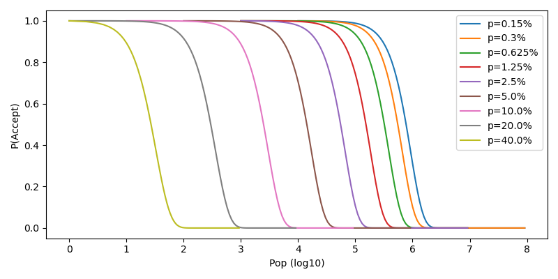
Figure 1: Encoding capacity for k=40

As expected, the larger the noise level, the smaller the population we can enroll without having high error rates. At some point, we reach a ceiling, as for $k=40$, we can enroll at best one million users without noise, as $\log_{10}(2^{40/2})\approx 6$.

6.1.2 $P(Accept)=f(N,k;p)$

Compared to the previous experiment, the noise level is fixed to $10\%$ while the number of bits is changed from $10$ to $50$ bits.

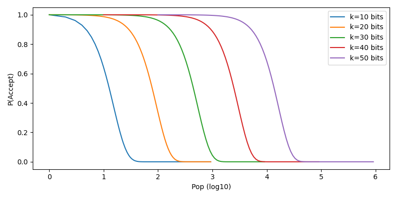
Figure 2: Encoding capacity for $p=10\%$

Even under noisy conditions, it seems that $k$ additional bits increase the capacity from $N$ to $N\times K$, where $K$ is independent of $N$. This result was proved for the no-noise case, but we could not demonstrate this due to the complexity of the noisy case. The next subsections will empirically study this relationship between bits and population.

6.1.3 $P(Accept)=f(k,p;N)$

Last, we study the resilience behavior when adding bits while increasing noise for a fixed-size population, where $N=10^{6}$. Here, the noise is increased by adding $5\%$ for each step, ranging from $5\%$ to $40\%$.

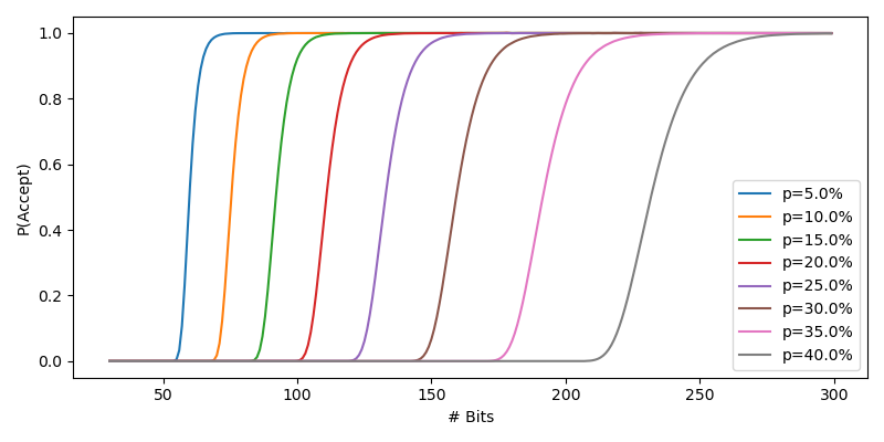
Figure 3: Numbers of bits necessary for $N=10^{6}$ for different noise levels

The relationship between the noise level and the number of bits is not linear, as we need more bits to compensate for a change from $35$ to $40\%$ of noise compared to a change from $5$ to $10\%$.

6.2 $k=f(N;\alpha)$

In many real-world applications, there is often a target accuracy to reach, or a maximal error rate. In this part, we fix simultaneously the tolerance level $\alpha=1-P(\text{Accept})$ to study two parameters.

In this experiment, we study the relationship between the number of bits and the population size and display several curves for different noise levels. We repeated the experiment for two tolerance levels, one with $\alpha=0.5$ and the other with $\alpha=0.1$.

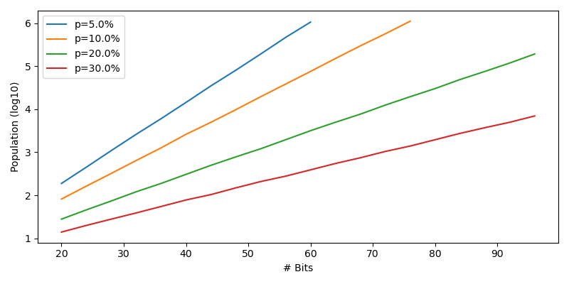
Figure 4: Tolerance level $(1-\alpha)>0.5$

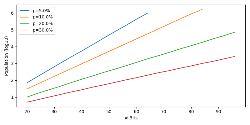
Figure 5: Tolerance level $(1-\alpha)>0.9$

We have a clear linear relationship between the population log and the number of bits, whatever the tolerance level $\alpha$ and the noise level $p$. When fitting a linear model with the form $ax+b$, the fit is very good with a $r^{2}>0.99$. The only differences between the two figures are the coefficients $a$ and $b$, which depend on $\alpha$ (and $p$).

6.3 Getting Slope Coefficients as a Function of Noise

From the previous plots, we can assume that the number of bits is linearly linked to the log population size $N$. Therefore, we can write that:

$$\log_{2}(N)=a_{p}\times k+b_{p}$$

In practice, we are more interested in the reciprocal relationship: Given a population of $N$, we want to know how many bits are necessary to prevent collision. In that case, we write the relationship as:

$$k=A_{p}\times\log_{2}(N)+B_{p}$$

where $A_{p}=\frac{1}{a_{p}}$ and $B_{p}=-\frac{b_{p}}{a_{p}}$.

We collected different coefficients $A_{p}$ and $B_{p}$ by increasing the noise level, increasing the noise by $1\%$ from $1\%$ to $50\%$, and fixed $\alpha$ to $10^{-4}$.

We limited the exploration to noise levels between $[0\%,50\%]$ for several reasons. We expect the noise in real life to be smaller than $50\%$; otherwise the capture is very inaccurate. In that case, it might be better to optimize sensor quality rather than invest in larger databases and a slower matching system. Next, even if a larger level of noise were studied, splitting the data into different intervals and fitting them separately would have been preferable, as errors on large values will mask errors on small values.

We obtained the following curves:

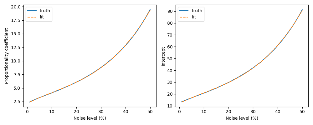
Figure 6: Coefficients curves and fit: Left: $A_{p}$, right: $B_{p}$

As you can see, the larger the noise, the larger the slope and the intercept in absolute value. We fitted a polynom of degree $3$ where the line (orange in the figure) perfectly overlaps the experimental values, where the coefficients are:

$$A(p)=1.28\times 10^{2}p^{3}-40.2p^{2}+22.4p+2.17$$

$$B(p)=5.80\times 10^{2}p^{3}-1.75p^{2}+99.8p+12.1$$

We obtained an MSE of $0.048$ for coefficients $A_{p}$ and $0.25$ for coefficients $B_{p}$. With this fit, we get $A(0)=2.17$, which is slightly greater than $2$ and an intercept of $B(0)=12.1$ which is very close to $13-1=12$ from Eq. 5 when $\alpha=10^{-4}$. These differences are acceptable for our application where we are searching for the right order of magnitude, not necessarily the exact value with no errors.

Here, the coefficients are expressed as a function of $\log_{2}(N)$, compared to $\log_{10}(N)$ in the previous choices. In the previous experiments, we studied the impact of noise and $k$ on the maximal capacity. It is much easier in that case to use the $\log_{10}(N)$, while it is much more difficult to know by heart what $2^{x}$ corresponds to. Here, we want a relationship between $k$ and $N$. In the first section, we found that $T=2^{2k}$ when $N=2^{k}$. Therefore, to compare to this first result, we expressed the coefficient $A_{p}$ in base $2$.

6.4 Biometric Database Size

Using the coefficients $A(p)$ and $B(p)$, we can estimate the size required to store templates. Here, we consider a population of ten billion, where $10^{10}\approx 2^{33.2}$. The results are listed in the following table.

Table 2: Relationship between noise, bits, and database size.

Noise level $p$ (%)	$A(p)$	$B(p)$	$k(p,N)$	DB size (GB)
0	2.17	12.1	85	98.95
5	3.21	16.7	124	144.4
10	4.14	20.9	159	185.1
15	5.06	25.1	194	225.8
20	6.07	29.7	232	270.1
25	7.26	35.2	277	322.5
30	8.74	41.9	333	387.7
35	10.6	50.4	403	469.2
40	12.9	61.1	491	571.6
45	15.8	74.4	600	698.5
50	19.4	90.7	734	854.5

As you can see, even with much noise, the whole Earth’s population can fit in a regular disk. These are encouraging results for developing identification systems, as storage size is not the limiting problem.

6.5 Open-World

So far, we have studied the confusion rate in a closed world where all the population is enrolled. Now, we can study the impact of a threshold, and see how it impacts the memory requirements.

For this experiment, we set $FNIR_{n}^{\max}=10^{-2}$, $FPIR=10^{-4}$ and $P(\text{reject all external})=10^{-4}$, as it seems reasonable values for most scenario. Here, we set $N=N^{-}=10^{10}$. The rationale of this last choice is the following: the system should be able to enroll the whole population size without any conflict ($N=10^{10}$). However, most of the population would not be enrolled on day one. Therefore, at max, we would have $10^{10}$ non-enrolled people ($N^{-}=10^{10}$).

Table 3: Threshold values for various noise level.

Noise (%)	$k_{0}$	$k$	$thr$
5	125	125	9
10	160	160	16
15	195	195	25
20	233	233	35
25	278	278	49
30	334	334	67
35	404	404	90
40	492	492	120
45	601	601	160
50	735	735	212

In Table 3, $k_{0}$ is the number of bits obtained in the closed case where there is no threshold, thanks to the coefficient $A_{p}$ and $B_{p}$. $k$ is the adjusted value in case there are the $FNIR_{n}$ and $FPIR$ constraints.

The results have been obtained by approximating the main parameters using the normal law approximations. However, due to numerical errors for low $p$, we refined the search by a local search to obtain the exact minimal parameters.

Here, surprisingly, $k_{0}=k$, i.e., no difference exists between the open-world and closed world memory requirements. This is due to the high distinguishability requirements, which makes authentication of outsiders very difficult. When the constraints for the $FPIR$ are increased, more bits are necessary for the low noise level, but there is no change when $p$ is large.

In conclusion, using a threshold to prevent unenrolled users from authenticating has a very limited impact on the memory requirements, as no extra bits are needed.

7 Conclusion

In this work, we studied the number of bits necessary to store biometric templates while avoiding collision. As data collection is subject to noise, we studied its impact in the identification case.

In the ideal case of no noise, the number of bits grows in $2\log_{2}(N)$. However, more bits are needed to compensate for uncertainty in the presence of noise. When the noise level is fixed, there is still a linear relationship between the log of the population and the number of bits necessary, which eases the estimation of the required database size. While the noise increases the need for more bits, most of the cost is associated with the number of enrolled users. When moving from $5\%$ to $50\%$ of noise, we only need to multiply by $6$ the disk space needed.

We considered the open-world setup, where one part of the population is not enrolled yet. We provided the probabilistic formulation of the $FPIR$ and $FNIR_{i}/FNIR_{n}$ as a function of the threshold. Additional bits are needed to adapt to the threshold case for a small noise level. However, the threshold has no impact for a large noise level, as the required number of bits is unchanged.

This is an encouraging step towards large-scale identification systems. Nevertheless, there are still many challenges to solve. First, all through this work, we assumed that bits are independent. Research is needed to provide efficient compression algorithms to remove redundancy from templates. Next is the matching question: how much time is required, and how can we speed up the identification process as it requires comparing all the $n$ stored templates to the probe. Last, we have the question of cancelable biometrics and secure biometric templates. As for today, while cancelable biometrics such as Biohashing  [12] enables the creation of several protected templates from a single unprotected one, the matching accuracy is often decreased. We need to study this system more in detail to provide additional security guarantees without accuracy loss in this setup.

References

- Zhou [2012] Z. Zhou. Ensemble methods: Foundations and algorithms. 2012.
- Breiman [2004] L. Breiman. Bagging predictors. Machine Learning, 24:123–140, 2004.
- Khan et al. [2020] Z. Khan, Asma Gul, A. Perperoglou, M. Miftahuddin, Osama Mahmoud, W. Adler, and B. Lausen. Ensemble of optimal trees, random forest and random projection ensemble classification. Advances in Data Analysis and Classification, 14:97–116, 2020.
- Schapire and Freund [2012] R. Schapire and Y. Freund. Boosting: Foundations and algorithms. 2012.
- Li and Ding [2008] Tao Li and C. Ding. Weighted consensus clustering. In SDM, 2008.
- Ren et al. [2013] Ya-Zhou Ren, C. Domeniconi, Guoji Zhang, and Guo-Xian Yu. Weighted-object ensemble clustering. IEEE 13th International Conference on Data Mining, pages 627–636, 2013.
- Margineantu and Dietterich [1997] D. Margineantu and Thomas G. Dietterich. Pruning adaptive boosting. In ICML, 1997.
- Fan et al. [1999] Wei Fan, S. Stolfo, and Junxin Zhang. The application of adaboost for distributed, scalable and on-line learning. In KDD ’99, 1999.
- Ormándi et al. [2013] Róbert Ormándi, I. Hegedüs, and M. Jelasity. Gossip learning with linear models on fully distributed data. Concurrency and Computation: Practice and Experience, 25, 2013.
- Abualkibash et al. [2013] Munther Abualkibash, Ahmed ElSayed, and A. Mahmood. Highly scalable, parallel and distributed adaboost algorithm using light weight threads and web services on a network of multi-core machines. ArXiv, abs/1306.1467, 2013.
- Ratasich et al. [2019] Denise Ratasich, Faiq Khalid, Florian Geissler, R. Grosu, M. Shafique, and E. Bartocci. A roadmap toward the resilient internet of things for cyber-physical systems. IEEE Access, 7:13260–13283, 2019.
- Probst and Boulesteix [2017] P. Probst and A. Boulesteix. To tune or not to tune the number of trees in random forest? J. Mach. Learn. Res., 18:181:1–181:18, 2017.
- Pes [2019] B. Pes. Ensemble feature selection for high-dimensional data: a stability analysis across multiple domains. Neural Computing and Applications, 32:5951–5973, 2019.
- Breiman [2001] Leo Breiman. Random forests. Machine Learning, 45:5–32, 2001. ISSN 0885-6125. doi:10.1023/A:1010933404324.
- Sen [2009] Jaydip Sen. A survey on wireless sensor network security. ArXiv, abs/1011.1529, 2009.
- Sheikh and Liang [2019] Muhammad Sameer Sheikh and Jun Liang. A comprehensive survey on vanet security services in traffic management system. Wirel. Commun. Mob. Comput., 2019:2423915:1–2423915:23, 2019.
- Strehl and Ghosh [2002] A. Strehl and Joydeep Ghosh. Cluster ensembles — a knowledge reuse framework for combining multiple partitions. J. Mach. Learn. Res., 3:583–617, 2002.
- Galdi et al. [2014] P. Galdi, F. Napolitano, and R. Tagliaferri. Consensus clustering in gene expression. In CIBB, 2014.
- Fred and Jain [2005] A. Fred and Anil K. Jain. Combining multiple clusterings using evidence accumulation. IEEE Transactions on Pattern Analysis and Machine Intelligence, 27:835–850, 2005.
- Monti et al. [2004] S. Monti, P. Tamayo, J. Mesirov, and T. Golub. Consensus clustering: A resampling-based method for class discovery and visualization of gene expression microarray data. Machine Learning, 52:91–118, 2004.
- Dietterich and Bakiri [1995] Thomas G. Dietterich and Ghulum Bakiri. Solving multiclass learning problems via error-correcting output codes. ArXiv, cs.AI/9501101, 1995.
- Hao et al. [2010] F. Hao, P. Ryan, and Piotr Zielinski. Anonymous voting by two-round public discussion. IET Inf. Secur., 4:62–67, 2010.
- Dua and Graff [2017] Dheeru Dua and Casey Graff. UCI machine learning repository, 2017. URL http://archive.ics.uci.edu/ml.