VREM-FL: mobility-aware computation-scheduling co-design for vehicular federated learning

Abstract

Assisted and autonomous driving are rapidly gaining momentum, and will soon become a reality. Among their key enablers, artificial intelligence and machine learning are expected to play a prominent role, also thanks to the massive amount of data that smart vehicles will collect from their onboard sensors. In this domain, federated learning is one of the most effective and promising techniques for training global machine learning models, while preserving data privacy at the vehicles and optimizing communications resource usage. In this work, we propose VREM-FL, a computation-scheduling co-design for vehicular federated learning that leverages mobility of vehicles in conjunction with estimated 5G radio environment maps. VREM-FL jointly optimizes the global model learned at the server while wisely allocating communication resources. This is achieved by orchestrating local computations at the vehicles in conjunction with the transmission of their local model updates in an adaptive and predictive fashion, by exploiting radio channel maps. The proposed algorithm can be tuned to trade model training time for radio resource usage.

Experimental results demonstrate the efficacy of utilizing radio maps. VREM-FL outperforms literature benchmarks for both a linear regression model (learning time reduced by $28\%$) and a deep neural network for a semantic image segmentation task (doubling the number of model updates within the same time window).

I Introduction

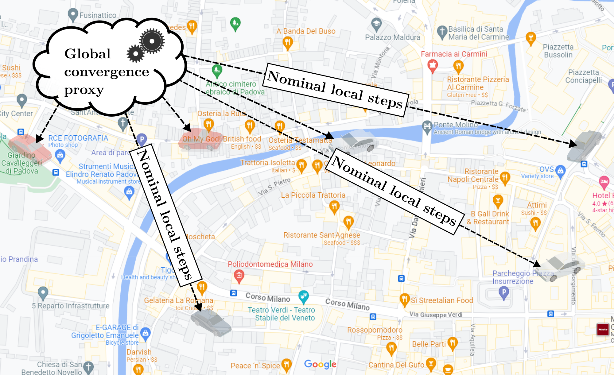
(a)

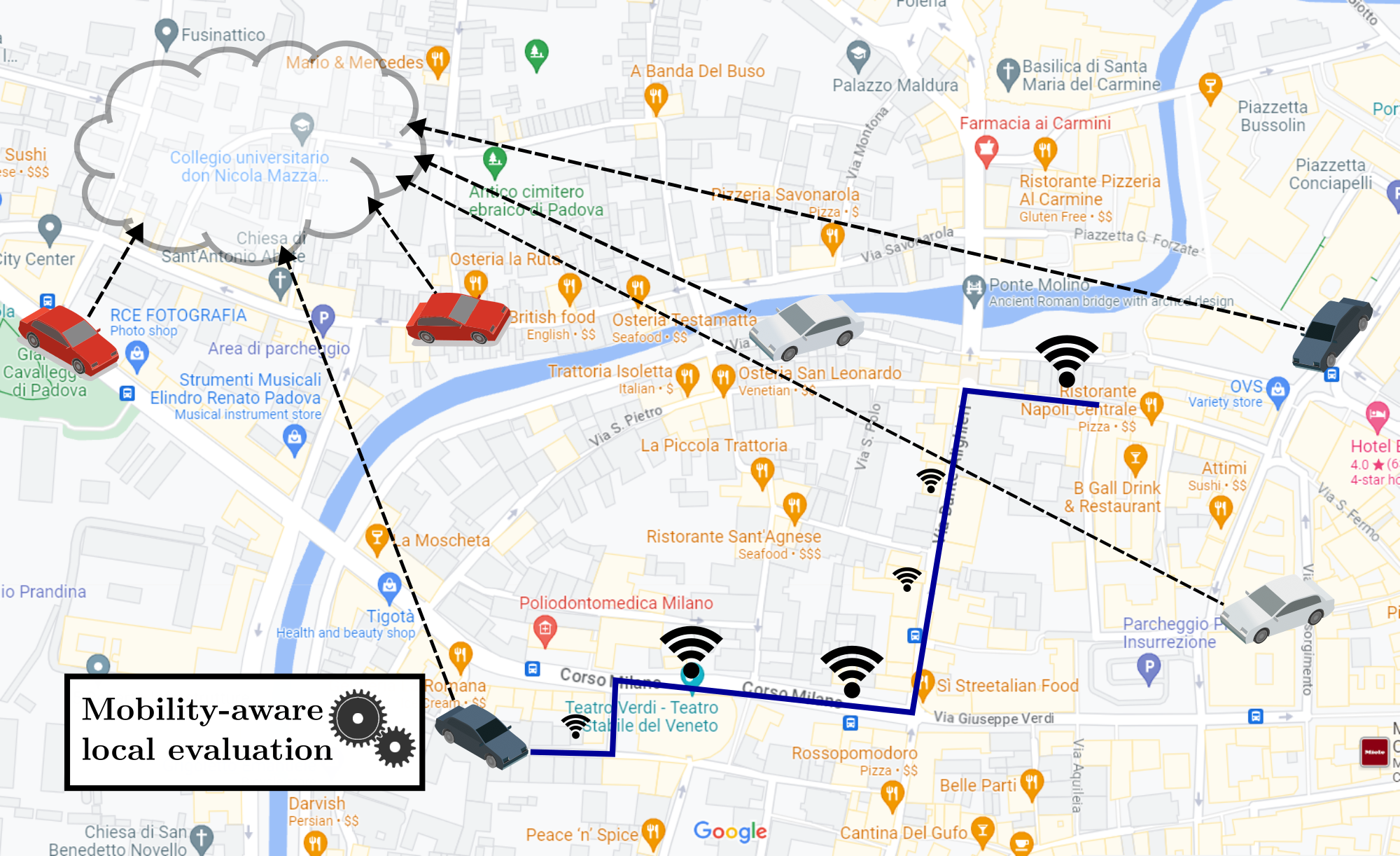
(b)

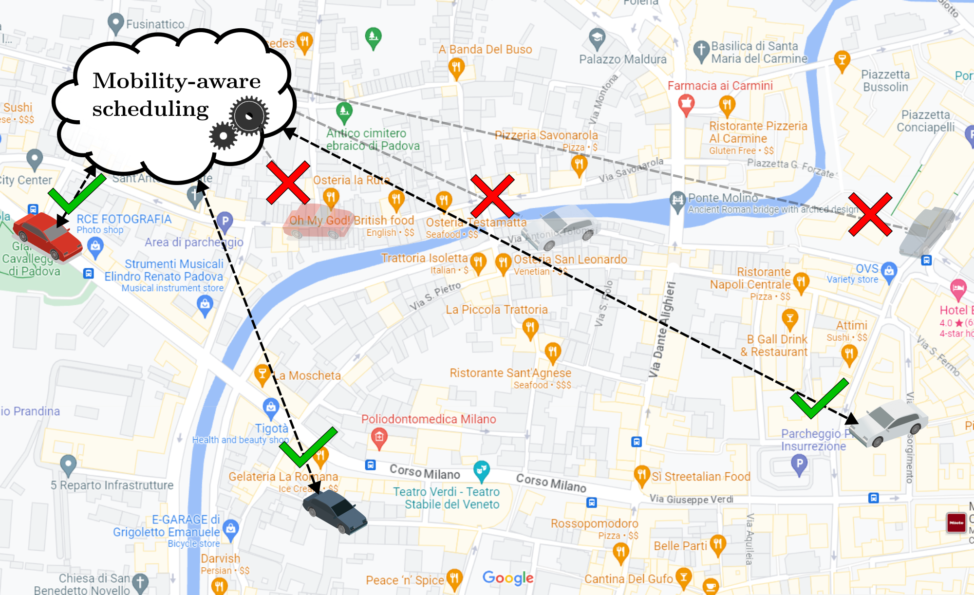
(c)

Fig. 1: VREM-FL. The mobility-aware co-design proposed in this article.

Among the most popular verticals of fifth generation (5G) and beyond communications, connected cars has the highest annual growth rate according to Cisco [cisco2020]. In 2021, Siemens estimated that the amount of data generated by autonomous vehicles will range from $3$ to $40$ $\mathrm{Gbit}$/$\mathrm{s}$ depending on the autonomy level [siemens2021avdata], which amounts to up to $19$ $\mathrm{TB}$ every hour.

The huge availability of data in modern vehicular networks paves the way to training, possibly at runtime, large deep learning models. Nowadays, this is mostly accomplished via federated learning (FL), which is the most prominent solution from the state-of-the-art to train neural networks from the data collected by distributed clients. FL has several advantages, such as high flexibility, offered by the possibility of choosing when local models are to be sent by the end users to the central aggregator, and offers a certain degree of privacy, due to the fact that end-user data is never transmitted: only the model weights are sent from the end-users to the aggregator.

Remarkably, despite the extensive amount of work available on communication-constrained [konevcny2016federated, mitra2021linear] and channel-aware [chen2020joint, chen2020convergence] FL algorithms, scheduling policies for vehicular networks that jointly consider mobility, communication/channel resources, and learning aspects are currently lacking.

In the present article, these aspects are jointly tackled for the first time, proposing vehicular radio environment map (REM) federated learning (VREM-FL), an FL scheduler that orchestrates the computation and the transmission of local models from the end users (the vehicles) to the central model aggregator (at the roadside network). VREM-FL exploits the availability of REMs to pick the most profitable transmission instants for the transmission of the local models from the vehicles. This is possible due to the fact that REMs are relatively stable over time [bi2019rem, dalfabbro2022rem], as they mainly depend on static obstacles, such as buildings in urban environments. Hence, their knowledge can be combined with information on the planned user routes to attain optimal FL transmission schedules. The optimization criteria correspond to minimizing the channel resources that are wasted due to transmitting when the channel conditions are poor, and to meeting a deadline for the global model update.

VREM-FL organizes the learning task into three stages, see Fig. 1 from top to bottom: (1) the central orchestrator, based on channel and computation resources, decides how many vehicles are allowed to participate in the current round, proposes an initial number of iterations for the update of their local models, and sets a maximal round latency (deadline); (2) all the vehicles, based on their private planned routes, learning metrics, and available REMs, adjust the number of local iterations received by the orchestrator, and decide when to transmit their own models; (3) the orchestrator, upon receiving the vehicles’ feedback, chooses the best subset of them to take part in the current round. The selected vehicles update their local models and send their model updates to the orchestrator. The received updates are finally used at the orchestrator to refine the global model.

Novel contributions

The main contributions of this article are summarized as follows.

• We propose VREM-FL, a computation-scheduling co-design tailored to vehicular FL. VREM-FL leverages the knowledge of vehicles’ routes and REMs, to optimize the communication resources used by the vehicles, while also ensuring high learning performance.

• A realistic simulation environment is implemented in Python using the street map of the city of Padova (Italy) and the popular simulator of urban environment (SUMO) [sumo]. On this map, base stations are deployed according to typical parameters of 5G cellular systems [grassi2018massive], to provide communications services to the vehicles. To capture realistic settings, where channel quality measurements are only available in a limited number of geographical locations, REMs are obtained via Gaussian process regression [dalfabbro2022rem, muppirisetty2015spatial].

• VREM-FL is evaluated via an extensive simulation campaign comprising (i) controlled experiments with a least squares (LS) toy example and (ii) a more realistic scenario involving the execution of a semantic segmentation task on the popular ApolloScape [huang2018apolloscape] dataset. Moreover, VREM-FL is compared with literature benchmarks such as vanilla federated averaging (FedAvg) [mcmahan2017] (i.e., random selection of clients) and the algorithm in [GunduzComputationTime], where a fairness metric for the selection of the vehicles is considered.

The rest of this paper is organized as follows. In Section II the state-of-the-art is presented; Section III provides a general overview of VREM-FL. In Section IV, the system model is presented, including the FL setup and the radio environment settings. The problem is defined in Section V, while VREM-FL is detailed in Section VI. Numerical simulation results demonstrating the effectiveness of VREM-FL are presented in LABEL:sec:results. Finally, conclusions are drawn in LABEL:sec:conclusion, along with future research directions.

II Related work

In this section, the state-of-the-art on FL over wireless networks is reviewed, focusing on the previous efforts on computation-communication co-design methods and on the existing solutions for vehicular FL. Some relevant approaches to leverage REMs for wireless resource management are also discussed, underlining the novelty of our solution.

II-A User scheduling for FL in wireless networks

Lately, many research works have investigated scheduling techniques for FL over wireless networks [TWC_wirelessFL_SCH_WN4, SAC_WN2Edge, CDC_submodular_WN3, DeviceSchedWN1, IoTBudget]. In [SchedulingPoor], scheduling policies were experimented with by simulating users connected to different access points together with different signal-to-interference-plus-noise ratio (SINR) thresholds. The recent work [PALORA] proposed PALORA, a scheduling method jointly considering fairness with respect to the local models, signal-to-noise ratio (SNR) levels, and resource blocks utilization. Along the same lines, the paper [GunduzComputationTime] considered asynchronous updates, took into account the computation-communication tradeoff, and proposed scheduling strategies based on age-of-information (AoI) and fairness. This paper presented experiments with realistic FL training time estimates over wireless networks. In [DataQuality], scheduling was performed based on data quality metrics establishing a user priority indicator, which is used to jointly solve a user selection and bandwidth allocation problem. A scheduling approach based on data selection was proposed in [SchedGradientNormDataSel], where the gradient norm was used to compute a metric that relates learning efficiency with data selected by users for local training. The authors of [WCLs_chAndLearnSched] proposed a scheduling policy for FL over an orthogonal frequency-division multiple access (OFDMA) scheme where scheduling decisions are based on learning accuracy and channel quality.

II-B FL in vehicular networks

There is a growing interest in machine learning solutions for problems related to vehicular networks, given the increasing need for data-driven algorithms in intelligent transportation systems [TowardsIntelligentVNs_ML]. Applications examples include wireless resource management [RadioResourceAlloc], traffic flow prediction [TrafficFlowPrediction], vehicle-based perception for autonomous driving [FL_IoT_IoVs, AutonomousFL_Conf], to name a few.

With respect to the federated training setup, some works have focused on static vehicular federated learning [Static_1_Survey, Static_2Approach], with particular emphasis on scenarios involving parking lots [Static_3PLs] and related issues, like parking space estimation.

Conversely, cooperative training of machine learning models in scenarios involving user mobility, as in vehicular networks, is still an open and key research objective [SurveyHighMobility, VehFL_bennis]. In this context, several works have recently considered vehicular FL for, e.g., image classification problems [ImageFLMobility], proactive caching [proactiveCaching], and object detection [ObjectDetection6G].

Recently, other works have investigated the allocation and optimization of network resources in vehicular FL [FL_veh_opt_1, FL_veh_opt_2, FL_veh_opt_3, FL_veh_opt_4, FL_veh_opt_5]. Specifically, the work [FL_veh_opt_3] analyzed the impact of vehicular mobility on wireless transmissions, proposing wireless network optimization techniques to improve the performance. The authors of [FL_veh_opt_5] considered cache queue optimization at the edge server, while other related scheduling techniques were proposed in [FL_veh_opt_1, FL_veh_opt_2]. On the other hand, the authors of [FL_veh_opt_4] focused on tuning the number of local iterations based on mobility awareness in relation to short-lived connections with the base stations. The work [SchedResourceAlloc] studied the adoption of FL in an IoV scenario where vehicles communicate with 5G base stations, exploiting context information such as cell association and mobility prediction together with the related channel quality for users’ scheduling.

However, none of the above-mentioned works leverages the combination of mobility patterns and radio environmental awareness to optimize the learning performance of federated learning while at the same time optimizing wireless network resources. Our work is the first to jointly consider these aspects which, as we shall see, leads to sizeable advantages over previous solutions.

II-C REMs for wireless resource management

A radio environment map (REM) is a geographic database of average communication quality metrics. In recent years, REMs have been proposed as an effective tool to manage wireless resources [bi2019rem]. For example, REMs have been advocated for predictive resource allocation [predictiveREM] and handover management in 5G networks [handoverREM]. Recently, in 5G systems with massive multiple-input multiple-output (mMIMO) transmission, REMs have been adopted for energy efficient design [energyREM], inter-cell interference coordination [chikha2022radio], beam management [beamManagementREM], and cell-edge users throughput improvement via dynamic point blanking [throughputREM]. Even though the use of REMs has been investigated for several resource management applications in wireless communications, this work is the first to exploit them for network resources optimization in FL and, specifically, in vehicular FL.

III VREM-FL in a nutshell

In this article, we are concerned with optimal resource allocation for FL tasks executed by vehicles traveling within an urban environment and an edge server acting as a centralized aggregator of the model. In what follows, we interchangeably use the terms “vehicle” and “client” depending on the role that we would like to emphasize.

III-A The problem: resource allocation for vehicular FL

We aim to minimize the objective

$$\mathrm{cost} =\mathrm{training\ loss}+\mathrm{overall\ latency}$$ (OBJ)

$$\quad+\mathrm{channel\ usage}$$

associated with an FL task, where the $\mathrm{training\ loss}$ measures the performance (accuracy) of the globally learned model, the $\mathrm{overall\ latency}$ is the total time used to train the model, and the $\mathrm{channel\ usage}$ refers to the time during which the channel is used to transmit the local models from the clients.

The space of intervention that we consider encompasses three aspects. The first one concerns scheduling the clients during training. Due to the limited nature of communication and computation resources, it is typically infeasible for all the clients to transmit their local model at every learning round. For this reason, they need to be scheduled: at each learning round, only a subset of them is selected. A scheduling strategy is thus required to optimally choose which clients should update the global model at every round.

The second aspect is the amount of local computation performed by the scheduled clients (vehicles). To ensure convergence of an FL algorithm to an accurate global model, the clients must carefully choose how many stochastic gradient descent (SGD) steps to perform when updating their local model. Under client scheduling, and if the clients independently choose their number of local steps at each round, optimally tuning the number of such local steps is challenging because of the combinatorial nature of the associated optimization problem.

The third aspect that we optimize for is the transmission of local models from the vehicles to the edge server. In general, sending the updated local models as soon as the local computations are performed (greedy behavior) would yield the fastest training. However, this strategy does not take into account the channel status, which depends on mobility and radio channel dynamics. It descends that a greedy transmission behavior is not necessarily optimal in terms of making the best possible use of the available channel resources. The proposed policy is mobility and channel aware; through its use, channel resources are more profitably exploited. This leads to benefits in terms of reduced transmission energy and additional room for other users or tasks that also need to exploit wireless transmissions.

III-B The solution: VREM-FL

To minimize the cost (OBJ) in a vehicular scenario, we propose Vehicular REM-based Federated Learning (VREM-FL), a co-design that jointly optimizes the threefold decision-making introduced above. An intuitive description of our co-design algorithms is illustrated in Fig. 1. In this section, we provide a high-level overview of how VREM-FL works and defer the detailed explanation to Section VI.

VREM-FL is run at the beginning of each learning round and consists of three phases, which correspond to the boxes in Fig. 1.

During the centralized optimization phase (top box), the edge server (i.e., the orchestrator) computes the number of local steps that all the vehicles should perform to achieve the fastest training convergence and broadcasts this information. This computation uses a proxy for global convergence assuming that all the scheduled vehicles run the same number of local steps [li2019convergence]. Hence, the server does not need to know the vehicles’ local cost functions. This phase is formalized in Section VI-A.

In the local customization phase (middle box), each vehicle adjusts the number of local steps based on a local convergence criterion to trade local training speed for global accuracy. Hence, the vehicle optimizes the communication of the local model by opportunistically delaying its transmission, seeking the best trade-off between the cost components $\mathrm{overall\ latency}$ and $\mathrm{channel\ usage}$, see (OBJ). To perform this optimization, the vehicle leverages knowledge of (i) the channel quality via the availability of an estimated REM and (ii) its planned trajectory, as explained in Section VI-B. No training is performed at this stage: instead, the choice of computation and communication is used in the following phase to discern which vehicles are the best candidates to be scheduled at the current round.

Finally, in the centralized scheduling phase (bottom box), the edge server receives from all the vehicles their estimated costs for participating in the round. These costs depend on the local decision-making performed during the previous phase and are suitably combined with global information available at the server, which measures the fairness of updates among the vehicles. The latter element, in the form of a combination of AoI and scheduling frequency metrics, ensures appropriate participation of all the vehicles throughout the training. The algorithm executed at the server to make scheduling decisions is described in LABEL:sec:centralized-problem-2.

IV System Model

In this section, we present the setup considered throughout the article. In Section IV-A, we introduce an FL task solved by vehicles that move within an urban environment served by edge servers. In Section IV-B, we describe the model that expresses channel quality experienced by the vehicles, that they use to locally assess whether they should join a round and optimize their subsequent transmissions to the server.

IV-A Vehicular federated learning

We consider $N$ vehicles that move within an urban environment. The set of all vehicles is denoted by $\mathcal{V}\doteq\{1,\dots,N\}$, and a vehicle in this set is referred to as $v\in\mathcal{V}$. The mobility area is served by $N_{\text{bs}}$ 5G BSs. As vehicles travel, they collect data to improve the efficiency of the tasks of interest, such as the semantic segmentation of the surrounding environment for local navigation or some global route optimization based on real-time traffic information. We label the local dataset of vehicle $v$ as $\mathcal{D}_{v}$. To efficiently learn complex tasks from locally gathered data, all vehicles in $\mathcal{V}$ are connected to an edge server running an FL algorithm. This allows different vehicles to cooperatively learn a common machine learning (ML) model without having to upload the collected data to the server, which may be impractical due to the high data volume or undesirable due to privacy concerns.

The FL task is described by the following optimization problem: θ_,^ ∈Θ L(θ_,^ ) ≐ℓ(θ_,^ ;{D_v}_v∈V_)+ λ∥θ_,^ ∥ where $\theta_{{},{}}$ is the model parameter, function $\ell(\cdot;\cdot)$ is the empirical loss that depends on the dataset, norm $\left\lVert\theta_{{},{}}\right\rVert$ is a regularization term that, in words, penalizes “complex” models, and $\lambda$ is the regularization weight. In the following, we refer to the total cost $\mathcal{L}(\theta_{{},{}})$ as (regularized) loss for the sake of simplicity. Also, the size of the parameter $\theta_{{},{}}$ amounts to $B$ [$\mathrm{bit}$].

While our co-design algorithms are agnostic to the specific algorithm used to solve problem (IV-A), in the following, we assume that the edge server runs FedAvg [mcmahan2017] and that the vehicles train their local models via gradient descent (GD) or SGD, to ground the discussion. A high-level snippet of vanilla FedAvg (without client scheduling) is provided in Algorithm 1, where all clients perform $H$ SGD steps for each local update. We refer to a cycle composed of local updates and global aggregation (Algorithms 1, 1, 1, 1 and 1) as a (learning) iteration or (learning) round, whose duration coincides with the time interval between two consecutive updates of the global model, and assume that the edge server runs FedAvg for $T$ rounds in total. Moreover, we denote the global parameter at iteration $t$ by $\theta_{{},{}}^{t}$, while the locally updated parameter of vehicle $v$ during round $t$ (before transmission to the aggregator) is denoted by $\theta_{v,t+H}^{t}$.

As commonly done in the literature, we further assume that each learning iteration has a deadline after which the global aggregation is executed regardless of the status of local updates, and a new learning round begins afterward. Also, time is slotted into slots of duration $\tau$ [$\mathrm{s}$], which we consider the finest granularity to allocate resources in a time-varying fashion. In our present work, local training (Algorithm 1) and transmission of local models from the vehicles to the server (Algorithm 1) are addressed: we further assume that the vehicles have a deadline of $K_{\text{max}}$ [$\mathrm{s}$] to update their local models and to upload them to the server at every round, corresponding to $\lfloor K_{\text{max}}/\tau\rfloor$ time slots. We denote the set of time slots available during iteration $t$ by $\mathcal{K}_{t}$. In the following, we will refer to the local training performed by the vehicles as computation to highlight the allocation of computational resources.

Input: Loss $\mathcal{L}$, rounds $T$, parameter $\theta_{{},{}}^{0}$, local steps $H$.

Output: Learned parameter $\theta_{{},{}}^{t}$.

1 for $t=0,1,\dots,T$ do

2       server broadcasts global parameter $\theta_{{},{}}^{t}$ to vehicles;

3       foreach vehicle $v\in\mathcal{V}$ do

4             train local model: $\theta_{v,t+H}^{t}\leftarrow\mathrm{SGD}\left(\theta_{{},{}}^{t},H;\mathcal{D}_{v}\right)$;

5             transmit local parameter to server;

6            

7      server aggregates local models: $\theta_{{},{}}^{t+1}\leftarrow\sum_{v\in\mathcal{V}}w_{v}\theta_{v,t+H}^{t}$;

8      

Algorithm 1 Vanilla FedAvg [mcmahan2017]

Remark 1 (Performing FL on traveling vehicles).

The related literature [siemens2021avdata, 1GBPerSecIntelligent] remarks that the sensing capabilities of autonomous vehicles may generate $\mathrm{GB}$s of data per second. The cost for such a massive amount of data is high in terms of energy consumption and storage capacity. Hence, besides the possible need to learn a model as they travel, the vehicles may destroy the collected data right after using it for training, to save memory. Conversely, running the FL task on idle vehicles after they have collected all data imposes high, if not impractical, storage requirements and energy consumption.

IV-B Radio environment and Bitrate

The area served by the BSs features a heterogeneous channel quality depending on the network coverage at different geographical locations. An REM is a database that links a (quantized) geographical location to the (estimated) value of some channel quality metric. In this work, we are interested in utilizing the knowledge of the average bitrate associated with a location $x\in{{\mathbb{R}}^{2}}$. We consider an REM that contains information about the SINR experienced on average across space. Given a wireless transmission setting and a geographical location $x$, the value of the SINR associated with $x$ contained in the REM can be used to infer the expected average bitrate experienced by a user located at $x$. This information is crucially used for resource orchestration by VREM-FL. Formally, we express the location-to-bitrate map as follows. Given a vehicle $v$ located at $x_{t}^{v}$ at time $t$, the corresponding estimated average bitrate $h_{t}^{v}$ is

$$h_{t}^{v}=\beta(\gamma(x_{t}^{v}),\eta_{t}^{v}),$$ (1)

where $\gamma(\cdot)$ is the location-to-SINR map encoded by the REM, $\beta(\cdot)$ is the SINR-to-bitrate map, and $\eta_{t}^{v}$ is the bandwidth used by vehicle $v$ at time $t$. Without loss of generality, in the rest of the paper, we set $\eta_{t}^{v}=\eta$, constant and identical for all vehicles.

In practice, we assume that an REM of the environment is computed a priori by means of some estimation technique [sato2017kriging, sato2021space, chowdappa2018distributed] and is deployed at the edge server that broadcasts this information to the vehicles. Because REMs are approximately constant over time, as previously mentioned, we assume that an REM is sent to the vehicles only once before the FL training.

As they travel, vehicles may experience a different channel quality according to their location. We assume that the routes traversed by the vehicles are planned in advance (at least partially) so that they know their trajectory in the near future at each point in time. Specifically, at time $t$, vehicle $v$ knows the locations it is about to traverse over the next $D$ time instants, denoted by $x_{t}^{v},\dots,x_{t+D}^{v}$, for some suitable time horizon $D$. This geographical information can be converted to the average bitrate experienced by the vehicle along its planned trajectory as per (1), resulting in $h_{t}^{v},\dots,h_{t+D}^{v}$, where $h_{k}^{v}=\beta\left(\gamma(x_{k}^{v}),\eta\right)$. This information is used in our resource-allocation algorithms, as detailed in Section V.

V Problem formulation

We now formalize the computation-scheduling co-design problem that is the core of our novel contribution: we first define the design parameters corresponding to the considered decision-making (Section V-A), and then formally write the objective function (OBJ) along with the overall optimization problem (Section V-B).

V-A Design parameters

Given problem (IV-A) and an algorithm to solve it (FedAvg), we are concerned with the threefold decision-making associated with the algorithm workflow discussed in Section III-A, which is our space of intervention.

V-A1 Scheduling

First, we design a scheduling strategy to select the vehicles that participate in each learning iteration. Scheduling is needed because the total amount of vehicles involved in an FL task is typically large and cannot be handled at once due to the limited communication resources available at the BSs. It descends that only a (small) fraction of the vehicles can be simultaneously served through the available bandwidth to ensure an acceptable quality of service. We denote the subset of vehicles that participate in round $t$ by $\mathcal{V}_{t}^{S}\subset\mathcal{V}$ and the maximum number of vehicles that can be scheduled in round $t$ by $M_{t}^{S}<N$, with $\lvert\mathcal{V}_{t}^{S}\rvert\leq M_{t}^{S}$.

V-A2 Computation

For each vehicle scheduled in a learning round, we consider two aspects for co-design. First, we allocate the amount of computation at the vehicle, that is, the number of descent steps (of GD or SGD) that the vehicle performs during that round to train the local model. Through a careful choice of the number of local steps, we can effectively trade convergence speed of FedAvg for the quality of the final global model. For each time slot $k\in\mathcal{K}_{t}$ available during iteration $t$, we denote by $a_{k}^{v}\in\{0,1\}$ the computation decision of vehicle $v$ for slot $k$: if $a_{k}^{v}=1$, it means that $v$ performs a batch of local steps during slot $k$, otherwise no computation is carried out in that slot. All slots used by vehicle $v$ for local training during round $t$ are denoted by $T_{\text{cpu},t}^{v}\doteq\sum_{k\in\mathcal{K}_{t}}a_{k}^{v}$. To make the training meaningful, we allocate at least $T_{\text{cpu}}^{\text{min}}\geq 1$ slots for computation at every round.

V-A3 Communication

After a vehicle has updated its local model, we optimize the transmission from vehicle to server. Although the training time for FL is trivially minimized if local models are immediately transmitted, in this work we are additionally interested in an efficient allocation of network resources. This allows us to save on the number of slots during which the channel bandwidth is reserved for FL and also to reduce the transmission energy. In particular, we assume that all vehicles have a constant transmission power so that optimizing for communication resources is equivalent to transmitting where the SINR is high. Similarly to computation decisions, we denote by $b_{k}^{v}\in\{0,1\}$ the transmission decision of vehicle $v$ in slot $k$: if $b_{k}^{v}=1$, it means that $v$ uses channel slot $k$ to transmit its local model to the server, otherwise no transmission occurs during that slot. The total time used by vehicle $v$ to transmit its local model during round $t$ is denoted by $T_{\text{tx},t}^{v}\doteq\sum_{k\in\mathcal{K}_{t}}b_{k}^{v}$. Further, we denote by $K_{t}^{v}$ the total amount of time elapsed from the beginning of the local model update to the end of its transmission to the server, which we refer to as round latency of vehicle $v$.

Fig. 2: Workflow of VREM-FL. At the beginning of learning iteration $t$, the server runs centralized optimization and transmits the globally optimal local steps to the clients. Then, each vehicle locally runs local customization to fine-tune computation and communication resources to be used in the round. Finally, the server performs centralized scheduling taking into account both feedback from the vehicles and global participation information.

V-B Optimization problem

We aim to jointly optimize the three potentially contrasting objectives in (OBJ). As discussed above, the optimization of computation and scheduling resources enhances the final $\mathrm{training\ loss}$ and $\mathrm{overall\ latency}$ of the FL task, while optimizing communication resources translates into an efficient $\mathrm{channel\ usage}$ during training. We now formally express these concurrent costs highlighting the dependency on the design parameters.

With a slight abuse of notation, we express the $\mathrm{training\ loss}$ as a function of both computation and scheduling (note that it also depends on the final parameters learned by FedAvg, $\theta_{{},{}}^{T}$):

$$\mathrm{training\ loss}=\mathcal{L}\left(\left\{\mathcal{V}_{t}^{S},\{a_{t}^{v}\}_{v\in\mathcal{V}_{t}^{S}}\right\}_{t\in\mathcal{T}};\theta_{{},{}}^{T}\right),$$ (TL)

where $a_{t}^{v}\doteq\left\{a_{k}^{v}\right\}_{k\in\mathcal{K}_{t}}$ denotes all the computation decisions of vehicle $v$ throughout round $t$ and the set $\mathcal{T}\doteq\{1,\dots,T\}$ gathers all learning rounds. The $\mathrm{overall\ latency}$ is upper bounded by $TK_{\text{max}}$ but can vary depending on (i) how computation and communication resources are allocated, and (ii) the channel quality experienced by the scheduled vehicles. We formalize this as

$$\mathrm{overall\ latency}=K\left(\left\{\left\{a_{t}^{v},b_{t}^{v};h_{t}^{v}\right\}_{v\in\mathcal{V}_{t}^{S}}\right\}_{t\in\mathcal{T}}\right),$$ (OL)

where $b_{t}^{v}\doteq\left\{b_{k}^{v}\right\}_{k\in\mathcal{K}_{t}}$ and $h_{t}^{v}\doteq\left\{h_{k}^{v}\right\}_{k\in\mathcal{K}_{t}}$ denote all the transmission decisions of vehicle $v$ and bitrate values experienced by $v$ during round $t$, respectively. Finally, we quantify the $\mathrm{channel\ usage}$ as the time (number of slots) in which vehicles reserve the channel bandwidth to upload their local models to the server. Since this quantity depends on both the transmission decisions and the bitrate, we write it as

$$\mathrm{channel\ usage}=\sum_{t\in\mathcal{T}}\sum_{v\in\mathcal{V}_{t}^{S}}T_{\text{tx},t}^{v}\left(b_{t}^{v};h_{t}^{v}\right).$$ (CU)

The total cost (OBJ) addressed in our co-design amounts to

$$\begin{split}\mathrm{cost}\left(\mathcal{V}^{S},a,b;h,\theta_{{},{}}^{T}\right)&=\begin{aligned} &\mathcal{L}\left(\mathcal{V}^{S},a;\theta_{{},{}}^{T}\right)\\ &+(1-w_{\mathrm{tx}})K\left(a,b;h\right)\\ &+w_{\mathrm{tx}}\sum_{t\in\mathcal{T}}\sum_{v\in\mathcal{V}_{t}^{S}}T_{\text{tx},t}^{v}\left(b_{t}^{v};h_{t}^{v}\right)\end{aligned}\end{split}$$ (2)

where $\mathcal{V}^{S}\doteq\{\mathcal{V}_{t}^{S}\}_{t\in\mathcal{T}}$ denotes the full client schedule, $a\doteq\{\{a_{t}^{v}\}_{v\in\mathcal{V}_{t}^{S}}\}_{t\in\mathcal{T}}$, $b\doteq\{\{b_{t}^{v}\}_{v\in\mathcal{V}_{t}^{S}}\}_{t\in\mathcal{T}}$, and $h\doteq\{\left\{h_{k}^{v}\right\}_{k\in\mathcal{K}_{t}}\}_{t\in\mathcal{T}}$ collect all the computation and transmission decisions, and bitrate values associated with the scheduled vehicles across rounds. The weight $w_{\mathrm{tx}}\in[0,1]$ trades $\mathrm{overall\ latency}$ (OL) for $\mathrm{channel\ usage}$ (CU): if $w_{\mathrm{tx}}=0$, only the training time is penalized in (2); if $w_{\mathrm{tx}}=1$, latency is not addressed, but the usage of network resources is discouraged. Note that the performance term (TL) and the latency cost (OL) in (2) jointly depend on all scheduled clients, whereas the resource-related cost (CU) decomposes linearly across them.

Equipped with the mathematical definition (2) of (OBJ), we are now ready to formalize the computation-scheduling co-design problem tackled in the rest of this work.

TABLE I: List of symbols used in this article.

$\mathcal{V}$	set of vehicles
$B\leavevmode\nobreak\ [$\mathrm{bit}$]$	size of model parameter $\theta$
$\tau\leavevmode\nobreak\ [$\mathrm{s}$]$	duration of one time slot
$K_{\text{max}}\leavevmode\nobreak\ [$\mathrm{s}$]$	maximum latency of every learning iteration
$T_{\text{cpu}}^{\text{min}}$	minimum number of computation slots at every iteration
$\mathcal{K}_{t}$	set of time slots available for iteration $t$
$s_{v}$	local steps that vehicle $v$ runs in one time slot
$a_{k}^{v}$	computation decision of vehicle $v$ for slot $k$
$b_{k}^{v}$	transmission decision of vehicle $v$ for slot $k$
$T_{\text{cpu},t}^{v}$	number of computation slots of vehicle $v$ in iteration $t$
$T_{\text{tx},t}^{v}$	number of transmission slots of vehicle $v$ in iteration $t$
$h_{k}^{v}\leavevmode\nobreak\ [$\mathrm{bit}$/$\mathrm{s}$]$	bitrate experienced by vehicle $v$ in slot $k$
$B_{t}^{v}\leavevmode\nobreak\ [$\mathrm{bit}$]$	bits that vehicle $v$ transmits during iteration $t$
$K_{t}^{v}\leavevmode\nobreak\ [$\mathrm{s}$]$	latency of vehicle $v$ in iteration $t$
$\mathcal{V}_{t}^{S}$	set of vehicles scheduled for iteration $t$
$M_{t}^{S}$	maximum number of vehicles scheduled for iteration $t$

Problem 1 (Optimal computation-scheduling co-design for vehicular FL).

Given (i) a set of vehicles $\mathcal{V}$, (ii) an REM of the environment $\gamma$, (iii) an FL algorithm, (iv) model parameters $B,K_{\text{max}},T_{\text{cpu}}^{\text{min}}$, find (1) a vehicle schedule $\mathcal{V}^{S}$, (2) computation decisions $a$, (3) transmission decisions $b$, so as to optimize FL training and transmission resources: V_^S,a_^,b_^ cost(V_^S,a_^,b_^;h,θ_,^T ) (P)   K_t^v≤K_max ∀v∈V_t^S, t∈T T_cpu,t^v≥T_cpu^min  ∀v∈V_t^S,t∈T. In words, constraint (1) ensures that each round ends within the pre-assigned deadline, and constraint (1) requires the scheduled vehicles to perform a minimal number of descent steps. The meaning of all symbols is provided in Table I.

In the next section, we propose co-design algorithms to solve 1 that crucially rely on vehicular mobility and the REM to estimate the channel quality experienced by vehicles.

VI Algorithms for co-design

The computation-scheduling co-design problem (P) requires designing both the local operations performed by the vehicles (computation and transmission) and the global scheduling decisions the edge server makes (the selection of which vehicles contribute in the current round). To efficiently tackle it, we propose a cascade procedure that is executed at the beginning of each round $t$, involving three phases (split between the edge server and the vehicles).

Centralized optimization:

the edge server computes the optimal number of local steps $H_{t}^{*}$ to be performed by the vehicles in round $t$ and broadcasts them this value.

Local customization:

the vehicles locally customize their number of local steps and their transmission pattern (the channel slots to use for sending their local model update), and send back to the server their predicted cost $C_{t}^{v}$ to participate in round $t$.

Centralized scheduling:

the server receives all the costs $C_{t}^{v}$ and uses both such local information and global knowledge about the fairness of updates to select the subset of vehicles that will actually take part in the model update at round $t$.

Figure 2 provides a schematic representation of the workflow of VREM-FL with the three phases listed above. In the following, the operations of VREM-FL are described in detail.

VI-A Centralized optimization

In this phase, the edge server first sets the maximum number $M_{t}^{S}$ of vehicles that are allowed to participate in round $t$ based on its available local resources (e.g., transmission channel resources and computational capability for model aggregation). Then, the server computes an approximate number of local steps to be performed by the scheduled vehicles in order to speed up the training. To evaluate at runtime the relation between the number of local steps at the vehicles and the training time, we use the proxy for global FL convergence proposed in [li2019convergence, Eq. (1)]. This proxy assumes that $M$ clients are scheduled at every round, and that each of them performs $H$ local steps at every local update. The proxy is expressed as

$$T\epsilon\approxeq\Gamma(H,M)\doteq\frac{C}{H}+\left(1+\frac{1}{M}\right)H$$ (GP)

where $\epsilon$ is the estimated accuracy in $T$ rounds, i.e., $\mathcal{L}(\theta_{{},{}}^{T})\leq\epsilon$, and $C$ is a constant that depends on the data distribution.

The server homogeneously chooses $H_{t}^{*}$ as the minimizer of the proxy (GP) with respect to $H$, setting $M=M_{t}^{S}$ and assuming that all vehicles run $H_{t}^{*}$ local steps at all iterations: H Γ(M_t^S,H). H_t^*= This first unconstrained subproblem is convex because the objective cost (GP) is convex in $H$. Its solution, attainable in closed form, is

$$H_{t}^{*}=\sqrt{\frac{C}{\left(1+\frac{1}{M_{t}^{S}}\right)}}.$$ (3)

This also reveals the dependency of the optimal number of local steps $H_{t}^{*}$ on the number of scheduled clients: it is a strictly increasing and concave function of $M$ (for $M\geq 1$) which saturates to $\sqrt{C}$ for $M\to+\infty$ (horizontal asymptote).

After computing $H_{t}^{*}$, the server broadcasts this value to all the vehicles for the second phase.

VI-B Local customization

Fig. 3: Behavior of a selected client at each round. If a client $v$ is selected by the server, it goes through the following steps. Each slot has duration $\tau$ [$\mathrm{s}$]. At first, the client performs some local (S)GD steps (computation) according to its computation allocation. Eventually, it transmits its updated local model (transmission) after time $K_{t}^{v}$ and within the maximum allowed latency $K_{\text{max}}$, possibly waiting for some time slots (idle) to enjoy a better channel quality.

In this phase, each vehicle independently executes a local subroutine to allocate slots for computation and communication. This allocation attempts to optimize (i) convergence of local training and (ii) channel utilization. The resulting number of local steps is temporarily stored by the vehicles, which use it later to perform the local model update in case they are actually scheduled. If a vehicle has a means to (efficiently) estimate the loss gradient, it first refines the number of local steps $H_{t}^{*}$ communicated by the server (computation refinement) based on a proxy for local convergence, obtaining a new number of local steps $H_{t}^{v}$, and then it optimizes for transmission (communication optimization). Instead, if evaluating the gradient is expensive, the vehicle skips the computation refinement at this stage and sets the number of local steps as $H_{t}^{v}=\max\left\{H_{t}^{*},s_{v}T_{\text{cpu}}^{\text{min}}\right\}$.

VI-B1 Computation refinement

To optimize the local updates of the vehicle, we consider a local proxy that jointly keeps into account the individual client convergence properties and the global recommendation $H_{t}^{*}$ indicated by the server. As such, the proxy is obtained as the sum of multiple terms. First, we consider a "convergence" proxy $\Theta^{v}_{t}\left(H_{t}^{v}\right)$ related to the local optimality gap, which bounds the client deterministic gradient norm after $H_{t}^{v}$ local steps of gradient descent starting from the global parameter $\theta_{{},{}}^{t}$:

$$\left\lVert\nabla\ell^{v}\!\left(\theta_{v,t+H_{t}^{v}}^{t}\right)\right\rVert\leq\Theta^{v}_{t}\left(H_{t}^{v}\right)\doteq\left\lVert\nabla\ell^{v}\!\left(\theta_{{},{}}^{t}\right)\right\rVert\!\left(1-\kappa_{v}^{-1}\right)^{H_{t}^{v}-1}.$$ (LP)

The constant $\kappa_{v}>0$ is the condition number associated with the local loss $\ell^{v}$. The proxy (LP) is based on quadratic cost functions, and we derive it explicitly in Appendix LABEL:app:proxy. The proxy (LP) is motivated by the fact that the optimality gap $\|\theta-\theta^{*}\|$ is in general proportional to the gradient norm, but we have only access to the gradient, while $\theta^{*}$ is unknown. It can be computed by each client based on their local cost only and does not take into account the distributed nature of the FL problem. Hence, during this step, the vehicle $v$ refines its computation by solving the optimization problem H∈N Θ^v_t(H)+