First-Order Model Checking on
Monadically Stable Graph Classes

Abstract

A graph class $\mathscr{C}$ is called monadically stable if one cannot interpret, in first-order logic, arbitrary large linear orders in colored graphs from $\mathscr{C}$. We prove that the model checking problem for first-order logic is fixed-parameter tractable on every monadically stable graph class. This extends the results of [Grohe, Kreutzer, and Siebertz; J. ACM ’17] for nowhere dense classes and of [Dreier, Mählmann, and Siebertz; STOC ’23] for structurally nowhere dense classes to all monadically stable classes.

This result is complemented by a hardness result showing that monadic stability is precisely the dividing line between tractability and intractability of first-order model checking on hereditary classes that are edge-stable: exclude some half-graph as a semi-induced subgraph. Precisely, we prove that for every hereditary graph class $\mathscr{C}$ that is edge-stable but not monadically stable, first-order model checking is $\mathrm{AW}[*]$-hard on $\mathscr{C}$, and $\mathrm{W}[1]$-hard when restricted to existential sentences. This confirms, in the special case of edge-stable classes, an on-going conjecture that the notion of monadic NIP delimits the tractability of first-order model checking on hereditary classes of graphs.

For our tractability result, we first prove that monadically stable graph classes have almost linear neighborhood complexity. We then use this result to construct sparse neighborhood covers for monadically stable graph classes, which provides the missing ingredient for the algorithm of [Dreier, Mählmann, and Siebertz; STOC 2023]. The key component of this construction is the usage of orders with low crossing number [Welzl; SoCG ’88], a tool from the area of range queries.

For our hardness result, we first prove a new characterization of monadically stable graph classes in terms of forbidden induced subgraphs. We then use this characterization to show that in hereditary classes that are edge-stable but not monadically stable, one can effectively interpret the class of all graphs using only existential formulas.

20(-1.75, 0.9) 20(-1.75, 1.9)

1 Introduction

We study the model checking problem for first-order logic on graphs: given a first-order sentence $\varphi$ in the vocabulary of graphs (consisting of one binary adjacency relation $E(\cdot,\cdot)$) and a graph $G$, decide whether $\varphi$ holds in $G$. Arguably, this is the most fundamental problem of algorithmic model theory, and it can be used to model many concrete problems of interest. For instance, the following two sentences express that the graph in question contains a clique of size $k$ or a dominating set of size $k$, respectively.

$$\exists x_{1}\ldots\exists x_{k}\ \bigwedge_{1\leqslant i<j\leqslant k}E(x_{i},x_{j})\qquad\qquad\qquad\exists x_{1}\ldots\exists x_{k}\forall y\ \bigvee_{1\leqslant i\leqslant k}(y=x_{i})\vee E(y,x_{i})$$

Clearly, first-order model checking can be solved by brute-force in time $n^{\mathcal{O}(\|\varphi\|)}$ on $n$-vertex graphs. However, as the problem is $\mathrm{AW}[*]$-hard, we cannot expect a fixed-parameter tractable algorithm, that is, an algorithm with a running time of the form $f(\|\varphi\|)\cdot n^{c}$ for a computable function $f$ and constant $c$, unless $\mathrm{FPT}=\mathrm{AW}[*]$ and the whole hierarchy of parameterized complexity classes collapses. Therefore, significant effort has been devoted to understanding on which restricted classes of graphs first-order model checking is fixed-parameter tractable, as well as finding the dividing line between tractability and intractability. Despite decades of intensive studies, a comprehensive understanding of the answer to this question has not yet been achieved.

A landmark result in this area is the following theorem of Grohe, Kreutzer, and Siebertz [GKS17]: If a graph class $\mathscr{C}$ is nowhere dense, then the first-order model checking problem on $\mathscr{C}$ can be solved in time $f(\|\varphi\|,\varepsilon)\cdot n^{1+\varepsilon}$, for any $\varepsilon>0$. Here, nowhere denseness is a structural property of a graph class that turns out to be precisely the dividing line for subgraph-closed classes: if a subgraph-closed class of graphs $\mathscr{C}$ is not nowhere dense, then model checking on $\mathscr{C}$ is as hard as on general graphs, that is, $\mathrm{AW}[*]$-hard.

While the result of Grohe, Kreutzer, and Siebertz completely explains the complexity of first-order model checking on subgraph-closed classes, there are natural classes of graphs that are not nowhere dense where the problem is still fixed-parameter tractable. Examples are classes of bounded cliquewidth [CMR00] and, more generally, classes of bounded twin-width [BKTW22]. The explanation here is that these classes are not subgraph-closed, and therefore do not fall under the classification provided by [GKS17]. Finding a suitable dividing line for classes that are hereditary — closed under taking induced subgraphs — remains a central problem in the area.

Around 2016 the following conjecture has been formulated. Its resolution would completely explain the hereditary case.

Conjecture 1 (see e.g. [War16, BGO⁺22, DMS23, GHO⁺20]).

Let $\mathscr{C}$ be a hereditary class of graphs. If $\mathscr{C}$ is monadically NIP, then first-order model checking is fixed-parameter tractable on $\mathscr{C}$. Otherwise, if $\mathscr{C}$ is not monadically NIP, then first-order model checking is $\mathrm{AW}[*]$-hard on $\mathscr{C}$.

Here, monadic NIP is a notion borrowed from model theory: $\mathscr{C}$ is monadically NIP if one cannot interpret, in first-order logic, the class of all graphs in vertex-colored graphs from $\mathscr{C}$. Thus, 1, if true, would provide a magnificent link between model theory and complexity theory, showing that an important dividing line studied in one field also fundamentally manifests itself in the other.

The hardness part of 1 has very recently been proven [DMT23]. There are good reasons to believe that also the tractability part holds:

• Adler and Adler [AA14] observed that for subgraph-closed classes, monadic NIP collapses to nowhere denseness, which is the dividing line by the results of [GKS17]. A result of Dvořák [Dvo18] implies that this collapse holds even for classes that are weakly sparse: exclude some biclique as a subgraph.

• For classes of ordered graphs (graphs equipped with a linear order on the vertex set), monadic NIP is equivalent to the boundedness of twin-width and provides the sought dividing line [BGO⁺22].

However, a complete resolution of 1 remains out of reach for now, mostly due to the insufficient combinatorial understanding of monadically NIP classes.

It has been long postulated that to approach the tractability part of 1, one should focus first on the simpler case of monadically stable classes. Here, we say that $\mathscr{C}$ is monadically stable if one cannot interpret arbitrarily long linear orders in vertex-colored graphs from $\mathscr{C}$. Intuitively, monadic NIP means that the class in question is not fully rich from the point of view of first-order logic, whereas graphs in monadically stable classes are even more restricted: they are orderless, in the sense that there is no apparent linear order on any sizeable portion of the graph that could be inferred from its structure. Notably, every nowhere dense graph class is monadically stable [AA14, PZ78], so studying monadically stable classes already generalizes the setting considered by Grohe et al. [GKS17].

Stability is a concept studied within model theory for decades, mostly in connection with Shelah’s classification theory; see [She90], or [TZ12, Chapter 8] for a more basic introduction. Monadic stability was first studied by Baldwin and Shelah [BS85] already in 1985; in particular, their work provides a fairly good understanding of the structure of monadically stable classes from the model-theoretic perspective. However, the work on describing combinatorial properties of monadically stable classes has started only recently, and it immediately provided algorithmic corollaries. Dreier et al. [DMST23] and Gajarský et al. [GMM⁺23] proved two combinatorial characterizations of monadically stable graphs classes — through the notions of flip-flatness and of the so-called Flipper game — which mirror two classic characterizations of nowhere denseness — through uniform quasi-wideness [Daw10] and the Splitter game [GKS17]. Particularly, the Splitter game was one of the two key ingredients in the fixed-parameter model-checking algorithm for nowhere dense classes of Grohe et al. [GKS17]. Very recently, Dreier, Mählmann, and Siebertz [DMS23] showed how to use the Flipper game to perform model checking on monadically stable classes in fixed-parameter time under the assumption that a second key ingredient — sparse neighborhood covers — is also present. Here, a distance-$r$ neighborhood cover of a graph $G$ of diameter $d$ and overlap $k$ is a family $\mathcal{K}$ of subsets of vertices of $G$, called clusters, such that

• for each vertex $u$ of $G$, there is a cluster $C\in\mathcal{K}$ that contains the $r$-neighborhood of $u$;

• for each cluster $C\in\mathcal{K}$, all vertices of $C$ are pairwise at distance at most $d$; and

• each vertex of $G$ belongs to at most $k$ clusters of $\mathcal{K}$.

The method of Dreier et al. works whenever graphs from the considered class $\mathscr{C}$ admit distance-$r$ neighborhood covers of diameter $\mathcal{O}_{\mathscr{C},r}(1)$ and overlap $\mathcal{O}_{\mathscr{C},r,\varepsilon}(n^{\varepsilon})$ for any $\varepsilon>0$ and $r\in\mathbb{N}$, where $n$ is the vertex count. They prove that this is the case for an important subset of monadically stable classes, namely structurally nowhere dense classes, but the general monadically stable case remained open.

Our contribution.

In this work we give a construction for sparse neighborhood covers in general monadically stable graph classes, and thereby prove that first-order model checking is fixed-parameter tractable on every monadically stable graph class. We also prove a complementary hardness result which shows that in the setting of hereditary classes that are edge-stable — exclude a half-graph as a semi-induced subgraph — monadic stability is precisely the dividing line delimiting tractability and intractability of first-order model checking. The following two statements describe our main results formally.

Theorem 1.

Let $\mathscr{C}$ be a monadically stable graph class and $\varepsilon>0$ be a positive real. Then there is an algorithm that, given an $n$-vertex graph $G\in\mathscr{C}$ and a first-order sentence $\varphi$, decides whether $\varphi$ holds in $G$ in time $\mathcal{O}_{\mathscr{C},\varepsilon,\varphi}(n^{5+\varepsilon})$.

Theorem 2.

Let $\mathscr{C}$ be a hereditary class of graphs that is edge-stable, but not monadically stable. Then first-order model checking on $\mathscr{C}$ is $\mathrm{AW}[*]$-hard, existential first-order model checking on $\mathscr{C}$ is $\mathrm{W}[1]$-hard, and Induced Subgraph Isomorphism on $\mathscr{C}$ is $\mathrm{W}[1]$-hard with respect to Turing reductions.

As proved by Nešetřil et al. [NOP⁺21], under the assumption of edge-stability, the notions of monadic stability and monadic NIP coincide. So Theorems 1 and 2 verify 1 in the setting of edge-stable classes. Theorem 2 goes a step further and establishes also hardness of existential first-order model checking and of the Induced Subgraph Isomorphism problem: Given $H$ and $G$, is $H$ an induced subgraph of $G$? Here, the size of $H$ is the parameter.

The proof of Theorem 1 proceeds in two steps. The first step is to prove that monadically stable classes have almost linear neighborhood complexity, as explained formally in the theorem below.

Theorem 3.

Let $\mathscr{C}$ be a monadically stable graph class and $\varepsilon>0$. Then for every $G\in\mathscr{C}$ and $A\subseteq V(G)$,

$$|\{N_{G}[v]\cap A\colon v\in V(G)\}|\leqslant\mathcal{O}_{\mathscr{C},\varepsilon}(|A|^{1+\varepsilon}).$$

In the language of the theory of VC dimension, Theorem 3 says that set systems of neighborhoods in graphs from monadically stable classes have near-linear growth rate. The proof of Theorem 3 relies on a reduction to the case of nowhere dense classes, which was known before [EGK⁺17]. This reduction exploits both sampling techniques in the spirit of $\varepsilon$-nets, and the concept of the branching index, which is a prominent tool in the study of monadically stable classes within model theory.

Once Theorem 3 is established, we exploit another deep result from the theory of VC dimension: orders with low crossing number due to Welzl [Wel88]. In a nutshell, Welzl proved that under the premise provided by Theorem 3, the following is true: for every graph $G\in\mathscr{C}$, the vertices of $G$ can be linearly ordered so that the neighborhood of every vertex can be decomposed into at most $\mathcal{O}_{\mathscr{C},\varepsilon}(n^{\varepsilon})$ intervals in the order. Given such a linear order, a greedy procedure can be used to construct a distance-$1$ neighborhood cover of diameter $4$ and overlap $\mathcal{O}_{\mathscr{C},\varepsilon}(n^{\varepsilon})$. This can be then easily leveraged to also give distance-$r$ neighborhood covers of diameter $4r$ and overlap $\mathcal{O}_{\mathscr{C},r,\varepsilon}(n^{\varepsilon})$, for all $r\in\mathbb{N}$.

Two remarks are in place. First, our method of constructing neighborhood covers is algorithmic and can be executed in time $\mathcal{O}_{\mathscr{C},\varepsilon}(n^{4+\varepsilon})$, while the model checking algorithm of Dreier et al. [DMS23] relied on a slower approximation algorithm based on rounding an LP relaxation. Consequently, we improve the running time of the previous algorithm [DMS23] from $\mathcal{O}_{\mathscr{C},\varphi}(n^{11})$ to $\mathcal{O}_{\mathscr{C},\varphi,\varepsilon}(n^{5+\varepsilon})$. Second, both the proof of Theorem 3 and the actual construction of neighborhood covers feature deep ideas from the theory of VC dimension, in particular the concept of orders with low crossing number due to Welzl. We anticipate that these tools will play an increasingly important role in the emerging theory of monadically stable and monadically NIP classes.

For Theorem 2, we revisit the work of Gajarský et al. [GMM⁺23], who, within their study of the Flipper game, identified certain combinatorial patterns that must appear in edge-stable classes that are not monadically stable. Starting from those patterns, we repeatedly use Ramsey-type tools to refine their structure, until eventually we arrive at the following statement.

Theorem 4.

A graph class $\mathscr{C}$ is monadically stable if and only if it is edge-stable and there are no $k,r\geqslant 2$ such that $\mathscr{C}$ contains as induced subgraphs

• a $k$-flip of every $r$-subdivided clique; or

• a $k$-flip of every $r$-web.

Here, an $r$-subdivided clique is a graph obtained from a clique by replacing every edge by a path of length $r+1$, while an $r$-web is a graph obtained from an $r$-subdivided clique by turning the neighborhood of every native (principal) vertex into a clique; see Figure 1. Also, a $k$-flip of a graph $G$ is any graph obtained from $G$ by partitioning the vertices into at most $k$ parts and, for every pair of parts $A,B$ (possibly $A=B$), either leaving the edge relation within $A\times B$ intact or complementing it.

Figure 1: The $3$-subdivided clique of order $5$ and the $3$-web of order $5$.

It is not hard to see that first-order model checking is $\mathrm{AW}[*]$-hard on the hereditary closure of the class of $r$-subdivided cliques, for any $r\geqslant 2$, and the same also holds for $r$-webs. However, this does not automatically imply the statement of Theorem 2, as the obstructions extracted from Theorem 4 can be obfuscated by $k$-flips. To bridge this issue, we craft a very careful way of “deobfuscating” the flips by analyzing neighborhoods within $k$-flipped subdivided cliques and webs. This leads to the following statement, which is sufficient for concluding Theorem 2: every hereditary edge-stable graph class that is not monadically stable effectively interprets the class of all graphs using only existential formulas.

Again, two remarks are in place. First, Theorem 4 seems to be of independent interest, as it leads to further model-theoretic corollaries beyond the immediate scope of this work. For instance, in Appendix D we demonstrate this by showing that in the context of hereditary classes, Shelah’s notion of NSOP (Not the Strict Order Property) collapses to monadic stability. Second, a subset of the authors developed a characterization of monadically NIP graph classes that generalizes Theorem 4, from which they subsequently derived the hardness part of 1 [DMT23]. This latter derivation is based on a different method of “deobfuscating” flips than the one used in this work. The method of [DMT23] is simpler, but has the drawback of not relying only on existential formulas, so it does not give hardness of existential model checking. In this work we take the extra mile to derive the stronger hardness results described in Theorem 2.

Acknowledgements.

The authors wish to thank Jakub Gajarský, Pierre Ohlmann, Patrice Ossona de Mendez, Wojciech Przybyszewski, and Sebastian Siebertz, for many inspiring discussions around the topic of this work.

2 Preliminaries

Basic notation and graph theory.

For a positive integer $p$, we write $[p]\coloneqq\{1,\ldots,p\}$. For a function $f$ and a subset of its domain $A$, $f|_{A}$ denotes the restriction of $f$ to $A$. For a set $X$, $\binom{X}{2}$ denotes the set of all $2$-element subsets of $X$.

All graphs considered in this work are finite, undirected, and simple (loopless and without parallel edges), unless explicitly stated. We use standard graph-theoretic terminology. The ball of radius $r$ around a vertex $u$ in a graph $G$ is the set $\mathrm{Ball}^{r}_{G}[u]\coloneqq\{v\in V(G)~{}|~{}\mathrm{dist}_{G}(u,v)\leqslant r\}$, where $\mathrm{dist}_{G}(\cdot,\cdot)$ denotes the distance in $G$. The closed neighborhood of $u$ is $N_{G}[u]\coloneqq\mathrm{Ball}^{1}_{G}[u]$, and the open neighborhood is $N_{G}(u)\coloneqq N_{G}[u]-\{u\}$. The graph $G$ may be dropped from the notation if it is clear from the context.

For a graph $G$ and $r\in\mathbb{N}$, the $r$-subdivision of $G$ is the graph $G^{\prime}$ obtained by replacing every edge of $G$ with a path of length $r+1$. Within $G^{\prime}$, the original vertices of $G$ are called native.

For a graph $G$ and a pair of disjoint vertex subsets $A$ and $B$, the subgraph semi-induced by $A$ and $B$, denoted $G[A,B]$, is the bipartite graph with sides $A$ and $B$ that contains all edges of $G$ with one endpoint in $A$ and second in $B$. If the subgraph semi-induced by $A$ and $B$ is a biclique, then we say that $A$ and $B$ are complete to each other, and if it is edgeless, then $A$ and $B$ are anti-complete to each other. If $A$ and $B$ are complete or anti-complete to each other, then they are homogeneous to each other, and otherwise they are inhomogeneous.

As mentioned in Section 1, a class of graphs $\mathscr{C}$ is edge-stable if there exists some $n\in\mathbb{N}$ such that no graph in $\mathscr{C}$ contains $H_{n}$ — the half-graph of order $n$ — as a semi-induced subgraph. Here, $H_{n}$ is the bipartite graph with vertices $\{a_{i},b_{i}\colon 1\leqslant i\leqslant n\}$ and edges $\{a_{i}b_{j}\colon 1\leqslant i\leqslant j\leqslant n\}$.

For a graph $G$ and $k\in\mathbb{N}$, a $k$-flip of $G$ is any graph $G^{\prime}$ that can be obtained from $G$ as follows:

• Take any (not necessarily proper) coloring $\lambda\colon V(G)\to[k]$ of vertices of $G$ with $k$ colors.

• Take any symmetric relation $R\subseteq[k]^{2}$ and define $G^{\prime}$ to be the graph on vertex set $V(G)$ such that for any distinct $u,v\in V(G)$,

  $$uv\in E(G^{\prime})\qquad\textrm{if and only if}\qquad uv\in E(G)\ \mathrm{XOR}\ (\lambda(u),\lambda(v))\in R.$$

In other words, for all pairs of colors $(i,j)\in R$, the adjacency relation within $\lambda^{-1}(i)\times\lambda^{-1}(j)$ is complemented (flipped). In particular, if $i=j$, the adjacency relation within the induced subgraph $G[\lambda^{-1}(i)]$ is complemented. Note also that a single graph $G$ has multiple $k$-flips, as the construction of $G^{\prime}$ depends on the choice of $\lambda$ and $R$. When we want to signify that a $k$-flip $G^{\prime}$ is constructed using a particular choice of $\lambda$ and $R$, we use the notation $G^{\prime}=G\oplus_{\lambda}R$.

Interpretations and transductions.

We assume familiarity with basic terminology related to first-order logic. All considered formulas are first-order over the vocabulary of graphs, which consists of a single symmetric and irreflexive relation $E(\cdot,\cdot)$ that signifies adjacency. A formula is quantifier-free if it contains no quantifier, and existential if it contains no universal quantifiers and negation is applied only to quantifier-free subformulas. For a graph $G$ and a formula $\varphi(x)$ with one free variable $x$, we use the shorthand $\varphi(G)\coloneqq\{v\in V(G)~{}\colon~{}G\models\varphi(v)\}$. We use two basic mechanisms for definable graph transformations: interpretations and transductions.

Definition 1.

Let $\delta(x)$ and $\varphi(x,y)$ be formulas, where $\varphi$ is symmetric and irreflexive, that is, $G\models\neg\varphi(u,u)\wedge(\varphi(u,v)\leftrightarrow\varphi(v,u))$ for all graphs $G$ and vertices $u,v$. The interpretation $I_{\delta,\varphi}$ is defined to be the operation that maps an input graph $G$ to the output graph $H\coloneqq I_{\delta,\varphi}(G)$ with vertex and edge sets defined by

$$V(H)\coloneqq\left\{v\in V(G)\colon G\models\delta(v)\right\}\quad\textrm{and}\quad E(H)\coloneqq\left\{uv\in\binom{V(H)}{2}\colon G\models\varphi(u,v)\right\}.$$

Moreover, we say that an interpretation $I_{\delta,\varphi}$ is existential if the formulas $\delta$ and $\varphi$ are existential. For a graph class $\mathscr{C}$, let $I_{\delta,\varphi}(\mathscr{C}):=\{I_{\delta,\varphi}(G)\colon G\in\mathscr{C}\}$.

Note that in the definition above we have taken $\delta$ to have a single free variable (and consequently $\varphi$ to have two free variables). This is usually referred to as a $1$-dimensional interpretation, as opposed to general interpretations where the vertex set of the interpreted graph $I_{\delta,\varphi}(G)$ may consist of tuples of vertices of $G$. All interpretations considered in this paper are $1$-dimensional. Nonetheless, we shall sometimes refer to these as interpretations on singletons to make this fact more explicit.

A colored graph is a graph together with a finite number of unary predicates on its vertices. The definition of an interpretation naturally lifts to the setting when the input graph $G$ is colored; then $\delta$ and $\varphi$ may also speak about colors of vertices. For a finite set of unary predicates $\mathcal{L}$ and a class $\mathscr{C}$, by $\mathscr{C}^{\mathcal{L}}$ we denote the class of all $\mathcal{L}$-colorings of graphs from $\mathscr{C}$, that is, graphs from $\mathscr{C}$ expanded by interpreting the predicates from $\mathcal{L}$ in any way.

Definition 2.

A transduction consists of a finite set of unary predicates $\mathcal{L}$ and an ($1$-dimensional) interpretation $I$ from $\mathcal{L}$-colored graphs to graphs. For a transduction $\mathsf{T}=(\mathcal{L},I)$ and a graph class $\mathscr{C}$, we define the image of $\mathsf{T}$ on $\mathscr{C}$ as $\mathsf{T}(\mathscr{C})\coloneqq I(\mathscr{C}^{\mathcal{L}})$. For a graph $G$, we denote $\mathsf{T}(G):=\mathsf{T}(\{G\})$. A graph class $\mathscr{D}$ can be transduced from $\mathscr{C}$ if there exists a transduction $\mathsf{T}$ such that $\mathscr{D}\subseteq\mathsf{T}(\mathscr{C})$.

We may now formally define monadic stability and monadic NIP.

Definition 3.

A graph class $\mathscr{C}$ is monadically NIP if $\mathscr{C}$ does not transduce the class of all graphs. $\mathscr{C}$ is moreover monadically stable if $\mathscr{C}$ does not transduce the class of all half-graphs.

Since the composition of two transductions is again a transduction, both monadic stability and monadic NIP persist under taking transductions. For example, observe that for every fixed $k$ and graph class $\mathscr{C}$, the class $\mathscr{C}_{k}$ consisting of all $k$-flips of graphs from $\mathscr{C}$ can be transduced from $\mathscr{C}$. Consequently, if $\mathscr{C}$ is monadically stable, then so is $\mathscr{C}_{k}$.

3 Tractability results for stable classes

3.1 Almost-linear neighborhood complexity

In this section, we prove Theorem 3. Given a class $\mathscr{C}$, define the neighborhood complexity of $\mathscr{C}$ as the function $\nu_{\mathscr{C}}\colon\mathbb{N}\to\mathbb{N}$ such that

$$\nu_{\mathscr{C}}(n)\coloneqq\sup_{G\in\mathscr{C},A\subseteq V(G),|A|=n}|\{N[v]\cap A\colon v\in V(G)\}|.$$

Note that for every graph class $\mathscr{C}$ we have $\nu_{\mathscr{C}}(n)\leqslant 2^{n}$ for all $n\in\mathbb{N}$. It is an immediate consequence of the Sauer-Shelah lemma [Sau72, She72] that for every class of graphs of bounded VC dimension (in particular, every monadically NIP or monadically stable class) there is some constant $c$ such that $\nu_{\mathscr{C}}(n)\leqslant\mathcal{O}(n^{c})$ for all $n\in\mathbb{N}$. Theorem 3 states that every monadically stable graph class $\mathscr{C}$ has almost linear neighborhood complexity, that is, $\nu_{\mathscr{C}}(n)\leqslant\mathcal{O}_{\mathscr{C},\varepsilon}(n^{1+\varepsilon})$ for all $\varepsilon>0$. This result is a generalization of an analogous result of Eickmeyer et al. [EGK⁺17] for nowhere dense classes, stated below.

Theorem 5 ([EGK⁺17]).

Fix a nowhere dense graph class $\mathscr{C}$ and $\varepsilon>0$. Then for all $G\in\mathscr{C}$ and $A\subseteq V(G)$,

$$|\{N[v]\cap A\colon v\in V(G)\}|\leqslant\mathcal{O}_{\mathscr{C},\varepsilon}(|A|^{1+\varepsilon}).$$

A similar result holds for all structurally nowhere dense classes, that is, classes that can be transduced from a nowhere dense class [PST18]. Structurally nowhere dense classes are contained in monadically stable classes, and it is conjectured that the two notions coincide [Oss21]. However, Theorem 3 is incomparable with the statement from [PST18], as the latter also allows defining neighborhoods using a formula $\varphi(\bar{x},\bar{y})$ involving tuples of free variables. We expand on this in Section 5.

In order to prove Theorem 3, we will gradually simplify a monadically stable class — while preserving monadic stability, and without decreasing its neighborhood complexity too much — until we arrive at a $K_{t,t}$-free graph class. The next theorem states that monadically stable, $K_{t,t}$-free classes are nowhere dense, so we will be able to conclude using Theorem 5. Theorem 6 below follows from a result of Dvořák [Dvo18] (see [NdMRS19, Corollary 2.3]).

Theorem 6 (follows from [Dvo18]).

Let $\mathscr{C}$ be a monadically stable class of graphs, and suppose that $\mathscr{C}$ avoids some biclique $K_{t,t}$ as a subgraph. Then $\mathscr{C}$ is nowhere dense.

Our simplification process will decrease a parameter we call branching index, which was introduced by Shelah in model theory and is sometimes referred to as “Shelah’s 2-rank”. For a bipartite graph $G=(A,B,E)$ and vertex $a\in A$, we denote $\overline{N}_{G}(a)\coloneqq B-N_{G}(a)$.

Definition 4.

Let $G=(A,B,E)$ be a bipartite graph. The branching index of a set $U\subseteq B$, denoted $\mathrm{br}_{G}(U)$, is defined as

$$\mathrm{br}_{G}(U)\coloneqq\begin{cases}-1&\text{if $U=\varnothing$,}\\ 1+\max_{a\in A}\min(\mathrm{br}_{G}(N(a)\cap U),\mathrm{br}_{G}(\overline{N}(a)\cap U))&\text{if $U\neq\varnothing$.}\end{cases}$$

Note that for $U\subseteq B$ we have that $\mathrm{br}_{G}(U)=0$ if and only if $U$ is nonempty and all vertices in $A$ have the same neighborhoods in $U$. For higher values of the branching index, the following perspective might be helpful.

Say that $U\subseteq B$ is split into sets $P,Q$ by a vertex $a\in A$ if $P=U\cap N_{G}(a)$ and $Q=U\cap\overline{N}_{G}(a)$ are both nonempty. Say that $U$ can be split into $P$ and $Q$ if $P,Q$ are nonempty and there is some $a\in A$ which splits $U$ into $P$ and $Q$. Informally, the value $\mathrm{br}_{G}(U)$ tells us for how many steps we can repeatedly split $U$ into two, four, eight, etc. sets, where in each step, we are required to split each set produced in the previous step into two parts.

The key result concerning the branching index is the following fact due to Shelah: the branching index is universally bounded in every edge-stable graph class [Hod93, Lemma 6.7.9] (the converse also holds). In particular, it is bounded in all monadically stable graph classes.

Theorem 7 (see [Hod93, Lemma 6.7.9]).

Let $\mathscr{C}$ be an edge-stable class of bipartite graphs. Then there is a number $d\in\mathbb{N}$ such that $\mathrm{br}_{G}(B)\leqslant d$ for all $G=(A,B,E)\in\mathscr{C}$.

We will use the following statement about definability of the branching index, which can be easily proved by induction on $d$.

Lemma 8.

For every $d\in\mathbb{N}$ there is a first-order sentence $\beta_{d}$ over the signature consisting of a binary relation symbol $E$ and unary relation symbols $A,B$, such that, given a bipartite graph $G=(A,B,E)$, the structure $G$ (where $A,B,E$ are interpreted as the appropriate relations) satisfies $\beta_{d}$ if and only if $\mathrm{br}_{G}(B)\leqslant d$.

The following proposition, together with Theorems 5 and 6, will later easily yield Theorem 3.

Proposition 9.

Fix $d\in\mathbb{N}$. There is a transduction $\mathsf{T}_{d}$ with the following properties. Given a bipartite graph $G=(A,B,E)$ with $n:=|A|\geqslant 2$ such that no vertices in $B$ have equal neighborhoods and $\mathrm{br}_{G}(B)\leqslant d$, there is a bipartite graph $G^{\prime}=(A^{\prime},B^{\prime},E^{\prime})\in\mathsf{T}_{d}(G)$ with $A^{\prime}\subseteq A$ and $B^{\prime}\subseteq B$ such that:

1. $|B^{\prime}|\geqslant\frac{|B|}{(300\ln n)^{d}}$,

2. every vertex $b\in B^{\prime}$ has at most $d$ neighbors in $A^{\prime}$ in the graph $G^{\prime}$,

3. all vertices in $B^{\prime}$ have distinct neighborhoods in $A^{\prime}$ in the graph $G^{\prime}$.

The following technical sampling lemma will be used as an ingredient in the proof of Proposition 9.

Lemma 10.

Let $G=(A,B,E)$ be a bipartite graph such that $|A|\geqslant 2$ and every vertex in $B$ has some neighbor in $A$. Then there are sets $X\subseteq A$ and $B^{\prime}\subseteq B$ with $|B^{\prime}|\geqslant\frac{|B|}{150\ln|A|}$ such that every vertex $b\in B^{\prime}$ has exactly one neighbor in $X$.

Proof.

Fix a real $\alpha>1$ to be specified later and denote $n\coloneqq|A|$. Consider all intervals of the form $[\alpha^{i},\alpha^{i+1})$ with $0\leqslant i\leqslant\log_{\alpha}n$. For each $b\in B$, the degree of $b$ belongs to exactly one such interval. Therefore, there is some $i$ as above and a set $B_{0}\subseteq B$ with

$$B_{0}\geqslant|B|/(1+\log_{\alpha}n)$$

such that all vertices in $B_{0}$ have degree in the interval $[\alpha^{i},\alpha^{i+1})$. Set $d=\alpha^{i}$. Thus, all vertices in $B_{0}$ have degree between $d$ and $\alpha d$.

Pick $X\subseteq A$ by including each vertex of $A$ uniformly at random with probability $1/d$. Consider $b\in B_{0}$. Since $d\leqslant|N(b)|\leqslant\alpha d$, the expected size of $X\cap N(b)$ is between $1$ and $\alpha$. By Markov’s inequality,

$$\mathbb{P}\bigl{[}|X\cap N(b)|\geqslant 2\bigr{]}\leqslant\mathbb{E}\bigl{[}|X\cap N(b)|\bigr{]}/2\leqslant\alpha/2.$$

On the other hand,

$$\mathbb{P}\bigl{[}|X\cap N(b)|=0\bigr{]}\leqslant(1-1/d)^{d}\leqslant 1/e.$$

This means that

$$\mathbb{P}\bigl{[}|X\cap N(b)|=1\bigr{]}=1-\mathbb{P}\bigl{[}|X\cap N(b)|=0\bigr{]}-\mathbb{P}\bigl{[}|X\cap N(b)|\geqslant 2\bigr{]}\geqslant 1-1/e-\alpha/2\eqqcolon\beta.$$

We choose $\alpha$ so that $\beta\coloneqq 1-1/e-\alpha/2\geqslant\frac{1}{140\ln\alpha}$, for example, $\alpha\coloneqq 1.1$. The expected number of vertices $b\in B_{0}$ such that $|X\cap N(b)|=1$ is thus at least $\beta|B_{0}|$. There exists an assignment to $X$ reaching the expected value, so let us fix $X$ according to this assignment. We then set $B^{\prime}$ to be those elements of $B_{0}$ with exactly one neighbor in $X$. As $n\geqslant 2$, we can bound $\beta+140\ln n\leqslant 150\ln n$. Therefore,

$$|B^{\prime}|\geqslant\beta\cdot|B_{0}|\geqslant\beta\cdot\frac{|B|}{1+\log_{\alpha}n}\geqslant\frac{|B|}{\beta+140\ln n}\geqslant\frac{|B|}{150\ln n}.$$

This concludes the proof. ∎

The next lemma is the main engine of the proof of Proposition 9, and hence of Theorem 3. The central definitions of this lemma are also depicted in Figure 2.

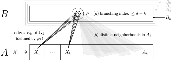
Figure 2: Illustration of central definitions in Lemma 11

Lemma 11.

Fix $d\in\mathbb{N}$. For every $0\leqslant k\leqslant d$ there is a formula $\varphi_{k}(x,y)$ in the signature consisting of a binary relation symbol $E$ and unary relation symbols $A,B,X_{0},\ldots,X_{k},B_{0},\ldots,B_{k}$, such that the following holds. Given a bipartite graph $G=(A,B,E)$ with $n\coloneqq|A|\geqslant 2$ such that no two vertices of $B$ have equal neighborhoods and $\mathrm{br}_{G}(B)\leqslant d$, there exist sets $B=B_{0}\supseteq\ldots\supseteq B_{k}$, pairwise disjoint sets $X_{0},\ldots,X_{k}\subseteq A$, and a bipartite graph $G_{k}=(A,B,E_{k})$ such that:

1. $|B_{k}|\geqslant\frac{|B|}{(300\ln n)^{k}}$;

2. $E_{k}$ is the set of pairs $ab$ such that $a\in A,b\in B$ and $(G,A,B,X_{0},\ldots,X_{k},B_{0},\ldots,B_{k})\models\varphi_{k}(a,b)$;

3. every $b\in B_{k}$ has at most $k$ neighbors in $X_{0}\cup\cdots\cup X_{k}$ in the graph $G_{k}$; and

4. for every $P\subseteq B_{k}$ such that all $b\in P$ have the same neighborhood in $X_{0}\cup\cdots\cup X_{k}$ in the graph $G_{k}$,

   1. $\mathrm{br}_{G_{k}}(P)\leqslant d-k$, and

   2. no two distinct vertices in $P$ have equal neighborhoods in $A-(X_{0}\cup\cdots\cup X_{k})$ in the graph $G_{k}$.

Proof.

We proceed by induction on $k$. For $k=0$ the formula $\varphi_{0}(x,y)\coloneqq E(x,y)$ satisfies the required conditions. Namely, for a given graph $G=(A,B,E)$ we define $B_{0}\coloneqq B$, $G_{0}\coloneqq G$, $X_{0}\coloneqq\varnothing$, and the required conditions trivially hold.

Assuming the statement holds for some value $k\geqslant 0$, we prove it for $k+1\leqslant d$. Let $\varphi_{k}(x,y)$ be as in the statement. Consider a bipartite graph $G=(A,B,E)$ and let $B=B_{0}\supseteq\ldots\supseteq B_{k}$, $X_{0},\ldots,X_{k}\subseteq A$, and $G_{k}$ be given by the induction assumption. Denote $A_{k}\coloneqq A-(X_{0}\cup\cdots\cup X_{k})$.

By a $k$-class we mean an inclusion-wise maximal set $P\subseteq B_{k}$ of vertices in $b\in B_{k}$ which have equal neighborhoods in $X_{0}\cup\cdots\cup X_{k}$ in the graph $G_{k}$. By assumption, $\mathrm{br}_{G_{k}}(P)\leqslant d-k$ for every $k$-class $P$. Therefore, for every vertex $a\in A$ and $k$-class $P$, we have

$$\min\left(\mathrm{br}_{G_{k}}(N_{G_{k}}(a)\cap P),\mathrm{br}_{G_{k}}(\overline{N}_{G_{k}}(a)\cap P)\right)<d-k.$$ (1)

Define a relation $E_{0}\subseteq A_{k}\times B_{k}\subseteq A\times B$ as

$$E_{0} \coloneqq \bigcup\,\bigl{\{}\{a\}\times P\bigm{|}a\in A_{k},\text{$P$ is a $k$-class with $\mathrm{br}_{G_{k}}(N_{G_{k}}(a)\cap P)=d-k$}\bigr{\}}$$

$$= \bigl{\{}ab\bigm{|}a\in A_{k}\textrm{ and }b\in P\text{ for some $k$-class $P$ with $\mathrm{br}_{G_{k}}(N_{G_{k}}(a)\cap P)=d-k$}\bigl{\}}.$$

Let $G_{k+1}\coloneqq(A,B,E(G_{k})\operatorname{\triangle}E_{0})$, where $\operatorname{\triangle}$ denotes the symmetric difference. So for a pair $ab$ with $a\in A$ and $b\in B$, we have that $ab\in E(G_{k+1})$ if and only if $ab$ belongs to exactly one of the sets $E(G_{k})$ and $E_{0}$. The relation $E_{k+1}$ is definable by a first-order formula, as stated in the next claim.

Claim 1.

There is a first-order formula $\varphi_{k+1}(x,y)$ over the signature $\{E,A,B,X_{0},\ldots,X_{k},B_{0},\ldots,B_{k}\}$, which is independent of $G$, such that for all $a\in A$ and $b\in B_{k}$ we have $(G,A,B,X_{0},\ldots,X_{k},B_{0},\ldots,B_{k})\models\varphi_{k+1}(a,b)$ if and only if ${ab\in E_{k+1}}$.

Proof.

Following the definition of the relation $E_{0}$, we construct a formula $\psi(x,y)$ defining the relation $E_{0}$, by combining the formula $\varphi_{k}$ obtained by the inductive assumption, and the formula $\beta_{d-k}$ obtained in Lemma 8. Then $\varphi_{k+1}(x,y)$ is defined as the XOR of the formulas $\psi$ and $\varphi_{k}$. We omit the easy details. ∎

Next, we note that the construction of $G_{k+1}$ from $G_{k}$ did not affect the neighborhoods in $X_{0}\cup\cdots\cup X_{k}$, nor the branching indices of subsets of $k$-classes.

Claim 2.

If $b\in B$, then the neighborhood of $b$ in $X_{0}\cup\cdots\cup X_{k}$ is the same when considered in $G_{k}$, and when considered in $G_{k+1}$.

Proof.

We have $E(G_{k+1})=E(G_{k})\operatorname{\triangle}E_{0}$, with $E_{0}\subseteq A_{k}\times B_{k}$ and $A_{k}$ disjoint from $X_{0}\cup\cdots\cup X_{k}$. ∎

Claim 3.

Let $P\subseteq B_{k}$ be a $k$-class and $Q\subseteq P$. Then $\mathrm{br}_{G_{k+1}}(Q)=\mathrm{br}_{G_{k}}(Q)$.

Proof.

We show that

$$\{N_{G_{k}}(a)\cap Q,\overline{N}_{G_{k}}(a)\cap Q\}=\{N_{G_{k+1}}(a)\cap Q,\overline{N}_{G_{k+1}}(a)\cap Q\}\qquad\textrm{for every }a\in A.$$ (2)

So, the two parts into which $a$ splits $Q$ are the same in $G_{k}$ as in $G_{k+1}$ (where the neighborhood is possibly swapped with the non-neighborhood). Claim 3 then follows from (2) by a straightforward induction.

Towards (2), fix $a\in A$. If $a\in X_{0}\cup\cdots\cup X_{k}$, the statement follows from Claim 2. Now, suppose $a\in A-(X_{0}\cup\cdots\cup X_{k})=A_{k}$. Then the set $\{a\}\times P$ is either disjoint from $E_{0}$, or is contained in $E_{0}$. In the first case, we have that $N_{G_{k}}(a)\cap P=N_{G_{k+1}}(a)\cap P$, while in the latter case, we have that $N_{G_{k}}(a)\cap P=\overline{N}_{G_{k+1}}(a)\cap P$. Either way, (2) follows. ∎

Let $B_{-}\subseteq B_{k}$ be the set of those vertices $b\in B_{k}$ such that $b$ has no neighbor in $A_{k}$ in the graph $G_{k+1}$, and let $B_{+}\coloneqq B_{k}-B_{-}$. We consider two cases, depending on which of the sets $B_{+},B_{-}$ is larger.

Case 1: $\boldsymbol{|B_{+}|\geqslant|B_{k}|/2}$.

Apply Lemma 10 to $G_{k+1}[A_{k},B_{+}]$, obtaining sets $B_{k+1}\subseteq B_{+}\subseteq B_{k}$ and $X_{k+1}\subseteq A_{k}$ such that $|B_{k+1}|\geqslant\frac{|B_{+}|}{150\ln n}\geqslant\frac{|B_{k}|}{300\ln n}$ and every vertex in $B_{k}$ has exactly one neighbor in $X_{k+1}$ in $G_{k+1}$. We check the required properties of $A_{k+1}$ and $B_{k+1}$. We have $|B_{k+1}|\geqslant\frac{|B_{k}|}{300\ln n}\geqslant\frac{|B|}{(300\ln n)^{k+1}}$ by the induction assumption, so condition (B.1) holds. Condition (B.2) holds by Claim 1.

To verify condition (B.3), let $b\in B_{k+1}$. We show that $b$ has at most $k+1$ neighbors in $X_{0}\cup\ldots,X_{k}\cup X_{k+1}$ in the graph $G_{k+1}$. By Claim 2, the adjacency between $b$ and $X_{0},\ldots,X_{k}$ in the graph $G_{k+1}$ is the same as in the graph $G_{k}$. Therefore, $b$ has at most $k$ neighbors in $X_{0}\cup\ldots\cup X_{k}$ in the graph $G_{k+1}$, as it does so in the graph $G_{k}$ by assumption. Furthermore, $b$ has exactly one neighbor in $X_{k+1}$ by construction. This verifies condition (B.3).

Finally, we verify condition (B.4). Let $P^{\prime}\subseteq B_{k+1}$ be a $(k+1)$-class. By Claim 2 and since every vertex in $B_{k+1}$ has exactly one neighbor in $X_{k+1}$, we can write $P^{\prime}=N_{G_{k+1}}(a_{0})\cap P\cap B_{k+1}$ for some $k$-class $P\subseteq B_{k}$ and some $a_{0}\in X_{k+1}$. We need to show that (a) $\mathrm{br}_{G_{k+1}}(P^{\prime})\leqslant d-k-1$, and that (b) $P^{\prime}$ does not contain distinct vertices with equal neighborhoods in $A_{k+1}$ in the graph $G_{k+1}$.

We first verify (a), that is, $\mathrm{br}_{G_{k+1}}(P^{\prime})<d-k$. For all $b\in P$ we have that $(a_{0},b)\in E_{0}$ if and only if $\mathrm{br}_{G_{k}}(N_{G_{k}}(a_{0})\cap P)=d-k$. Suppose first that

$$\mathrm{br}_{G_{k}}(N_{G_{k}}(a_{0})\cap P)<d-k.$$ (3)

Then $(a_{0},b)\notin E_{0}$ for all $b\in P$. As $E_{0}=E(G_{k})\operatorname{\triangle}E(G_{k+1})$, it follows that the neighborhood of $a_{0}$ in $P$ is the same when evaluated in $G_{k}$ and when evaluated in $G_{k+1}$. Therefore,

$$N_{G_{k}}(a_{0})\cap P\cap B_{k+1}=N_{G_{k+1}}(a_{0})\cap P\cap B_{k+1}=P^{\prime}.$$

In particular $P^{\prime}\subseteq N_{G_{k}}(a_{0})\cap P$, so $\mathrm{br}_{G_{k}}(P^{\prime})<d-k$ by (3) and the monotonicity of the branching index. Then also $\mathrm{br}_{G_{k+1}}(P^{\prime})<d-k$ by Claim 3. This confirms (a) in the considered case. Now suppose that

$$\mathrm{br}_{G_{k}}(N_{G_{k}}(a_{0})\cap P)\geqslant d-k.$$ (4)

Then $\mathrm{br}_{G_{k}}(\overline{N}_{G_{k}}(a_{0})\cap P)<d-k$ holds by (1). Dually to the previous case, we have that $(a_{0},b)\in E_{0}$ for all $b\in P$. By a reasoning dual to the one above,

$$\overline{N}_{G_{k}}(a_{0})\cap P\cap B_{k+1}=N_{G_{k+1}}(a_{0})\cap P\cap B_{k+1}=P^{\prime}.$$

Again, we conclude that $\mathrm{br}_{G_{k+1}}(P^{\prime})<d-k$, confirming (a).

We now verify (b), that is, we show that $P^{\prime}$ does not contain any pair of distinct vertices with equal neighborhoods in $A_{k+1}$ in the graph $G_{k+1}$. Let $b,b^{\prime}\in P^{\prime}$ be distinct. Then $b,b^{\prime}\in P$, so by assumption, $b$ and $b^{\prime}$ have distinct neighborhoods in $A_{k}$ in the graph $G_{k}$. Let $a\in A_{k}$ be such that

$$(a,b)\in E(G_{k})\Leftrightarrow(a,b^{\prime})\notin E(G_{k}).$$

Since $b,b^{\prime}\in P$ it follows that

$$(a,b)\in E_{0}\Leftrightarrow(a,b^{\prime})\in E_{0}.$$

As $E(G_{k+1})=E(G_{k})\operatorname{\triangle}E_{0}$, it follows that $(a,b)\in E(G_{k+1})\Leftrightarrow(a,b^{\prime})\notin E(G_{k+1})$. Since $a_{0}$ is the unique neighbor of both $b$ and $b^{\prime}$ in $X_{k+1}$ in the graph $G_{k+1}$, and $a$ is adjacent in $G_{k+1}$ either to $b$ or $b^{\prime}$, we conclude $a\not\in X_{k+1}$. Therefore, $a$ witnesses that $b$ and $b^{\prime}$ have distinct neighborhoods in $A_{k+1}=A_{k}-X_{k+1}$ in the graph $G_{k+1}$.

Thus, we verified condition (B.4), and completed Case 1.

Case 2: $\boldsymbol{|B_{-}|>|B_{k}|/2}$.

Let $B_{k+1}\coloneqq B_{-}\subseteq B_{k}$ consist of the vertices with no neighbors in $A_{k}$ in the graph $G_{k+1}$. Set $X_{k+1}\coloneqq\varnothing$. We verify the required conditions for this choice of $B_{k+1}$ and $X_{k+1}$.

Condition (B.1) holds as $|B_{k+1}|\geqslant|B_{k}|/2\geqslant\frac{|B|}{2\cdot(300\ln n)^{k}}\geqslant\frac{|B|}{(300\ln n)^{k+1}}$, condition (B.2) holds by Claim 1, and condition (B.3) holds by Claim 2. To prove condition (B.4), we show the following

Claim 4.

No two distinct vertices of $B_{k+1}$ have equal neighborhoods in $X_{0}\cup\cdots\cup X_{k}$ in $G_{k+1}$.

Proof.

Suppose that distinct $b,b^{\prime}\in B_{k+1}$ have equal neighborhoods in $X_{0}\cup\cdots\cup X_{k}$ in $G_{k+1}$. Using Claim 2, let $P$ be the $k$-class such that $b,b^{\prime}\in P$. By condition (B.4),(B.4)(b), we have that $b$ and $b^{\prime}$ have different neighborhoods in $A_{k}$ in $G_{k}$. Let $a\in A_{k}$ be adjacent to exactly one of $b,b^{\prime}$ in $G_{k}$. As $b$ and $b^{\prime}$ belong to the same $k$-class $P$, it follows by definition of $E_{0}$ that $ab\in E_{0}\Leftrightarrow ab^{\prime}\in E_{0}$. As $E(G_{k})=E(G_{k+1})\operatorname{\triangle}E_{0}$, we observe that $a$ is adjacent to exactly one of $b,b^{\prime}$ in $G_{k+1}$. Moreover, as $b,b^{\prime}\in B_{-}$, and vertices in $B_{-}$ have no neighbors in $A_{k}$ in the graph $G_{k}$, it follows that $a\notin A_{k}$, so $a\in X_{0}\cup\cdots\cup X_{k}$. Therefore, $b$ and $b^{\prime}$ have distinct neighborhoods in $X_{0}\cup\cdots\cup X_{k}$ in $G_{k+1}$, a contradiction which completes the proof. ∎

As $X_{0}\cup\cdots\cup X_{k}=X_{0}\cup\cdots\cup X_{k+1}$, condition (B.4) follows trivially from Claim 4. This completes Case 2, and the proof of the lemma. ∎

Next, we proceed to Proposition 9, which is obtained by setting $k=d$ in Lemma 11 and studying the consequences of condition (B.4) in this case. We repeat the statement. See 9

Proof.

Apply Lemma 11 to $k=d$, obtaining a formula $\varphi_{d}(x,y)$ involving the edge relation $E$ and some unary predicates. Let $\mathsf{T}_{d}$ be the transduction that first assigns these unary predicates, then applies $\varphi_{d}(x,y)$, and finally takes an arbitrary subgraph. Given a bipartite graph $G=(A,B,E)$, let $B_{0},\ldots,B_{d},X_{0},\ldots,X_{d}$ and $G_{d}=(A,B,E^{\prime})$ be as in the statement of Lemma 11. Set $A^{\prime}\coloneqq X_{0}\cup\cdots\cup X_{d}$, $B^{\prime}\coloneqq B_{d}$. Let $G^{\prime}\coloneqq G_{d}[A^{\prime},B^{\prime}]$ be the bipartite graph induced on $A^{\prime}$ and $B^{\prime}$. Then $G^{\prime}\in\mathsf{T}_{d}(G)$.

Conditions (A.1) and (A.2) follow immediately from the appropriate conditions in Lemma 11. We verify condition (A.3). Suppose $b,b^{\prime}\in B^{\prime}$ have equal neighborhoods in $A^{\prime}$ in the graph $G^{\prime}$. By condition (B.4),(B.4)(a) in Lemma 11 applied to $P=\{b,b^{\prime}\}$, we have that $\mathrm{br}_{G_{d}}(P)=0$. Hence, $b$ and $b^{\prime}$ have equal neighborhoods in $G_{d}$. By condition (B.4),(B.4)(b), we get $b=b^{\prime}$. This completes the proof of Proposition 9. ∎

The next lemma combines Proposition 9 with Theorem 5 and Theorem 6.

Lemma 12.

Let $\mathscr{C}$ be a monadically stable class of bipartite graphs such that for all $G=(A,B,E)\in\mathscr{C}$ no vertices in $B$ have equal neighborhoods and let $\varepsilon>0$. Then for every $(A,B,E)\in\mathscr{C}$ we have that $|B|\leqslant\mathcal{O}_{\mathscr{C},d,\varepsilon}(|A|^{1+\varepsilon})$.

Proof.

Let $d$ be as in Theorem 7, so that $\mathrm{br}_{G}(B)\leqslant d$ for all $G=(A,B,E)\in\mathscr{C}$. Let $\mathsf{T}_{d}$ be as in Proposition 9. Without loss of generality, we may assume $|A|\geqslant 2$ for all $(A,B,E)\in\mathscr{C}$. We associate with every $G\in\mathscr{C}$ a bipartite graph $F(G)\in\mathsf{T}_{d}(G)$ satisfying the conditions listed in Proposition 9. Let $\mathscr{D}=\{F(G)\colon G\in\mathscr{C}\}$. Then $\mathscr{D}$ is monadically stable, as $\mathscr{D}\subseteq\mathsf{T}_{d}(\mathscr{C})$ and $\mathscr{C}$ is monadically stable. Moreover, the class $\mathscr{D}$ avoids $K_{d+1,d+1}$ as a subgraph, by condition (A.2). Therefore, Theorem 6 implies that $\mathscr{D}$ is nowhere dense. By (A.3), for every graph $(A^{\prime},B^{\prime},E^{\prime})\in\mathscr{D}$, there is no pair of vertices in $B^{\prime}$ with equal neighborhoods in $A^{\prime}$. Consider $G=(A,B,E)\in\mathscr{C}$ and $F(G)=(A^{\prime},B^{\prime},E^{\prime})\in\mathscr{D}$. By Theorem 5 we have for $\delta\coloneqq\varepsilon/2$ that

$$|B^{\prime}|\leqslant\mathcal{O}_{\mathscr{D},\delta}\left(|A^{\prime}|^{1+\delta}\right).$$

On the other hand, by condition (A.1) we infer that

$$|B^{\prime}|\geqslant|B|/(300\ln|A|)^{d}.$$

As $|A^{\prime}|\leqslant|A|$, we obtain

$$|B|\leqslant|B^{\prime}|\cdot(300\ln|A|)^{d}\leqslant(300\ln|A|)^{d}\cdot\mathcal{O}_{\mathscr{D},\delta}\left(|A|^{1+\delta}\right)\leqslant\mathcal{O}_{\mathscr{C},d,\varepsilon}\left(|A|^{1+\varepsilon}\right).\qed$$

Theorem 3, restated for convenience, now follows easily.

See 3

Proof.

For a graph $G=(V,E)$, let $B(G)$ denote the bipartite graph with sides $V\times\{1\}$ and $V\times\{2\}$, and edges $(u,1),(v,2)$ for all $u,v$ such that $u=v$ or $uv\in E$. Let $\mathscr{B}$ be the class of all induced subgraphs of graphs $B(G)$, for $G\in\mathscr{C}$. Then $\mathscr{B}$ monadically stable. One way to argue this is that $\mathscr{B}$ is obtained from $\mathscr{C}$ by a transduction with copying, and it is known that such transductions preserve monadic stability. It is alternatively not difficult to prove directly that if $\mathscr{D}$ transduces the class of all half-graphs, then so does $\mathscr{C}$. By Lemma 12, for all $(A,B,E)\in\mathscr{B}$ such that no two vertices in $B$ have equal neighborhoods,

$$|B|\leqslant\mathcal{O}_{\mathscr{C},\varepsilon}\left(|A|^{1+\varepsilon}\right).$$

Let $G\in\mathscr{C}$ and $A\subseteq V(G)$. Choose $B\subseteq V$ such that $N[v]\cap A\neq N[v^{\prime}]\cap A$ for all $v,v^{\prime}\in B$. Then $|\{N[v]\cap A\colon v\in V(G)\}|=|B|$. As $(A,B,\{ab\colon a\in A,b\in B,a\in N[b]\})\in\mathscr{B}$, and no two vertices in $B$ have equal neighborhoods in this graph, we conclude that

$$|\{N[v]\cap A\colon v\in V(G)\}|=|B|\leqslant\mathcal{O}_{\mathscr{C},\varepsilon}\left(|A|^{1+\varepsilon}\right).\qed$$

3.2 Sparse neighborhood covers

For a graph $G$ and vertex subset $X$, the weak diameter of $X$ in $G$ is the maximum distance in $G$ between members of $X$: $\mathrm{diam}_{G}(X)\coloneqq\max_{u,v\in X}\mathrm{dist}_{G}(u,v)$. As discussed in Section 1, the following notion of a neighborhood cover is of key importance to us.

Definition 5.

Let $G$ be a graph and $r$ be a positive integer. A family $\mathcal{K}$ of subsets of vertices of $G$ is called a distance-$r$ neighborhood cover of $G$ if for every vertex $u$ of $G$ there exists $C\in\mathcal{K}$ such that $\mathrm{Ball}_{r}[u]\subseteq C$. The diameter of $\mathcal{K}$ is the maximum weak diameter among the sets of $\mathcal{K}$, while the overlap of $\mathcal{K}$ is the maximum number of sets of $\mathcal{K}$ that intersect at a single vertex:

$$\mathrm{diam}(\mathcal{K})\coloneqq\max_{C\in\mathcal{K}}\ \mathrm{diam}_{G}(C)\qquad\textrm{and}\qquad\mathrm{overlap}(\mathcal{K})\coloneqq\max_{u\in V(G)}|\{C\in\mathcal{K}~{}|~{}u\in C\}|.$$

Elements of a neighborhood cover $\mathcal{K}$ will often be called clusters.

The results of Dreier, Mählmann, and Siebertz [DMS23] require the construction of distance-$r$ neighborhood covers with small overlap, for all $r\in\mathbb{N}$. We now explain how such covers can be obtained by finding distance-$1$ covers in interpretations of the given graph.

For a graph $G$, let the $r$th power of $G$, denoted $G^{r}$, be the graph on the same vertex set as $G$ where vertices $u,v$ are adjacent if and only if the distance between $u$ and $v$ in $G$ is at most $r$. Note that for every fixed $r$, $G^{r}$ can be easily interpreted in $G$ using a formula that checks whether the distance between $u$ and $v$ is at most $r$. The next lemma shows that finding a distance-$1$ neighborhood cover in $G^{r}$ immediately yields a distance-$r$ neighborhood cover in $G$ with the same overlap.

Lemma 13.

Let $G$ be a graph, $r$ be a positive integer, and $\mathcal{K}$ be a distance-$1$ neighborhood cover of $G^{r}$ of diameter $d$. Then $\mathcal{K}$ is also a distance-$r$ neighborhood cover of $G$ of diameter at most $dr$.

Proof.

That $\mathcal{K}$ is a distance-$r$ neighborhood cover of $G$ follows immediately from the observation that for every vertex $u$, $\mathrm{Ball}^{G^{r}}_{1}[u]=\mathrm{Ball}^{G}_{r}[u]$. That the weak diameter of $\mathcal{K}$ is at most $dr$ follows immediately from triangle inequality and the definition of the graph $G^{r}$. ∎

In this section we provide a construction of neighborhood covers with small overlap for monadically stable graph classes. Formally, we prove the following result.

Theorem 14.

Let $\mathscr{C}$ be a monadically stable class of graphs. Then for every $r\in\mathbb{N}$ and $n$-vertex graph $G\in\mathscr{C}$ there exists a distance-$r$ neighborhood cover of $G$ with diameter at most $4r$ and whose overlap can be bounded by $\mathcal{O}_{\mathscr{C},r,\varepsilon}(n^{\varepsilon})$ for every $\varepsilon>0$. Moreover, there is an algorithm that computes such a neighborhood cover in time complexity that can be bounded by $\mathcal{O}_{\mathscr{C},r,\varepsilon}(n^{4+\varepsilon})$, for every $\varepsilon>0$.

We note that the algorithm of Theorem 14 actually does not depend on the class $\mathscr{C}$ or the value of $\varepsilon$: it is a single algorithm that, when supplied with a graph $G\in\mathscr{C}$, will always output a neighborhood cover of $G$ with diameter and overlap bounded as asserted.

The main ingredient towards proving Theorem 14 will be a tool introduced by Welzl [Wel88] in the context of geometric range queries, called spanning paths with low crossing number, which we will call Welzl orders. To introduce them, we need some definitions. We remark that for convenience, our terminology slightly differs from that of Welzl.

Consider a set system $\mathcal{S}=(U,\mathcal{F})$, where $U$ is a finite universe and $\mathcal{F}$ is a family of subsets of $\mathcal{F}$. The growth function of $\mathcal{S}$ is the function $\pi_{\mathcal{S}}(\cdot)$ that assigns each positive integer $n$ the value

$$\pi_{\mathcal{S}}(n)\coloneqq\max_{A\subseteq U,|A|\leqslant n}\ |\{X\cap A\colon X\in\mathcal{F}\}|.$$

In other words, $\pi_{\mathcal{S}}(n)$ is the largest number of traces that the sets from $\mathcal{F}$ leave on a subset $A\subseteq U$ of size $n$, where the trace left by $X\in\mathcal{F}$ on $A$ is $X\cap A$. For example, the Sauer-Shelah Lemma states that if the VC dimension of $\mathcal{S}$ is $d$, then $\pi_{\mathcal{S}}(n)\leqslant\mathcal{O}(n^{d})$. On the other hand, from Theorem 3 we immediately obtain the following.

Corollary 15.

Let $\mathscr{C}$ be a monadically stable class of graphs and $\mathscr{D}$ be the class of set systems of closed neighborhoods of graphs in $\mathscr{C}$, that is,

$$\mathscr{D}\coloneqq\bigl{\{}\bigl{(}V(G),\{N_{G}[u]\colon u\in V(G)\}\bigr{)}\colon G\in\mathscr{C}\bigr{\}}.$$

Then for every $\mathcal{S}\in\mathscr{D}$, we have $\pi_{\mathcal{S}}(n)\leqslant\mathcal{O}_{\mathscr{C},\varepsilon}(n^{1+\varepsilon})$ for all $\varepsilon>0$.

Next, for a set system $\mathcal{S}=(U,\mathcal{F})$ and a total order $\preccurlyeq$ on $U$, we define the crossing number of $\preccurlyeq$ as follows. For $X\in\mathcal{F}$, the crossing number of $X$ with respect to $\preccurlyeq$ is the number of pairs $(u,u^{\prime})$ of elements of $U$ such that

• $u^{\prime}$ is the immediate successor of $u$ in $\preccurlyeq$, and

• exactly one of $u$ and $u^{\prime}$ belongs to $X$.

Note that this is equivalent to the following: the crossing number of $X$ is the least $k$ such that $\preccurlyeq$ can be partitioned into $k+1$ intervals so that every interval is either contained in or disjoint from $X$. Then the crossing number of $\preccurlyeq$ is the maximum crossing number of any $X\in\mathcal{F}$ with respect to $\preccurlyeq$.

The following statement is the main result of [Wel88].

Theorem 16 (Theorem 4.2 and Lemma 3.3 of [Wel88], see also Theorem 4.3 of [CW89]).

Suppose $\mathcal{S}=(U,\mathcal{F})$ is a set system with $\pi_{\mathcal{S}}(n)\leqslant\mathcal{O}(n^{d})$, where $d>1$ is a real. Then there exists a total order $\preccurlyeq$ on $U$ with crossing number bounded by $\mathcal{O}(|U|^{1-1/d}\cdot\log|U|)$. Moreover, there is an algorithm that, given $\mathcal{S}$, computes such an order in time $\mathcal{O}(\pi_{\mathcal{S}}(|U|)\cdot(|U|+|\mathcal{F}|)^{3})$.

For the algorithmic statement, see the remark provided below the proof of [Wel88, Theorem 4.2]. Also, we note that the algorithm of Theorem 16 does not need to be supplied with the value of $d$: it is a single algorithm that, given $\mathcal{S}$, computes a total order $\preccurlyeq$, and the guarantee on the crossing number of $\preccurlyeq$ follows from the assumption on the growth function of $\mathcal{S}$.

Next, we show that, given a total order with a low crossing number, we can construct a neighborhood cover with a small overlap and constant diameter using a relatively easy greedy construction.

Lemma 17.

Suppose $G=(V,E)$ is a graph, $\mathcal{S}\coloneqq(V,\{N[u]\colon u\in V\})$ is the set system of closed neighborhoods in $G$, and $\preccurlyeq$ is a total order on $V$ with crossing number $k$ (with respect to $\mathcal{S}$). Then $G$ admits a distance-$1$ neighborhood cover with diameter at most $4$ and overlap at most $k+1$, and such a neighborhood cover can be computed, given $G$ and $\preccurlyeq$, in time $\mathcal{O}(|V|^{3})$.

Proof.

We need some auxiliary definitions about the order $\preccurlyeq$. An interval is a set $I\subseteq V$ that is convex in $\preccurlyeq$: $u\preccurlyeq v\preccurlyeq w$ and $u,w\in I$ entails $v\in I$. A prefix of an interval $I$ is an interval $J$ such that $u,v\in I$, $u\preccurlyeq v$ and $v\in J$ entails $u\in J$. An interval $I$ is compact if $I\subseteq N[u]$ for some $u\in V$. We perform the following greedy construction of a partition $\mathcal{I}$ of $V$ into intervals:

• Start with $\mathcal{I}\coloneqq\varnothing$.

• As long as $V-\bigcup\mathcal{I}\neq\varnothing$, let $I$ be the largest prefix of $V-\bigcup\mathcal{I}$ that is compact. Then add $I$ to $\mathcal{I}$.

Thus, $\mathcal{I}$ consists of compact nonempty intervals. A straightforward implementation of the procedure presented above computes $\mathcal{I}$ in time $\mathcal{O}(|V|^{3})$.

We claim that $\mathcal{K}\coloneqq\{N[I]\colon I\in\mathcal{I}\}$ is a neighborhood cover of $G$ of diameter at most $4$ and overlap at most $k+1$. That $\mathcal{K}$ is a neighborhood cover is clear: if $u$ is a vertex and $I\in\mathcal{I}$ is such that $u\in I$, then $N[u]\subseteq N[I]$. Also observe that the compactness of every $I\in\mathcal{I}$ implies that $N[I]$ has weak diameter at most $4$. We are left with proving the claimed bound on the overlap.

Fix any vertex $v\in V$. Call a vertex $u\in V$ a crossing for $v$ if $u$ has a successor $u^{\prime}$ in $\preccurlyeq$ and $N[v]$ contains exactly one of the vertices $u$ and $u^{\prime}$. Since $\mathcal{S}$ has crossing number $k$, there are at most $k$ distinct crossings for $v$. We claim the following:

for every interval $I\in\mathcal{I}$ such that $v\in N[I]$,

$I$ contains a crossing for $v$ or $I$ contains the $\preccurlyeq$-largest element of $V$.

Since there can be at most $k$ crossings for $v$ and at most one interval can contain the $\preccurlyeq$-largest element, this claim will conclude the proof: it implies that $v$ belongs to at most $k+1$ clusters of $\mathcal{K}$.

To show the claim, first note that $v\in N[I]$ implies that $I\cap N[v]\neq\varnothing$. If also $I-N[v]\neq\varnothing$ then clearly $I$ contains a crossing for $v$, so assume otherwise: $I\subseteq N[v]$. Let $u$ be the largest element of $I$ in the $\preccurlyeq$ order. Unless $u$ is actually the $\preccurlyeq$-largest element of $V$, $u$ has a successor $u^{\prime}$ and $u^{\prime}\in I^{\prime}\in\mathcal{I}$ for some $I^{\prime}\neq I$. Also, unless $u$ itself is a crossing for $v$, we have $u^{\prime}\in N[v]$. We now observe that $I\cup\{u^{\prime}\}$ is an interval that is compact, as witnessed by the vertex $v$, and is strictly larger than $I$. This contradicts the construction of $\mathcal{I}$: in the round when $I$ was added to $\mathcal{I}$, we could have added the larger interval $I\cup\{u^{\prime}\}$ instead. This concludes the proof of the claim and of the lemma. ∎

We may now combine all the gathered tools and prove Theorem 14.

Proof of Theorem 14.

Let $G\in\mathscr{C}$ be the input graph. By Lemma 13, it suffices to compute a distance-$1$ neighborhood cover with diameter $4$ for the $r$th power $G^{r}=(V,E)\in\mathscr{C}^{r}$ of $G$, where $\mathscr{C}^{r}$ is the class that contains the $r$th power of every graph in $\mathscr{C}$. As $\mathscr{C}$ interprets $\mathscr{C}^{r}$, the latter class is still monadically stable. Let $\mathcal{S}\coloneqq(V,\{N[u]\colon u\in V\})$ be the set system of closed neighborhoods in $G^{r}$. By Corollary 15, we have $\pi_{\mathcal{S}}(n)\leqslant\mathcal{O}_{\mathscr{C},r,\varepsilon}(n^{1+\varepsilon})$ for every $\varepsilon>0$. Apply the algorithm of Theorem 16 to $\mathcal{S}$, to obtain a total order $\preccurlyeq$ on $V$ such that the crossing number of $\preccurlyeq$ is bounded by $\mathcal{O}_{\mathscr{C},r,\varepsilon}(|V|^{1-\frac{1}{1+\varepsilon}}\cdot\log|V|)\leqslant\mathcal{O}_{\mathscr{C},r,\varepsilon}(|V|^{\varepsilon})$ for every $\varepsilon>0$. By Theorem 16, this application takes time $\mathcal{O}_{\mathscr{C},r,\varepsilon}(|V|^{4+\varepsilon})$. It now suffices to apply the algorithm of Lemma 17 to $G^{r}$ and $\preccurlyeq$. ∎

We remark that the construction presented above actually provides a neighborhood cover with far stronger structural properties than just a subpolynomial bound on the overlap. Namely, if we define the incidence graph of a neighborhood cover to be the bipartite graph with vertices on one side, clusters on the other side, and adjacency defined through membership (of a vertex to a cluster), then the incidence graphs of the constructed neighborhood covers form a class that is almost nowhere dense, in the sense that edge density in shallow minors is bounded subpolynomially in the vertex count. We view this as a first step towards a proof of a relaxed variant of the so-called Sparsification Conjecture [Oss21], which postulates that every monadically stable class of graphs can be transduced from a nowhere dense class. The formal statement of this result together with the relevant discussion can be found in Appendix C.

3.3 Model checking

The full version of [DMS23] defines the notion of flip-closed sparse neighborhood covers ([DMS23, Definition 3]), and shows that one can solve the model checking problem in time $f(\|\varphi\|)\cdot n^{11}$ on every monadically stable graph class $\mathscr{C}$ admitting such neighborhood covers ([DMS23, Theorem 5]). Here, flip-closed means that for every fixed $k\in\mathbb{N}$, the class $\mathscr{C}_{k}$ of all $k$-flips of graphs from $\mathscr{C}$ still admits sparse neighborhood covers (more precisely, distance-$r$ neighborhood covers of diameter $\mathcal{O}_{\mathscr{C},r}(1)$ and overlap $\mathcal{O}_{\mathscr{C},r,\varepsilon}(n^{\varepsilon})$, for any $\varepsilon>0$ and $r\in\mathbb{N}$). Since $\mathscr{C}_{k}$ is monadically stable provided $\mathscr{C}$ is, our Theorem 14 implies in particular that every monadically stable class admits flip-closed sparse neighborhood covers, and thus immediately yields, in combination with [DMS23], an fpt model checking algorithm for monadically stable classes.

However, in [DMS23, Theorem 10], neighborhood covers were approximated using an LP-based rounding technique in time $\mathcal{O}(n^{9.8})$, while our algorithm of Theorem 14 runs in time $\mathcal{O}_{\mathscr{C},r,\varepsilon}(n^{4+\varepsilon})$. In Appendix B, we argue that substituting the neighborhood cover subroutine from [DMS23] with ours yields the faster running time promised in Theorem 1, restated below.

See 1

4 Hardness results for unstable classes

In this section we characterize monadically stable graph classes in terms of forbidden induced subgraphs and subsequently derive algorithmic hardness results. Before diving into the details, we will first give an overview of the proof strategy. The starting point to our characterization is the work of Gajarský et al. [GMM⁺23] which gives a particular yet irregular obstructions to monadic stability (Figure 3). We regularize these obstructions via different Ramsey-type theorems. Intuitively, we argue that within a large enough irregular obstruction, we may find a smaller obstruction which is regular, in the sense that adjacency within it depends on certain appropriately chosen color classes. Moreover, edge-stability ensures that the relationship between these color classes is “orderless”, thus further simplifying the structure of these obstructions and obtaining the concrete patterns of Theorem 4 below.

See 4

The contribution of this characterization is twofold: not only it gives rise to a more natural definition of monadic stability akin to the usual definition of nowhere density, but moreover, the obtained patterns that avoid half-graphs may be shown to effectively interpret the class of all graphs via existential formulas; this essentially yields Theorem 2.

See 2

We briefly discuss our approach to the above. By Theorem 4 and hereditariness, it suffices to consider two cases: $\mathscr{C}$ either contains a $k$-flip of every $r$-subdivided clique or a $k$-flip of every $r$-web, for some fixed $k,r\geqslant 2$. The two cases differ in their technical details; nonetheless, the general proof strategy is the same for both, and so we only highlight the case of subdivided cliques. Up to increasing the value of $r$ by a constant factor, we may ensure by hereditariness that $\mathscr{C}$ also contains a $k$-flip of every $r$-subdivided biclique: an $r$-subdivision of a complete bipartite graph. While a simple graph gadget argument reveals that every class that contains all non-flipped $r$-subdivided bicliques existentially interprets the class of all graphs, we only know that $\mathscr{C}$ contains $k$-flip of those. The main challenge therefore lies in definably “reversing” the flips. Using Ramsey’s theorem for bipartite graphs, the pigeonhole principle, and hereditariness, we conclude that $\mathscr{C}$ contains for each $r$-subdivided biclique a $k$-flip that is in a certain sense canonical. Moreover, for each canonical flip, the flip partition $\mathcal{P}$ is minimal in the sense that no two parts can be merged. Given a canonical $k$-flip of an $r$-subdivided biclique, the key to reversing the flip is to recover for every vertex $v$ its part $\mathcal{P}(v)$ in $\mathcal{P}$. From here, a rather naive strategy proceeds by existentially quantifying a representative vertex $z_{i}$ for each part $P_{i}\in\mathcal{P}$, checking the adjacency between $v$ and a realization to $z_{i}$ to see whether $\mathcal{P}(v)$ was flipped with $P_{i}$, and finally determining $\mathcal{P}(v)$ using minimality of the flip partition. However, this approach runs into problems as the realization of each quantified vertex $z_{i}$ does not necessarily lie within $P_{i}$. To overcome this, we instead quantify a small set $Z_{i}$ of representatives for each part, and check whether $v$ is connected to the majority of $Z_{i}$. Using the structural properties of subdivided bicliques, we then argue that this allows us to approximately recover $\mathcal{P}(v)$, up to parts that behave symmetrically. This is sufficient to definably tell which pairs of vertices were flipped.

This provides us with a way to recover the unflipped edge relation of a subdivided clique within its $k$-flip. Building up from the edge formula, we obtain for every existential formula $\varphi$ an existential formula $\mathrm{flip}(\varphi)$ such that $\varphi$ is true in a subdivided clique if and only if $\mathrm{flip}(\varphi)$ is true in its $k$-flip present in $\mathscr{C}$.

4.1 Auxiliary Ramsey-type results

Since variants of Ramsey’s Theorem are at the core of our proofs, we begin by providing a brief overview of these. Here are the two standard formulations: the classic one and the one tailored to bipartite graphs. By the biclique of order $n$ we mean $K_{n,n}$.

Lemma 18 (Ramsey’s Theorem for Cliques).

There exists a computable function $\mathcal{R}\colon\mathbb{N}\times\mathbb{N}\to\mathbb{N}$ such that for every $k,n\in\mathbb{N}$ and every edge-coloring of the clique of size $\mathcal{R}(k,n)$ with $k$ colors we may find a sub-clique of size $n$ which is monochromatic with respect to this coloring.

Lemma 19 (Ramsey’s Theorem for Bicliques).

There exists a computable function $\mathcal{R}_{\mathrm{bip}}\colon\mathbb{N}\times\mathbb{N}\to\mathbb{N}$ such that for every $k,n\in\mathbb{N}$ and every edge-coloring of the biclique of order $\mathcal{R}_{\mathrm{bip}}(k,n)$ with $k$ colors, we may find a sub-biclique of order $n$ which is monochromatic with respect to this coloring.

We will also use a generalization of Ramsey’s Theorem where instead of $2$-element subsets, one colors (ordered) $\ell$-tuples of elements. To introduce this variant, we need some notation.

For a pair $(a,b)$ of elements of a linearly ordered set $(A,\leqslant)$, let $\mathrm{otp}(a,b)\in\{<,=,>\}$ indicate whether $a<b$, $a=b$, or $a>b$ holds. For $\ell\geqslant 1$ and an $\ell$-tuple of elements $a_{1},\ldots,a_{\ell}$ of a linearly ordered set $(A,\leqslant)$, define the order type of $(a_{1},\ldots,a_{\ell})$, denoted $\mathrm{otp}(a_{1},\ldots,a_{\ell})$, as the tuple $(\mathrm{otp}(a_{i},a_{j}))_{1\leqslant i<j\leqslant\ell}$.

With this notation in place, we can state the general form of Ramsey’s Theorem that we will use. It follows easily from the standard formulation of Ramsey’s Theorem for colorings of $\ell$-element subsets of an $n$-element set using $k$ colors (generalizing the case $\ell=2$ corresponding to colorings of cliques considered above).

Lemma 20 (General Ramsey’s Theorem).

Fix $k,\ell,n\in\mathbb{N}$. Then there is some $N\in\mathbb{N}$ such that for every coloring

$$\lambda\colon[N]^{\ell}\to[k]$$

there is a subset $I\subseteq[N]$ such that $|I|=n$ and for all $(a_{1},\ldots,a_{\ell})\in I^{\ell}$, we have that $\lambda(a_{1},\ldots,a_{\ell})$ depends only on $\mathrm{otp}(a_{1},\ldots,a_{\ell})$. That is, there is a function $f$ such that $\lambda(a_{1},\ldots,a_{\ell})=f(\mathrm{otp}(a_{1},\ldots,a_{\ell}))$, for all $(a_{1},\ldots,a_{\ell})\in I^{\ell}$.

From Lemma 20 we derive a variant of Ramsey’s Theorem for grids. For this, we again need some terminology.

Fix $n\in\mathbb{N}$. By an ordered $n$-grid we mean the relational structure $\mathbf{G}_{n}$ with domain $[n]\times[n]$ and two relations $\leqslant_{1},\leqslant_{2}$ satisfying:

$$(i,j)\leqslant_{1}(i^{\prime},j^{\prime})\iff i\leqslant i^{\prime};$$

$$(i,j)\leqslant_{2}(i^{\prime},j^{\prime})\iff j\leqslant j^{\prime}.$$

For compatibility with the graph notation, the domain of $\mathbf{G}_{n}$ will be denoted by $V(\mathbf{G}_{n})$. For $(a,b)=((a_{1},a_{2}),(b_{1},b_{2}))\in V(\mathbf{G}_{n})^{2}$, the atomic type of $(a,b)$ is defined as

$$\textnormal{atp}(a,b)\coloneqq(\mathrm{otp}(a_{1},b_{1}),\mathrm{otp}(a_{2},b_{2})).$$

In other words, $\textnormal{atp}(a,b)\in\{<,=,>\}^{2}$ encodes the relative order of $a$ and $b$ in $\leqslant_{1}$ and $\leqslant_{2}$.

A pair coloring of $\mathbf{G}_{n}$ is a map $\chi\colon V(\mathbf{G}_{n})^{2}\to[k]$, where $k\in\mathbb{N}$. We say that a pair coloring $\chi$ is homogeneous if for all $(a,b),(c,d)\in V(\mathbf{G}_{n})^{2}$, we have

$$\textnormal{atp}(a,b)=\textnormal{atp}(c,d)\implies\chi(a,b)=\chi(c,d).$$

In other words, the color of a pair $(a,b)$ depends only on $\textnormal{atp}(a,b)$.

Lemma 21 (Grid Ramsey Theorem).

There is a computable function $\mathcal{R}_{\mathrm{grid}}\colon\mathbb{N}\times\mathbb{N}\to\mathbb{N}$ such that for every $k,n\in\mathbb{N}$ and every pair coloring of the ordered $\mathcal{R}_{\mathrm{grid}}(k,n)$-grid with $k$ colors there is an induced copy of the ordered $n$-grid which is homogeneous with respect to this coloring.

Proof.

Fix $k,n\in\mathbb{N}$. Let $\mathcal{R}_{\mathrm{grid}}(k,n)\coloneqq N$ be the number obtained from Lemma 20 applied to the values $k$, $\ell=4$ and $2n$. Let $\mathbf{G}_{N}$ be the ordered $N$-grid, and let $\chi\colon V(\mathbf{G}_{N})^{2}\to[k]$ be a pair coloring of pairs in $\mathbf{G}_{N}$ using $k$ colors. Define a coloring $\lambda\colon[N]^{4}\to[k]$ by setting

$$\lambda(a_{1},a_{2},b_{1},b_{2})\coloneqq\chi((a_{1},a_{2}),(b_{1},b_{2}))\qquad\text{for $(a_{1},a_{2},b_{1},b_{2})\in[N]^{4}$.}$$

Thus, $\lambda$ defines a coloring of elements of $[N]^{4}$, using $k$ colors.

By Lemma 20, we can find a subset $I\subseteq[N]$ of size $2n$ such that the restriction of $\lambda$ to $I$ is homogeneous, that is, $\lambda(a_{1},a_{2},b_{1},b_{2})$ depends only on $\mathrm{otp}(a_{1},a_{2},b_{1},b_{2})$.

Let $I_{1}$ be the first $n$ elements of $I$ and $I_{2}$ be the last $n$ elements of $I$.

Consider the substructure $\mathbf{A}$ of $\mathbf{G}_{N}$ induced by pairs $(a_{1},a_{2})$ with $a_{1}\in I_{1}$ and $a_{2}\in I_{2}$. Clearly, $\mathbf{A}$ is isomorphic to $\mathbf{G}_{n}$. We show that the restriction of $\chi$ to $\mathbf{A}$ is homogeneous.

Note that for every tuple $((a_{1},a_{2}),(b_{1},b_{2}))\in(I_{1}\times I_{2})^{2}$, we have that

$$\mathrm{otp}(a_{1},a_{2})=\mathrm{otp}(b_{1},b_{2})=\mathrm{otp}(a_{1},b_{2})=\mathrm{otp}(b_{1},a_{2})={<},$$

since $a_{1},b_{1}\in I_{1}$ and $a_{2},b_{2}\in I_{2}$ and $x<y$ for all $x\in I_{1}$ and $y\in I_{2}$.

Let $((a_{1},a_{2}),(b_{1},b_{2}))\in(I_{1}\times I_{2})^{2}$ and $((a^{\prime}_{1},a^{\prime}_{2}),(b^{\prime}_{1},b^{\prime}_{2}))\in(I_{1}\times I_{2})^{2}$ be two pairs such that

$$\textnormal{atp}((a_{1},a_{2}),(b_{1},b_{2}))=\textnormal{atp}((a^{\prime}_{1},a^{\prime}_{2}),(b^{\prime}_{1},b^{\prime}_{2})).$$

This implies that $\mathrm{otp}(a_{1},b_{1})=\mathrm{otp}(a_{1}^{\prime},b_{1}^{\prime})$ and $\mathrm{otp}(a_{2},b_{2})=\mathrm{otp}(a_{2}^{\prime},b_{2}^{\prime})$. By the previous observation, all the order types $\mathrm{otp}(a_{1},a_{2})$, $\mathrm{otp}(b_{1},b_{2})$, $\mathrm{otp}(a_{1},b_{2})$, $\mathrm{otp}(b_{1},a_{2})$, $\mathrm{otp}(a^{\prime}_{1},a^{\prime}_{2})$, $\mathrm{otp}(b^{\prime}_{1},b^{\prime}_{2})$, $\mathrm{otp}(a^{\prime}_{1},b^{\prime}_{2})$, $\mathrm{otp}(b^{\prime}_{1},a^{\prime}_{2})$ are equal to $<$.

It follows that $\mathrm{otp}(a_{1},a_{2},b_{1},b_{2})=\mathrm{otp}(a^{\prime}_{1},a^{\prime}_{2},b^{\prime}_{1},b^{\prime}_{2})$. Therefore, $\lambda(a_{1},a_{2},b_{1},b_{2})=\lambda(a^{\prime}_{1},a^{\prime}_{2},b^{\prime}_{1},b^{\prime}_{2})$, by homogeneity of $\lambda$ restricted to $I$, which implies that $\chi((a_{1},a_{2}),(b_{1},b_{2}))=\chi((a^{\prime}_{1},a^{\prime}_{2}),(b^{\prime}_{1},b^{\prime}_{2}))$, as required. Hence, $\chi$ is homogeneous on $\mathbf{A}$. ∎

4.2 Patterns in monadically stable classes

Having established the auxiliary Ramsey tools, we proceed to the characterization of monadically stable classes of graphs in terms of forbidding patterns as flips of induced subgraphs: Theorem 4. We first recall the structure of the patterns appearing in [GMM⁺23]. See Figure 3 for a visualization.

Definition 6.

For $n,\rho,k\in\mathbb{N}$, we say that a graph $G$ contains an $(n,\rho,k)$-rocket-pattern if there is a collection of pairwise disjoint finite sets $A,B_{1},B_{2},\dots,B_{n}$ of vertices of $G$ such that $|A|=n$ and there is a $k$-flip $H$ of $G$ in which for all $i,j\in[n]$:

1. there is a semi-induced matching between $A$ and a subset $C_{i}$ of $B_{i}$;

2. there are no edges between $A$ and $B_{i}-C_{i}$;

3. there are no edges between $B_{i}-C_{i}$ and $B_{j}$ for $i\neq j$; and

4. for every pair $u\neq v$ of vertices of $C_{i}$ there is a path of length at least $2$ and at most $\rho$ connecting $u$ and $v$, whose internal vertices all belong to $B_{i}-C_{i}$.

Figure 3: A pattern. Figure reproduced from [GMM⁺23].

Definition 7.

A class of graphs $\mathscr{C}$ admits rocket-patterns if there are $\rho,k\in\mathbb{N}$ such that for all $n\in\mathbb{N}$, there is a graph $G_{n}\in\mathscr{C}$ which contains an $(n,\rho,k)$-rocket-pattern. Conversely, $\mathscr{C}$ is rocket-pattern-free, if $\mathscr{C}$ does not admit rocket-patterns.

While rocket-patterns were only identified as an obstruction to monadic stability in [GMM⁺23], the proofs in the same paper illustrate that these in fact characterize monadically stable classes under edge-stability. For the remaining of this section we therefore take the following as a fact, but also provide a short proof in Appendix A, bridging the gaps between this and the statement of the main theorem in [GMM⁺23].

Theorem 22.

A class of graphs $\mathscr{C}$ is monadically stable if and only if it is edge stable and rocket-pattern-free.

We now define one type of patterns that is instrumental to our analysis of monadic stability.

Definition 8.

For $r\geqslant 2$, we define the $r$-web of order $n$, denoted by $W^{r}_{n}$, to be the graph obtained by $r$-subdividing the complete graph of size $n$ and creating cliques between the neighbors of all native vertices.

Figure 4: The graphs $W^{3}_{5}$ and $W^{5}_{7}$ respectively.

To simplify the proofs we shall also consider rook graphs in our analysis, see Figure 5.

Definition 9.

The rook graph of order $n$, denoted by $R_{n}$, is the graph on vertex set $[n]\times[n]$ with the property that for all $i,j,k,\ell\in[n]$ there is an edge between $(i,j)$ and $(k,\ell)$ if and only if $i=k$ or $j=\ell$ (but not both).

Figure 5: $R_{4}$: The rook graph of order $4$.

It turns out that rook graphs are $1$-flips of particular webs, as described in the lemma below. Hence, they disappear in the characterization of Theorem 25.

Lemma 23.

There is a $1$-flip of $R_{n^{2}}$ that contains $W^{2}_{n}$ as an induced subgraph.

Proof.

Write $[n^{2}]\times[n^{2}]$ for the vertices of $R_{n^{2}}$, and consider the graph $G$ produced by flipping $V\coloneqq\{(1,i)\colon i\in[n]\}\subseteq R_{n^{2}}$ with itself. Pick an injection $f\colon{[n]\choose 2}\to[n^{2}]-\{1\}$, and consider the subgraph of $G$ induced on

$$G^{\prime}\coloneqq V\cup\left\{(f(S),i),(f(S),j)\colon\text{ for }S=\{i,j\}\in{[n]\choose 2}\right\}.$$

We argue that this subgraph is isomorphic to $W_{n}^{2}$. The situation is depicted in Figure 6. The vertices of $V$ represent precisely the native vertices of the web, while for $S=\{i,j\}\subseteq[n]$, the sequence

$$(1,i),(f(S),i),(f(S),j),(1,j)$$

is a $2$-subdivided edge between $(1,i)$ and $(1,j)$. Moreover, for all $i\in[n]$ the neighbors of $(1,i)$ are all of the form $(x,i)$ for $x\in[n^{2}]$ and so they form a clique. Since there are no edges between $(f(S),i)$ and $(f(T),j)$ for $S\neq T$ and $i\neq j$ it follows that $G^{\prime}$ is isomorphic to $W_{n}^{2}$. ∎

Figure 6: Embedding webs in flips of rook graphs. Depicted is $W^{2}_{4}$ as the subgraph induced by the black vertices in the $1$-flip of $R_{16}$ where the set $V$ was flipped with itself. $V$ contains the native vertices of $W^{2}_{4}$. Marked in black are the edges of the $2$-subdivided clique subgraph of $W^{2}_{4}$. To improve readability, we refrained from marking the edges that form the cliques on the neighborhood of each native vertex in $W^{2}_{4}$.

We now proceed with the main ingredient in our analysis. We argue that, under edge-stability, one may find either a flip of a subdivided clique or a flip of a web in a large enough rocket-pattern. Intuitively, the argument proceeds by regularizing rocket patterns through Ramsey theorems to ensure that adjacency within them depends on an appropriately chosen color. Edge-stability then implies that this color cannot be determined by any type of order, thus giving rise to certain specific cases that all lead to our patterns.

Proposition 24.

Let $\mathscr{C}$ be an edge-stable graph class admitting rocket-patterns. Then there exist $r,k\geqslant 2$ such that the class $\mathscr{C}_{k}$ of all $k$-flips of graphs in $\mathscr{C}$ contains either all $r$-subdivided cliques or all $r$-webs as induced subgraphs.

Proof.

Let $\mathscr{C}$ be as above. By definition, we know that there are $k_{1},\rho\in N$ such that for all $n\in\mathbb{N}$ there is a graph $H\in\mathscr{C}_{k_{1}}$ admitting an $(n,\rho,k_{1})$-rocket pattern. We argue that for every $n\in\mathbb{N}$ there is a graph $G_{n}\in\mathscr{C}_{k_{1}+3}$ which contains, as an induced subgraph, either the $r_{n}$-subdivided clique or the $r_{n}$-web of order $n$, for some $1\leqslant r_{n}\leqslant\rho+1$. By the pigeonhole principle, the sequence $(G_{n})_{n\in\mathbb{N}}$ must necessarily contain an infinite subsequence of arbitrarily large $r$-subdivided cliques, or an infinite subsequence of arbitrarily large $r$-webs, for some fixed $1\leqslant r\leqslant\rho+1$. The proposition then follows with $k=k_{1}+3$, as the $r$-subdivided clique (respectively $r$-web) of order $n$ contains as induced subgraphs all $r$-subdivided cliques (respectively $r$-webs) of order at most $n$.

Since $\mathscr{C}$ is edge-stable, it follows in particular that $\mathscr{C}_{k_{1}}$ is edge-stable; hence, there is some $d\in\mathbb{N}$ such that $\mathscr{C}_{k_{1}}$ does not contain semi-induced half-graphs of order $d$. Clearly, it suffices to show the claim for $n\geqslant 2d+1$. Assuming so, let

$$t\coloneqq\mathcal{R}(\rho,n),\quad t_{0}\coloneqq t^{2},\quad t_{1}\coloneqq\mathcal{R}_{\mathrm{grid}}(2,t_{0}),\quad t_{2}\coloneqq\mathcal{R}(2,t_{1}).$$

where $\mathcal{R}(\cdot,\cdot)$ and $\mathcal{R}_{\mathrm{grid}}(\cdot,\cdot)$ denote the Ramsey and grid Ramsey functions from Lemma 18 and Lemma 21, respectively. Let $H\in\mathscr{C}_{k_{1}}$ be a $k_{1}$-flip of a graph in $\mathscr{C}$, and $A,C_{i}\subseteq B_{i}$ subsets of $V(H)$ with $|A|=t_{2},i\in[t_{2}]$, satisfying the assumptions in Definition 6. It follows by Ramsey’s theorem that $A$ contains a set of size $t_{1}$ which is either a clique or an independent set; in any case, by performing a single flip if necessary, we assume that it is an independent set. For $m\in[t_{1}]$, write $A(m)$ for the $m$-th element in this set (ordered arbitrarily). Likewise, $C_{i}(m)$ is the element of $C_{i}$ that is matched with $A(m)$ according to (R.1).

Now, define a pair coloring of the $t_{1}$-grid $\chi\colon V(\mathbf{G}_{t_{1}})^{2}\to\{0,1\}$ by letting $\chi((i,\alpha),(j,\beta))=1$ if and only if there is an edge between $C_{i}(\alpha)$ and $C_{j}(\beta)$. It therefore follows by Ramsey’s theorem in grid form (Lemma 21) that there is an induced copy of the $t_{0}$-grid in the $t_{1}$-grid which is homogeneous with respect to the coloring $\chi$. By relabeling if necessary, we may therefore assume that there is a well-defined map $\varphi\colon\{<,=,>\}^{2}\to\{0,1\}$ such that $\varphi(\mathbf{p})=1$ if and only if there is an edge between $C_{i}(\alpha)$ and $C_{j}(\beta)$, for every pair $((i,\alpha),(j,\beta))\in([t_{0}]\times[t_{0}])^{2}$ of atomic type $\mathbf{p}$.

The anti-reflexivity of the edge relation implies that $\varphi(=,=)=0$, while symmetry ensures that $\varphi$ satisfies the following conditions:

$$\varphi(<,<)=\varphi(>,>); \qquad\qquad\qquad\varphi(=,<)=\varphi(=,>);$$

$$\varphi(<,=)=\varphi(>,=); \qquad\qquad\qquad\varphi(<,>)=\varphi(>,<).$$

We additionally argue that $\varphi(<,<)=\varphi(<,>)$. By assumption, $2d+1\leqslant n\leqslant t_{0}\leqslant t_{1}$. So, assuming for a contradiction that $\varphi(<,<)=1$ and $\varphi(<,>)=0$, it follows that the graph semi-induced on $X=\{C_{1}(2i)\colon i\leqslant d\}\subseteq V(H)$ and $Y=\{C_{2}(2j+1)\colon j\leqslant d\}\subseteq V(H)$ satisfies

$$(C_{1}(2i),C_{2}(2j+1))\in E(H)\iff i\leqslant j,$$

contradicting that there are no semi-induced half-graphs of order $d$ in $\mathscr{C}_{k_{1}}$. We analogously obtain a contradiction if $\varphi(<,<)=0$ and $\varphi(<,>)=1$. Consequently, whether there is an edge between $C_{i}(\alpha)$ and $C_{j}(\beta)$ depends only on the equality type of $(i,j)$ and $(\alpha,\beta)$. Up to possibly performing a single flip of the sets $\bigcup_{i\in[t_{0}]}C_{i}$, we may additionally assume that $\varphi(<,<)=0$. Having established

$$\varphi(=,=)=\varphi(<,<)=\varphi(>,>)=\varphi(<,>)=\varphi(>,<)=0,$$

$$\varphi(<,=)=\varphi(>,=),$$

$$\varphi(=,<)=\varphi(=,>),$$

the behavior of $\varphi$ is fully determined by one of four cases.

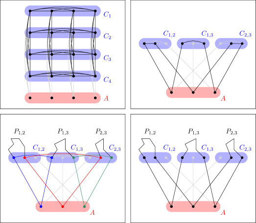
Figure 7: Four cases we encounter in the proof of Proposition 24.

If $\varphi(<,=)=\varphi(=,<)=1$ then for all $i,j,k,\ell\in[t_{0}]$ we have

$$(C_{i}(j),C_{k}(\ell))\in E(H)\iff(i=k\land j\neq\ell)\lor(i\neq k\land j=\ell).$$

The situation is depicted in the top-left panel of Figure 7. The graph induced on $\bigcup_{i\in[t_{0}]}C_{i}$ is therefore the rook graph of order $t_{0}$ and contains a $1$-flip of the $2$-web of order $t$ by Lemma 23. As $t\geqslant n$, our claim follows.

We now handle the remaining three cases. By picking an appropriate bijection $[t_{0}]\to[t]\times[t]$, relabel the sets $C_{i}$ with $i\in[t_{0}]$ as $C_{i,j}$ with $i,j\in[t]$. By an application of Ramsey’s theorem, there is a set $S$ of size $n$ such that for every $i,j\in S$ with $i<j$, the length of the path between $C_{i,j}(i)$ and $C_{i,j}(j)$ given by (R.4) is some fixed $r\in\{2,\ldots,\rho\}$. Write $P_{i,j}$ for the vertices appearing in the interior of this path. Thus far we have ensured that:

• the vertices $V\coloneqq\{A(i)\colon i\in S\}$ are independent;

• for all $i$ and $j<k<\ell$ belonging to $S$, there is an edge between $A(i)$ and $C_{j,k}(k)$ if and only if $k=i$, and an edge between $A(i)$ and $C_{k,\ell}(k)$ if and only if $k=i$.

• for all $i,j\in S$ with $i<j$, the vertices of $A(i),C_{i,j}(i),P_{i,j},C_{i,j}(j),A(j)$ form a path of length $r+2$;

• for $i<j$ and $k<\ell$ belonging to $S$ with $(i,j)\neq(k,\ell)$, there are no edges between the vertices in $P_{i,j}$ and $P_{k,\ell}$;

• the adjacency within $U\coloneqq\bigcup\left\{C_{i,j}(i),C_{i,j}(j)\colon i,j\in S,i<j\right\}$ depends on $\varphi$.

If $\varphi(<,=)=0$ and $\varphi(=,<)=1$ then for all $i<j$ from $S$ there is an edge $(C_{i,j}(i),C_{i,j}(j))$, while there are no edges between sets $C_{i,j}$ and $C_{k,\ell}$ for $(i,j)\neq(k,\ell)$. Then graph induced on $V\cup U$ is a $2$-subdivided clique of order $n$; see the top-right panel of Figure 7. If $\varphi(<,=)=1$ and $\varphi(=,<)=0$ then for all $i\in S$ the vertices $U_{i}\coloneqq\{C_{i,j}(i)\colon i,j\in S,i<j\}\cup\{C_{k,i}(i)\colon k,i,\in S,k<i\}\subseteq U$ form cliques, while there is no edge between $U_{i}$ and $U_{j}$ for $i\neq j$. It follows that the graph induced on $V\cup U\cup\bigcup\{P_{i,j}\colon i,j\in S,i<j\}$ is an $(r+1)$-web of order $n$; see the bottom-left panel of Figure 7. Finally, if $\varphi(<,=)=\varphi(=,<)=0$, then $U$ is an independent set. Then the graph induced on $V\cup U\cup\bigcup\{P_{i,j}\colon i,j\in S,i<j\}$ is an $(r+1)$-subdivided clique of order $n$; see the bottom-right panel of Figure 7. In either case, our claim follows. ∎

We are now in position to finish the proof of Theorem 4. For convenience we prove the following formulation, which is equivalent to Theorem 4 by negation.

Theorem 25.

A class of graphs $\mathscr{C}$ is monadically stable if and only if $\mathscr{C}$ is edge-stable and for every $k,r\geqslant 2$ the class $\mathscr{C}_{k}$ of $k$-flips from $\mathscr{C}$ does not contain arbitrarily large $r$-subdivided cliques or arbitrarily large $r$-webs as induced subgraphs.

Proof.

Trivially, if $\mathscr{C}$ is monadically stable then it is edge-stable, while for every $k\in\mathbb{N}$ the class $\mathscr{C}_{k}$ is also monadically stable. Since for any $r\geqslant 2$ the class of $r$-subdivided cliques and the class of $r$-webs are not monadically stable, these cannot occur as induced subgraphs of members of $\mathscr{C}_{k}$ for any $k\in\mathbb{N}$.

Conversely, assume that $\mathscr{C}$ is an edge-stable class of graphs that is not monadically stable. It follows by Theorem 22 that $\mathscr{C}$ admits rocket-patterns. Consequently, Proposition 24 implies that there are $k,r\geqslant 2$ such that $\mathscr{C}_{k}$ contains either arbitrarily large $r$-subdivided cliques or $r$-webs, as required. ∎

4.3 Hardness of model checking

In this section we establish hardness of first-order model checking for hereditary, edge-stable, non-monadically stable graph classes; that is, we prove Theorem 2, recalled below.

See 2

The main weight in the proof of Theorem 2 lies in a construction of an existential interpretation that interprets the class of all graphs in $\mathscr{C}$. To allow transferring complexity hardness results, this interpretation needs to be effective in the following sense.

Definition 10.

We say a class of graphs $\mathscr{C}$ effectively interprets a class $\mathscr{D}$, if there exists an interpretation $I$ and an algorithm which, given an input graph $H\in\mathscr{D}$, computes in polynomial time an output graph $G\in\mathscr{C}$ whose size is polynomial in $|V(H)|$, such that $I(G)=H$. We also say that $\mathscr{C}$ effectively existentially interprets $\mathscr{D}$ if the interpretation $I$ is existential.

First-order formulas can be naturally pushed through interpretations. More precisely, given an interpretation $I\coloneqq I_{\delta,\varphi}$ and a formula $\psi(\bar{x})$, we define $I(\psi)(\bar{x})$ to be the formula obtained by recursively rewriting $\psi$ where we replace each

• atomic subformula $E(x,y)$ with $\varphi(x,y)$,

• existential quantification $\exists z:\alpha(\bar{x},z)$ with $\exists z:\delta(z)\wedge\alpha(\bar{x},z)$, and

• universal quantification $\forall z:\alpha(\bar{x},z)$ with $\forall z:\delta(z)\rightarrow\alpha(\bar{x},z)$.

We have the following standard fact.

Fact 26 (see, e.g., [Hod97, Theorem 4.3.1]).

For every interpretation $I$, formula $\psi(\bar{x})$, graphs $G$ and $H$ satisfying $G=I(H)$, and tuple $\bar{a}\in V(G)^{|\bar{x}|}$,

$$G\models\psi(\bar{a})\qquad\textrm{if and only if}\qquad H\models I(\psi)(\bar{a}).$$

The next lemma formalizes the intuition that the hardness of first-order model checking can be pulled through effective interpretations.

Lemma 27.

Let $\mathscr{C}$ be a class of graphs that effectively interprets the class of all graphs. Then the first-order model checking problem is $\mathrm{AW[*]}$-hard on $\mathscr{C}$. If the interpretation is moreover existential, then existential first-order model checking on $\mathscr{C}$ is $\mathrm{W}[1]$-hard, and Induced Subgraph Isomorphism on $\mathscr{C}$ is $\mathrm{W}[1]$-hard with respect to Turing reductions.

Proof.

Let $I$ be an effective interpretation that interprets the class of all graphs from $\mathscr{C}$. It is immediate from 26 that the $\mathrm{AW[*]}$-hard first-order model checking problem on the class of all graphs can be reduced to the first-order model checking problem on $\mathscr{C}$.

If $I$ is moreover existential we reduce the $\mathrm{W[1]}$-hard Clique problem to the existential first-order model checking problem on $\mathscr{C}$. Given a graph $G$ and a parameter $k$, we can compute in polynomial time a graph $H\in\mathscr{C}$ such that $I(H)=G$. By 26 we have that $G$ contains a clique of size $k$ if and only if $H\models I(\psi)$, where

$$\psi\coloneqq\exists x_{1},\ldots,x_{k}:\bigwedge_{1\leqslant i<j\leqslant k}E(x_{i},x_{j}).$$

Note that since $I$ and $\psi$ are existential and $\psi$ does not contain any negations, we can compute an existential sentence equivalent to $I(\psi)$. This finishes the reduction.

Having shown that the existential first-order model checking problem is $\mathrm{W[1]}$-hard on $\mathscr{C}$, we Turing reduce it to the Induced Subgraph Isomorphism problem on $\mathscr{C}$ using the following standard construction. Let $\psi$ be an existential sentence using $k$ quantifiers. In time depending only on $k$ we can compute the set $\mathscr{D}$ of all graphs of size at most $k$ that model $\psi$. Now for every graph $G$, $G\models\psi$ if and only if $G$ contains a graph from $\mathscr{D}$ as an induced subgraph. ∎

Thus, Theorem 2 follows by combining Lemma 27 with the following statement, whose proof spans the remainder of this section.

Theorem 28.

Let $\mathscr{C}$ be a hereditary, edge-stable, non-monadically stable class of graphs. Then $\mathscr{C}$ effectively existentially interprets the class of all graphs.

Let us discuss our approach to the proof of Theorem 28. Recall that Theorem 25 implies that for any class $\mathscr{C}$ as above there are $k,r\geqslant 2$ such that $\mathscr{C}$ contains a $k$-flip of every $r$-subdivided clique, or $\mathscr{C}$ contains a $k$-flip of every $r$-web. It therefore suffices to show that each one of the two cases we may existentially interpret the class of all graphs on singletons. Despite the similarity between cliques and webs, we handle each one of these two cases individually as the two arguments rely on different structural properties of these patterns. Nonetheless, in both cases we shall consider the bipartite analogues of the patterns to simplify our arguments conceptually.

4.3.1 Hardness in webs

We first handle the case when the considered class contains a $k$-flip of every $r$-web. It will be convenient to conduct the reasoning on bipartite counterparts of webs, which we call biwebs; see Figure 8

Definition 11.

Given $r\geqslant 2$ and $n,m\in\mathbb{N}$ we define the $r$-biweb of order $(n,m)$, denoted by $W^{r}_{n,m}$ as the bipartite graph obtained by $r$-subdividing the complete bipartite graph $K_{n,m}$ and turning the neighborhood of each native vertex into a clique.

Figure 8: The graphs $W^{4}_{3,4}$ and $W^{6}_{5,4}$ respectively.

As is the case with subdivided bicliques and cliques, we may find biwebs within webs.

Observation 29.

For any $r\geqslant 2$ and $n\in\mathbb{N}$ the $r$-web $W^{r}_{2n}$ of order $2n$ contains the $r$-biweb $W^{r}_{n,n}$ of order $(n,n)$ as an induced subgraph.

Moreover, we may pass on to higher subdivision lengths from smaller ones.

Observation 30.

The biweb $W^{4}_{n,n}$ is an induced subgraph of $W^{2}_{n^{2},n^{2}}$.

With these observations at our disposal, we henceforth assume that $r\geqslant 3$ to simplify the proceeding arguments. Our main statement is the following.

Theorem 31.

Fix $r\geqslant 3$ and $k\in\mathbb{N}$. Let $\mathscr{C}$ be a hereditary class of graphs containing a $k$-flip of every $r$-biweb. Then $\mathscr{C}$ effectively interprets the class of all graphs using only existential formulas on singletons $\varphi(x,y)$ and $\delta(x)$ for the edge and domain formula.

We break down the interpretation into two parts. For fixed $t,r\in\mathbb{N}$, we let

$$\mathscr{W}^{r}_{t}\coloneqq\{H+W^{r}_{t,t}\colon\text{$H$ is an induced subgraph of some $r$-biweb}\},$$

where $+$ denotes the disjoint union of two graphs. Observe that if $\mathscr{C}$ is as in Theorem 31 then there is some $k\in\mathbb{N}$ such that the class $\mathscr{C}_{k}$ of all $k$-flips of graphs from $\mathscr{C}$ contains, as induced subgraphs, all of $\mathscr{W}^{r}_{t}$ for $t\in\mathbb{N}$. Our first lemma gives an existential interpretation in the case where there are no flips involved.

Lemma 32.

For every $r\geqslant 3$ and $t\geqslant 5$ the class $\mathscr{W}^{r}_{t}$ effectively existentially interprets the class of all graphs on singletons.

Proof.

Fix $r\geqslant 3$ and $t\geqslant 5$. Given an $n$-vertex graph $G$, we first describe the graph $f(G)\in\mathscr{W}^{r}_{t}$ that will perform the interpretation; see Figure 9. For every $v\in V(G)$, let $K^{v}$ be the graph obtained by taking $K_{4}$ and $K_{t+n}$, selecting an arbitrary vertex from $K_{4}$ and an arbitrary vertex from $K_{t+n}$, which we label $c_{v}$, and joining them by a path of length $r-1$. We then let $K^{V}$ be the disjoint union of $K^{v}$ over all $v\in V(G)$. Then, for every edge $uv\in E(G)$, we select an arbitrary vertex from the $(t+n)$-clique in $K^{v}$ which is not $c_{v}$, and an arbitrary vertex from the $(t+n)$-clique in $K^{u}$ which is not $c_{u}$, and join them by a path of length $2r-1$; moreover, vertices selected for different edges $uv\in E(G)$ are pairwise different. We write $B_{G}$ for the resulting graph. It is easy to see that $B_{G}$ is an induced subgraph of $W^{r}_{n+2,n+m+t}$ where $m\coloneqq|E(G)|$, and therefore $f(G)\coloneqq B_{G}+W^{r}_{t,t}\in\mathscr{W}^{r}_{t}$. Note that we add $2$ to the first dimension of the biweb to ensure that it is at least $3$ and we find $K_{4}$ as depicted in Figure 9. Moreover, $f(G)$ is clearly computable in polynomial time from $G$.

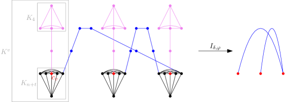
Figure 9: The graph $B_{G}$ constructed to interpret the graph $G$ on the right. The vertices are layouted to show how they embed into the layers of a $3$-biweb.

We proceed to define formulas $\delta(x)$ and $\varphi(x,y)$ for the domain and edge relation, respectively, of the interpretation. For the former, we first let $\chi(x)$ (for “kite”) be the existential formula that describes that there is an induced path of length $r-1$ starting at $x$ and leading to a clique of size $4$. We then let

$$\delta(x)\coloneqq\chi(x)\land\deg_{>t}(x),\qquad\varphi(x,y)\coloneqq\mathrm{dist}_{\leqslant 2r+1}(x,y),$$

where $\deg_{>t}(\cdot)$ and $\mathrm{dist}_{\leqslant 2r+1}(\cdot,\cdot)$ are existential formulas checking the degree and the distance, respectively. Evidently, both $\chi(x)$ and $\varphi(x,y)$ are existential formulas. It is now easy to see that for every graph $G$ we have $V(I_{\delta,\varphi}(f(G)))=\{c_{v}:v\in V(G)\}$ and $I_{\delta,\varphi}(f(G))$ is isomorphic to $G$. Hence, $I_{\delta,\varphi}$ is an interpretation of the class of all graphs in $\mathscr{W}^{r}_{t}$. ∎

To obtain an interpretation from $\mathscr{C}$ instead of $\mathscr{W}^{r}_{t}$, we would like to show that we can somehow definably “undo” the flip. More precisely, we aim to establish the following.

Theorem 33.

Fix $r\geqslant 3$ and $k\in\mathbb{N}$. Let $\mathscr{C}$ be a hereditary class of graphs containing a $k$-flip of every $r$-biweb. Then there exists some $t\geqslant 5$ such that for every existential formula $\varphi(\bar{x})$ there is an existential formula $\mathrm{flip}(\varphi)$, and for every graph $G\in\mathscr{W}^{r}_{t}$ there is a graph $\mathrm{flip}(G)\in\mathscr{C}$ which is a $k$-flip of $G$, so that

$$G\models\varphi(\bar{v})\qquad\textrm{if and only if}\qquad\mathrm{flip}(G)\models\mathrm{flip}(\varphi)(\bar{v}), *$$ ()

for all tuples $\bar{v}\in V(G)^{|\bar{x}|}$. Moreover, $\mathrm{flip}(G)$ can be computed from $G$ in polynomial time.

With this, Theorem 31 becomes an easy consequence.

Proof of Theorem 31 from Lemma 32 and Theorem 33.

Let $I=(\delta(x),\varphi(x,y))$ be the existential interpretation from Lemma 32, and let $t\in\mathbb{N}$ and $\mathrm{flip}(\cdot)$ be the integer and the operator given by Theorem 33. Consider the existential interpretation $J=(\mathrm{flip}(\delta),\mathrm{flip}(\varphi))$. Given an arbitrary graph $H$ there is, by Theorem 33, some $G\in\mathscr{W}^{r}_{t}$ such that $H$ is isomorphic to $I(G)$. By ($*$ ‣ 40), we know that $I(G)$ is isomorphic to $J(\mathrm{flip}(G))$. Since $\mathrm{flip}(G)\in\mathscr{C}$ can be computed from $H$ in polynomial time, this gives an effective existential interpretation of the class of all graphs in $\mathscr{C}$. ∎

The remainder of this section is therefore devoted to establishing Theorem 33.

Layers, colors, and flips.

Fix $r,k$ and $\mathscr{C}$ as in Theorem 33. For notational convenience we write $B_{n}\coloneqq W^{r}_{n,n}$. So, given an $r$-biweb $B_{n}$, we partition its vertices into $\ell\coloneqq r+2$ layers $\mathcal{L}\coloneqq\{L_{1},\ldots,L_{\ell}\}$ in the natural way: vertices of layer $L_{i}$ are those at distance $i-1$ from the native vertices on one side of biweb. Thus, $L_{1}\cup L_{\ell}$ are the native vertices on the opposite sides of the biweb. See the left side of Figure 10 for a visualization.

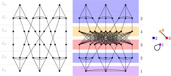
Figure 10: Left: a $4$-biweb partitioned into layers. Middle: a flip of a $4$-biweb partitioned into color classes. The exceptional colors in this example being $\mathbb{X}=\{2\}$. Right: The graph $\mathbf{M}$ depicting which color classes have been flipped.

By assumption, for every $n\in\mathbb{N}$, $\mathscr{C}$ contains a $k$-flip of $B_{n}$. Recall that this means that there is a coloring $\lambda_{n}\colon V(B_{n})\to[k]$ and a symmetric relation $R_{n}\subseteq[k]\times[k]$ such that $B_{n}\oplus_{\lambda_{n}}R_{n}\in\mathscr{C}$. By Ramsey’s theorem for bipartite graphs (see Lemma 19) and possibly restricting attention to a smaller biweb (recall that $\mathscr{C}$ is hereditary), we may assume that for every length-$(r+1)$ path between native vertices on opposite sides of $B_{n}$, the sequence of colors assigned by $\lambda_{n}$ to the vertices of this path is the same. Also, by pigeonhole principle we may assume that these sequences of colors are equal for all $n\in\mathbb{N}$, and also that all relations $R_{n}$ for $n\in\mathbb{N}$ are equal. All in all, these assumptions yield the following: there exist a number of colors $c\leqslant\min\{\ell,k\}$, a surjective mapping $\mathrm{lc}\colon\mathcal{L}\to[c]$ (for layer color), and a symmetric relation $R\subseteq[c]^{2}$ with the following property.

For every $r$-biweb $B_{n}$, let $\lambda$ be the $c$-coloring of $V(B_{n})$ in which each layer $L\in\mathcal{L}$ is monochromatic and has color $\mathrm{lc}(L)$. Note that two different layers might be assigned the same color. See middle of Figure 10 for a visualization.

Define $\mathrm{flip}(B_{n})\coloneqq B_{n}\oplus_{\lambda}R$. Then we have that $\mathrm{flip}(B_{n})$ is contained in $\mathscr{C}$.

Let now $\mathbf{M}$ be the graph with vertex set $[c]$ and edge set $R$. We consider $\mathbf{M}$ as a graph possibly with loops: there is a loop at $i\in[c]$ if $(i,i)\in R$. The neighborhood of $i$ is defined as $N_{\mathbf{M}}(i)\coloneqq\{j\in[c]~{}|~{}(i,j)\in R\}$; note that $i\in N_{\mathbf{M}}(i)$ if there is a loop at $i$. Distinct $i,j\in[c]$ are called twins if $N_{\mathbf{M}}(i)=N_{\mathbf{M}}(j)$. Note that if there are twins in $\mathbf{M}$, then the corresponding colors can be merged in the mapping $\mathrm{lc}$, hence we may assume the following:

The number of colors $c$ is minimal: the graph $\mathbf{M}$ contains no twins.

Note that this entails the following: for all distinct $i,j\in[c]$, the symmetric difference

$$\triangle_{\mathbf{M}}(i,j)\coloneqq\left(N_{\mathbf{M}}(i)-N_{\mathbf{M}}(j)\right)\cup\left(N_{\mathbf{M}}(j)-N_{\mathbf{M}}(i)\right)$$

of the neighborhoods of $i$ and $j$ in $\mathbf{M}$ is always non-empty. See right side of Figure 10 for a visualization.

Having fixed $\mathrm{lc}$, we will from now on assume that any $r$-biweb is implicitly $c$-colored. For every induced subgraph $H$ of $B_{n}$ we define $\mathrm{flip}(H)$ to be the graph induced by $V(H)$ in $\mathrm{flip}(B_{n})$. Our notion of layers and colors carries over to $\mathrm{flip}(B_{n})$, $H$, and $\mathrm{flip}(H)$ in the obvious way. In every $r$-biweb $B_{n}$, the layers $L_{2}$ and $L_{\ell-1}$ are the only layers containing cliques. We will refer to those cliques as cones. Hence, $B_{n}$ contains $2n$ cones: $L_{2}$ and $L_{\ell-1}$ each contain $n$ cones. We will later use the cones to distinguish the exceptional layers $L_{2}$ and $L_{\ell-1}$ from the non-exceptional layers $\mathcal{L}-\{L_{2},L_{\ell-1}\}$. We call the set $\mathbb{X}\coloneqq\{\mathrm{lc}(L_{2}),\mathrm{lc}(L_{\ell-1})\}$ the exceptional colors. As both exceptional layers can possibly be assigned to the same color, we have $|\mathbb{X}|\in\{1,2\}$.

Our aim is to find some $t\in\mathbb{N}$ such that for every $G\coloneqq H+B_{t}\in\mathscr{W}^{r}_{t}$ we may definably recover the color of each vertex $v\in V(G)$ by looking at the adjacency in $\mathrm{flip}(G)$ between $v$ and certain carefully picked subsets of $\mathrm{flip}(B_{t})$. Since we are not allowed to treat $\mathrm{flip}(B_{t})$ as a tuple of parameters in our formula, we have to existentially quantify over some subset of $G$ that induces a graph isomorphic to $\mathrm{flip}(B_{t})$. However, it is possible that this captures a different copy of $\mathrm{flip}(B_{t})$ within $\mathrm{flip}(G)$, rather than the intended one. Our aim is to establish that, even in this case, we can recover the color of a vertex by its adjacency to this existentially quantified subgraph.

Therefore, in proving Theorem 33 we describe quantifier free formulas $\mathrm{check}(\bar{z})$ and $E_{0}(x,y,\bar{z})$ which specify the following rewriting procedure. For every formula $\varphi(\bar{x})$ define

$$\mathrm{flip}(\varphi)(\bar{x})\coloneqq\exists\bar{z}(\mathrm{check}(\bar{z})\wedge\hat{\varphi}(\bar{x},\bar{z})),$$

where $\hat{\varphi}$ is obtained from $\varphi$ by replacing every occurrence of $E(x,y)$ with $E_{0}(x,y,\bar{z})$. The goal is to choose $\mathrm{check}(\bar{z})$ and $E_{0}(x,y,\bar{z})$ in a way that ensures ($*$ ‣ 40). As we demand $\mathrm{check}(\bar{z})$ and $E_{0}(x,y,\bar{z})$ to be quantifier-free, then $\mathrm{flip}(\varphi)$ will be existential, provided that $\varphi$ is.

Defining the interpretation.

For a sufficiently large $t\in\mathbb{N}$ that remains to be specified, let $(w_{1},\ldots,w_{q})$ be an arbitrary enumeration of the vertices of $B_{t}$, where $q\coloneqq|B_{t}|$. Letting $\bar{z}=(z_{1},\ldots,z_{q})$ be a $q$-tuple of variables, the formula $\mathrm{check}(\bar{z})$ will check whether the vertices $\bar{z}$ induce $\mathrm{flip}(B_{t})$ as a subgraph. More precisely, we choose $\mathrm{check}(\bar{z})$ as the conjunction of atomic and negated atomic formulas capturing the adjacency within $\mathrm{flip}(B_{t})$, so that for every graph $G$ and tuple $\bar{a}=(a_{1},\ldots,a_{q})\in V(G)^{q}$ we have

$$G\models\mathrm{check}(\bar{a})\quad\Leftrightarrow\quad\text{$\{a_{i}\mapsto w_{i}\colon i\in[c]\}$ is an isomorphism from $G[\bar{a}]$ to $\mathrm{flip}(B_{t})$.}$$ (5)

We now carefully select disjoint subsets $Z_{1},\ldots,Z_{c}$ of the variables of $\bar{z}$. Intuitively, we want the adjacency between a vertex $v$ and the realization of these variables to determine the color of $v$. Pick odd $s\in\mathbb{N}$ so that

$$s\geqslant 8c\ell.$$

For every $i\in[c]$, let $W_{i}\coloneqq\{w_{j}\colon z_{j}\in Z_{i}\}$ be the vertices from $\mathrm{flip}(B_{t})$ to which valuations of $Z_{i}$ are mapped by the isomorphism from (5). Then we select $Z_{1},\ldots,Z_{c}$ so that for every $i\in[c]$, we have the following.

1. $W_{i}$ is contained in a single layer $L$ of $\mathrm{flip}(B_{t})$ satisfying $\mathrm{lc}(L)=i$.

2. $W_{i}$ has size $s^{2}$.

3. If $i\in\mathbb{X}$, then the $s^{2}$ vertices from $W_{i}$ are chosen to be $s$ batches of $s$ vertices, where each batch contained in a different cone. In particular $W_{i}$ induces in $\mathrm{flip}(B_{t})$ either

   • $sK_{s}$: the disjoint union of $s$ cliques of size $s$ each, or (this happens if $(i,i)\notin R$)

   • $\overline{sK_{s}}$: the complement of the above. (this happens if $(i,i)\in R$)

4. If $i\not\in\mathbb{X}$, then $W_{i}$ induces in $\mathrm{flip}(B_{t})$ either

   • an independent set, or (this happens if $(i,i)\notin R$)

   • a clique. (this happens if $(i,i)\in R$)

5. For all $j\in[c]-\{i\}$, the bipartite graph semi-induced between $W_{i}$ and $W_{j}$ in $\mathrm{flip}(B_{t})$ is either

   • anti-complete, or (this happens if $(i,j)\notin R$)

   • complete. (this happens if $(i,j)\in R$)

Let us verify that such a selection is indeed possible, supposing $t$ is large enough.

Claim 5.

Assuming $t\geqslant cs^{2}$, there are sets $W_{1},\dots,W_{c}$ from $\mathrm{flip}(B_{t})$ satisfying the properties above.

Proof.

As $\mathrm{flip}(B_{t})$ and $B_{t}$ have the same vertex set, we will describe how to choose the desired vertices in the latter. More precisely, we choose $W_{1},\ldots,W_{c}$ from the graph $cB_{s^{2}}$, that is, the disjoint union of $c$ $r$-biwebs of order $s^{2}$ each. It is easy to see that $cB_{s^{2}}$ is an induced subgraph of $B_{cs^{2}}$, which in turn is contained in $B_{t}$ under our assumption on $t$. For each color $i\in[c]$ we will choose $W_{i}$ by picking $s^{2}$ vertices from layer $L(i)$ of the $i$th copy of $B_{s^{2}}$, where $L(i)$ is an arbitrary layer such that $\mathrm{lc}(L(i))=i$ and $L(i)$ is exceptional if $i\in\mathbb{X}$. See Figure 11 for a visualization.

Figure 11: A depiction of how the sets $W_{i}$ embed into multiple copies of $B_{s^{2}}$. For the sake of clarity, the sizes of the sets were not chosen faithfully.

It is easy to check that each layer in $B_{s^{2}}$ contains at least $s^{2}$ vertices, so this is possible. The $W_{i}$ picked this way satisfy (P.$1$) and (P.$2$) by definition. To check (P.$3$) - (P.$5$), we analyze the adjacencies of the sets in $\mathrm{flip}(B_{t})$. As we picked all $W_{i}$ from disjoint copies, they are pairwise anti-complete to each other in $B_{t}$. As each $W_{i}$ is monochromatic, we know that in $\mathrm{flip}(B_{t})$ their pairwise adjacencies remain homogeneous and (P.$5$) is satisfied. It remains to show (P.$4$) and (P.$3$). If $i\notin\mathbb{X}$ then $W_{i}$ was picked from a non-exceptional layer from the $i$th copy of $B_{s^{2}}$. This layer is an independent set in $B_{t}$ and as $W_{i}$ is monochromatic, (P.$4$) follows. If $i\in\mathbb{X}$ then $W_{i}$ was picked from an exceptional layer $L(i)$ from the $i$th copy of $B_{s^{2}}$. $L(i)$ induces $s^{2}K_{s^{2}}$ in $B_{t}$, so it is therefore possible to choose $W_{i}$ to induce $sK_{s}$ in $B_{t}$. As $W_{i}$ is monochromatic, (P.$3$) follows. ∎

Since the variables of $\mathrm{check}(\bar{z})$ are in 1-1 correspondence with the vertices of $\mathrm{flip}(B_{t})$, the sets $W_{i}\subseteq V(B_{t})$ uniquely specify the sets $Z_{i}$ of variables of $\bar{z}$. Having fixed the variables $Z_{1},\dots,Z_{c}$ among $\bar{z}$, for each $i\in[c]$ we define $\mathrm{predictedCol}_{i}(x,\bar{z})$ to be the quantifier-free formula checking whether

$$\{j\in[c]\colon\text{$x$ is adjacent to at least half of the vertices of $Z_{j}$}\}=N_{\mathbf{M}}(i).$$

This may be easily defined by making a disjunction over all the possible ways that $x$ could be adjacent to the majority of $Z_{j}$, for all $j\in[c]$ such that $(i,j)\in R$, and non-adjacent to the majority of $Z_{j^{\prime}}$, for all $j^{\prime}\in[c]$ such that $(i,j^{\prime})\notin R$.

The benefit of this majority-type argument is that, even if $\mathrm{check}(\bar{z})$ does not capture the intended copy of $\mathrm{flip}(B_{t})$ within $\mathrm{flip}(G)$, we can still determine the color of a vertex, possibly after some automorphism of the flip relation. This observation is captured by the following claim, which is the crux of our approach.

Claim 6.

For every induced subgraph $G$ of an $r$-biweb and tuple $\bar{a}$ from $G$ satisfying $\mathrm{flip}(G)\models\mathrm{check}(\bar{a})$, there exists an automorphism $f_{\star}$ of $\mathbf{M}$ such that for every vertex $v$ in $G$ and $i\in[c]$,

$$v f_{\star}(i) \mathrm{flip}(G)\models\mathrm{predictedCol}_{i}(v,\bar{a})$$ has color   if and only if  .

We postpone the proof of this claim for now; it will be given further ahead. Instead, we proceed with defining $E_{0}(x,y,\bar{z})$ assuming that Claim 6 is established.

Towards this, we first define a quantifier-free formula $\mathrm{flipped}(x,y,\bar{z})$ which detects whether the connection between $x$ and $y$ was flipped. More concretely, we let

$$\mathrm{flipped}(x,y,\bar{z})\coloneqq\bigvee_{i,j\in[c]}\mathrm{predictedCol}_{i}(x,\bar{z})\wedge\mathrm{predictedCol}_{j}(y,\bar{z})\wedge\bigl{(}(i,j)\in R\bigr{)}.$$

As $c$ and $R$ are fixed, $\mathrm{flipped}(x,y,\bar{z})$ is once again a single quantifier-free formula. We argue that this formula does indeed behave in the intended way.

Claim 7.

For every $G\in\mathscr{W}^{r}_{t}$, tuple $\bar{a}\in V(G)^{q}$ satisfying $\mathrm{flip}(G)\models\mathrm{check}(\bar{a})$ and vertices $u,v\in V(G)$,

$$\mathrm{flip}(G)\models\mathrm{flipped}(u,v,\bar{a})\qquad\textrm{if and only if}\qquad\text{$u$ and $v$ are adjacent in exactly one of $G$ and $\mathrm{flip}(G)$.}$$

Proof.

By the definition of $\mathrm{flipped}(x,y,\bar{z})$ we have

$$\mathrm{flip}(G)\models\mathrm{flipped}(u,v,\bar{a})\quad\Leftrightarrow\quad\bigvee_{i,j\in[c]}\mathrm{predictedCol}_{i}(u,\bar{a})\wedge\mathrm{predictedCol}_{j}(v,\bar{a})\wedge\bigl{(}(i,j)\in R\bigr{)}.$$

Assume $\mathrm{flip}(G)\models\mathrm{flipped}(u,v,\bar{a})$. Then there exist $i,j\in[c]$ such that

$$\mathrm{flip}(G)\models\mathrm{predictedCol}_{i}(u,\bar{z})\wedge\mathrm{predictedCol}_{j}(v,\bar{z})\wedge\bigl{(}(i,j)\in R\bigr{)}.$$

By Claim 6, there exists an automorphism $f_{\star}$ on $\mathbf{M}$ such that $u$ and $v$ have color $f_{\star}(i)$ and $f_{\star}(j)$ respectively. As $f_{\star}$ is an automorphism, $(i,j)\in R$ implies that $(f_{\star}(i),f_{\star}(j))\in R$. Hence, the adjacency between $u$ and $v$ was flipped from $G$ to $\mathrm{flip}(G)$ as desired.

On the other hand, assume $\mathrm{flip}(G)\not\models\mathrm{flipped}(u,v,\bar{a})$. Then for all $i,j\in[c]$

$$\mathrm{flip}(G)\not\models\mathrm{predictedCol}_{i}(u,\bar{z})\wedge\mathrm{predictedCol}_{j}(v,\bar{z})\wedge\bigl{(}(i,j)\in R\bigr{)}.$$

Since $f_{\star}$ is an automorphism, there exist $i,j\in[c]$ such that $u$ and $v$ have color $f_{\star}(i)$ and $f_{\star}(j)$ respectively. By Claim 6, we have

$$\mathrm{flip}(G)\models\mathrm{predictedCol}_{i}(u,\bar{z})\wedge\mathrm{predictedCol}_{j}(v,\bar{z})\quad\text{ and consequently }\quad(i,j)\notin R.$$

Again using the fact that $f_{\star}$ is an automorphism, we have $(f_{\star}(i),f_{\star}(j))\notin R$. Then the adjacency between $u$ and $v$ was not flipped from $G$ to $\mathrm{flip}(G)$ as desired. ∎

It is easy to see that with the formula $\mathrm{flipped}(x,y,\bar{z})$ at our disposal, the formula

$$E_{0}(x,y,\bar{z})\coloneqq E(x,y)\text{ XOR }\mathrm{flipped}(x,y,\bar{z})$$

has the desired properties. Recall that given a formula $\varphi$ in the language of graphs, we write $\hat{\varphi}$ for the formula obtained by replacing every $E(x,y)$ atom by $E_{0}(x,y,z)$.

Claim 8.

For all $G\in\mathscr{W}^{r}_{t}$, formulas $\varphi(\bar{x})$, and tuples $\bar{v}$ from $V(G)^{|\bar{x}|}$ the following are equivalent:

1. $G\models\varphi(\bar{v})$;

2. $\mathrm{flip}(G)\models\forall\bar{z}(\mathrm{check}(\bar{z})\to\hat{\varphi}(\bar{v},\bar{z}))$;

3. $\mathrm{flip}(G)\models\exists\bar{z}(\mathrm{check}(\bar{z})\land\hat{\varphi}(\bar{v},\bar{z}))\quad(=\mathrm{flip}(\varphi)(\bar{v}))$.

Proof.

We handle the case where $\varphi(x,y)\coloneqq E(x,y)$; the rest follows by induction on the structure of $\varphi$. Fix $u,v\in V(G)$. Suppose that $G\models E(u,v)$ and let $\bar{a}\in V(G)^{|\bar{z}|}$ such that $\mathrm{flip}(G)\models\mathrm{check}(\bar{a})$. If the edge $(u,v)$ was flipped from $G$ to $\mathrm{flip}(G)$ then by construction $\mathrm{flip}(G)\models\neg E(u,v)\land\mathrm{flipped}(u,v,\bar{a})$. Consequently, $\mathrm{flip}(G)\models E_{0}(u,v,\bar{a})$. If the edge $(u,v)$ was not flipped from $G$ to $\mathrm{flip}(G)$ then $\mathrm{flip}(G)\models E(u,v)\land\neg\mathrm{flipped}(u,v,\bar{a})$, and so $\mathrm{flip}(G)\models E_{0}(u,v,\bar{a})$. This shows $\ref{itm:qf}\implies\ref{itm:uni}$.

Suppose that $\mathrm{flip}(G)\models\forall\bar{z}(\mathrm{check}(\bar{z})\to E_{0}(u,v,\bar{z}))$. Letting $\bar{w}$ be the enumeration of the vertices in $B_{t}$, we see that $\mathrm{flip}(G)\models\mathrm{check}(\bar{w})\land E_{0}(u,v,\bar{w})$. Consequently, $\mathrm{flip}(G)\models\exists\bar{z}(\mathrm{check}(\bar{z})\land E_{0}(u,v,\bar{z}))$ and so $\ref{itm:uni}\implies\ref{itm:ex}$.

Finally, assume that $\mathrm{flip}(G)\models\exists\bar{z}(\mathrm{check}(\bar{z})\land E_{0}(u,v,\bar{z}))$ and let $\bar{a}\in V(G)^{|\bar{z}|}$ be the tuple witnessing this. Assume that $\mathrm{flip}(G)\models E(u,v).$ It follows that $\mathrm{flip}(G)\models\neg\mathrm{flipped}(u,v,\bar{a})$ and so the edge $(u,v)$ was not flipped from $G$ to $\mathrm{flip}(G)$; hence $G\models E(u,v)$. On the other hand, if $\mathrm{flip}(G)\models\neg E(u,v)$ then $\mathrm{flip}(G)\models\mathrm{flipped}(u,v,\bar{a})$ and so the edge $(u,v)$ was flipped; it follows that $G\models E(u,v)$. This implies that $3\implies 1$. ∎

Noting that the third formula was precisely defined to be $\mathrm{flip}(\varphi)$, Theorem 33 follows directly from the above. Note that we set $t\coloneqq cs^{2}$ so that Claim 5 holds.

Proof of Claim 6

We now proceed to the proof of Claim 6, which we restate below for convenience. In the following statement and proof, our setup is precisely the same as before.

See 6

We henceforth fix an induced subgraph $G$ of an $r$-web, and a tuple $\bar{a}=(a_{1},\dots,a_{q})\in V(G)^{q}$ such that $\mathrm{flip}(G)\models\mathrm{check}(\bar{a})$. For every $i\in[c]$, let $A_{i}\coloneqq\{a_{j}\colon z_{j}\in Z_{i}\}\subseteq V(G)$ be the valuations of the variables in $Z_{i}$. As $\mathrm{flip}(G)\models\mathrm{check}(\bar{a})$, there is an isomorphism from $\mathrm{flip}(G)[\bar{a}]$ to $\mathrm{flip}(B_{t})$ that maps $A_{i}$ to $W_{i}$. It follows that the properties (P.$2$) - (P.$5$), which determine the structure induced by the vertices $W_{i}$ in $\mathrm{flip}(B_{t})$, carry over to the vertices $A_{i}$ in $\mathrm{flip}(G)$. However, a priori we cannot guarantee a property in the spirit of (P.$1$) for the $A_{i}$. We know that $\bar{a}$ is some embedding of $\mathrm{flip}(B_{t})$ in $\mathrm{flip}(G)$, but we do not know from which layers of $\mathrm{flip}(G)$ the vertices in $\bar{a}$ and its $A_{i}$ subsets were chosen.

The main idea of the proof is that sets $A_{i}$ are chosen large enough that by pigeonhole principle, they will contain large subsets that will faithfully “represent” different colors. Precisely, our analysis will be based on the following definition.

Definition 12.

A function $f\colon[c]\to[c]$ is popular if for every $i\in[c]$, $A_{i}$ contains at least $\frac{1}{4c}|A_{i}|=\frac{1}{4c}s^{2}$ vertices of color $f(i)$.

Note that the pigeonhole principle implies that there is always a popular function $f$, and this would hold even if we relaxed the $\frac{1}{4c}s^{2}$ bound to $\frac{1}{c}s^{2}$. We weaken the bound deliberately for technical reasons. Surprisingly, we will establish that any popular function $f\colon[c]\to[c]$ actually gives an automorphism of the graph $\mathbf{M}$. Towards this, we make a sequence of observations about the structure of the sets $A_{i}$ and properties of popular functions.

Observation 34.

In $G$ no vertex contains in its neighborhood an induced $2K_{2}$ or $\overline{2K_{2}}$.

Observation 35.

Every non-exceptional layer induces an independent set or a clique in $\mathrm{flip}(G)$.

Observation 36.

Let $x\in\mathbb{X}$. Every subset of $A_{x}$ of size $2s$ contains vertices inducing in $\mathrm{flip}(G)$

• $2K_{2}$, if $(i,i)\notin R$, or

• $\overline{2K_{2}}$, if $(i,i)\in R$.

The previous two observations combined with the pigeonhole principle give the following.

Observation 37.

Let $x\in\mathbb{X}$. $A_{x}$ contains less than $(\ell-2)\cdot 2s$ vertices from non-exceptional layers.

We shall also make use of the following claim in our arguments.

Claim 9.

Let $i,j\in[c]$ be distinct. Then for all $4$-element subsets $V_{i}\subseteq A_{i}$ and $V_{j}\subseteq A_{j}$, there is a $4$-element set $V_{ij}\subseteq V(G)$ such that

1. $V_{ij}$ is disjoint from $V_{i}$ and $V_{j}$;

2. $V_{ij}$ is homogeneous to $V_{i}$ in $\mathrm{flip}(G)$;

3. $V_{ij}$ is homogeneous to $V_{j}$ in $\mathrm{flip}(G)$;

4. $V_{ij}$ is inhomogeneous to $V_{i}\cup V_{j}$ in $\mathrm{flip}(G)$; and

5. $V_{ij}$ is contained in a single layer in $\mathrm{flip}(G)$.

Proof.

We show the existence of a set $V_{ij}$ of size $4\ell$ which satisfies the first four properties. By the pigeonhole principle, we then find a set satisfying all properties. Choose any $d\in\triangle_{\mathbf{M}}(i,j)$. (Recall here that $\triangle_{\mathbf{M}}(i,j)$ is non-empty by the assumption that $\mathbf{M}$ has no twins.)

First assume $d=i$ and $(i,d)\notin R\ni(j,d)$. Then either

• $i\in\mathbb{X}$ and $A_{i}$ induces $sK_{s}$ in $\mathrm{flip}(G)$, or (by (P.$3$))

• $i\notin\mathbb{X}$ and $A_{i}$ induces an independent set in $\mathrm{flip}(G)$. (by (P.$4$))

In both cases, as $s\geqslant 8k\ell$ and so in particular $s\geqslant 4\ell+4$, we find a set $V_{ij}$ in $A_{i}$ which is disjoint from and non-adjacent to $V_{i}$. By (P.$5$), $v$ is adjacent to all of $A_{j}$ including $V_{j}$ and $V_{ij}$ has the desired properties.

If $d=i$ but instead $(i,d)\in R\not\ni(j,d)$, we argue as before exchanging cliques with independent sets and adjacencies with non-adjacencies. If $d=j$, we argue by symmetry. If $d\notin\{i,j\}$, we argue by (P.$5$). This exhausts all cases. ∎

With all the above, we now proceed to establishing that every popular function is in fact an automorphism of $\mathbf{M}$.

Claim 10.

For every popular function $f$, $f|_{\mathbb{X}}$ is a bijection from $\mathbb{X}$ to $\mathbb{X}$.

Proof.

Assume first there is only a single exceptional color: $\mathbb{X}=\{x\}$. By popularity, $A_{x}$ contains at least $\frac{1}{4c}s^{2}$ vertices of color $f(x)$. By 37, there must be a vertex from an exceptional layer with color $f(x)$, since $(\ell-2)\cdot 2s\leqslant\frac{1}{4c}s^{2}$. It follows that $f(x)\in\mathbb{X}$ so $f(x)=x$, and we are done.

Assume now there are two exceptional colors: $\mathbb{X}=\{x_{1},x_{2}\}$. Following the previous case, we know $f(x_{1})\in\mathbb{X}$ and $f(x_{2})\in\mathbb{X}$ and it remains to show $f(x_{1})\neq f(x_{2})$. Assume towards a contradiction that $f(x_{1})=f(x_{2})$. Let $V^{\prime}_{1}\subseteq A_{x_{1}}$ and $V^{\prime}_{2}\subseteq A_{x_{2}}$ be the two sets of size $\frac{s^{2}}{4c}$ which both have color $f(x_{1})$. By 36, we find subsets $V_{1}\subseteq V_{1}^{\prime}$ and $V_{2}\subseteq V_{2}^{\prime}$ which both either induce $2K_{2}$ or $\overline{2K_{2}}$ in $\mathrm{flip}(G)$; here we use $2s\leqslant\frac{1}{4c}s^{2}$. Claim 9 yields a vertex $v$ which is homogeneous to $V_{1}$ and homogeneous to $V_{2}$ but inhomogeneous to $V_{1}\cup V_{2}$ and not included in any of the sets. As $V_{1}$ and $V_{2}$ have the same color, no matter the choice of $R$, in the non-flipped graph $G$ the vertex $v$ is adjacent to either all of $V_{1}$ or all of $V_{2}$. Now 34 yields a contradiction ∎

Claim 11.

For every popular function $f$ and all $i\notin\mathbb{X}$, we have $f(i)\notin\mathbb{X}$.

Proof.

By Claim 10, for every $x^{\prime}\in\mathbb{X}$, there exists an $x\in\mathbb{X}$ with $f(x)=x^{\prime}$. To prove the claim it therefore suffices to show that for all $i\notin\mathbb{X}$ and $x\in\mathbb{X}$: $f(i)\neq f(x)$. Assume towards a contradiction that there is a color $d\in[c]$ with $d=f(i)=f(x)$. Since $2s\leqslant\frac{1}{4c}s^{2}$, there exists a size four subset $V_{x}\subseteq A_{x}$ such that

• $V_{x}$ either induces $2K_{2}$ or $\overline{2K_{2}}$ in $\mathrm{flip}(G)$; and (by 36)

• all vertices in $V_{x}$ have color $d$. (by popularity)

Let $V_{i}$ be a size four subset from a single layer and of color $d$ from $A_{i}$; such $V_{i}$ exists due to $4\leqslant\frac{s^{2}}{4c\ell}$. We obtain $V_{ix}$ by applying Claim 9 to $V_{i}$ and $V_{x}$.

Recall that $V_{ix}$ is inhomogeneous to $V_{i}\cup V_{x}$, but homogeneous to each of $V_{i}$ and $V_{x}$ separately. Since both $V_{ix}$ and $V_{i}\cup V_{x}$ are monochromatic, this conclusion also holds in graph $G$. By 34, $V_{ix}$ cannot be complete to $V_{x}$ in $G$, for $V_{x}$ induces $2K_{2}$ or $\overline{2K_{2}}$ in $\mathrm{flip}(G)$, so also in $G$. Hence in $G$, $V_{ix}$ must be anti-complete to $V_{x}$ and complete to $V_{i}$.

By the structure of a biweb, $V_{i}$ and $V_{ix}$ must form a clique and are located in the same exceptional layer in $G$. Recall that there is an isomorphism from $\mathrm{flip}(G)[\bar{a}]$ to $\mathrm{flip}(B_{t})$ which maps $A_{i}$ to $W_{i}$. By $i\notin\mathbb{X}$ and (P.$1$), $W_{i}$ is contained in a single non-exceptional layer $L$ in $\mathrm{flip}(B_{t})$. Analyzing the structure of the non-flipped biweb $B_{t}$, it is easy to see that for every vertex $u$ in $W_{i}$ there exist two distinct vertices $v_{1},v_{2}$ whose only neighbor in the layer $L$ is $u$. Lifting this fact through the flip to $\mathrm{flip}(B_{t})$ and through the isomorphism to $\mathrm{flip}(G)[\bar{a}]$, we obtain that for every vertex $u\in A_{i}$, there exist two distinct vertices $v_{1},v_{2}$ with the following property. In $\mathrm{flip}(G)$, each of $v_{1},v_{2}$ is either

1. adjacent to $u$ and non-adjacent to all other vertices from $V_{i}\subseteq A_{i}$, or

2. non-adjacent to $u$ and adjacent to all other vertices from $V_{i}\subseteq A_{i}$.

$V_{i}$ is monochromatic by assumption. As the vertices $v_{1}$ and $v_{2}$ are singletons, each of them is trivially monochromatic, too. It follows that the adjacency between each of $v_{1}$ and $v_{2}$ and $V_{i}$ in $G$ is the same as in either $\mathrm{flip}(G)$ or its complement. Since also the cases (C.$1$) and (C.$2$) are complementary, they also describe the connection of $v_{1}$ and $v_{2}$ towards $V_{i}$ in the non-flipped graph $G$. Recall that $V_{i}$ forms a clique in $G$ and fix a vertex $u\in V_{i}$. Let $v_{1},v_{2}$ be the two distinct vertices satisfying either (C.$1$) or (C.$2$). Depending on which of the two cases applies for each vertex and whether $v_{1}$ and $v_{2}$ are connected, $G$ contains one of the three graphs listed in Figure 12, none of which is contained in $G$ as an induced subgraph. We have reached the desired contradiction. ∎

Figure 12: Three induced subgraphs that cannot appear in an $r$-biweb.

Claim 12.

Every popular function $f$ is a strong homomorphism from $\mathbf{M}$ to $\mathbf{M}$:

$$\forall i,j\in[c]:\quad(i,j)\in R\Leftrightarrow(f(i),f(j))\in R.$$

Proof.

We do a case analysis.

Case 1: $i=j$ and $i\in\mathbb{X}$. As $2s\leqslant\frac{1}{4c}s^{2}$, popularity and 36 imply that the color class $f(i)$ contains four vertices that induce ${2K_{2}}$ in $\mathrm{flip}(G)$ if $(i,i)\notin R$ or $\overline{2K_{2}}$ if $(i,i)\in R$. Since $\overline{2K_{2}}$ is not an induced subgraph of $G$, we have that the color class $f(i)$ was flipped if and only if $i$ was, that is, $(f(i),f(i))\in R\iff(i,i)\in R$.

Case 2: $i=j$ and $i\notin\mathbb{X}$. By popularity, Claim 11, and (P.$4$), the color class $f(i)$ contains four vertices from non-exceptional layers, that induce and independent set if $(i,i)\notin R$ or a clique if $(i,i)\in R$ in $\mathrm{flip}(G)$; here we use that $4\leqslant\frac{1}{4c}s^{2}$. Since the non-exceptional layers in $G$ contain no clique of size four, we have that the color class $f(i)$ was flipped if and only if $i$ was, that is, $(f(i),f(i))\in R\iff(i,i)\in R$.

Case 3: $i\neq j$ and at least one of $i$ and $j$ is contained in $\mathbb{X}$. By symmetry, we can assume $i$ is contained in $\mathbb{X}$. By popularity and 36, the color class $f(i)$ contains a four vertex set $V_{i}$ that induces ${2K_{2}}$ or $\overline{2K_{2}}$ in $\mathrm{flip}(G)$; here we use that $2s\leqslant\frac{1}{4c}s^{2}$. As $V_{i}$ is monochromatic the same holds in $G$. By popularity and (P.$5$), $A_{j}$ contains a vertex $v$ with color $f(j)$ that is adjacent to all of $V_{i}$ in $\mathrm{flip}(G)$ if $(i,j)\in R$ or adjacent to none of $V_{i}$ in $\mathrm{flip}(G)$ if $(i,j)\notin R$. We now derive $(i,j)\in R\Leftrightarrow(f(i),f(j))\in R$ from 34.

Case 4: $i\neq j$ and none of $i$ and $j$ is contained in $\mathbb{X}$. By popularity and Claim 11, there exist two four element subsets $S_{i}\subseteq A_{i}$ and $S_{j}\subseteq A_{j}$ with color $f(i)$ and $f(j)$ respectively, none of which contains vertices from exceptional layers; here we use that $4\leqslant\frac{1}{4c}s^{2}$. By (P.$5$), $S_{i}$ and $S_{j}$ are either anti-complete or complete to each other in $\mathrm{flip}(G)$ depending on whether $(i,j)\in R$. Since the non-flipped graph $G$ contains no semi-induced bicliques of order four between vertices of non-exceptional layers, we conclude $(i,j)\in R\Leftrightarrow(f(i),f(j))\in R$.

This exhausts all cases. ∎

Claim 13.

Every popular function $f$ is an automorphism on $\mathbf{M}$.

Proof.

It remains to show that $f$ is injective. Assume towards a contradiction that there are $i\neq j$ both not in $\mathbb{X}$ such that $f(i)=f(j)$. As $\mathbf{M}$ contains no twins, we can assume by symmetry that there exists $d\in[c]$ such that $(i,d)\in R$ and $(j,d)\notin R$. Now as $f$ is a strong homomorphism, we get $(f(i),f(d))\in R$ and $(f(i)=f(j),f(d))\notin R$; a contradiction. ∎

Now that we established that popular functions are automorphisms of $\mathbf{M}$, we can prove that they actually color the majority of each set $A_{i}$ with color $f(i)$. In particular, from the claim below it follows that there is a unique popular function.

Claim 14.

For every popular function $f$ and $i\in[c]$, more than $\frac{3}{4}|A_{i}|$ vertices in $A_{i}$ have color $f(i)$.

Proof.

Assume towards a contradiction that $A_{i}$ contains at least $\frac{1}{4}|A_{i}|$ vertices not of color $f(i)$. By the pigeonhole principle, $A_{i}$ contains $\frac{1}{4c}s^{2}$ vertices from a single color $j\neq f(i)$. We can now construct a new function $f^{\prime}$ as follows:

$$f^{\prime}(x)\coloneqq\begin{cases}j&\text{if $x=i$;}\\ f(x)&\text{otherwise.}\end{cases}$$

As $f$ is an automorphism on the finite graph $\mathbf{M}$, $f^{\prime}$ is not injective. However, $f^{\prime}$ is a popular function by construction, hence it must be an automorphism by Claim 13; a contradiction. ∎

In fact, we obtain the following.

Claim 15.

For every popular function $f$, $i\in[c]$, and $v\in V(G)$, there are more than $\frac{1}{2}|A_{i}|$ vertices of color $f(i)$ in $A_{i}$ to which $v$ is different and non-adjacent in $G$.

Proof.

Assume $i\notin\mathbb{X}$. By Claim 14, at least $\frac{3}{4}|A_{i}|$ vertices in $A_{i}$ have color $f(i)$. By Claim 11, none of those are from exceptional layers. In $G$, every vertex has at most $2$ neighbors in non-exceptional layers. As $\frac{3}{4}|A_{i}|-2\geqslant\frac{1}{2}|A_{i}|$, the desired bound follows.

Assume $i\in\mathbb{X}$. Let $V_{i}$ be the $f(i)$ colored subset of $A_{i}$ of size at least $\frac{3}{4}|A_{i}|$. By the structure of a biweb, all but at most two vertices from $N_{G}(v)$ are contained in the same clique in an exceptional layer. Assume now towards a contradiction $|N_{G}(v)\cap V_{i}|\geqslant 2s+2$. Then $v$ is adjacent to $2s$ vertices from $V_{i}$ which form a clique in a single exceptional layer. However by 36, no subset of size $2s$ from the same layer of $A_{i}$ can induce a homogeneous subgraph in $G$; a contradiction. Now $|N_{G}(v)\cap V_{i}|<2s+2$, hence there exists more than $\frac{3}{4}|A_{i}|-(2s+3)\geqslant\frac{1}{2}|A_{i}|$ vertices of color $f$ in $A_{i}$ to which $v$ is different and non-adjacent in $G$. ∎

Claim 16.

For every popular function $f$ and $i,j\in[c]$ the following holds. Let $v$ be a vertex of $G$ with color $i$. Then we have $(i,f(j))\in R$ if and only if $v$ is adjacent to at least half of the vertices of $A_{j}$ in $\mathrm{flip}(G)$.

Proof.

By Claim 15, there is a set $B_{j}\subseteq A_{j}$ such that $v\notin B_{j}$, $|B_{j}|>\frac{|A_{j}|}{2}$, all vertices of $B_{j}$ are of color $f(j)$, and $v$ is anti-complete to $B_{j}$ in $G$. If $(i,f(j))\notin R$, then the adjacency between $v$ and $B_{j}$ remains the same in $\mathrm{flip}(G)$, hence $v$ is adjacent to less than half of the vertices of $A_{j}$ in $\mathrm{flip}(G)$. On the other hand, if $(i,f(j))\notin R$, then the adjacency between $v$ and $B_{j}$ is flipped in $\mathrm{flip}(G)$, so $v$ is adjacent to more than half of vertices of $A_{j}$ in $\mathrm{flip}(G)$. ∎

Having established the above, we finally proceed with a proof of Claim 6.

Proof of Claim 6.

Fix $G$ and $\bar{a}\in V(G)^{q}$ satisfying $\mathrm{flip}(G)\models\mathrm{check}(\bar{a})$ as before. Let $f_{\star}\colon[c]\to[c]$ be the unique popular function; the existence follows from the pigeonhole principle, and the uniqueness follows from Claim 14. We show that for every vertex $v$ of $G$ and every color $i\in[c]$,

$$v\textrm{ has color }f_{\star}(i)\qquad\textrm{if and only if}\qquad\mathrm{flip}(G)\models\mathrm{predictedCol}_{i}(v,\bar{a}).$$

So, fix some $v$ with color $f_{\star}(i)$. Then for every $j\in[c]$ the following are equivalent:

• $v$ is adjacent to at least half of $A_{j}$ in $\mathrm{flip}(G)$;

• $(f_{\star}(i),f_{\star}(j))\in R$; and (by Claim 16)

• $(i,j)\in R$. (since $f_{\star}$ is an automorphism)

Consequently, the set of colors $j\in[c]$ such that $v$ is adjacent to at least half of $A_{j}$ in $\mathrm{flip}(G)$ is precisely the neighborhood $N_{\mathbf{M}}(i)$ of $i$ in $\mathbf{M}$, and so $\mathrm{flip}(G)\models\mathrm{predictedCol}_{i}(v,\bar{a})$ as required.

On the other hand, assume towards a contradiction that $v$ has color $f_{\star}(j)\neq f_{\star}(i)$ for some $j\in[c]$, but $\mathrm{flip}(G)\models\mathrm{predictedCol}_{i}(v,\bar{a})$. As $f_{\star}$ is an automorphism, we have $i\neq j$. By the argument above we obtain that $\mathrm{flip}(G)\models\mathrm{predictedCol}_{j}(v,\bar{a})$. In particular, this implies that $i$ and $j$ are twins in $\mathbf{M}$, contradicting our assumption that $\mathbf{M}$ has no twins. ∎

4.3.2 Hardness in subdivided cliques

We now handle the case of subdivided cliques. For $r,n\in\mathbb{N}$, by an $r$-biclique of order $n$ we simply mean the $r$-subdivided complete bipartite graph $K_{n,n}$ with parts of size $n$; this will be denoted by $K_{n,n}^{r}$. Evidently, for every $r\in\mathbb{N}$ the $r$-biclique of order $n$ is an induced subgraph of the $r$-subdivided clique of size $2n$. Also, we may once again pass to higher subdivision lengths without loss of generality, because $K^{r}_{n^{2},n^{2}}$ contains $K^{2r+1}_{n,n}$ as an induced subgraph. In this section we establish the following statement, which together with Theorem 31 proves Theorem 28.

Theorem 38.

Fix $r\geqslant 3$ and $k\in\mathbb{N}$. Let $\mathscr{C}$ be a hereditary class of graphs containing a $k$-flip of every $r$-biclique. Then $\mathscr{C}$ effectively interprets the class of all graphs using only existential formulas on singletons $\varphi(x,y)$ and $\delta(x)$ for the edge and domain formula.

The proof will closely follow the proof of Theorem 31 for $r$-biwebs, and so we only highlight the differences. Once again we break the interpretation into two parts. For $r,t\in\mathbb{N}$ we let

$$\mathscr{B}^{r}_{t}\coloneqq\{H+K^{r}_{t,t}\colon\text{$H$ is an induced subgraph of an $r$-biclique}\}.$$

We have the following analogue of Lemma 32.

Lemma 39.

For $r\geqslant 3$ and every $t\geqslant 5$ the class $\mathscr{B}^{r}_{t}$ effectively existentially interprets the class of all graphs on singletons.

Proof.

We replicate the proof of Lemma 32, replacing cliques with stars. We write $S_{n}$ for the star of order $n$, i.e. the undirected graph consisting of a center and $n-1$ petals adjacent to the center. So, fix $r\geqslant 3$ and $t\geqslant 5$. Given a graph $G$, we describe the graph $f(G)\in\mathscr{B}^{r}_{t}$ that will perform the interpretation. For every $v\in V(G)$, let $K^{v}$ be the graph obtained by taking $S_{4}$ and $S_{t}$, and joining the center of $S_{4}$ with the center of $S_{t}$ by a path of length $r+1$; the center of $S_{t}$ will be denoted by $c_{v}$. We then let $K^{V}$ be the disjoint union of $K^{v}$ over all $v\in V(G)$. Then, for every edge $(u,v)\in E(G)$, we join $c_{u}$ and $c_{v}$ by a path of length $2r+2$. We write $B_{G}$ for the resulting graph. It is easy to see that $B_{G}$ is an induced subgraph of $K^{r}_{n+3,n+m+t}$ where $n\coloneqq|V(G)|,m\coloneqq|E(G)|$, and therefore $f(G)\coloneqq B_{G}+K^{r}_{t,t}\in\mathscr{B}^{r}_{t}$. Moreover, $f(G)$ is clearly computable in polynomial time from $G$.

We proceed to define formulas $\delta(x)$ and $\varphi(x,y)$ for the domain and edge relation, respectively, of the interpretation. For the former, we first let $\chi(x)$ be the existential formula that describes that there is an induced path of length $r+1$ starting at $x$ and leading to the center of a star of order $4$. We then let

$$\delta(x)\coloneqq\chi(x)\land\deg_{>t}(x),\qquad\varphi(x,y)\coloneqq\mathrm{dist}_{\leqslant 2r+2}(x,y),$$

where again $\deg_{>t}(\cdot)$ and $\mathrm{dist}_{\leqslant 2r+2}(\cdot,\cdot)$ are existential formulas verifying the degree and the distance, respectively. Clearly, both $\delta(x)$ and $\varphi(x,y)$ are existentially formulas. It is now easy to see that for every graph $G$ we have $V(I_{\delta,\varphi}(f(G)))=\{c_{v}:v\in V(G)\}$ and $I_{\delta,\varphi}(f(G))$ is isomorphic to $G$. Hence, $I_{\delta,\varphi}$ is an interpretation of the class of all graphs in $\mathscr{B}^{r}_{t}$. ∎

Next, we establish the following analogue of Theorem 33.

Theorem 40.

Fix $r\geqslant 3$, $k\in\mathbb{N}$ and $\mathscr{C}$ a hereditary class of graphs containing a $k$-flip of every $r$-biclique. Then there exists some $t\in\mathbb{N}$ such that for every existential formula $\varphi(\bar{x})$ there is an existential formula $\mathrm{flip}(\varphi)$, and for every graph $G\in\mathscr{B}^{r}_{t}$ there is a graph $\mathrm{flip}(G)\in\mathscr{C}$ which is a $k$-flip of $G$ and such that

$$G\models\varphi(\bar{v})\iff\mathrm{flip}(G)\models\mathrm{flip}(\varphi)(\bar{v}), *$$ ()

for all tuples $\bar{v}\in V(G)^{|\bar{x}|}$. Moreover, we can compute $\mathrm{flip}(G)$ from $G$ in polynomial time.

As before, Lemma 39 and Theorem 40 together imply Theorem 38. We therefore focus on Theorem 40, and henceforth fix $r,k,$ and $\mathscr{C}$ as in the statement of this theorem.

Here, our notions of colors, layers, and flips carry over from biwebs to subdivided bicliques in the natural manner. More precisely, letting $\mathcal{L}$ be the set of layers in an $r$-biclique, we once again can use Ramsey’s Theorem and pigeonhole principle to assume the following. There is a function $\mathrm{lc}\colon\mathcal{L}\to[c]$ and a symmetric relation $R\subseteq[c]^{2}$ such that for every $r$-biclique $K_{n,m}$ the $c$-coloring $\lambda$ of $V(K_{n,m})$ in which each layer $L\in\mathcal{L}$ is monochromatic and has color $\mathrm{lc}(L)$ satisfies $\mathrm{flip}(K_{n,m})\coloneqq K_{n,m}\oplus_{\lambda}R\in\mathscr{C}$. Also, we may again assume that $c$ is minimal, which implies that the graph $\mathbf{M}\coloneqq([c],R)$ contains no twins. As before, we write $\mathbb{X}$ for the set of exceptional colors: $\mathbb{X}\coloneqq\{i\in[c]\colon\mathrm{lc}(L_{2})=i\text{ or }\mathrm{lc}(L_{\ell-1})=i\}$.

We will use the same definition

$$\mathrm{flip}(\varphi)(\bar{x})\coloneqq\exists\bar{z}(\mathrm{check}(\bar{z})\wedge\hat{\varphi}(\bar{x},\bar{z})),$$

as before, where for $\mathrm{check}(\bar{z})$ we now demand

$$G\models\mathrm{check}(\bar{a})\quad\textrm{if and only if}\quad\text{$\{a_{i}\mapsto w_{i}\colon i\in[m]\}$ is an isomorphism from $G[\bar{a}]$ to $\mathrm{flip}(K^{r}_{t,t})$,}$$

for a fixed enumeration $(w_{1},\ldots,w_{q})$ of the vertices of $K^{r}_{t,t}$, as expected. (Here, $q$ is the size of $K^{r}_{t,t}$.) The formulas $\hat{\varphi}$, $E_{0}(x,y,\bar{z})$, and $\mathrm{flipped}(x,y,\bar{z})$ are constructed with the variable sets $Z_{1},\ldots,Z_{c}$ selected in the same way, differing only in property (P.$3$). As the adjacencies inside the cones of $r$-bicliques and $r$-biwebs differ, property (P.$3$) is replaced with the following.

1. If $i\in\mathbb{X}$, then the $s^{2}$ vertices from $W_{i}$ are chosen to be $s$ batches of $s$ vertices, where each batch contained in a different cone. In particular $W_{i}$ induces in $\mathrm{flip}(K^{r}_{t,t})$ either

   • an independent set, or (this happens if $(i,i)\notin R$)

   • a clique. (this happens if $(i,i)\in R$)

It is straightforward to see that the analogue of Claim 5 holds: provided we set $t\geqslant cs^{2}$, there is a choice of sets $W_{1},\ldots,W_{c}$ from $\mathrm{flip}(K^{r}_{t,t})$ satisfying all the demanded properties.

Our aim is to once again infer the color of any vertex $v$ from its adjacency, in $\mathrm{flip}(G)$, towards the vertices evaluated to $Z_{i}$. That is, we shall establish the following analogue of Claim 6, where the formula $\mathrm{predictedCol}_{i}(x,\bar{z})$ is defined exactly as before.

Claim 17.

For every induced subgraph $G$ of an $r$-biclique and tuple $\bar{a}$ from $G$ satisfying $\mathrm{flip}(G)\models\mathrm{check}(\bar{a})$, there exists an automorphism $f_{\star}$ on $\mathbf{M}$ such that for every vertex $v$ in $G$ and $i\in[c]$,

$$v f_{\star}(i) \mathrm{flip}(G)\models\mathrm{predictedCol}_{i}(v,\bar{a})$$ has color   if and only if  .

Claim 17 suffices to conclude Theorem 40, as Claim 7, Claim 8, and their respective proofs, entirely translate to the biclique setting. So from now on we focus on proving Claim 17.

Towards this, we fix $G$ and $\bar{a}=a_{1},\dots,a_{n}\in V(G)^{|\bar{x}|}$ such that $G\models\mathrm{check}(\bar{a})$, and for every $i\in[c]$ we write $A_{i}=\{a_{j}\colon z_{j}\in Z_{i}\}\subseteq V(G)$. We again work with the same notion of a popular function: this is a function $f\colon[c]\to[c]$ such that at least $\frac{1}{4c}s^{2}$ elements of $A_{i}$ are colored with color $f(i)$. We first show an analogue of Claim 13: every popular function is an automorphism on $\mathbf{M}$. The proof here is arguably much simpler than in the case of biwebs; it makes use of the following observation.

Observation 41.

For $r\geqslant 3$, no graph $G\in\mathscr{B}^{r}_{t}$ contains $K_{2,2}$, the biclique of order $2$, as a semi-induced subgraph.

Claim 18.

Every popular function $f$ is an automorphism on $\mathbf{M}$.

Proof.

Fix some popular function $f$. We first argue that $f$ is a strong homomorphism, that is, $(i,j)\in R$ if and only if $(f(i),f(j))\in R$. Here we distinguish two cases.

Assume first that $i=j$. By popularity, there are two vertices within $A_{i}$, both of color $f(i)$, which are connected if and only if $(i,i)\in R$. Since every layer in $G$ is independent, we have that the color class $f(i)$ was flipped itself if and only if $i$ was flipped with itself, as required.

Now suppose $i\neq j$. Then popularity implies that there exist two $2$-element subsets $S_{i}\subseteq A_{i}$ and $S_{j}\subseteq A_{j}$ with colors $f(i)$ and $f(j)$ respectively. By (P.$5$), $S_{i}$ and $S_{j}$ are either anti-complete or complete to each other in $\mathrm{flip}(G)$, depending on whether $(i,j)\in R$. Since the non-flipped graph $G$ contains no semi-induced bicliques of order $2$, $S_{i}$ and $S_{j}$ are complete to each other if and only if $f(i)$ and $f(j)$ were flipped. Consequently, $(i,j)\in R$ if and only if $(f(i),f(j))\in R$.

To show injectivity, take colors $i\neq j$ from $[c]$. Since there are no twins in $\mathbf{M}$, we can assume by symmetry that there is $d\in[c]$ such that $(i,d)\in R$ and $(j,d)\not\in R$. Since $f$ is a strong homomorphism it follows that $(f(i),f(d))\in R$ while $(f(j),f(d))\not\in R$; consequently, it must be that $f(i)\neq f(j)$ as required. ∎

We also have an analogue of Claim 14.

Claim 19.

For every $i\in[c]$, more than $\frac{1}{2}|A_{i}|$ vertices in $A_{i}$ have color $f_{\star}(i)$.

Proof.

Exactly the same as the proof of Claim 14, using Claim 18 in place of Claim 13. ∎

We proceed by arguing the analogues of Claims 15 and 16, which amount to showing that any popular function can be used to decode colors through a majority vote over adjacencies to sets $A_{i}$. For this, we make the following claim.

Claim 20.

Let $x\in\mathbb{X}$. Every size $2s$ subset of $A_{x}$ contains vertices $v_{1},v_{2},v_{3},v_{4}$ such that there exists a vertex $u$ such that in $\mathrm{flip}(G)$, $u$ is adjacent to $v_{1},v_{2}$ and non-adjacent to $v_{3},v_{4}$.

Proof.

Using (P.$3\star$), we have that every size $2s$ subset of $A_{x}$ contains four vertices $v_{1},\ldots,v_{4}$ which in $\mathrm{flip}(G)[\bar{a}]$ are isomorphic to vertices $w_{i_{1}},\ldots,w_{i_{4}}$ in $\mathrm{flip}(K^{r}_{t,t})$, where

• $w_{i_{1}}$ and $w_{i_{2}}$ are from the same cone,

• $w_{i_{3}}$ and $w_{i_{4}}$ are from the same cone,

• $w_{i_{1}}$ and $w_{i_{3}}$ are from different cones.

In $K^{r}_{t,t}$, there exists a vertex $w_{i_{5}}$ (which spans the first cone) that is adjacent to $w_{i_{1}}$ and $w_{i_{2}}$ and non-adjacent to $w_{i_{3}}$ and $w_{i_{4}}$. Then in $\mathrm{flip}(K^{r}_{t,t})$, $w_{i_{5}}$ is adjacent to exactly two vertices from $w_{i_{1}},\ldots,w_{i_{4}}$. Using the isomorphism, we have that there is a vertex $u$ which is adjacent in $\mathrm{flip}(G)$ to exactly two vertices from $v_{1},\ldots,v_{4}$. Up to renaming, this proves the claim. ∎

Claim 21.

For every popular function $f$, $i\in[c]$, $v\in V(G)$, there are more than $\frac{1}{2}|A_{i}|$ vertices of color $f_{\star}(i)$ in $A_{i}$ to which $v$ is different and non-adjacent in $G$.

Proof.

We distinguish two cases. Assume that $v\in V(G)$ is not a native vertex of $G$, that is, it is neither in layer $L_{1}$ nor in layer $L_{\ell}$. It follows that $v$ has at most two neighbors in $G$, and since Claim 19 implies that at least $\frac{3}{4}|A_{i}|$ vertices in $A_{i}$ have color $f_{\star}(i)$, there are at least $\frac{3}{4}|A_{i}|-3\geqslant\frac{1}{2}|A_{i}|$ vertices in $A_{i}$ of color $f_{\star}(i)$ to which $v$ is different and non-adjacent in $G$.

Now, assume that $v$ is in one of the layers $L_{1}$ or $L_{\ell}$. Let $V_{i}$ be the $f_{\star}(i)$ colored subset of $A_{i}$ of size at least $\frac{3}{4}|A_{i}|$ that exists by Claim 19. Assume $|N_{G}(v)\cap V_{i}|\geqslant 2s$. Since $v$ is adjacent to a vertex of $V_{i}$ in $G$, this implies that $i\in\mathbb{X}$. Then by Claim 20 there exist a four element subset $V_{i}^{\prime}\subseteq N_{G}(v)\cap V_{i}$ and a vertex $u$ that is adjacent to exactly two vertices from $V_{i}^{\prime}$ in $\mathrm{flip}(G)$. In particular, this means that $u\neq v$. Since $V_{i}^{\prime}$ is monochromatic, the same holds in $G$, so $\{u,v\}$ and two vertices from $V_{i}^{\prime}$ semi-induce $K_{2,2}$ in $G$; a contradiction to 41. It follows that $|N_{G}(v)\cap V_{i}|<2s$, hence there are more than $\frac{3}{4}|A_{i}|-(2s+1)\geqslant\frac{1}{2}|A_{i}|$ vertices of color $f_{\star}(i)$ in $A_{i}$ to which $v$ is different and non-adjacent in $G$. ∎

Claim 22.

For every popular function $f$ and $i,j\in[c]$ the following holds. Let $v$ be a vertex of $G$ with color $i$. Then we have $(i,f(j))\in R$ if and only if $v$ is adjacent to at least half of the vertices of $A_{j}$ in $\mathrm{flip}(G)$.

Proof.

Exactly the same as the proof of Claim 16, using Claim 21 in place of Claim 15. ∎

With Claim 22 established, the proof of Claim 17 follows directly in analogy to the proof of Claim 6.

5 Conclusions

In this work we prove that first-order model checking is fixed-parameter tractable on every monadically stable class of graphs. Moreover, monadic stability turns out to be the dividing line between tractability and intractability on edge-stable class of graphs, which verifies 1 on such classes. With the hardness part of 1 established in [DMT23], it remains to prove the tractability part of 1.

This, however, seems to be a major challenge. The model checking algorithm for monadically stable classes completed in this work relies on two fundamental components: the Flipper game and sparse neighborhood covers. The analogues of both these components are so far unclear in the general monadically NIP setting. The largest unknown is to find a suitable analogue of the Flipper game, or any other kind of a decomposition mechanism that would guide a model checking algorithm. As far as sparse neighborhood covers are concerned, the construction presented in Section 3.2 for monadic stability can be applied to any class property that ensures almost linear neighborhood complexity and is preserved by taking powers. Therefore, to construct sparse neighborhood covers in monadically NIP classes, it suffices to resolve the following conjecture.

Conjecture 2.

Let $\mathscr{C}$ be a monadically NIP graph class and $\varepsilon>0$. Then for every $G\in\mathscr{C}$ and $A\subseteq V(G)$,

$$|\{N_{G}(u)\cap A\colon u\in V(G)\}|\leqslant\mathcal{O}_{\mathscr{C},\varepsilon}(|A|^{1+\varepsilon}).$$

While resolving 2 would provide a tangible progress towards 1, our result about almost linear neighborhood complexity in monadically stable classes, Theorem 3, still leaves a room for improvement. Namely, it is known [PST18] that in nowhere dense classes, the result can be generalized to the setting of $\varphi$-types over a set of parameters $A$, where $\varphi(\bar{x},\bar{y})$ is any first order formula operating over pairs of tuples of vertices, rather than just on pairs of vertices. Our proof of Theorem 3 does not generalize to this setting, hence the following conjecture remains open.

Conjecture 3.

Let $\mathscr{C}$ be a monadically stable graph class, $\varphi(\bar{x},\bar{y})$ be a first-order formula, and $\varepsilon>0$. Then for every $G\in\mathscr{C}$ and $A\subseteq V(G)$,

$$\left|\left\{\bigl{\{}\bar{a}\in A^{|\bar{x}|}\colon G\models\varphi(\bar{a},\bar{b})\bigr{\}}~{}\colon~{}\bar{b}\in V(G)^{|\bar{y}|}\right\}\right|\leqslant\mathcal{O}_{\mathscr{C},\varepsilon,\varphi}(|A|^{|\bar{y}|+\varepsilon}).$$

Appendix A Rocket-patterns

Here we establish the following result, which was crucially used within Section 4.2 to prove Theorem 25.

See 22

Though not explicitly stated as such, this essentially follows by results of [GMM⁺23]. The aim of this section is to bridge the gap between the precise statement in [GMM⁺23] and the formulation of Theorem 22. We first recall the relevant background.

We work both with classes of finite graphs and with infinite graphs. Finite graphs will be typically denoted by $G,H,\ldots$, while we reserve notation $\mathbf{M}$ for a possibly infinite graph.

We assume reader’s familiarity with basic notions of model theory such as structures, vocabularies, models, etc. In particular, we will work with (first-order) theories of classes of structures and with their elementary closures, defined as follows.

Definition 13.

Let $\mathscr{C}$ be a class of structures over a relational vocabulary $\mathcal{L}$. We write $\mathrm{Th}(\mathscr{C})$ for the set of first-order sentences satisfied by all structures in $\mathscr{C}$, that is:

$$\mathrm{Th}(\mathscr{C})=\{\varphi\in\mathrm{Sent}(\mathcal{L})\colon G\models\varphi,\text{ for all }G\in\mathscr{C}\}.$$

We then define the elementary closure of $\mathscr{C}$, denoted by $\overline{\mathscr{C}}$, as the class of models of $\mathrm{Th}(\mathscr{C})$.

It is clear that any elementary (i.e. first-order definable) property of the class is preserved by taking the elementary closure. For instance, this principle applies to stability, as explained in the lemma below. In the following, a structure $\mathbf{M}$ is called edge-stable if the class $\{\mathbf{M}\}$ is edge-stable.

Lemma 42.

Let $\mathscr{C}$ be an edge-stable graph class. Then every $\mathbf{M}$ the elementary closure $\overline{\mathscr{C}}$ is edge-stable.

Proof.

Since $\mathscr{C}$ is edge-stable, there exists some $k\in\mathbb{N}$ such that there is no graph $G\in\mathscr{C}$ and elements $(a_{i})_{i\in[k]},(b_{j})_{j\in[k]}$ satisfying $G\models E(\bar{a}_{i},\bar{b}_{j})\iff i\leqslant j$. Letting $\psi$ be the formula

$$\exists x_{1}\dots x_{k}\exists y_{1}\dots y_{k}\left[\bigwedge_{i\leqslant j}E(x_{i},y_{j})\land\bigwedge_{i>j}\neg E(x_{i},y_{j})\right]$$

we see that all $G\in\mathscr{C}$ satisfy $\neg\psi$. Consequently, $\neg\psi\in\mathrm{Th}(\mathscr{C})$, and since $\mathbf{M}\models\mathrm{Th}(\mathscr{C})$ this implies that $\mathbf{M}\models\neg\psi$. This trivially implies that $\mathbf{M}$ is edge-stable. ∎

We additionally extend the definition of rocket-patterns from classes of graphs to individual graphs.

Definition 14.

We say that a graph $\mathbf{M}$ admits rocket-patterns if there are $\rho,k\in\mathbb{N}$ such that for every $n\in\mathbb{N}$ we have that $\mathbf{M}$ admits an $(n,\rho,k)$-rocket-pattern in the sense of Definition 6. Conversely, $\mathbf{M}$ is rocket-pattern-free, if does not admit rocket-patterns.

Clearly, graphs admitting rocket-patterns will necessarily be infinite. We next illustrate that admitting rocket-patterns is an elementary property of a structure/class of structures.

Lemma 43.

Let $\mathscr{C}$ be a rocket-pattern-free graph class and $\mathbf{M}$ be in the elementary closure of $\mathscr{C}$. Then $\mathbf{M}$ is rocket-pattern-free.

Proof.

Suppose that $\mathbf{M}$ is not rocket-pattern-free. Then there are $\rho,k\in\mathbb{N}$ such that for all $n\in\mathbb{N}$, $\mathbf{M}$ contains an $(n,\rho,k)$-rocket-pattern. On the other hand, since $\mathscr{C}$ is rocket-pattern-free there is a bound $n_{0}\in\mathbb{N}$ such that no $G\in\mathscr{C}$ has an $(n_{0},\rho,k)$-rocket-pattern. It follows by the assumption that there is a $k$-flip of $\mathbf{M}$ and pairwise disjoint sets $A,B_{1},\dots,B_{n_{0}}$ with $|A|=n_{0}$ satisfying the assumptions of Definition 6. Consider the finite subgraph $G$ of $\mathbf{M}$ induced on $A\cup B_{1}\cup\dots B_{n_{0}}$, and let $\varphi$ be the existential formula specifying that there is an injective strong homomorphism from $G$. Since $\mathbf{M}\models\mathrm{Th}(\mathscr{C})\cup\{\varphi\}$, it follows that there is some $A\in\mathscr{C}$ such that $A\models\varphi$; if not, then every $A\in\mathscr{C}$ would satisfy $\neg\varphi$ and consequently $\neg\varphi$ would be in $\mathrm{Th}(\mathscr{C})$, contradicting that $\mathbf{M}\models\mathrm{Th}(\mathscr{C})\cup\{\varphi\}$. Since $A\models\varphi$, it follows that $G$ is isomorphic to an induced subgraph of $A$. In particular, $A$ contains an $(n_{0},\rho,k)$-rocket-pattern, contradicting the assumption on $\mathscr{C}$. ∎

Rocket-patterns were identified as a special type of obstruction to what [GMM⁺23] refers to as pattern-free classes, i.e. those classes of graphs that, for every $r\geqslant 1$, do not quantifier-free transduce the class of $r$-subdivided cliques. In fact, the following is established:

Theorem 44 (Theorem 1.4 of [GMM⁺23]).

The following are equivalent for a class $\mathscr{C}$ of graphs:

1. $\mathscr{C}$ is monadically stable.

2. $\mathscr{C}$ is edge-stable and pattern-free.

3. For every $r\in\mathbb{N}$, every $\mathbf{M}$ in the elementary closure of $\mathscr{C}$ is $r$-separable.

The exact definition of being $r$-separable is immaterial for our purposes here, as we will use this property as a black-box. We refer to [GMM⁺23] for details.

The proof of the implication $\ref{it:pf}\implies\ref{it:sep}$ is established in [GMM⁺23] by also extending the definition of pattern-freeness to infinite graphs. In the following, $\mathbf{M}$ being pattern-free means that the class of finite induced subgraphs of $\mathbf{M}$ is pattern-free.

Proposition 45 (Theorem 7.1 of [GMM⁺23]).

Let $\mathbf{M}$ be an edge-stable pattern-free graph. Then $\mathbf{M}$ is $r$-separable for every $r\in\mathbb{N}$.

The proof of Proposition 45 proceeds by induction on $r$. The base case of $r=1$ simply requires that $\mathbf{M}$ is edge-stable. The inductive step instrumentally relies on a lemma (Lemma 7.10 in [GMM⁺23]) which shows that if $\mathbf{M}$ is pattern-free and edge-stable, then the set of types over $\mathbf{M}$ realized within a radius-$r$ ball contained in an elementary extension of $\mathbf{M}$ is finite. This is shown by contradiction. More precisely, it is established that if this set of types is infinite, then $\mathbf{M}$ admits rocket-patterns, which in turn implies that $\mathbf{M}$ is not pattern-free. Hence, by bypassing pattern-freeness and working with rocket-patterns directly, we may obtain the following fact through the same induction argument.

Proposition 46.

Let $\mathbf{M}$ be an edge-stable rocket-pattern-free graph. Then $\mathbf{M}$ is $r$-separable, for every $r\in\mathbb{N}$.

With this, Theorem 22 becomes an easy consequence of what was previously established.

Proof of Theorem 22.

Let $\mathscr{C}$ be a monadically stable class of graphs. Trivially, $\mathscr{C}$ is also edge-stable. Moreover, $\mathscr{C}$ must be rocket-pattern-free: if not, then Proposition 24 implies that there is some $r\geqslant 1$ such that $\mathscr{C}$ transduces either the class of all $r$-subdivided cliques or the class of all $r$-webs, while neither is monadically stable.

Conversely, assume that $\mathscr{C}$ is edge stable and rocket-pattern-free. Let $\mathbf{M}\models\mathrm{Th}(\mathscr{C})$ be a graph from the elementary closure of $\mathscr{C}$. It follows by Lemma 42 and Lemma 43 that $\mathbf{M}$ is edge-stable and rocket-pattern-free. Consequently, Proposition 46 implies that $M$ is $r$-separable for every $r\in\mathbb{N}$. Since this holds for every such $\mathbf{M}$, Theorem 44 implies that $\mathscr{C}$ is monadically stable. ∎

Appendix B Model checking algorithm

In this appendix we improve the running time of the fpt model checking algorithm of [DMS23] as stated in the following.

See 1

We consider the algorithm presented presented in Section 5 of the full version of [DMS23]. Let us go through the necessary changes to Sections 5.1, 5.2, and 5.4 to prove Theorem 1. There is only a single position where neighborhood covers are computed: In the paragraph Neighborhood Cover Computation in the proof of [DMS23, Theorem 7], a monadically stable graph class $\mathscr{C}$ is fixed, and the algorithm of [DMS23, Theorem 10] is run on a graph $G\in\mathscr{C}_{\ell}$, where $\mathscr{C}_{\ell}$ is the hereditary closure of applying at most $\ell$ flips to graphs from $\mathscr{C}$; so $\mathscr{C}_{\ell}$ is again monadically stable. This yields a distance-$2^{q}$ neighborhood cover with diameter $\sigma(2^{q})$ for some function $\sigma$ and overlap bounded by $\mathcal{O}_{\mathscr{C},q,\ell,\varepsilon}(n^{\varepsilon})$; here, $q$ is the quantifier rank of $\varphi$. Note that [DMS23] presents this in slightly different terminology. In particular, the diameter of a neighborhood cover is called spread.

We can substitute the call to [DMS23, Theorem 10] by our Theorem 14 to compute in time $\mathcal{O}_{\mathscr{C},q,\ell,\varepsilon}(n^{4+\varepsilon})$ a distance-$2^{q}$ neighborhood cover of $G$ with diameter at most $\sigma(2^{q})\coloneqq 4\cdot 2^{q}$ and whose overlap can be also bounded by $\mathcal{O}_{\mathscr{C},q,\ell,\varepsilon}(n^{\varepsilon})$. Thus, the neighborhood cover computed by our routine satisfies the same guarantees, and we can use the faster routine instead.

To propagate these changes, essentially, every occurrence of a running time bound of $\mathcal{O}(|V(G)|^{9.8})$ in Sections 5.1, 5.2, and 5.4 is replaced by a bound $\mathcal{O}_{\mathscr{C},q,\ell,\varepsilon}(|V(G)|^{4+\varepsilon})$. This is possible as $q,\ell,\varepsilon>0$ and a (sometimes implicit) monadically stable graph class $\mathscr{C}$ are appropriately quantified at all positions of substitution. In particular, the time complexity of an efficient $\textnormal{MC}(\mathscr{C},q,\ell,c)$-algorithm ([DMS23, Definition 4]) is now reduced to

$$f_{\textnormal{MC}}(q,\ell,c,\varepsilon)\cdot|V(G)|^{(1+\varepsilon)^{d}}\cdot|V(G_{0})|^{4+\varepsilon}.$$

After propagating these substitutions through [DMS23, Theorem 6, Theorem 7, Lemma 10, Theorem 9], finally, in the proof of [DMS23, Theorem 5], the running time is for every $\varepsilon^{\prime}>0$ bounded by

$$f_{\textnormal{MC}}(q,0,|\Sigma|,\varepsilon^{\prime})\cdot|V(G)|^{(1+\varepsilon^{\prime})^{\textnormal{game-depth}(\mathscr{C},\rho)}}\cdot|V(G)|^{4+\varepsilon^{\prime}}.$$

By choosing $\varepsilon^{\prime}\coloneqq(1+\varepsilon/2)^{1/\textnormal{game-depth}(\mathscr{C},\rho)}-1>0$, we get a running time of

$$f_{\textnormal{MC}}(q,0,|\Sigma|,\varepsilon^{\prime})\cdot|V(G)|^{1+\varepsilon/2}\cdot|V(G)|^{4+\varepsilon/2}\leqslant f_{\textnormal{MC}}(q,0,|\Sigma|,\varepsilon^{\prime})\cdot|V(G)|^{5+\varepsilon}.$$

This in turn can be bounded by $\mathcal{O}_{\mathscr{C},\varepsilon,\varphi}(n^{5+\varepsilon})$, proving Theorem 1.

Appendix C Almost nowhere dense neighborhood covers

In this appendix we prove that the incidence graphs of the distance-$r$ neighborhood covers constructed in Theorem 14 form an almost nowhere dense class. To formulate this result, we need first to establish the relevant terminology.

C.1 More preliminaries

Shallow minors.

A graph $H$ is a depth-$r$ minor of a graph $G$ if there exists depth-$r$ minor model of $H$ in $G$, that is, a mapping $\eta$ that maps vertices of $H$ to pairwise disjoint subgraphs of $G$ such that:

• for each vertex $u$ of $H$, $\eta(u)$ is connected and of radius at most $r$; and

• for each edge $uv$ of $H$, in $G$ there is an edge with one endpoint in $\eta(u)$ and the other in $\eta(v)$.

Next, $H$ is a depth-$r$ topological minor of $G$ if there exists a depth-$r$ topological minor model of $H$ in $G$, that is, a mapping $\pi$ that maps vertices of $H$ to pairwise different vertices of $G$ and edges of $H$ to paths in $G$ so that:

• for each edge $uv$ of $H$, $\pi(uv)$ is a path of length at most $2r+1$ with endpoints $\pi(u)$ and $\pi(v)$; and

• paths $\{\pi(uv)\colon uv\in E(H)\}$ are pairwise disjoint apart from possibly sharing endpoints.

It is easy to see that if $H$ is a depth-$r$ topological minor of $G$, then it is also a depth-$r$ minor of $G$. The converse implication does not hold, but it is known that sparsity of shallow topological minors entails sparsity of shallow minors in the following sense. Here, the edge density of a graph $H$ is the quantity $\frac{|E(H)|}{|V(H)|}$.

Theorem 47 (see Theorem 3.9 of [Dvo07]).

For every $r\in\mathbb{N}$ there exists a polynomial $Q(\cdot)$ such that the following holds. Let $G$ be a graph and let $\ell$ be the maximum edge density among the depth-$r$ topological minors of $G$. Then every depth-$r$ minor of $G$ has edge density bounded by $Q(\ell)$.

Next, we define the central sparsity notion of this section.

Definition 15.

A class of graphs $\mathscr{C}$ is almost nowhere dense if for every graph $H$ that is a depth-$r$ minor of a graph $G\in\mathscr{C}$, the edge density of $H$ can be bounded by $\mathcal{O}_{\mathscr{C},r,\varepsilon}(|V(G)|^{\varepsilon})$, for every $\varepsilon>0$.

Dvořák [Dvo07, Theorem 3.15] proved that every nowhere dense class is almost nowhere dense (see also [PPS20, Chapter 1, Theorem 3.1]). While formally almost nowhere denseness is a weaker property than nowhere denseness, it still entails a number of important properties of quantitative nature observed in nowhere dense classes, for instance subpolynomial bounds on generalized coloring numbers or centered colorings. Moreover, every hereditary almost nowhere dense graph class is nowhere dense. See [DGK⁺22] for a broader discussion.

Note that by Theorem 47, almost nowhere denseness can be equivalently defined in terms of edge density of depth-$r$ topological minors, instead of depth-$r$ minors.

More on covers.

For a neighborhood cover $\mathcal{K}$ of a graph $G$, we define $\mathsf{Inc}(\mathcal{K})$ to be the incidence graph of $\mathcal{K}$: $\mathsf{Inc}(\mathcal{K})$ is a bipartite graph with $V(G)$ on one side and $\mathcal{K}$ on the second side, where $u\in V(G)$ is adjacent to $C\in\mathcal{K}$ if and only if $u\in C$.

We now formalize the structural properties of the neighborhood covers constructed in the proof of Theorem 14 that we will use. Call a subset of vertices $X$ in a graph $G$ compact if there exists a vertex $u$ of $G$ such that $X\subseteq N[u]$. A partition $\mathcal{Z}$ of the vertex set of $G$ is called compact if every element of $\mathcal{Z}$ is compact. Observe that if for a compact partition $\mathcal{Z}$ we define

$$\mathcal{K}(\mathcal{Z})\coloneqq\{N[Z]\colon Z\in\mathcal{Z}\},$$

then $\mathcal{K}(\mathcal{Z})$ is a distance-$1$ neighborhood cover of $G$ of diameter at most $4$. Neighborhood covers of this form, i.e., $\mathcal{K}(\mathcal{Z})$ for a compact partition $\mathcal{Z}$, will be called compact. Note that the overlap of $\mathcal{K}(\mathcal{Z})$ is

$$\max_{v\in V(G)}|\{Z\in\mathcal{Z}~{}|~{}v\in N[Z]\}|.$$

We observe that the distance-$1$ neighborhood covers constructed in the proof of Theorem 14 are compact. This is the only structural property of the covers from Theorem 14 that we will use.

C.2 The main result and its motivation

With all the notation in place, we may now state formally the main result of this section.

Theorem 48.

Let $\mathscr{C}$ be a monadically stable class of graphs and $r\in\mathbb{N}$ be fixed. For every graph $G\in\mathscr{C}$, let $\mathcal{K}_{G,r}$ be the distance-$r$ neighborhood cover of $G$ constructed as in the proof of Theorem 14. Then the class of graphs $\{\mathsf{Inc}(\mathcal{K}_{G,r})\colon G\in\mathscr{C}\}$ is almost nowhere dense.

We note that the first step of the proof of Theorem 14 was to use Lemma 13 to reduce to the case $r=1$ by considering the monadically stable class $\mathscr{C}^{r}$. Therefore, when arguing Theorem 48 we may also restrict attention to the case $r=1$. Then the distance-$1$ neighborhood covers $\mathcal{K}_{G}\coloneqq\mathcal{K}_{G,1}$ are compact.

For brevity we follow the following convention in the remainder of this section: whenever we speak about neighborhood covers, we mean distance-$1$ neighborhood covers.

Before we proceed to the proof of Theorem 48, let us briefly discuss its significance in a broader perspective. The so-called Sparsification Conjecture [Oss21] postulates that every monadically stable class of graphs is actually structurally nowhere dense: it can be transduced from a nowhere dense class. We believe that Theorem 48 may be a first step towards a proof of the following relaxed variant of this conjecture:

Conjecture 4.

For every monadically stable class of graphs $\mathscr{C}$, there is an almost nowhere dense class $\mathscr{B}$ of quasi-bushes that encode graphs from $\mathscr{C}$.

Here, quasi-bushes are a specific form of a decomposition for dense graphs introduced by Dreier et al. [DGK⁺22]. Intutitively speaking, a quasi-bush encoding a graph $G$ is a structure $B$ that is essentially a bounded-depth tree with a sparse network of pointers, which encodes the edge relation in $G$ in the sense that $G$ can be transduced from $B$ by a specific, very simple trasduction. If the class $\mathscr{B}$ in 4 was nowhere dense, instead of almost nowhere dense, then this would settle the Sparsification Conjecture in full generality. Unfortunately, with our current toolbox we do not see a way of achieving this, but settling 4 would still imply a number of significant corollaries for monadically stable classes of graphs. For instance, 4 was confirmed in [DGK⁺22] for structurally nowhere dense classes, and from this it followed that such classes have so-called low shrubdepth coverings of size $\mathcal{O}_{\mathscr{C},\varepsilon}(n^{\varepsilon})$, for any $\varepsilon>0$. Proving 4 would yield the same conclusion for all monadically stable classes.

Let us now elaborate on a possible approach to proving 4 using the Flipper game [GMM⁺23] combined with our construction of neighborhood covers. Suppose $\mathscr{C}$ is a monadically stable class of graphs and $G\in\mathscr{C}$ is an $n$-vertex graph that we would like to transduce from some almost nowhere dense graph. We consider playing the Flipper game on $G$ for radius $r=4$. On the one hand, the results of [GMM⁺23] provide us with a strategy for Flipper that guarantees termination of the game within a constant number of rounds. On the other hand, for the moves of Connector, we restrict those moves to playing elements of the neighborhood covers provided by Theorem 14. It is not hard to see that in this way, the whole game tree has constant depth and total size bounded by $\mathcal{O}_{\mathscr{C},\varepsilon}(n^{1+\varepsilon})$. Moreover, if we supply the game tree with suitable pointers, then the original graph $G$ can be transduced from the obtained quasi-bush $B$. Theorem 48 ensures that at least at every step of the construction of $B$, the graph of interaction between the vertices of $G$ and the elements of the cover is already almost nowhere dense. This gives hope that the whole $B$ is actually almost nowhere dense as well, which would imply the desired result. There are, however, multiple technical details to be fixed in this outline, so we leave further investigation to future work.

C.3 Transducing a dense subdivision

The key step in the proof of Theorem 48 is encapsulated in the following lemma, which intuitively says the following: if the incidence graph of a compact neighborhood cover $\mathcal{K}$ contains a topological minor of a dense graph, but the neighborhood cover itself has small overlap, then from $\mathsf{Inc}(\mathcal{K})$ one can transduce a subdivision of a dense graph.

Lemma 49.

For every $r\in\mathbb{N}$ there exists a polynomial $P(\cdot)$ and a transduction $\mathsf{T}$ (with copying) with the following property. Suppose $G$ is a graph and $\mathcal{K}$ is a compact neighborhood cover of $G$ with overlap $k$. Suppose further that $\mathsf{Inc}(\mathcal{K})$ contains a graph of edge density $\ell$ as a depth-$r$ topological minor. Then $\mathsf{T}(G)$ contains a $1$-subdivision of a graph of edge density at least $\frac{\ell}{P(k)}-1$.

We remark that in Lemma 49 we consider transductions with copying: The transduction is not applied to the original graph $G$, but to a graph $G^{\bullet c}$ where every vertex is replaced by $c$ non-adjacent copies, for some constant $c$. (Copies of the same vertex are bound by an additional binary predicate.) It is well-known and easy to prove that the the notions of monadic stability and monadic dependence are the same when considering transductions with copying, hence we stick to transductions with copying throughout this section.

The remainder of this section is devoted to the proof of Lemma 49. Let $G$ and $\mathcal{K}$ be the given graph and its neighborhood cover, respectively. For brevity, we denote $V\coloneqq V(G)$. Since $\mathcal{K}$ is assumed to be compact, there is a compact partition $\mathcal{Z}$ of $V$ such that $\mathcal{K}=\{N[Z]\colon Z\in\mathcal{Z}\}$. For convenience, we reinterpret $\mathsf{Inc}(\mathcal{K})$ as a bipartite graph with sides $V$ and $\mathcal{Z}$, where $u\in V$ is adjacent to $Z\in\mathcal{Z}$ if and only if $u\in N[Z]$. By assumption, the maximum degree among $V$ in $\mathsf{Inc}(\mathcal{K})$ is equal to $k$.

Further, let $\pi$ be the assumed topological minor model of a graph $H$ with edge density $\ell$. First, we show that we can regularize the model while not losing much on the edge density. The statement of the lemma is trivial for $\ell\leqslant P(k)$. By making sure that $P(k)\geqslant k$, we may therefore assume $\ell>k$.

Claim 23.

There is a subgraph $H^{\prime}$ of $H$ satisfying the following.

• $H^{\prime}$ is bipartite and has edge density at least $\ell^{\prime}\coloneqq\frac{\ell}{2r}$;

• $\pi(V(H^{\prime}))\subseteq\mathcal{Z}$;

• all paths in $\pi(E(H^{\prime}))$ have the same length $2p$, where $p$ is an integer with $1\leqslant p\leqslant r$.

Proof.

We describe the construction of $H^{\prime}$ as a process that starts with $H^{\prime}\coloneqq H$ and discards edges and vertices until all the requested properties are achieved.

First, as long as $H^{\prime}$ has a vertex of degree at most $k$, remove this vertex. Note that since $\ell$, the edge density of $H$, is bounded below by $k$, applying this operation cannot decrease the edge density. So at the end, we obtain a subgraph $H^{\prime}$ of edge density at least $\ell$ such that all vertices have degree at least $k+1$. Since the maximum degree in $\mathsf{Inc}(\mathcal{K})$ among the vertices of $V$ is bounded above by $k$, it follows at this point that $\pi(V(H^{\prime}))\subseteq\mathcal{Z}$.

Next, it is well-known that every graph contains a bipartite subgraph with at least half of its edges. By applying this fact to $H^{\prime}$, we may remove at most half of the edges of $H^{\prime}$ to make it a bipartite graph. Thus, at this point $H^{\prime}$ is in addition bipartite and has edge density at least $\frac{\ell}{2}$.

Finally, since $\mathsf{Inc}(\mathcal{K})$ is bipartite and $\pi(V(H^{\prime}))\subseteq\mathcal{Z}$, the length of every path of $\pi(E(H^{\prime}))$ is even and between $2$ and $2r$. By the pigeonhole principle, there exists an integer $p$ with $1\leqslant p\leqslant r$ such that at least $\frac{1}{r}$-fraction of edges of $H^{\prime}$ are mapped by $\pi$ to paths of length exactly $2p$. Restricting the edge set of $H^{\prime}$ to those edges yields a subgraph $H^{\prime}$ with all the desired properties. ∎

From now on we will work on the (still suitably dense) graph $H^{\prime}$ and its topological minor model $\pi|_{H^{\prime}}$. For brevity, denote $F\coloneqq E(H^{\prime})$. Also, let $A$ and $B$ be the two sides in a bipartition of $H^{\prime}$.

Since all paths of $\pi(F)$ have length $2p$ and are pairwise disjoint except for sharing endpoints, we may choose disjoint subsets $\mathcal{X}_{0},\mathcal{X}_{1},\ldots,\mathcal{X}_{p-1},\mathcal{X}_{p}$ of $\mathcal{Z}$, with $\mathcal{X}_{0}=\pi(A)$ and $\mathcal{X}_{p}=\pi(B)$, and disjoint subsets $Y_{1},Y_{2},\ldots,Y_{p}$ of $V$ such that every path of $\pi(F)$ consecutively traverses vertices belonging to sets

$$\mathcal{X}_{0},Y_{1},\mathcal{X}_{1},Y_{2},\mathcal{X}_{2},\ldots,Y_{p-1},\mathcal{X}_{p-1},Y_{p},\mathcal{X}_{p},$$

in this order.

We next clean the paths of $\pi(F)$. This cleaning proceeds in two steps. In the first step, we clean certain conflicts between the elements of $\bigcup_{i=0}^{p}\mathcal{X}_{i}$, defined as follows.

For every set $Z\in\mathcal{Z}$, arbitrarily choose the center of $Z$ to be any vertex $\gamma(Z)\in V$ such that $Z\subseteq N[\gamma(Z)]$. Clearly, such choice exists for every $Z\in\mathcal{Z}$ as $\mathcal{Z}$ is compact. Call two sets $Z,Z^{\prime}\in\mathcal{Z}$ in conflict if $\gamma(Z)\in N[Z^{\prime}]$ or $\gamma(Z^{\prime})\in N[Z]$. A subset of $\mathcal{Z}$ is conflict-free if its elements are pairwise not in conflict.

Claim 24.

There are conflict-free subsets $\mathcal{X}^{\prime}_{0}\subseteq\mathcal{X}_{0},\mathcal{X}^{\prime}_{1}\subseteq\mathcal{X}_{1},\ldots,\mathcal{X}^{\prime}_{p}\subseteq\mathcal{X}_{p}$ and a set $F^{\prime}\subseteq F$ such that

$$|F^{\prime}|\geqslant\frac{|F|}{(2k-1)^{p+1}}\qquad\textrm{and}\qquad V(P)\cap\mathcal{Z}\subseteq\bigcup_{i=0}^{p}\mathcal{X}^{\prime}_{i}\quad\textrm{for every path }P\in\pi(F^{\prime}).$$

Proof.

Let $D$ be the directed conflict graph, i.e., the directed graph on vertex set $\mathcal{Z}$ such that for all distinct $Z,Z^{\prime}\in\mathcal{Z}$, there is a directed edge $(Z,Z^{\prime})$ in $D$ if and only if $\gamma(Z)\in N[Z^{\prime}]$. By assumption, a fixed center $\gamma(Z)$ may belong to at most $k-1$ among the sets $N[Z^{\prime}]$ for $Z^{\prime}\in\mathcal{Z}-\{Z\}$, hence the maximum outdegree in $D$ is at most $k-1$. A standard degree-counting argument now shows that every subgraph of $D$ contains a vertex of total degree at most $2(k-1)$. Proceeding by induction, we obtain that $D$ has a proper coloring with at most $2k-1$ colors. In other words, there is a coloring $\lambda\colon\mathcal{Z}\to\{1,\ldots,2k-1\}$ such that for all $Z,Z^{\prime}\in\mathcal{Z}$ with $\lambda(Z)=\lambda(Z^{\prime})$, $Z$ and $Z^{\prime}$ are not in conflict.

For every edge $e\in F$, let

$$\lambda(e)\coloneqq\bigl{(}\lambda(X_{0}),\lambda(X_{1}),\ldots,\lambda(X_{p})\bigr{)}\in\{1,\ldots,2k-1\}^{p+1},$$

where $X_{0},X_{1},\ldots,X_{p}$ are the unique vertices traversed by $\pi(e)$ in the sets $\mathcal{X}_{0},\mathcal{X}_{1},\ldots,\mathcal{X}_{p}$, respectively. By the pigeonhole principle, there exists a tuple $\bar{c}=(c_{0},c_{1},\ldots,c_{p})\in\{1,\ldots,2k-1\}^{p+1}$ such that $\bar{c}=\lambda(e)$ for at least $\frac{|F|}{(2k-1)^{p+1}}$ edges $e\in F$. Hence, setting

$$F^{\prime}\coloneqq\lambda^{-1}(\bar{c})\qquad\textrm{and}\qquad\mathcal{X}^{\prime}_{i}\coloneqq\mathcal{X}_{i}\cap\lambda^{-1}(c_{i})\quad\textrm{for all }i\in\{0,1,\ldots,p\}$$

satisfies all the claimed properties. ∎

The second step is to remove unwanted adjacencies between different paths.

Claim 25.

There are subsets $\mathcal{X}^{\prime\prime}_{0}\subseteq\mathcal{X}^{\prime}_{0},\mathcal{X}^{\prime\prime}_{1}\subseteq\mathcal{X}^{\prime}_{1},\ldots,\mathcal{X}^{\prime\prime}_{p}\subseteq\mathcal{X}^{\prime}_{p}$ and a set $F^{\prime\prime}\subseteq F^{\prime}$ such that

$$|F^{\prime\prime}|\geqslant\frac{|F^{\prime}|}{(4k)^{p+3}}\qquad\textrm{and}\qquad V(P)\cap\mathcal{Z}\subseteq\bigcup_{i=0}^{p}\mathcal{X}^{\prime\prime}_{i}\qquad\textrm{for every path }P\in\pi(F^{\prime\prime}),$$

and moreover, for every path $P\in\pi(F^{\prime\prime})$ and $j\in\{1,\ldots,p\}$, we have the following: if $X_{j-1},y_{j},X_{j}$ are the unique vertices traversed by $P$ in $\mathcal{X}^{\prime\prime}_{j-1},Y_{j},\mathcal{X}^{\prime\prime}_{j}$, respectively, then $X_{j-1}$ is the unique neighbor of $y_{j}$ in $\mathcal{X}^{\prime\prime}_{j-1}$ and $X_{j}$ is the unique neighbor of $y_{j}$ in $\mathcal{X}^{\prime\prime}_{j}$.

Proof.

In the following, for a path $P\in\pi(F^{\prime})$ and $i\in\{0,1,\ldots,p\}$, by $X_{i}(P)$ we denote the unique element of $V(P)\cap\mathcal{X}^{\prime}_{i}$. Similarly, for $j\in\{1,\ldots,p\}$, $y_{j}(P)$ is the unique element of $V(P)\cap Y_{j}$.

We first focus on defining $\mathcal{X}^{\prime\prime}_{0}$. Observe that for every $P\in\pi(F^{\prime})$, $y_{1}(P)$ has between $1$ and $k$ neighbors in $\mathcal{X}^{\prime}_{0}$. Hence, there is $F^{\circ}\subseteq F^{\prime}$ such that $|F^{\circ}|\geqslant\frac{|F^{\prime}|}{k}$ and for all $P\in\pi(F^{\circ})$, $y_{1}(P)$ has the same number of neighbors in $\mathcal{X}^{\prime}_{0}$; let this be some $d\in\{1,\ldots,k\}$.

Consider the following random experiment. Let $\mathcal{Y}\subseteq\mathcal{X}^{\prime}_{0}$ be a subset of $\mathcal{X}^{\prime}_{0}$ constructed by including every $X\in\mathcal{X}^{\prime}_{0}$ independently with probability $\frac{1}{d}$. Call an edge $f\in F^{\circ}$ good with respect to $\mathcal{Y}$ if $X_{0}(P)\in\mathcal{Y}$ and $X_{0}(P)$ is the unique neighbor of $y_{1}(P)$ in $\mathcal{Y}$, where $P=\pi(f)$. Observe that for every fixed $f\in F^{\circ}$, we have

$$\mathbb{P}[f\textrm{ is good w.r.t. }\mathcal{Y}]=\frac{1}{d}\cdot\left(1-\frac{1}{d}\right)^{d-1}\geqslant\frac{1}{ed}\geqslant\frac{1}{ek};$$

here, the $\frac{1}{d}$ factor is the probability that $X_{0}(P)$ is included in $\mathcal{Y}$ while the $\left(1-\frac{1}{d}\right)^{d-1}$ factor is the probability that all the other neighbors of $y_{1}(P)$ in $\mathcal{X}^{\prime\prime}_{0}$ are not included in $\mathcal{Y}$. By the linearity of expectation, we have

$$\mathbb{E}\bigl{[}\left|\{f\in F^{\circ}~{}|~{}f\textrm{ is good w.r.t. }\mathcal{Y}\}\right|\bigr{]}\geqslant\frac{|F^{\circ}|}{ek}.$$

It follows that we may choose $\mathcal{X}^{\prime\prime}_{0}\subseteq\mathcal{X}^{\prime}_{0}$ and $F_{1}\subseteq F^{\circ}$ such that

$$|F_{1}|\geqslant\frac{|F^{\circ}|}{ek}\geqslant\frac{|F^{\prime}|}{ek^{2}},$$

and for every $f\in F_{1}$, $X_{0}(\pi(f))$ is the unique neighbor of $y_{1}(\pi(f))$ in $\mathcal{X}^{\prime\prime}_{0}$.

By performing an analogous construction, we may find $\mathcal{X}^{\prime\prime}_{p}\subseteq\mathcal{X}^{\prime}_{p}$ and $F_{2}\subseteq F_{1}$ such that

$$|F_{2}|\geqslant\frac{|F_{1}|}{ek^{2}}\geqslant\frac{|F^{\prime}|}{e^{2}k^{4}}\geqslant\frac{|F^{\prime}|}{8k^{4}}$$

and for every $f\in F_{2}$, we in addition have that $X_{p}(\pi(f))$ is the unique neighbor of $y_{p}(\pi(f))$ in $\mathcal{X}^{\prime\prime}_{p}$.

We are left with suitably choosing $\mathcal{X}^{\prime\prime}_{i}$ for $i\in\{1,\ldots,p-1\}$. For every $i\in\{1,\ldots,p-1\}$, define the directed conflict graph $D_{i}$ on vertex set $F_{2}$ as follows: for distinct $f,f^{\prime}\in F_{2}$ we put a directed edge $(f,f^{\prime})$ in $D_{i}$ if and only if $y_{i}(P)\in N[X_{i}(P^{\prime})]$ or $y_{i+1}(P)\in N[X_{i}(P^{\prime})]$, where $P=\pi(f)$ and $P^{\prime}=\pi(f^{\prime})$. Again, both $y_{i}(P)$ and $y_{i+1}(P)$ can belong to at most $k-1$ sets of the form $N[X_{i}(P^{\prime})]$ for $P^{\prime}\in\pi(F_{2})$, $P^{\prime}\neq P$, hence the outdegrees in $D_{i}$ are bounded by $2k-2$. As in the proof of Claim 24, we conclude that $D_{i}$ can be colored with $4k-3$ colors, that is, there is a coloring $\lambda_{i}\colon F_{2}\to\{1,\ldots,4k-3\}$ such that for all $f,f^{\prime}\in F_{2}$ with $\lambda_{i}(f)=\lambda_{i}(f^{\prime})$, we have $y_{i}(\pi(f)),y_{i+1}(\pi(f))\notin N[X_{i}(\pi(f^{\prime}))]$ and $y_{i}(\pi(f^{\prime})),y_{i+1}(\pi(f^{\prime}))\notin N[X_{i}(\pi(f))]$.

Similarly as in the proof of Claim 24, for each $f\in F_{2}$ define

$$\lambda(f)\coloneqq\bigl{(}\lambda_{1}(f),\lambda_{2}(f),\ldots,\lambda_{p-1}(f)\bigr{)}\in\{1,\ldots,4k-3\}^{p-1},$$

and observe that there exists $\bar{c}=(c_{1},\ldots,c_{p-1})\in\{1,\ldots,4k-3\}^{p-1}$ such that $\bar{c}=\lambda(f)$ for at least $\frac{|F_{2}|}{(4k-3)^{p-1}}$ edges of $F_{2}$. We may now set

$$F^{\prime\prime}\coloneqq\lambda^{-1}(\bar{c})\qquad\textrm{and}\qquad\mathcal{X}^{\prime\prime}_{i}\coloneqq\mathcal{X}_{i}^{\prime}\cap\bigcup_{f\in F^{\prime\prime}}V(\pi(f))\quad\textrm{for all }i\in\{1,\ldots,p-1\}.$$

It follows directly from the construction that $F^{\prime\prime}$ and $\mathcal{X}^{\prime\prime}_{0},\mathcal{X}^{\prime\prime}_{1},\ldots,\mathcal{X}^{\prime\prime}_{p}$ satisfy the required property about the uniqueness of neighbors. To conclude the proof, note that

$$|F^{\prime\prime}|\geqslant\frac{|F_{2}|}{(4k-3)^{p-1}}\geqslant\frac{|F^{\prime}|}{(4k-3)^{p-1}\cdot 8k^{4}}\geqslant\frac{|F^{\prime}|}{(4k)^{p+3}}.\qed$$

With the cleaning steps performed, we may conclude the proof of Lemma 49 by presenting the transduction $\mathsf{T}$.

Let $H^{\prime\prime}$ be the subgraph of $H^{\prime}$ obtained by restricting the edge set to $F^{\prime\prime}$. Then

$$\frac{|E(H^{\prime\prime})|}{|V(H^{\prime\prime})|}=\frac{|F^{\prime\prime}|}{|V(H^{\prime})|}\geqslant\frac{1}{|V(H^{\prime})|}\cdot\frac{|F^{\prime}|}{(4k)^{p+3}}\geqslant\frac{1}{|V(H^{\prime})|}\cdot\frac{|F|}{(2k-1)^{p+1}(4k)^{p+3}}\geqslant\frac{\ell}{2r(4k)^{2r+4}}.$$

So we set

$$P(k)\coloneqq 2r(4k)^{2r+4}.$$

Further, let $H^{\bullet}$ be the $1$-subdivision of $H^{\prime\prime}$. It now remains to construct a transduction $\mathsf{T}$ with the property that $H^{\bullet}\in\mathsf{T}(G)$. We explain $\mathsf{T}$ by presenting how the transduction constructs $H^{\bullet}$ through an existentially guessed precoloring and interpretation; the formalization of this procedure in the language of transductions is straightforward and left to the reader.

Let $H^{\star}$ be the $(2p-1)$-subdivision of $H^{\prime\prime}$. It is easy to see that $H^{\bullet}$ can be transduced from $H^{\star}$, so it suffices to show how to transduce $H^{\star}$ from $G$. Note that $\pi$ naturally induces a subgraph embedding of $H^{\star}$ in $\mathsf{Inc}(\mathcal{K})$, so we identify $H^{\star}$ with this subgraph of $\mathsf{Inc}(\mathcal{K})$. By restricting sets $\mathcal{X}^{\prime\prime}_{i}$ and $Y_{j}$ if necessary, we may assume that the vertex set of $H^{\star}$ is $\bigcup_{i=0}^{p}\mathcal{X}^{\prime\prime}_{i}\cup\bigcup_{j=1}^{p}Y_{j}$; in other words, every element of the sets $\mathcal{X}^{\prime\prime}_{i}$ and $Y_{j}$ participates in $H^{\star}$. For $i\in\{0,1,\ldots,p\}$, we define the following subsets of $V$:

$$\Gamma_{i}\coloneqq\{\gamma(Z)\colon Z\in\mathcal{X}^{\prime\prime}_{i}\}\qquad\textrm{and}\qquad R_{i}\coloneqq\bigcup_{Z\in\mathcal{X}^{\prime\prime}_{i}}Z.$$

With this notation in place, we explain the consecutive steps taken by $\mathsf{T}$.

• Guess $p\in\{1,\ldots,r\}$.

• Guess sets $\Gamma_{i}$ and $R_{i}$, for $i\in\{0,1,\ldots,p\}$.

• Guess sets $Y_{j}$, for $j\in\{1,\ldots,p\}$.

• For every vertex $w$ of $H^{\star}$, interpret $w$ in a vertex of $G$ as follows:

  • If $w\in Y_{j}$ for some $j\in\{1,\ldots,p\}$, interpret $w$ in itself.

  • If $w=Z$ for some $Z\in\mathcal{X}^{\prime\prime}_{i}$, $i\in\{0,1,\ldots,p\}$, interpret $w$ in $\gamma(Z)\in\Gamma_{i}$.

  Note that since sets $\mathcal{X}^{\prime\prime}_{i}$ are conflict-free, we have $\gamma(Z)\neq\gamma(Z^{\prime})$ for all $Z,Z^{\prime}$ belonging to the same set $\mathcal{X}^{\prime\prime}_{i}$. However, the center sets $\Gamma_{i}$ may overlap for different $i$, and they may also overlap with sets $Y_{j}$ (which, recall, are pairwise disjoint). Therefore, in the scheme above, one vertex of $G$ can be used to interpret up to $p+2$ vertices of $H^{\star}$. So formally the transduction $\mathsf{T}$ copies the vertex set of $G$ $p+2$ times, and uses a different layer of copies for each of the sets $\bigcup_{j=1}^{p}Y_{j},\mathcal{X}^{\prime\prime}_{0},\mathcal{X}^{\prime\prime}_{1},\ldots,\mathcal{X}^{\prime\prime}_{p}$.

• Interpret the edge relation of $H^{\star}$ as follows: for every $j\in\{1,\ldots,p\}$, every vertex $y\in Y_{j}$ should be made adjacent to a set $Z\in\mathcal{X}^{\prime\prime}_{j}$ if and only if the set $N[y]\cap N[\gamma(Z)]$ contains a vertex of $R_{j}$; and similarly $y$ should be made adjacent to a set $Z\in\mathcal{X}^{\prime\prime}_{j-1}$ if and only if the set $N[y]\cap N[\gamma(Z)]$ contains a vertex of $R_{j-1}$. That this condition correctly interprets the edge relation of $H^{\star}$ follows from the properties achieved in Claims 24 and 25: sets $\mathcal{X}_{i}^{\prime\prime}$ are conflict-free and each $y\in Y_{j}$ has unique neighbors in $\mathcal{X}_{j-1}^{\prime\prime}$ and $\mathcal{X}_{j}^{\prime\prime}$.

This concludes the definition of the transduction $\mathsf{T}$ and the proof of Lemma 49.

C.4 Wrapping up the proof

We may now use Lemma 49 to finish the proof of Theorem 48, which we restate for convenience.

See 48

Proof.

As discussed in the beginning of Section C.2, it is sufficient to consider the case $r=1$. Fix $d\in\mathbb{N}$. By Theorem 47, it suffices to prove the following: If $H$ is a depth-$d$ topological minor of $\mathsf{Inc}(\mathcal{K}_{G})$, where $\mathcal{K}_{G}$ is the neighborhood cover constructed as in the proof of Theorem 14 for an $n$-vertex graph $G\in\mathscr{C}$, then the edge density of $H$ is bounded by $\mathcal{O}_{\mathscr{C},d,\varepsilon}(n^{\varepsilon})$, for every $\varepsilon>0$. Let us then fix $G$, $\mathcal{K}_{G}$, $H$, and $\varepsilon$ as above. Let $\ell$ be the edge density of $H$; we want to prove that $\ell\leqslant\mathcal{O}_{\mathscr{C},d,\varepsilon}(n^{\varepsilon})$.

Let $P(\cdot)$ and $\mathsf{T}$ be the polynomial and the transduction provided by Lemma 49 for depth $d$. Choose $\delta>0$ small enough so that $P(n^{\delta})\leqslant\mathcal{O}(n^{\varepsilon/2})$. Denoting by $k$ the overlap of $\mathcal{K}_{G}$, we have by Theorem 14,

$$k\leqslant\mathcal{O}_{\mathscr{C},\delta}\left(n^{\delta}\right)=\mathcal{O}_{\mathscr{C},d,\varepsilon}\left(n^{\delta}\right).$$

Recalling that $\mathcal{K}_{G}$ is compact, we conclude from Lemma 49 that $\mathsf{T}(G)$ contains a $1$-subdivision of a graph $J$ of edge density at least

$$\frac{\ell}{P(k)}-1\geqslant\Omega_{\mathscr{C},d,\varepsilon}\left(\frac{\ell}{n^{\varepsilon/2}}\right).$$

Let the $1$-subdivision of $J$ be $J^{\bullet}$. Let $\mathscr{D}$ be the class of all graphs in $\mathsf{T}(\mathscr{C})$ that do not contain $K_{3,3}$ as a subgraph. Since the $1$-subdivision of any graph has this property, we conclude that $J^{\bullet}\in\mathscr{D}$. On the other hand, $\mathscr{D}$ can be transduced from $\mathscr{C}$ by definition, hence $\mathscr{D}$ is monadically stable. As all graphs in $\mathscr{D}$ exclude $K_{3,3}$ as a subgraph, it follows from Theorem 6 that $\mathscr{D}$ is actually nowhere dense. Now it follows from a result of Dvořák [Dvo07, Theorem 3.15] that the edge densities of bounded-depth minors of graphs from $\mathscr{D}$ are bounded subpolynomially. In particular, since $J$ is a depth-$1$ minor of $J^{\bullet}\in\mathscr{D}$, the edge density of $J$ is upper bounded by $\mathcal{O}_{\mathscr{D},\varepsilon^{\prime}}(|V(J)|^{\varepsilon^{\prime}})\leqslant\mathcal{O}_{\mathscr{C},d,\varepsilon^{\prime}}(n^{\varepsilon^{\prime}})$, for every $\varepsilon^{\prime}>0$.

By selecting $\varepsilon^{\prime}=\varepsilon/2$ and comparing the established lower and upper bounds on the edge density of $J$, we conclude that

$$\Omega_{\mathscr{C},d,\varepsilon}\left(\frac{\ell}{n^{\varepsilon/2}}\right)\leqslant\mathcal{O}_{\mathscr{C},d,\varepsilon}\left(n^{\varepsilon/2}\right).$$

This implies that

$$\ell\leqslant\mathcal{O}_{\mathscr{C},d,\varepsilon}\left(n^{\varepsilon}\right),$$

as required. ∎

Appendix D Collapse of the Strict Order Property

NIP offers a natural generalization to stability that extends much of its tameness while permitting certain orders. One may then inquire what is the qualitative bridge between these two notions. In his seminal work on classification theory [She90], Shelah defined NSOP (Not the Strict Order Property) as a dividing line extending stability that plays precisely this role. Despite its somewhat more artificial nature, NSOP has since been shown to capture a wide class of interesting and model-theoretically tame combinatorial structures. These include the Rado graph [Rad64], the Henson graphs [Hen71], as well as all stable graphs. It is therefore meaningful to study to what extent it gives rise to interesting combinatorics in the context of classes of finite structures. Our results in this section are negative in the sense that we show that, while there are interesting examples of non-hereditary unstable classes of graphs without the strict order property, stability and NSOP collapse for hereditary classes.

We now turn to formal definitions. While we have so far resorted to definitions of monadic NIP and monadic stability in terms of $1$-dimensional transductions, we here recall the original definitions of Shelah, relativized to graph classes.

Definition 16.

Let $\mathscr{C}$ a class of graphs and $\varphi(\bar{x},\bar{y})$ a first-order formula. We say that $\varphi$ has the:

1. The Order Property over $\mathscr{C}$ if for all $n\in\mathbb{N}$ there is some $G_{n}\in\mathscr{C}$ and sequences $(\bar{a}_{i})_{i\in[n]}$ and $(\bar{b}_{i})_{i\in[n]}$ of tuples from $G_{n}$ such that:

   $$G_{n}\models\varphi(\bar{a}_{i},\bar{b}_{j})\text{ if and only if }i<j.$$

2. The Independence Property over $\mathscr{C}$ if for all $n\in\mathbb{N}$ there is some $G_{n}\in\mathscr{C}$ and sequences $(\bar{a}_{i})_{i\in[n]}$ and $(\bar{b}_{I})_{I\subseteq[n]}$ of tuples from $G_{n}$ such that:

   $$G_{n}\models\varphi(\bar{a}_{i},\bar{b}_{I})\text{ if and only if }i\in I.$$

3. The Strict Order Property over $\mathscr{C}$ if for all $n\in\mathbb{N}$ there is some $G_{n}\in\mathscr{C}$ and a sequence $(\bar{a}_{i})_{i<n}$ of tuples from $G_{n}$ such that:

   $$G_{n}\models(\exists\bar{x})(\lnot\varphi(\bar{x};\bar{a}_{i})\land\varphi(\bar{x};\bar{a}_{j}))\text{ if and only if }i<j.$$

We say that $\mathscr{C}$ is stable if no formula has the order property over $\mathscr{C}$. We say that $\mathscr{C}$ is NIP (No Independence Property) if no formula has the independence property over $\mathscr{C}$. Similarly, we say that $\mathscr{C}$ is NSOP (No Strict Order Property) if no formula has the strict order property over $\mathscr{C}$.

In particular, it follows by [BS85] and [BL22] that a hereditary class $\mathscr{C}$ is stable (resp. NIP) if and only if it is monadically stable (resp. monadically NIP), in the sense of Definition 3.

Shelah’s outlook was that instability of a first-order theory must either come from randomness (IP) or order (SOP). Because of this, NSOP may be viewed as being “perpendicular” to NIP. More precisely, the following was established by Shelah, which we relativize to the context of classes of structures once again.

Fact 50 ([She90]).

A class $\mathscr{C}$ is stable if and only if it is NIP and NSOP.

In the context of non-hereditary classes of graphs, NSOP captures several well-behaved classes which are not NIP.

Example (Paley graphs).

Let $q=p^{n}$ be a prime power with $q\equiv 1$ (mod $4)$. We define $P_{q}$ to be the graph with vertices the elements of the finite field $\mathbb{F}_{q}$ of order $q$, and edges $xy$ for all $x\neq y$ such that $(x-y)$ is a square in the field. The choice of $q$ ensures that $(x-y)$ is a square if and only if $(y-x)$ is, and so this relation is indeed symmetric. Write $\mathbf{Pal}$ for the class of these graphs.

By a result of Bollobás and Thomason [BT81], it follows that the first-order sentences that are asymptotically true in Paley graphs are precisely those that hold in the Rado graph. In other words, any $\mathbf{M}\models\mathrm{Th}(\mathbf{Pal})$ is either finite, or it is elementary equivalent to the Rado graph. The latter being a prototypical example of a NSOP structure (it is even simple, see [TZ12]) implies that $\mathbf{Pal}$ is NSOP.

On the other hand, the Rado graph contains all finite graphs as induced subgraphs. Consequently, any finite graph occurs as an induced subgraph of some Paley graph. In particular, we may find arbitrarily large induced half-graphs, implying that $\mathbf{Pal}$ is even edge-unstable.

Figure 13: The Paley graphs of size 5, 9, 13, 17, 25, and 29 respectively.

On the other hand, our results established thus far imply the collapse of (monadic) stability and NSOP in hereditary classes.

Theorem 51.

Let $\mathscr{C}$ be a hereditary class of graphs. Then $\mathscr{C}$ is monadically stable if and only if $\mathscr{C}$ is NSOP. Moreover, if $\mathscr{C}$ fails either of the two then this is witnessed by existential formulas.

Proof.

Clearly, if $\mathscr{C}$ is monadically stable then it is stable, and consequently it is NSOP by 50. On the other hand, if $\mathscr{C}$ is hereditary and not monadically stable, then by Theorem 28 it is either not edge-stable, or it existentially interprets the class of all graphs. If it is not edge-stable then $\mathscr{C}$ contains arbitrarily large semi-induced half-graphs. In particular, we may assume by Ramsey’s theorem that $\mathscr{C}$ contains arbitrarily large semi-induced half-graphs whose sides are either cliques or independent sets. It is then easily seen that the formula $(x=y)\vee E(x,y)$ has the strict order property over $\mathscr{C}$. On the other hand, if $\mathscr{C}$ existentially interprets the class of graphs, then there are existential formulas $\delta(x)$ and $\varphi(x,y)$ such that for any graph $G$ we may find some graph $f(G)\in\mathscr{C}$ satisfying $I_{\delta,\varphi}(f(G))\equiv G$. In particular, taking $G:=H_{n}$ to be the half-graph of size $n$, and $a_{1},\dots,a_{n}$ be the elements of $f(H_{n})$ corresponding to the right side of $H_{n}$, it follows that

$$f(H_{n})\models\forall x(\delta(x)\land\varphi(x,a_{i})\to\delta(x)\land\varphi(x,a_{j}))\text{ if and only if }i\leqslant j.$$

Consequently, the existential formula $\delta(x)\land\varphi(x,y)$ has the strict order property over $\mathscr{C}$. ∎

References

- [AA14] Hans Adler and Isolde Adler. Interpreting nowhere dense graph classes as a classical notion of model theory. European Journal of Combinatorics, 36:322–330, 2014.
- [BGO+22] Édouard Bonnet, Ugo Giocanti, Patrice Ossona de Mendez, Pierre Simon, Stéphan Thomassé, and Szymon Toruńczyk. Twin-width IV: ordered graphs and matrices. In 54th Annual ACM SIGACT Symposium on Theory of Computing, STOC ’22, pages 924–937. ACM, 2022.
- [BKTW22] Édouard Bonnet, Eun Jung Kim, Stéphan Thomassé, and Rémi Watrigant. Twin-width I: Tractable FO Model Checking. J. ACM, 69(1):3:1–3:46, 2022.
- [BL22] Samuel Braunfeld and Michael C. Laskowski. Existential characterizations of monadic NIP. arXiv preprint arXiv:2209.05120, 2022.
- [BS85] John T Baldwin and Saharon Shelah. Second-order quantifiers and the complexity of theories. Notre Dame Journal of Formal Logic, 26(3):229–303, 1985.
- [BT81] Béla Bollobás and Andrew Thomason. Graphs which contain all small graphs. European Journal of Combinatorics, 2(1):13–15, 1981.
- [CMR00] Bruno Courcelle, Johann A Makowsky, and Udi Rotics. Linear time solvable optimization problems on graphs of bounded clique-width. Theory of Computing Systems, 33(2):125–150, 2000.
- [CW89] Bernard Chazelle and Emo Welzl. Quasi-optimal range searching in space of finite VC-dimension. Discret. Comput. Geom., 4:467–489, 1989.
- [Daw10] Anuj Dawar. Homomorphism preservation on quasi-wide classes. J. Comput. Syst. Sci., 76(5):324–332, 2010.
- [DGK+22] Jan Dreier, Jakub Gajarský, Sandra Kiefer, Michał Pilipczuk, and Szymon Toruńczyk. Treelike decompositions for transductions of sparse graphs. In 37th Annual ACM/IEEE Symposium on Logic in Computer Science, LICS 2022. ACM, 2022.
- [DMS23] Jan Dreier, Nikolas Mählmann, and Sebastian Siebertz. First-order model checking on structurally sparse graph classes. In 55th Annual ACM Symposium on Theory of Computing, STOC 2023, pages 567–580. ACM, 2023. Full version available at arXiv:2302.03527.
- [DMST23] Jan Dreier, Nikolas Mählmann, Sebastian Siebertz, and Szymon Toruńczyk. Indiscernibles and flatness in monadically stable and monadically NIP classes. In 50th International Colloquium on Automata, Languages, and Programming, ICALP 2023, volume 261 of LIPIcs, pages 125:1–125:18. Schloss Dagstuhl — Leibniz-Zentrum für Informatik, 2023.
- [DMT23] Jan Dreier, Nikolas Mählmann, and Szymon Toruńczyk. Combinatorial characterizations of monadically NIP graph classes. Manuscript, forthcoming, 2023.
- [Dvo07] Zdeněk Dvořák. Asymptotical structure of combinatorial objects. PhD thesis, Charles University, Prague, 2007.
- [Dvo18] Zdeněk Dvořák. Induced subdivisions and bounded expansion. European Journal of Combinatorics, 69:143–148, 2018.
- [EGK+17] Kord Eickmeyer, Archontia C. Giannopoulou, Stephan Kreutzer, O-joung Kwon, Michał Pilipczuk, Roman Rabinovich, and Sebastian Siebertz. Neighborhood complexity and kernelization for nowhere dense classes of graphs. In 44th International Colloquium on Automata, Languages, and Programming, ICALP 2017, volume 80 of LIPIcs, pages 63:1–63:14. Schloss Dagstuhl — Leibniz-Zentrum für Informatik, 2017.
- [GHO+20] Jakub Gajarský, Petr Hliněný, Jan Obdržálek, Daniel Lokshtanov, and M. S. Ramanujan. A new perspective on FO model checking of dense graph classes. ACM Trans. Comput. Log., 21(4):28:1–28:23, 2020.
- [GKS17] Martin Grohe, Stephan Kreutzer, and Sebastian Siebertz. Deciding first-order properties of nowhere dense graphs. J. ACM, 64(3):17:1–17:32, 2017.
- [GMM+23] Jakub Gajarský, Nikolas Mählmann, Rose McCarty, Pierre Ohlmann, Michał Pilipczuk, Wojciech Przybyszewski, Sebastian Siebertz, Marek Sokołowski, and Szymon Toruńczyk. Flipper games for monadically stable graph classes. In 50th International Colloquium on Automata, Languages, and Programming, ICALP 2023, volume 261 of LIPIcs, pages 128:1–128:16. Schloss Dagstuhl — Leibniz-Zentrum für Informatik, 2023.
- [Hen71] C. Ward Henson. A family of countable homogeneous graphs. Pacific Journal of Mathematics, 38(1):69 – 83, 1971.
- [Hod93] Wilfrid Hodges. Model Theory. Encyclopedia of Mathematics and its Applications. Cambridge University Press, 1993.
- [Hod97] Wilfrid Hodges. A Shorter Model Theory. Cambridge University Press, 1997.
- [NdMRS19] Jaroslav Nešetřil, Patrice Ossona de Mendez, Roman Rabinovich, and Sebastian Siebertz. Classes of graphs with low complexity: the case of classes with bounded linear rankwidth. arXiv preprint 1909.01564, 2019.
- [NOP+21] Jaroslav Nešetřil, Patrice Ossona de Mendez, Michał Pilipczuk, Roman Rabinovich, and Sebastian Siebertz. Rankwidth meets stability. In 2021 ACM-SIAM Symposium on Discrete Algorithms, SODA 2021, pages 2014–2033. SIAM, 2021.
- [Oss21] Patrice Ossona de Mendez. First-order transductions of graphs (invited talk). In 38th International Symposium on Theoretical Aspects of Computer Science, STACS 2021, volume 187 of LIPIcs, pages 2:1–2:7. Schloss Dagstuhl — Leibniz-Zentrum für Informatik, 2021.
- [PPS20] Marcin Pilipczuk, Michał Pilipczuk, and Sebastian Siebertz. Lecture notes for the course “Sparsity” given at Faculty of Mathematics, Informatics, and Mechanics of the University of Warsaw, Winter semesters 2017/18 and 2019/20. Available online at https://www.mimuw.edu.pl/~mp248287/sparsity2.
- [PST18] Michał Pilipczuk, Sebastian Siebertz, and Szymon Toruńczyk. On the number of types in sparse graphs. In 33rd Annual ACM/IEEE Symposium on Logic in Computer Science, LICS 2018, pages 799–808. ACM, 2018.
- [PZ78] Klaus-Peter Podewski and Martin Ziegler. Stable graphs. Fundamenta Mathematicae, 100(2):101–107, 1978.
- [Rad64] Richard Rado. Universal graphs and universal functions. Acta Arithmetica, 9(4):331–340, 1964.
- [Sau72] Norbert Sauer. On the density of families of sets. Journal of Combinatorial Theory, Series A, 13(1):145–147, 1972.
- [She72] Saharon Shelah. A combinatorial problem; stability and order for models and theories in infinitary languages. Pacific Journal of Mathematics, 41(1):247–261, 1972.
- [She90] Saharon Shelah. Classification theory: and the number of non-isomorphic models. Elsevier, 1990.
- [TZ12] Katrin Tent and Martin Ziegler. A Course in Model Theory. Lecture Notes in Logic. Cambridge University Press, 2012.
- [War16] Open problems from the workshop on algorithms, logic and structure, University of Warwick, 2016, 2016. Available online at https://warwick.ac.uk/fac/sci/maths/people/staff/daniel_kral/alglogstr/openproblems.pdf, access date Nov 9, 2023.
- [Wel88] Emo Welzl. Partition trees for triangle counting and other range searching problems. In Fourth Annual Symposium on Computational Geometry, SoCG 1988, pages 23–33. ACM, 1988.