Indoor Millimeter Wave Localization using Multiple Self-Supervised Tiny Neural Networks
Abstract
We consider the localization of a mobile millimeter-wave client in a large indoor environment using multilayer perceptron neural networks (NNs). Instead of training and deploying a single deep model, we proceed by choosing among multiple tiny NNs trained in a self-supervised manner. The main challenge then becomes to determine and switch to the best NN among the available ones, as an incorrect NN will fail to localize the client. In order to upkeep the localization accuracy, we propose two switching schemes: one based on a Kalman filter, and one based on the statistical distribution of the training data. We analyze the proposed schemes via simulations, showing that our approach outperforms both geometric localization schemes and the use of a single NN.
I Introduction
Millimeter wave (mmWave) technologies support not just multi-Gbit/s data rates for next-generation applications such as augmented reality (AR) and 8-K video streaming, but also high-accuracy location systems [1]. The use of large antenna arrays results in highly directional beams, leading to quasi-optical propagation. Because mmWave communications are short-ranged due to atmospheric attenuation (especially around the 60 GHz band), and are easily blocked by obstacles, it is common to consider dense deployments of mmWave access points (APs) [2]. In such scenarios, location information becomes an extremely useful tool to optimize the performance of mmWave networks [3].
Existing localization algorithms employ the geometric properties of mmWave signals such as the angle of arrival (AoA), angle of departure (AoD), and time of flight (ToF) to localize a mmWave device. However, they require the knowledge of the indoor area, e.g., the locations of the APs and corresponding anchors, geometry of the room, device orientation, etc [1]. In practice, distributing and maintaining this information is not always feasible. Machine learning and deep learning techniques have also been considered for high-accuracy indoor localization [4]. However, they rely on collecting large training datasets, which is often burdensome, and the resulting models are often computationally complex for resource-constrained devices. In our previous conference paper [5], we proposed a lightweight shallow NN model to map angle difference-of-arrival (ADoA) measurements to client location coordinates. These shallow NNs relieve the training data collection process by exploiting the location labels obtained from a bootstrapping localization algorithm (here, we refer to bootstrapping as the data annotation technique that automatically labels the training data). However, large environments or indoor spaces with irregular geometries require bigger models, which end up performing well only in those spaces for which they have been trained. Hence, a single model can rarely generalize to generic environments.
In this paper, we advocate that using multiple tiny NN models to cover different sections (enclosed overlapping/non-overlapping sub-area) of an indoor space is better than training a single model. These NNs, one for a given section of the indoor space, are trained using location labels obtained from a geometric bootstrapping localization algorithm. Training multiple NNs offers two key advantages: () the models require less training data, thereby reducing both the training complexity of the NN and that of the bootstrapping localization algorithm; () the resulting localization scheme is device-centric and can be easily scaled up to multiple clients. In this work, we obtain the training labels in a self-supervised manner by resorting to JADE [6] as the bootstrapping algorithm [5]. This is because JADE requires zero knowledge of the indoor environment, and employs ADoA measurements as input (same as our tiny NNs). In order to select the best NN to localize the mobile client, we propose two schemes: one based on a Kalman filter (KF), that exploits the track information of the client, and another based on out-of-distribution detection (ODD), that exploits the statistical distribution of the training labels to select the best NN for localization.
II Related work
Geometry-based schemes exploit the angle and range information to localize mmWave devices [7], e.g., ADoAs are used to triangulate a client’s location in [8]. Blanco et al. exploit AoA and ToF measurements from 60-GHz 802.11ad-based and sub-6 GHz routers to trilaterate the client location [9]. The authors of [10] process the channel impulse response (CIR) measurements from an field-programmable gate array (FPGA)-based 802.11ad implementation in order to estimate ToF and AoDs, and compute the client locations. They then apply a Kalman filter to smooth out the estimated trajectory.
Deep learning methods have also been explored to localize a mmWave device. For example, received signal strength indicator (RSSI) and signal-to-noise ratio (SNR) beam indices from IEEE 802.11ad-based mmWave routers help learn a multi-task model for location and orientation estimation [4], [11]. The authors of [12] designed a dual-decoder neural dynamic learning framework to reconstruct the intermittent beam-training measurements from these routers sequentially, and thus estimate a client’s trajectory. Vashisht et al. used SNR fingerprints to train a multilayer perceptron regression model and filter these coarse estimates using a Kalman filter [13].
III Proposed localization scheme
III-A Problem statement and main idea
The main objective of this work is to employ multiple self-supervised tiny NNs to localize a client moving in a large indoor environment in a distributed fashion. A key aspect then is to decide when to switch to the right NN model, given that prior information about the ground truth locations and the map of the indoor environment is not available.
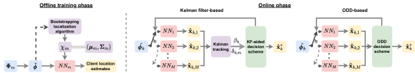
Fig. 1 illustrates the workflow of our proposed localization scheme, which consists of two phases. In the offline training phase, NN (corresponding to section of a large indoor space) is trained using the ADoA values computed from the AoA measurements (obtained by processing channel state information (CSI) at the client as in [9, 14]). These are fed to the bootstrapping localization algorithm to obtain training labels and their corresponding mean-covariance matrix pair (. These labels are used to train NN . Note that the input to both our NN model and the bootstrapping localization algorithm are the same, i.e, .
For the online training phase, we propose two schemes. The first scheme exploits the location estimates from the NN to track the evolution of the client’s state. We exploit the state innovation and the normalized innovation squared (NIS) metric of the predicted state, which measures how accurately the Kalman filter predicted the measurements, to choose the best NN. The second scheme exploits the statistical parameters of the training labels to compute the distance between the NN estimates from different training label distributions. The idea is to compute the distance between the NNs’ estimates and the distribution of the labels (in this work, we resort to the Mahalanobis distance). As the wrongly estimated location will be far from the distribution corresponding to the true label, we refer to this scheme as out-of-distribution detection.
III-B Kalman filter (KF)-based decision scheme
The KF-based scheme involves two stages: the trajectory tracking phase and the decision phase.
Kalman tracking phase. In this phase, we track the evolution of the client trajectory, as estimated by our trained NNs, using a Kalman filter [15]. Let the state of the client at time be , where and are the 2-D coordinates of the client, and and are the and component of it’s velocity. The state evolves in time following a constant-velocity (CV) model. The evolution of the state at is given as , where is the state transition matrix that transforms the state of the client at time step to , and represents the zero-mean Gaussian distributed process noise with covariance matrix . Here, s, is the Kronecker product, and is the identity matrix. The predicted state representing the 2D location of the client is , where is the observation matrix given by diag and is the zero mean Gaussian observation noise, with the observation noise covariance matrix .
The Kalman filter performs two steps: prediction and model update. The prediction step estimates the current a priori state of the client based on the previous a posteriori estimate , i.e., , and also computes the a priori state covariance matrix . The model update equations correct the existing state predictions and the covariance matrix using the measurement vector and the updated Kalman gain. The prediction error is the innovation of the Kalman filter and is given as
| (1) |
This is used to correct the predicted state of the client as , where is the Kalman gain.
We exploit the innovation along with the innovation covariance , to compute
| (2) |
We also compute the Euclidean distance between the predicted state and the current measurement , given as . We use and to implement the decision scheme to switch among the NNs.
KF-based decision scheme. The measurements used by the Kalman filter are the location estimates obtained from NN , i.e., the NN model trained in section of the indoor space. NN will be able to estimate the client location accurately, as long as the client is moving within region . Thus, a Kalman filter will be able to predict the location of the client with a low . At any time step , as the client moves into another region, NN will be unable to estimate the location of the client accurately. This is because the client will not be able to listen to all the multipath components from the APs of the previous region. However, the Kalman filter would predict the location estimate based on the model learned up to time step , thus the Kalman predicted state would be closer to the location of the client. As the current NN will be unable to accurately localize the client, this would result in a large and an even larger . When exceeds a user-defined threshold , we feed the corresponding ADoA measurements to the trained NN models to compute the location estimate , where . We select the NN that minimizes the Euclidean distance between and the Kalman-predicted location :
| (3) |
where , with the best estimate of the client being . The subsequent set of measurements for the Kalman filter would be the locations estimated by NN . We repeat this procedure to switch to the right NN whenever the metric exceeds a threshold . In our evaluation, we set . This aligns with the theoretical result that the expectation of should equal the number of degrees of freedom of the Kalman filter (i.e., the 2 coordinates of the client in our case) [16].
III-C Out-of-distribution detection (ODD) switching scheme
In this approach, we exploit the statistical properties of the location labels used to train the NNs of each section of the indoor space. Specifically, we compute the mean and the covariance of the training labels distribution corresponding to region obtained from the offline training phase. Each distribution is characterized by its mean-covariance pair . In the online testing phase, at any time instance , if the distance between the current location estimate and the previous estimate exceeds a user-defined threshold , i.e., , where is the distance threshold (1 m in our case), the ADoA values at test location are fed to NNs. This results in location estimates . We then compute the Mahalanobis distance of from each of the distributions as
| (4) |
The Mahalanobis distance measures the distance of a point from a distribution of points, where, the smaller the distance, the closer the point to the distribution. We finally choose the best NN as , and its corresponding estimate as the best location estimate. Whenever the location estimated by NN is far from the previous estimate, i.e., the Euclidean distance between the current estimate and the previous estimate exceeds the distance threshold (chosen after exhaustive search), we repeat the above procedure and switch to another NN model.
III-D Tiny neural network architecture
We resort to a 4-layer tiny NN model with neurons in each layer. Here, is greater than or equal to the number of ADoAs from visible anchors [5], , , , and represents the ceiling function. The NN has two output neurons, corresponding to the 2D coordinates of the client. The NN learns a non-linear regression function between the ADoAs and the client location . The regression problem is framed to minimize the mean-square error (MSE) between the self-supervised training labels and the locations estimates obtained from the NN. The NN employs the rectified linear unit (ReLU) activation function and Adam optimizer. The hyperparameters used for tuning the NN to minimize the loss function are the factor , dropout rate , learning rate , and the training batch size .
IV Simulation Results
IV-A Simulation environment
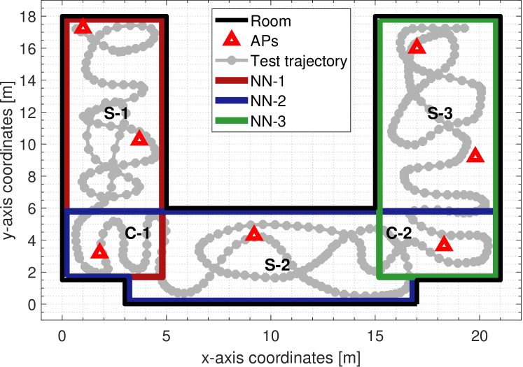
We validate the performance of our proposed schemes via a simulation campaign. We simulate human motion trajectories in an irregular U-shaped room as shown in Fig. 2, comprising two vertical rectangular sections (S-1 and S-3) of size 5 m 18 m and 6 m 18 m, connected by a 20 m wide horizontal section (S-2). We deploy seven mmWave APs to cover the indoor space. We collect AoAs from all the APs and their corresponding virtual anchors (VAs) (mirror images of the physical APs with respect to each wall of the room) at each client location along a trajectory using a ray tracer. To simulate realistic noisy measurements, we perturb the AoAs with zero-mean Gaussian noise of standard deviation .
We train each model with locations within each boxed section (S-1, S-2, S-3) in Fig. 2. The trained NNs have the following architecture: NN-1 and NN-2 have neurons in each layer with , , , , and , , , respectively, while NN-3 has neurons with , , , . We test the trained NNs on a trajectory comprising 388 client locations across the three sections of the room (grey line).
IV-B Analysis of the switching schemes
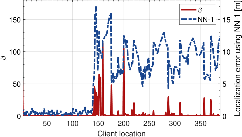
We first analyze the performance of the KF-based switching scheme. Fig. 3 illustrates the metric computed while using NN-1 to track the client along the test trajectory. The figure also presents the localization error when using NN-1. Initially, when NN-1 estimates the client locations in S-1, is close to zero. As the client crosses the border of S-1 and S-2 (around location 140), the errors of NN-1’s estimates increase. These estimates significantly deviate from the client’s state as predicted by the Kalman filter, resulting in a large and hence an even larger value, leading to the appearance of peaks. Conversely, with every subsequent wrong estimates by NN-1, the Kalman filter keeps predicting the client’s location to be around the wrong estimates, resulting again in low values of . This trend can be observed when the client moves in S-2 and S-3.
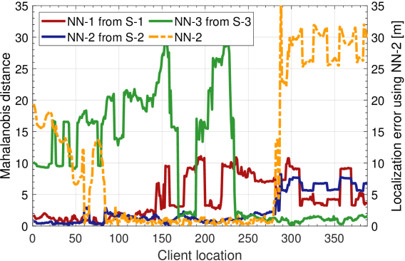
We now analyze the ODD scheme. Fig. 4 illustrates the Mahalanobis distance between the location estimates obtained from different NNs and the distribution of the training data corresponding to each section of the room, as a function of the client location. The locations estimated by the NNs and lying within the distribution of the training data consistently yield . We also observe that a large set of locations in the common sections of the room, i.e., C-1 (client locations from 90 to 140) and C-2 (from 235 to 270), were localized accurately by the NNs sharing the overlapped regions, as they compute the ADoAs from the same set of visible anchors. Thus, these estimates have similar values, as they are part of two s. In such situations, we can exploit the Euclidean distance between the current location estimate and the previous location estimate to choose the right NN.
While the values of for NN-1 and NN-3 are low in their respective regions and easily distinguishable thanks to ADoA measurements from a disjoint set of APs, the values for location estimates from NN-2 are low for the entire trajectory. This is because a vast majority of the locations in S-2 can compute the ADoA values from multipath components (MPCs) arriving from all the APs. Thus, NN-2 estimates the client locations closer to all the three s. However, the localization error (yellow dashed line) is still large, especially for the locations in the non-overlapping regions of S-1 and S-3. This implies that NN-2’s location estimates, even though highly erroneous, lie within the other two distributions. Thus, we remark that the ODD technique is more appropriate in environments where each section is illuminated by a disjoint set of APs.
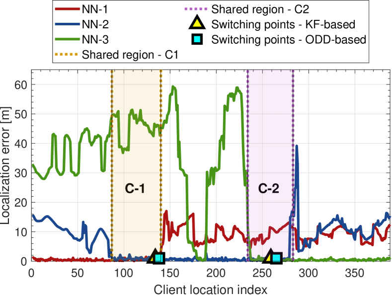
The switching points obtained from the KF-based (triangles) and ODD-based (squares) switching schemes are depicted in Fig. 5. The dotted and shaded sections are the borders and the common areas C-1 and C-2, between the S-1 and S-2, and S-2 and S-3 respectively. The ideal switching points are within the boundaries of C-1 and C-2 (see Fig. 2), from location index 90 to 140 (C-1) and from 235 to 270 (C-2). We observe that both schemes decide to switch NN models within the ideal switching area. However, unlike the ODD scheme, the KF-based scheme tends to be more robust, as it uses the motion model of the client to predict its future location.
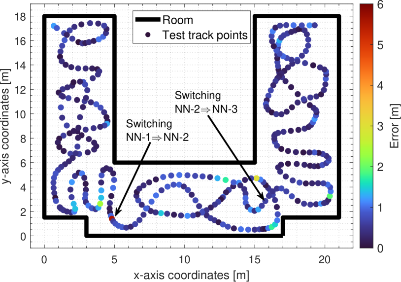
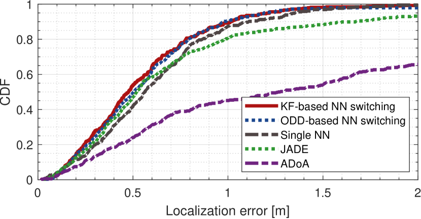
Fig. 6 illustrates the localization errors at each location along the test track, where we consider the NN switching points obtained from the KF-based scheme, and concatenate the location estimates of each NN. Here, blue hues represent errors m whereas green to red hues correspond to higher errors. We observe sub-meter errors at most locations, and slightly larger errors near the bottom left and right corners, and at the switching points, where the NN being used cannot accurately localize the client. Fig. 7 presents the cumulative distribution function (CDF) of the localization errors of the reconstructed trajectory and of the trajectory estimated using the JADE algorithm, a single self-supervised NN, and the geometric ADoA algorithm [8]. We observe that JADE and our self-supervised NNs outperform the ADoA scheme [5]. While JADE achieves sub-meter localization errors in 80% of the cases (mean error of 0.74 m), a single NN performs better with sub-meter errors in about 87% of the cases (mean error of 0.63 m). Likewise, choosing the right NN via the KF- or ODD-based schemes achieves sub-meter errors in about 90% of the cases. We note that running JADE on the entire trajectory results in large errors, especially when moving closer to the bottom left and right corners of the room. This is because noisy ADoA values largely offset the estimates of the associated anchors. Moreover, using a single NN instead of multiple NNs results in large training and bootstrapping algorithm complexity, and a single NN typically needs additional hidden layers to accurately localize a client in complex-shaped environments. Thus, training a different, smaller NNs (each for a different portion of the environment) and employing our proposed switching schemes can help accurately localize a client in large or irregular rooms.
V Conclusions
In this letter, we proposed to employ multiple self-supervised tiny NN models to accurately localize a client as it moves across a large indoor environment. We presented two schemes based on innovation of Kalman filters and statistical distribution of training labels, to dynamically choose the best NN model to accurately localize a client. Results show that the trajectory reconstructed upon switching to the right NNs using the proposed schemes achieves 1 m localization error in 90% of the cases. We can conclude that both schemes can aid to dynamically switch to the best NN. However, the KF-based scheme is more robust, owing to its ability to track client’s motion, thus predicting its trajectory using NN estimates. In contrast, the ODD scheme could be a feasible choice in large distributed environments, where different sections of the indoor space are illuminated by a disjoint set of APs.
References
- [1] A. Shastri, N. Valecha et al., “A review of millimeter wave device-based localization and device-free sensing technologies and applications,” IEEE Commun. Surveys Tuts., vol. 24, no. 3, pp. 1708–1749, 2022.
- [2] I. A. Hemadeh, K. Satyanarayana et al., “Millimeter-wave communications: Physical channel models, design considerations, antenna constructions, and link-budget,” IEEE Commun. Surveys Tuts., vol. 20, no. 2, pp. 870–913, 2018.
- [3] C. Fiandrino, H. Assasa et al., “Scaling millimeter-wave networks to dense deployments and dynamic environments,” Proc. IEEE, vol. 107, no. 4, pp. 732–745, 2019.
- [4] T. Koike-Akino, P. Wang et al., “Fingerprinting-based indoor localization with commercial mmWave WiFi: A deep learning approach,” IEEE Access, vol. 8, pp. 84 879–84 892, 2020.
- [5] A. Shastri, J. Palacios, and P. Casari, “Millimeter wave localization with imperfect training data using shallow neural networks,” in Proc. IEEE WCNC, 2022, pp. 674–679.
- [6] J. Palacios, P. Casari, and J. Widmer, “JADE: Zero-knowledge device localization and environment mapping for millimeter wave systems,” in Proc. IEEE INFOCOM, 2017, pp. 1–9.
- [7] F. Zafari, A. Gkelias, and K. K. Leung, “A survey of indoor localization systems and technologies,” IEEE Commun. Surveys Tuts., vol. 21, no. 3, pp. 2568–2599, 2019.
- [8] J. Palacios, G. Bielsa et al., “Single-and multiple-access point indoor localization for millimeter-wave networks,” IEEE Trans. Wireless Commun., vol. 18, no. 3, pp. 1927–1942, 2019.
- [9] A. Blanco, P. J. Mateo et al., “Augmenting mmWave localization accuracy through sub-6 GHz on off-the-shelf devices,” in Proc. ACM Mobisys, 2022, p. 477–490.
- [10] D. Garcia, J. O. Lacruz et al., “POLAR: Passive object localization with IEEE 802.11ad using phased antenna arrays,” in Proc. IEEE INFOCOM, 2020, pp. 1838–1847.
- [11] P. Wang, M. Pajovic et al., “Fingerprinting-based indoor localization with commercial mmWave WiFi - Part II: Spatial beam SNRs,” in Proc. IEEE GLOBECOM, 2019, pp. 1–6.
- [12] C. J. Vaca-Rubio, P. Wang et al., “mmWave Wi-Fi trajectory estimation with continuous-time neural dynamic learning,” in Proc. IEEE ICASSP, 2023, pp. 1–5.
- [13] A. Vashist, M. P. Li et al., “KF-Loc: A Kalman filter and machine learning integrated localization system using consumer-grade millimeter-wave hardware,” IEEE Consum. Electron. Mag., vol. 11, pp. 65–77, 2022.
- [14] Y. Xie, J. Xiong et al., “MD-Track: Leveraging multi-dimensionality for passive indoor Wi-Fi tracking,” in Proc. ACM MobiCom, Aug. 2019.
- [15] R. E. Kalman, “A new approach to linear filtering and prediction problems,” 1960.
- [16] I. Reid and H. Term, “Estimation II,” University of Oxford, Lecture Notes, 2001.