JADES: A large population of obscured, narrow line AGN at high redshift

We present the identification of 42 narrow-line active galactic nuclei (type-2 AGN) candidates in the two deepest observations of the JADES spectroscopic survey with JWST/NIRSpec. The spectral coverage and the depth of our observations allow us to select narrow-line AGNs based on both rest-frame optical and UV emission lines up to z=10. Due to the metallicity decrease of galaxies, at $z>3$ the standard optical diagnostic diagrams (N2-BPT or S2-VO87) become unable to distinguish many AGN from other sources of photoionisation. Therefore, we also use high ionisation lines, such as He ii $\lambda$4686, He ii $\lambda$1640, [Ne iv] $\lambda$2422, [Ne v] $\lambda$3420, and N V $\lambda$1240, also in combination with other UV transitions, to trace the presence of AGN. Out of a parent sample of 209 galaxies, we identify 42 type-2 AGN (although 10 of them are tentative), giving a fraction of galaxies in JADES hosting type-2 AGN of about $20\pm 3$%, which does not evolve significantly in the redshift range between 2 and 10. The selected type-2 AGN have estimated bolometric luminosities of $10^{41.3-44.9}$ erg s^-1 and host-galaxy stellar masses of $10^{7.2-9.3}$ M_⊙. The star formation rates of the selected AGN host galaxies are consistent with those of the star-forming main sequence. The AGN host galaxies at z=4-6 contribute $\sim$8-30 % to the UV luminosity function, slightly increasing with UV luminosity.

1 Introduction

It has been widely accepted that supermassive black holes (SMBHs) reside in the centre of most (perhaps all) massive galaxies. During their accretion phases, SMBHs are observed as active galactic nuclei (AGN; Rees et al., 1982; Lynden-Bell, 1969; Soltan, 1982; Merloni et al., 2004). The tight correlation between a SMBH mass and host-galaxy bulge properties (such as velocity dispersion and mass) at $z\sim 0$ indicates a strong connection between the growth of a SMBH and its host galaxy (e.g., Magorrian et al., 1998; Kormendy & Ho, 2013). Furthermore, (radiative and mechanical) feedback from AGNs is a key ingredient of galaxy evolution, as AGNs can inject a significant amount of energy into the interstellar and circumgalactic medium (ISM and CGM, respectively) of their host galaxies. AGN feedback is necessary to reproduce key galaxy properties such as: colour bi-modality, galaxy sizes, and a broader range of specific star formation rates and enrichment of the intergalactic medium (IGM) by metals, as well as the high-mass drop-off of the stellar mass function compared to the halo mass function (e.g., Silk & Rees, 1998; Di Matteo et al., 2005; Alexander & Hickox, 2012; Dubois et al., 2013b, a; Vogelsberger et al., 2014; Hirschmann et al., 2014; Crain et al., 2015; Segers et al., 2016; Beckmann et al., 2017; Harrison, 2017; Choi et al., 2018; Scholtz et al., 2018).

The identification and study of AGN at high redshift is essential to understanding not only the co-evolution of SMBHs and galaxies, but also the formation of galaxies at early epochs. Although over the past 15 years there has been significant progress in the identification of active SMBHs at high redshift ($z>3$) (e.g. Merloni et al., 2010; Bongiorno et al., 2014; Trakhtenbrot et al., 2017; Mezcua et al., 2018; Lyu et al., 2022), the majority of these detections have been limited to bright quasars identified in large-volume ground-based surveys (e.g., Bañados et al. 2016; Shen et al. 2019, see Inayoshi et al. 2020; Fan et al. 2022 for a review). These include the most distant identified quasars at $z\sim 7.5$ (Bañados et al., 2018; Yang et al., 2020; Wang et al., 2021).

With the launch of the James Webb Space Telescope (JWST; Gardner et al., 2023; Rigby et al., 2023), we now have access to rest-frame UV-to-optical emission lines of galaxies up to $z\sim 12$. These lines allow us to identify and study AGNs, even at low masses and luminosities, via optical and UV diagnostic diagrams. A number of AGN candidates have already been identified by performing Spectral Energy Distribution (SED) analyses of broad-band photometry from NIRCam and MIRI aboard JWST (Furtak et al., 2022; Onoue et al., 2023; Barro et al., 2023; Yang et al., 2023a; Bogdan et al., 2023; Juodžbalis et al., 2023; Lyu et al., 2023; Yang et al., 2023b). Significant progress has been made using deep spectroscopy from JWST/NIRSpec (Böker et al., 2022; Jakobsen et al., 2022) and the JWST/NIRCam grism, tracing the presence of a broad line region (BLR; Furtak et al., 2023; Greene et al., 2023; Harikane et al., 2023; Kocevski et al., 2023; Maiolino et al., 2023b, a; Matthee et al., 2023; Onoue et al., 2023; Übler et al., 2023). These observations revealed a previously unseen population of AGN at z$>4$, and out to z$\sim$11, with estimated black hole masses (M_BH) in the range $\rm 10^{6}$ to $\rm 10^{8}\leavevmode\nobreak\ M_{\odot}$ and bolometric luminosities $\rm 10^{44}-10^{45}\leavevmode\nobreak\ erg\leavevmode\nobreak\ s^{-1}$. These black hole masses and luminosities are 2–3 orders of magnitude lower than those inferred for quasars at the same redshifts (Mazzucchelli et al., 2023; Zappacosta et al., 2023).

However, identification of narrow-line (i.e. type-2, as opposed to type-1 AGN showing BLR emission) AGN has remained unexplored with JWST data. This has been the main AGN identification tool at low redshift, however, so far has had limited success at high redshift. The reason is most likely the rapid evolution of the metallicity and ionisation parameter at z¿3 towards more metal poor and higher ionisation parameter (Hirschmann et al., 2022; Curti et al., 2023b, a; Tacchella et al., 2023; Trump et al., 2023). Indeed, Harikane et al. (2023); Kocevski et al. (2023); Maiolino et al. (2023a); Übler et al. (2023) have shown that the type-1 AGN found by JWST have narrow line ratios on the classical emission-line diagnostic diagrams (such as BPT; Baldwin et al. 1981a; Kauffmann et al. 2003; Kewley et al. 2013 and VO87; Veilleux & Osterbrock 1987) that overlap with the local SF sequence, and not with the region occupied by nearby and low-z AGN. This displacement has been predicted by photoionization models for low metallicity AGN (Groves et al., 2006; Nakajima & Maiolino, 2022). Additionally, Feltre et al. (2016) and Gutkin et al. (2016) ran photo-ionisation grid models to assess the effect of low metallicity and high ionisation parameter on rest-frame optical and UV emission lines, and found that the nebular emission of star-forming galaxies at high redshift become similar to that of AGN, further complicating the AGN selection via narrow emission line diagnostics. The identification of type-2 AGN at high redshift can still rely on high ionization lines, such as the [Ne iv] $\lambda$2424 (with ionisation potential $>$63.45eV) detected by Brinchmann (2023) in a galaxy at z = 7.66. Luckily, the identification of type-2 AGN with high metallicity through standard BPTs is still possible (see Perna et al. 2023)

Despite these newly discovered AGN being far less luminous than the previously known quasar population and being hosted in galaxies with lower masses, they can play a major role in shaping galaxy evolution (via positive and negative feedback; Koudmani et al., 2021, 2022) and could potentially significantly contribute to the reionisation of the Universe. Indeed, we have already observed these processes in GN-z11 (Bunker et al., 2023b) believed to host an AGN (Maiolino et al., 2023b) with detected outflow in the system, while Scholtz et al. (2023) observed heating and ionisation of the circum-galactic medium around this unique galaxy. These examples show the presence of AGN feedback at high z, which can explain the early emergence of quiescent galaxies and high burstiness of star formation (Carnall et al., 2023b, a; Endsley et al., 2023; Looser et al., 2023c, a; Dome et al., 2023; Strait et al., 2023); indeed, Gelli et al. (2023) showed that supernovae feedback is not sufficient to rapidly suppress the star formation in some of these rapidly quenched systems.

In this paper, we leverage two of the deepest spectroscopic observations from JWST Advanced Deep Extragalactic Survey (JADES, Proposal ID: 1210 & 3215; Bunker et al. 2023a; Curtis-Lake et al. 2023; Eisenstein et al. 2023b, a; Robertson et al. 2023). Using this deep spectroscopy with JWST/NIRSpec, we aim to identify type-2 AGN using deep spectroscopy with JWST/NIRSpec in galaxies with stellar masses M${}_{*}\sim 10^{6.5}-10^{9.5}$ M_⊙ from redshift z = 1 and out to the highest redshifts for which rest-frame UV and optical nebular lines are accessible to NIRSpec (z$\sim$12.0). We reassess the demarcation lines between AGN and star-forming galaxies at high redshift and further refine selection criteria using the photo-ionisation modelling introduced by Feltre et al. (2016) and Nakajima & Maiolino (2022).

The paper is organized as follows. In Section 2, we describe the observations, data reduction, spectral fitting procedures, and SED analysis to derive stellar masses and star formation rates (SFRs). In Section 3 we identify AGN using their narrow line properties of rest-frame UV and optical emission lines. In Section 4, we estimate the properties of the AGN and their host galaxies and discuss our results. In Section 5, we draw our conclusions. Throughout this paper, we use the AB magnitude system and assume a flat $\Lambda$CDM cosmology with $\Omega$m = 0.315 and H₀ = 67.4 km/s/Mpc Planck Collaboration et al. (2020) cosmology and a Chabrier (2003) initial mass function.

2 Observations, Data reduction and Analysis

The observations of our targets were obtained as part of the JADES survey, utilising the multi-object spectroscopic capabilities of the JWST/NIRSpec micro-shutter array (MSA; Jakobsen et al. 2022; Ferruit et al. 2022) across two programmes: PID 1210 & PID 3215.

Five disperser/filter combinations were used: the low-resolution PRISM/CLEAR ($0.6<\lambda<5.3\leavevmode\nobreak\ \mu$m$,R=30-300$; Jakobsen et al., 2022), the medium-resolution gratings G140M/F070LP, G235M/F170LP and G395M/F290LP ($0.6<\lambda<5.3\leavevmode\nobreak\ \mu$m, $R=1,000$), and the high-resolution grating G395H/F290LP ($2.8<\lambda<5.1\leavevmode\nobreak\ \mu$m, R=2,700). For the 1210 program, the observations consist of individual visits with a per-visit duration of 33.6 ks for the prism, and of 8.4 ks for each grating. Each galaxy was assigned a minimum of one and a maximum of three visits depending on its priority (Bunker et al., 2023a). This resulted in a maximum integration time of $\sim 100$ ks for the prism and of 25 ks for each grating. The 3215 program consisted only of three configurations: PRISM/CLEAR, G140M/F070LP, and G395M/F290LP, with a maximum resulting integration time of 168 ks, 42 ks, and 168 ks.

The observations were performed in the three-shutter nod mode, so that common targets were observed in different shutters and different locations on the detector. Therefore, each visit required a unique MSA configuration. Each target allocation (performed using the eMPT tool; Bonaventura et al. 2023) was designed to maximise the number of targets that have all the disperses/filters in common between all the dither positions, however, not all targets have the full on source integration time outlined above. In total, we observed 481 unique targets.

The MSA configurations have been designed to avoid spectral overlap for the prism mode. However, since the spectra taken with the medium or high-resolution gratings occupy a significantly larger portion of the detector, and to avoid removing targets with overlapping spectra, we allowed spectral overlap for these modes. The MSA configurations were, however, designed to minimize the negative effect of spectral overlap on our science, since the highest priority targets are not allowed to be contaminated by neighboring spectra. We show examples of the acquired PRISM/CLEAR spectra in Figure 1.

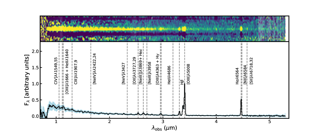
Figure 1: Example of low-resolution PRISM/CLEAR spectrum of galaxy (JADES-NS-GS-00022251) at z = 5.804 included in our parent sample. The spectrum is shown in units of F_λ normalized to the [O iii] $\lambda$5008 peak. We highlight major emission lines used in our analysis.

2.1 Data Reduction

The JWST/NIRSpec MSA observations were processed with the data reduction pipeline of the ESA NIRSpec Science Operations Team (SOT) and the NIRSpec GTO Team, further detailed description of the GTO pipeline will be presented in Carniani et al. (in prep), and is summarised in Bunker et al. (2023a). Here, we briefly summarize the procedure. We retrieve the level-1a data products from the MAST archive and estimate the count-rate slopes per pixel, using the unsaturated groups in the ramps. We remove any jumps in the ramps due to cosmic rays by estimating the slope of each ramp. During this stage, we perform the master dark and bias subtraction, as well as the flagging of saturated pixels. The background subtraction is performed pixel by pixel by combining the three nod exposures of each pointing. We note that for some targets we excluded one of the 3-shutter nods in the background subtraction stage as a serendipitous source contaminated the open shutters. We performed the flat-field correction of the spectrograph optics and disperser corrections on the 2D-dimensional cutouts of each of the three-shutter slits. The path loss corrections are calculated assuming point sources and taking into account the source location on the shutter.

Finally, the individual 2D maps are interpolated onto an irregular wavelength grid for the PRISM/CLEAR observations (to avoid oversampling the line spread function below 2 $\mu$m) and onto a regular grid for the gratings. We extracted the 1D spectra from the 2D maps adopting a box-car aperture centered on the relative position of the targets. We combined all 1D spectra and removed the bad pixels by adopting a sigma-clipping approach.

2.2 Spectral fitting using PPXF

As the continuum is well detected in all our targets in the PRISM observations, we employed pPXF (Cappellari, 2017, 2022) to fit the continuum and emission lines simultaneously. As we are interested in inactive galaxies or type-2 AGN, there is no contamination of the continuum by the AGN, making pPXF an ideal tool for this analysis. The continuum is fitted as a linear superposition of simple stellar-population (SSP) spectra, using non-negative weights and matching the spectral resolution of the observed spectrum. As input stellar templates we used the synthetic library of simple stellar population spectra (SSP) from fsps (Conroy et al., 2009; Conroy & Gunn, 2010). This library uses MIST isochrones (Choi et al., 2016) and C3K model atmospheres (Conroy et al., 2019). We also used fit a 5^th-order multiplicative polynomial, to capture the combined effects of dust reddening, residual flux calibration issues, and any systematic mismatch between the data and the input stellar templates. We find that the NIRSpec/MSA data are fit adequately by low-order polynomials. Increasing the polynomial degree does not improve the fit results (as quantified by the value of the reduced $\chi^{2}$). To simplify the fitting, any flux with a wavelength shorter than Lyman break is manually set to 0. The full description of the pPXF fitting will be presented in D’Eugenio et al. (in prep).

For the emission lines fitting we use the redshifts published in the Bunker et al. (2023a), which used redshifts determined from the medium resolution gratings available and PRISM spectra otherwise. All emission lines are modeled as single Gaussian functions, matching the observed spectral resolution. We use vacuum wavelengths for the emission lines throughout the paper. In order to remove degeneracies in the fitting and reduce the number of free parameters, the emission lines are split into four separate kinematic groups, bound to the same redshift and intrinsic broadening. These groups are as follows:

• UV lines with rest-frame $\lambda<3000$ Å.

• The hydrogen Balmer series.

• Non-hydrogen optical lines with rest-frame $\lambda<9000$ Å.

• Near infra-red lines.

The stellar kinematics are tied to the Balmer line kinematics. For emission line multiplets arising from the same level, we fixed the emission line ratio to the value prescribed by atomic physics (e.g., [O iii] $\lambda$5008/[O iii] $\lambda$4959 = 2.99). For multiplets arising from different levels, the emission line ratio can vary. This is relevant for five multiplets: C iv $\lambda\lambda$ 1548,1551, C iii] $\lambda\lambda$1907,1909, [O ii] $\lambda\lambda$3727,3730 and [S ii] $\lambda\lambda$6718,6733. However, in practice, the spectral resolution of the PRISM/CLEAR observations is insufficient to resolve the individual lines in each multiplet. For this reason, we model each of these as a single Gaussian in the PRISM observations. In addition, as the He ii $\lambda$1640 and [O iii] $\lambda$$\lambda$1661,66 are blended together we are unable to use their measured fluxes from the PRISM observations and instead, choose to use the R1000 observations. The fits are performed in two steps. In the first run, we tie the kinematics as described above, and identify robust detections (above 5-$\sigma$ significance) for re-fitting. In the second run, we only fit for these detected lines, but allow for their kinematics to vary independently from one another.

The R1000 gratings were fitted using the same procedure as for the PRISM observations, by combining all three gratings and fitting them simultaneously. However, we did not stack the spectra from different gratings, because this would combine the highest-resolution end of one grating with the poorest-resolution start of the next grating.

2.2.1 Fitting the UV lines

The high ionisation UV lines were excluded from the pPXF fitting as they are extremely faint and blended in the PRISM data. Since the AGN high ionisation UV lines are considerably fainter than the optical emission lines, we fitted only objects that are well-detected in [OIII] or H$\alpha$ emission (SNR$>10$).

We fitted the [Ne iv] $\lambda$2424, [Ne v] $\lambda$3420 and N V $\lambda$1240 using QubeSpec’s fitting module. Each emission line was fitted using a single Gaussian component and the continuum was fitted as a power law. This simplistic approach is sufficient for describing a narrow range of the continuum around an emission line of interest. As QubeSpec is a Bayesian code implemented using emcee (Goodman & Weare, 2010), it is necessary to also supply priors on each quantity. The peak of the Gaussian and continuum normalization are given a log-uniform prior, while the FWHMs are set to a uniform distribution spanning from the minimum resolution of the NIRSpec/MSA ($\sim$200 kms^-1) up to a maximum of 1200 km/s. The prior on the redshift was a normal distribution centered on the redshift obtained from pPXF with a standard deviation of 300 km/s. This is done because as the high ionisation UV lines originate from close to the accretion disc, there can be a significant velocity offset between the low and high ionisation lines in an AGN. We report the fluxes of each of these high ionisation lines in the Appendix in Table 5. Throughout this work we derived upper limits as 3$\sigma$.

2.3 SED fitting using BEAGLE

In order to compare our selected AGN with the rest of the galaxy population, it is necessary to measure the stellar masses and star-formation rates of our sample. We use the full fitting of the slit-loss corrected PRISM spectra using the BEAGLE tool (Chevallard & Charlot, 2016). We assume a delayed-exponential star-formation history (SFH), while decoupling the current SFR from the previous SFH by allowing a recent duration of 10Myr of constant star formation to vary independently. A Chabrier (2003) initial mass function (IMF) with an upper mass cut-off of 100 M_⊙ was adopted using the updated Bruzual & Charlot (2003) stellar population models described in Vidal-García et al. (2017a). We define the total stellar mass as the mass currently locked into stars. This definition accounts for the fraction of mass returned to the ISM during stellar evolution. The SFRs of our objects are averaged over 10 million years.

We note that the SFRs of the whole sample estimated with BEAGLE are in excellent agreement with those estimated from the dust-corrected Balmer lines (H$\alpha$ and H$\beta$; see Curti et al. 2023b for more information).

2.4 Comparison to photoioinization models

At high redshifts, galaxies become more metal-poor and show an increasingly higher ionisation parameter (see Hirschmann et al., 2022; Schaerer et al., 2022; Cameron et al., 2023b; Curti et al., 2023b; Trump et al., 2023), resulting in standard diagnostics diagrams used to identify AGNs at low redshift becoming less useful (see Kewley et al., 2013, 2019; Hirschmann et al., 2022). We, therefore, consider the photoionisation models initially described in Feltre et al. (2016) and Gutkin et al. (2016), and updated with more recent stellar spectra and with a better description of AGN cloud microturbulence (Vidal-García et al., 2017b; Mignoli et al., 2019; Hirschmann et al., 2019). These works consider a large grid of photoionisation models computed using the CLOUDY code (Ferland et al., 2013) for star formation and AGN narrow-line regions, and for various gas metallicities, dust content, and ISM densities. From these model grids, we selected all models with metallicities between 0.001 and 0.02 (corresponding to 0.06-1.3 solar) and a dust-to-metal mass ratio of 0.3. This value is intermediate between the range observed in the most metal-poor absorbers (e.g., Konstantopoulou et al., 2023) and the Milky-Way value of 0.45. We consider all models with carbon-to-oxygen abundance ratio in the range 0.38-1.00 solar to describe a variety of different or less common star-formation grids. We further restrict the grids to only include models with an IMF upper mass cut-off of 300 M_⊙, similar to the SED fitting above.

We also compare our observed emission line ratios with the models of Nakajima & Maiolino (2022). They investigated the emission line ratios of star-forming galaxies, AGN, PopIII stars, and Direct Collapse black holes (DCBHs) using the Cloudy code and the BPASS stellar population models (Eldridge et al., 2017). In this work, we only use the models for star-forming galaxies and AGN host galaxies, as our objects do not have low enough metallicities to host either PopIII or DCBHs (based on values from Curti et al., 2023b). We selected the same metallicities, dust-to-metal mass ratio and IMF upper cutoff as for the Gutkin et al. (2016) and Feltre et al. (2016) models.

Throughout this work, we present these models on our diagnostics plots (Figures 2, 3, 4 and 6) as light blue and yellow circles for AGN and star-formation, respectively. We will further discuss these points and use them to redefine the selection of AGN based on to-be-introduced N2-BPT and S2-VO87 diagnostic diagrams in §3.1.

3 Selection of AGN in JADES deep spectroscopic data

In order to select AGN based on their narrow line properties we require a 3$\sigma$ detection of the following lines: H$\alpha$, H$\beta$, [O iii] and C iii], and wavelength coverage of [S ii], [N ii] and UV and optical He ii  and C iv  for the optical and UV line selection. Overall, this yields a sample size of 110 and 99 sources for the programmes 1210 and 3215, respectively. We define the line ratios used in this paper in Table 1 (see below) and we summarise all emission lines, their wavelengths and ionisation potential in the Appendix in Table 6. We consider a galaxy an AGN candidate if it appears as an AGN in at least one diagnostic. Furthermore, we report the list of selected AGN candidates, field, coordinates, redshift, the method with which we detect it, and other notes in Table 2.

Table 1: Definitions of line ratios adopted throughout the paper.

Diagnostics	Line Ratio
R3	[O III]$\lambda$5008 / H$\beta$
N2	[N II]$\lambda$6584 / H$\alpha$
S2	[S II]$\lambda\lambda$6718,32 / H$\alpha$
Ne3O2	[Ne III]$\lambda$3869 / [O II]$\lambda\lambda$3727,29
He2	He II$\lambda$4686 / H$\beta$
C43	C IV$\lambda\lambda$1549,51/C III]$\lambda\lambda$1906,08
C3He2	C iii]$\lambda\lambda$1906,08 / He II$\lambda$1640
Ne4C3	[Ne iv] $\lambda$$\lambda$2422,24/C III]$\lambda\lambda$1906,08
Ne5C3	[Ne v] $\lambda$$\lambda$3427,29/C III]$\lambda\lambda$1906,08
N5C3	N V $\lambda$$\lambda$1239,42/C III]$\lambda\lambda$1906,08

Table 2: List of AGN from JADES HST Deep selected in this work. Columns: ID, redshift, detection method, stellar mass, SFR and UV magnitude from BEAGLE, AGN bolometric luminosity and any other additional notes. We note that for bolometric luminosity the uncertainties are dominated by the systematical uncertainties (0.3-0.5 dex).

ID	field	z	selection	log10 M∗	SFR	MUV	log10 Lbol	Notes
			method	M⊙	M⊙ yr-1		ergs s-1
JADES-NS-GS00004902	1210	5.123	S2-VO87*	8.6${}^{0.03}_{0.02}$	1.4${}^{0.21}_{-0.14}$	-19.0	43.0
JADES-NS-GS00007099	1210	2.860	S2-VO87*	9.1${}^{0.01}_{0.01}$	1.1${}^{0.07}_{-0.06}$	-17.4	42.9
JADES-NS-GS00007762	1210	4.146	High ion	8.2${}^{0.02}_{0.02}$	4.1${}^{0.29}_{-0.28}$	-18.8	43.6	outflows
JADES-NS-GS00008083	1210	4.665	High ion & HeII$\lambda 4686$	7.8${}^{0.01}_{0.01}$	7.3${}^{0.12}_{-0.12}$	-18.5	44.5	Type-1 & LAE
JADES-NS-GS00008456	1210	1.884	HeII$\lambda 4686$	8.1${}^{0.03}_{0.08}$	0.1${}^{0.03}_{-0.01}$	-16.1	41.6
JADES-NS-GS00008880	1210	2.327	N2-BPT	7.1${}^{0.25}_{0.70}$	0.1${}^{0.03}_{-0.02}$	-14.9	42.0
JADES-NS-GS00009422	1210	5.942	HeII$\lambda 1640$ & HeII$\lambda 4686$	7.7${}^{0.00}_{0.00}$	5.4${}^{0.04}_{-0.03}$	-19.8	44.5	LAE
JADES-NS-GS00009452	1210	5.135	N2-BPT	8.1${}^{0.17}_{0.16}$	4.2${}^{1.17}_{-0.97}$	-17.9	43.6
JADES-NS-GS00010073	1210	2.632	HeII$\lambda 4686$	6.9${}^{0.06}_{0.04}$	0.8${}^{0.05}_{-0.04}$	-16.5	43.0
JADES-NS-GS00016745	1210	5.574	S2-VO87*	8.3${}^{0.03}_{0.04}$	6.5${}^{0.26}_{-0.27}$	-19.5	43.7
JADES-NS-GS00017072	1210	4.707	HeII$\lambda 1640$	8.2${}^{0.06}_{0.15}$	0.4${}^{0.11}_{-0.06}$	-17.9	42.3
JADES-NS-GS00017670	1210	2.350	HeII$\lambda 4686$	8.4${}^{0.01}_{0.01}$	0.9${}^{0.04}_{-0.04}$	-17.8	43.0
JADES-NS-GS00021842	1210	7.981	High ion	7.4${}^{0.03}_{0.02}$	2.4${}^{0.08}_{-0.07}$	-18.6	43.8	LAE
JADES-NS-GS00022251	1210	5.804	HeII$\lambda 1640$	7.9${}^{0.03}_{0.03}$	4.7${}^{0.12}_{-0.13}$	-18.9	44.1
JADES-NS-GS10000626	1210	4.468	HeII$\lambda 4686$ & High ion	6.8${}^{0.29}_{0.20}$	0.3${}^{0.01}_{-0.01}$	-16.8	42.5
JADES-NS-GS10008071	1210	2.227	S2-VO87	8.8${}^{0.01}_{0.01}$	7.2${}^{0.15}_{-0.17}$	-17.9	43.1
JADES-NS-GS10011849	1210	2.686	S2-VO87*	8.1${}^{0.03}_{0.04}$	2.5${}^{0.06}_{-0.06}$	-18.0	43.6
JADES-NS-GS10012477	1210	0.665	S2-VO87	7.8${}^{0.01}_{0.02}$	0.1${}^{0.00}_{-0.00}$	-15.7	41.5
JADES-NS-GS10012511	1210	2.019	N2-BPT	8.2 ${}^{0.3}_{-0.4}$	3.2 ${}^{0.7}_{-0.9}$	-16.5	41.7
JADES-NS-GS10013597	1210	3.320	HeII$\lambda 4686$	7.5${}^{0.13}_{0.06}$	0.8${}^{0.20}_{-0.12}$	-17.4	42.6
JADES-NS-GS10013609	1210	6.931	High ion	7.7${}^{0.06}_{0.07}$	3.9${}^{0.19}_{-0.18}$	-18.7	44.0	outflows
JADES-NS-GS10013905	1210	7.206	HeII$\lambda 4686$	7.4${}^{0.05}_{0.03}$	2.2${}^{0.14}_{-0.12}$	-18.6	43.7
JADES-NS-GS10015338	1210	5.073	HeII$\lambda 4686$	7.9${}^{0.04}_{0.04}$	3.6${}^{0.15}_{-0.19}$	-19.4	43.9	LAE
JADES-NS-GS10035295	1210	3.588	HeII$\lambda 1640$	7.4${}^{0.07}_{0.03}$	2.3${}^{0.06}_{-0.05}$	-18.0	43.7
JADES-NS-GS10036017	1210	2.016	N2-BPT & S2-VO87	9.3${}^{0.01}_{0.02}$	85.5${}^{1.69}_{-1.95}$	-20.7	44.1
JADES-NS-GS10040620	1210	1.776	N2-BPT	8.1${}^{0.04}_{0.04}$	0.1${}^{0.02}_{-0.01}$	-16.4	41.7
JADES-NS-GS10056849	1210	5.821	High ion	7.1${}^{0.06}_{0.04}$	1.1${}^{0.05}_{-0.04}$	-18.1	43.2	LAE
JADES-NS-GS10058975	1210	9.437	High ion & HeII$\lambda 1640$	8.1${}^{0.03}_{0.03}$	6.6${}^{0.20}_{-0.20}$	-20.3	44.4
JADES-NS-GS00095256	3215	4.159	S2-VO87	7.4${}^{0.12}_{0.33}$	0.3${}^{0.21}_{-0.14}$	-16.9	43.0
JADES-NS-GS00099671	3215	5.936	HeII$\lambda 4686$	7.5${}^{0.05}_{0.05}$	1.2${}^{0.07}_{-0.06}$	-18.0	42.9
JADES-NS-GS00104075	3215	3.717	S2-VO87*	7.2${}^{0.12}_{0.07}$	1.3${}^{0.29}_{-0.28}$	-17.1	43.6
JADES-NS-GS00108487	3215	3.975	S2-VO87	8.9${}^{0.02}_{0.03}$	0.5${}^{0.12}_{-0.12}$	-18.2	44.5
JADES-NS-GS00111091	3215	4.497	S2-VO87	8.6${}^{0.03}_{0.04}$	0.4${}^{0.03}_{-0.01}$	-17.4	41.6
JADES-NS-GS00111511	3215	3.008	S2-VO87*	8.0${}^{0.03}_{0.05}$	0.4${}^{0.03}_{-0.02}$	-16.8	42.0
JADES-NS-GS00114573	3215	2.881	S2-VO87*	8.0${}^{0.04}_{0.05}$	0.2${}^{0.04}_{-0.03}$	-17.3	44.5
JADES-NS-GS00132213	3215	3.012	S2-VO87	7.7${}^{0.04}_{0.03}$	0.3${}^{1.17}_{-0.97}$	-17.6	43.6
JADES-NS-GS00143403	3215	0.735	S2-VO87*	8.2${}^{0.01}_{0.01}$	0.1${}^{0.05}_{-0.04}$	-15.4	43.0
JADES-NS-GS00201127	3215	5.837	S2-VO87*	8.2${}^{0.06}_{0.08}$	2.1${}^{0.26}_{-0.27}$	-18.5	43.7
JADES-NS-GS00202208	3215	5.450	HeII$\lambda 1640$	8.1${}^{0.02}_{0.02}$	11.7${}^{0.11}_{-0.06}$	-19.7	42.3
JADES-NS-GS00208643	3215	5.566	HeII$\lambda 4686$	7.2${}^{0.01}_{0.01}$	1.5${}^{0.04}_{-0.04}$	-18.0	43.0
JADES-NS-GS00209979	3215	1.883	S2-VO87*	8.5${}^{0.01}_{0.01}$	1.8${}^{0.08}_{-0.07}$	-17.9	43.8

3.1 Selecting AGN based on optical emission lines

We plot our sources as dark blue points on the N2–R3 and S2–R3 planes (also known as BPT and VO87 diagrams, respectively; Baldwin et al. 1981b; Veilleux & Osterbrock 1987) in the top and bottom row of Figure 2, respectively. The low metallicities of high-z objects lead to faint [N ii] emission lines, which are typically undetected at z$>$4 (Cameron et al., 2023b; Curti et al., 2023b). Furthermore, the high ionisation parameter pushes star-forming sources to high R3 values, towards the classical demarcation between star formation and AGN defined by Kewley et al. (2001); Kauffmann et al. (2003); Kewley et al. (2013). On the other hand the low metallicity of the Narrow Line Region at high-z results in the line ratios of AGN to shift away from the locus of AGN typically populated by AGN and move towards the locus of star forming galaxies Nakajima & Maiolino (2022); Harikane et al. (2023); Maiolino et al. (2023a). The combination of these effects makes high-z AGN and SF galaxies to largely overlap on these diagrams and makes the selection of high-z AGN much more challenging than in the local Universe. However, these diagrams can still be used to identify AGN via a conservative selection approach, as discussed in the following.

In Figure 2, we plot results from different photoionisation models for a wide range of gas properties (metallicities, ionisation parameter and densities) in the left and right panels, with star-forming models and AGN models shown in yellow and blue points, respectively. The left panels show AGN models from Feltre et al. (2016) and star-forming models from Gutkin et al. (2016), while the right panels show the AGN and star-forming models of Nakajima & Maiolino (2022). The photo-ionisation models indeed show that star-forming galaxies can lie in the AGN part of the BPT diagram at high redshift with log₁₀([O iii]/H$\beta$)$>0.9$ (as also noted in Figure 14 of Feltre et al. 2016). As such, we need a clean selection to account for galaxies with low metallicity and high ionisation parameters. To identify a conservative demarcation line between star-forming galaxies and AGN, we define the edge of the star-forming region using the points with the highest [N ii]/H$\alpha$ values from either the Kewley et al. (2001) line or Gutkin et al. (2016) models. We clarify that this is a very conservative method to select AGN. Galaxies above this demarcation line can be safely classified as AGN, however, as discussed above, certainly there are plenty of AGN also mixed with the galaxy population below this line, especially at these high redshifts. Indeed the type-1 AGN from Harikane et al. (2023); Maiolino et al. (2023a) do lie in the star-formation part of the BPT diagram.

We fit these points, marking the edge of the star-forming region of the BPT diagram, with the functional form as in Kewley et al. (2001); Kauffmann et al. (2003):

$$Y=\frac{a}{(X-b)}+c$$ (1)

where Y = log₁₀([OIII]/H$\beta$) and X=log₁₀([NII]/H$\alpha$). We report the results for the demarcation line in Table 3. In the BPT diagram, this functional form well describes the edge of star-forming galaxies and we show this line as a green dashed line in the top panels of Figure 2. We select five AGN based on the new demarcation line, all at z¡5. We highlighted these sources with red circles in the top panel Figure 2.

We repeat the same analysis on the S2-R3 diagram (S2-VO87) to make new demarcation lines between AGN and star-forming galaxies. However, the previous functional form no longer fits the edges of the Kewley et al. (2001) line and Gutkin et al. (2016) points and we need to adapt it as:

$$\begin{split}Y=&\frac{a}{(X-b)}+c\;[X>-0.92]\\ =&d+eX\;[X>-0.92]\end{split}$$ (2)

We report the parameters of the AGN demarcation lines in Table 3. Overall, we detect seventeen AGN in the S2-R3 BPT diagram, using the Kewley et al. (2001) or Gutkin et al. (2016) line (dashed green line in the bottom panels of Figure 2). We note that there are several AGN candidates close to the demarcation line. We discuss these selection methods and their reliability in §4.2.

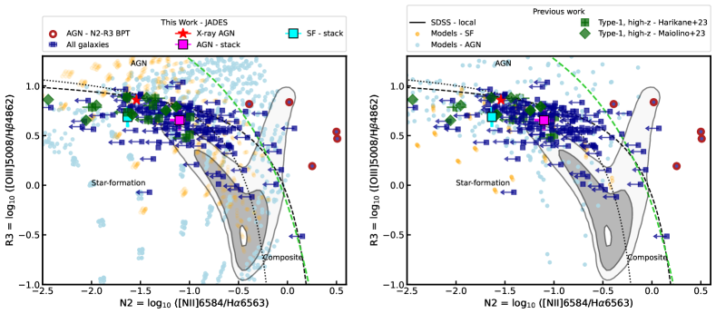
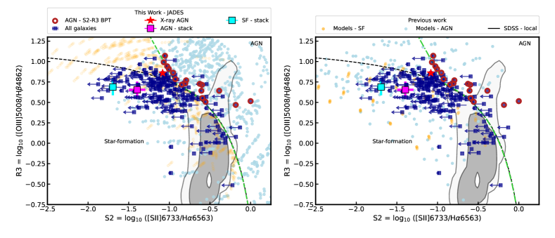
Figure 2: Typical line ratio diagnostic diagrams used to select AGN. N2-R3 BPT ([N ii]/H$\alpha$ vs [O iii]/H$\beta$; top row) and S2-VO87 ([S ii]/H$\alpha$ vs [O iii]/H$\beta$; bottom row). The ionisation models of Feltre et al. (2016); Gutkin et al. (2016) (left) and Nakajima & Maiolino (2022) (right) are reported as yellow (SF) and blue (AGN) points (see §2.4). The objects from this work are plotted as blue squares. The objects selected as AGN based in these diagrams are highlighted by red circles. We also plot our new demarcation lines as green dashed. The black dashed lines show the star forming versus AGN demarcation lines from Kewley et al. (2001) and Kauffmann et al. (2003). For comparison, we plot SDSS galaxies shown as a grey contour plot. The magenta and cyan squares show a stacked spectrum for AGN and star-forming galaxies (see §4.1). We highlight type-1 AGN from Harikane et al. (2023) and Maiolino et al. (2023a) as green squares and diamonds. The red star shows the X-ray selected AGN in our sample.

Table 3: Fitted parameters for equation 1 when fitted for the N2-R3 and S2-R3 diagnostics plot. We define the edge of star-forming galaxies described in §3.1.

Model	a	b	c	d	e
N2-R3	3.08	1.03	2.78	-	-
S2-R3	0.78	0.34	1.36	-0.91	-1.79

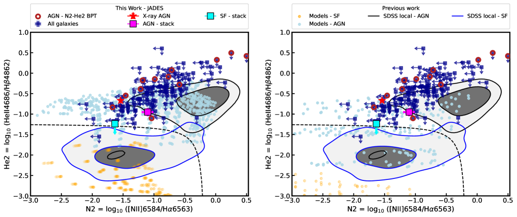
Figure 3: The He2-N2 (He ii /H$\beta$ vs [N ii]/H$\alpha$) diagram for the sample of JADES galaxies for our sample, plotted as blue squares. The left and right plots show ionisation models from Feltre et al. (2016); Gutkin et al. (2016) and Nakajima & Maiolino (2022), respectively, as yellow and light blue points (see §2.4). The magenta and cyan squares show a stacked spectrum for AGN and star-forming galaxies (see §4.1). The black dashed line indicates a demarcation line between star-forming and AGN galaxies by Shirazi & Brinchmann (2012). The blue and black contours show the star-forming galaxies and AGN from SDSS, respectively. We highlight the selected AGN in this diagram with a red circle.

Shirazi & Brinchmann (2012), Tozzi et al. (2023) and Dors et al. (2023) investigated the identification of AGN in SDSS using the He ii $\lambda$4686 emission line. This is a recombination line whose flux is nearly independent of the gas metallicity and ionization parameter, depending instead primarily on the shape of the ionizing spectrum and, more specifically, on the number of ionizing photons with energies beyond 54 eV. We plot the He2-N2 diagram in Figure 3. In this case, we do not redefine the demarcation line as defined by Shirazi & Brinchmann (2012) as the original line is more conservative than the photo-ionisation models used in our work. Overall, we detect He ii $\lambda$4686 in nine galaxies, whose HeII/H$\beta$ ratio indicates the presence of hard ionising radiation indicating AGN. Despite the deep JWST observations, the upper limits on He ii $\lambda$4686/H$\beta$ do not provide any constraints on the presence of an AGN. We note that we selected three additional sources solely based on their N2 ratio $>0.2$ (see Figure 2). Although these sources do not have He ii $\lambda$4686 detections, their large N2 ratio is already identified with the N2-BPT. In summary, based on this diagram we select 12 AGN in total.

We finally note that the only X-ray detected AGN in our sample (red star in Figures 2 and 3) is located in the star-forming region of the N2-BPT and S2-VO87 diagnostic diagrams (hence it would have been missed by this classification, as most type 1 AGN, as discussed in Harikane et al., 2023; Maiolino et al., 2023a; Kocevski et al., 2023), while the upper limit on the HeII$\lambda$4686 would no identify as AGN, further showing complexity of selecting AGN at high redshift.

3.2 Selecting AGN based on UV line diagnostics

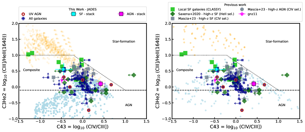
Figure 4: C iii]/He ii $\lambda$1640 vs C iv/C iii](CHe2-C43) diagnostic diagram. We plot our sample as blue squares. The left and right plots show ionisation models from Feltre et al. (2016); Gutkin et al. (2016) and Nakajima & Maiolino (2022), respectively, as yellow and light blue points (see §2.4). The green diamonds show He ii $\lambda$1640 detection from the VANDELS survey (Saxena et al., 2020), and all C iv detections from Mascia et al. (2023) as grey colour with squares and circles representing SF and AGN, respectively. The green squares show local analogues of high-redshift galaxies (from CLASSY survey; Mingozzi et al., 2023). We also show the black dashed and dotted demarcation lines between AGN, star-forming galaxies and composite line ratios from Hirschmann et al. (2022). Overall, we select five AGN on this diagram and we highlight these with a red circle. The magenta and cyan squares show a stacked spectrum for AGN and star-forming galaxies (see §4.1).

In the previous section, we showed that the selection of AGN at high-z using the BPT and S2-VO87 diagrams is extremely challenging for all but metal-rich galaxies. In this section, we will focus on the UV emission lines. The clearest signature of AGN activity is high-ionisation lines such as NV$\lambda$1240, [Ne iv] $\lambda$2424, [Ne v] $\lambda$3426 (Feltre et al., 2016). They require high energy photons (77, 98 and 68 eV, respectively), that can hardly be produced by star-formation processes and are not seen even in galaxies hosting WR stars (Mingozzi et al., 2023); hence, as already mentioned, these are clear signatures of AGN. However, they are often very faint even in powerful AGN (Übler et al., 2023).

Past works on this topic have suggested various UV emission lines ratios based on C iii]$\lambda\lambda$1907,09, C iv$\lambda\lambda$1548,51, [O iii] 1660,66 and He ii $\lambda$1640 (Feltre et al., 2016; Hirschmann et al., 2022; Mingozzi et al., 2022; Mascia et al., 2023). These lines are ideal in identifying AGN at z$>6.8$, where most rest-frame optical emission lines are redshifted out of the wavelength range of JWST/NIRSpec. However, even in luminous AGN the majority of these lines are beyond detectability for a 4-7 hour JWST/NIRSpec exposure at high redshift.

Therefore, in this work, we focus mainly on the brightest emission lines of the UV emission lines that are potentially detectable in our data, or on which we can at least obtain meaningful upper limits. In Figure 4, we show the ratio C iii]$\lambda\lambda$(1906+1908)/He ii $\lambda$1640 (C3He2) against C iv1548,50/C iii]$\lambda\lambda$(1906+1908) (C43). We also plot the models of AGN and star-forming galaxies as blue and orange points, respectively, from Feltre et al. (2016); Gutkin et al. (2016) (left plot) and Nakajima & Maiolino (2022) (right plot). The black and dotted lines show the demarcation lines between star-forming galaxies, AGN, and composite objects derived by Hirschmann et al. (2022). They obtain such a line from the post-processing of the Illustris TNG cosmological simulation using the models of Gutkin et al. (2016) and Feltre et al. (2016). In our sample, there are six targets for which we detect He ii $\lambda$1640. Out of these five objects, one lies in the AGN part of the diagram. Furthermore, four targets are in the composite part of the diagram according to Hirschmann et al. (2022), but they are classified as AGN based on Feltre et al. (2016) and Nakajima & Maiolino (2022).

We also show the objects from Saxena et al. (2020) with He ii $\lambda$1640 detection in the VANDELS survey (McLure et al., 2018) as green diamonds. This sample removed all X-ray-detected objects, removing any signs of obvious AGN. However, most of the type-1 AGN detected with JWST do not show any X-ray emission even in the deepest observations (Maiolino et al. in prep), indicating that many of these VANDELS sources might have a significant AGN contribution. All the VANDELS sources would be classified as AGN by Feltre et al. (2016); Gutkin et al. (2016); Nakajima & Maiolino (2022), whereas 14 of them fall in the AGN or composite region defined by Hirschmann et al. (2022). We also show C iv detections from VANDELs survey (Mascia et al., 2023) as grey squares and circles representing SF and AGN host (identified from X-ray or as type-1 AGN) galaxies, respectively. The AGN and SF galaxies from Mascia et al. (2023) are well separated on our diagram as predicted by the photo-ionisation models used in our work.

We compare our observations with local high-redshift analogues from the CLASSY survey (Berg et al., 2022; James et al., 2022), specifically the data from Mingozzi et al. (2023). The CLASSY sources are classified as star-forming galaxies based on the BPT and He ii $\lambda$4686 optical emission lines. Overall, the five objects in our sample with He ii $\lambda$1640 selected as AGN in our sample have significantly lower C3-He2 ratios than other ”pure” star-forming galaxy samples, confirming our AGN selection.

We note that Mascia et al. (2023) devised a classification of UV-BPT using the VANDELS survey. However, most of the diagnostics diagrams used in that work use both C iv and He ii $\lambda$1640 in the same emission line ratio. Unfortunately, the majority of our sample is undetected in both C iv and He ii $\lambda$1640 which does not allow us to place these objects on their diagnostics diagram. We will further investigate these diagnostics with the full JADES sample in future works.

We note that the above emission line diagnostic requires the detection of three UV emission lines. Despite the excellent sensitivity of JWST/NIRSpec, detecting all three emission lines is still a challenge for exposures $<$10 hours.

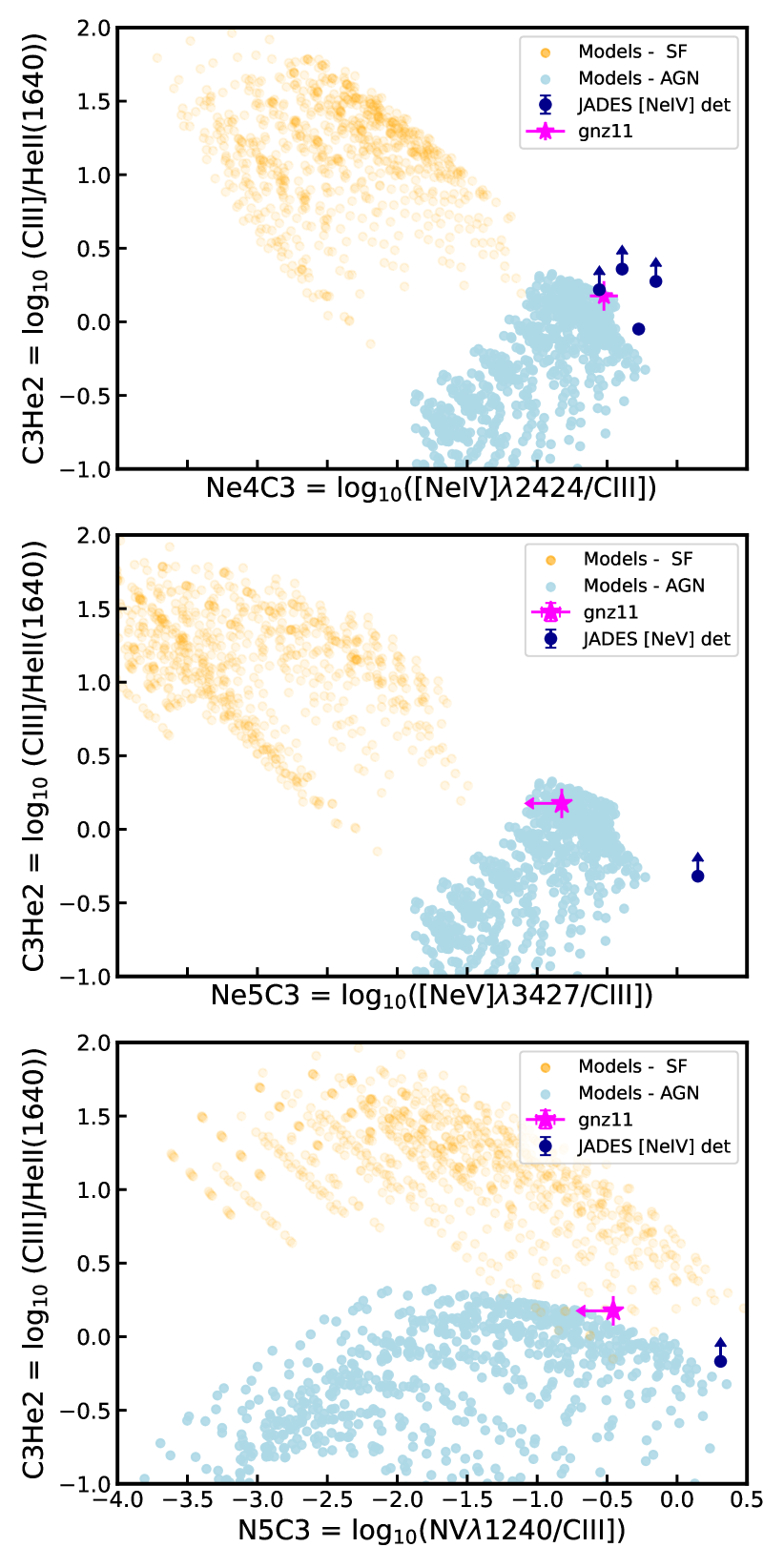
Figure 5: Emission line diagnostics plot for UV high ionisation lines. - Top panel: C3He2 vs [Ne iv] $\lambda$2424/C iii]; Middle Panel: C3He2 vs [Ne v] $\lambda$3427/C iii]diagnostic diagram; Bottom panel: C3He2 vs N V $\lambda$1240/C iii]. We plot our objects detected in high ionisation lines as blue points. The yellow and light blue points show star forming and AGN from photo-ionisation models from Feltre et al. (2016); Gutkin et al. (2016) (see §2.4). We highlight the emission line ratios of GN-z11 (Maiolino et al., 2023b) as the magenta star.

We detect [Ne iv] $\lambda$2424 in five objects. We plot these sources in the top panel of Figure 5, showing C3He2 vs [Ne iv] $\lambda$2424/C iii] as blue points, together with the photo-ionisation models of Gutkin et al. (2016) and Feltre et al. (2016) as yellow and blue points, respectively. All of these four sources have extremely high log₁₀([Ne iv] $\lambda$2424/C iii] ) ratio ($>-0.6$) indicating that these sources are ionised by AGN. The fifth source (ID JADES-NS-GS-1000626) is poorly constrained in both C iii] and He ii $\lambda$1640, and therefore we do not show it on this diagram.

We detect [Ne v] $\lambda$3427 and NV$\lambda$1240 in the objects JADES-NS-GS-10013609 and JADES-NS-GS-00021842, respectively. In both cases, the detections are secured at SNR$\sim$4.5. However, the objects do not have solid detections of either He ii $\lambda$1640 or C iii] . The non-detections of C iii] put a lower limit on the log([Ne v] $\lambda$3420/C iii] ) or log(N V $\lambda$1240/C iii] ) of $>$0. According to Feltre et al. (2016), this lower limit is on the border of what can be reasonably predicted by AGN photo-ionisation models. The N V $\lambda$1240 detection can be potentially explained by star formation, assuming a very high logU=-0.5, which is inconsistent with that measured from [O ii] and [O iii] (logU=-2). As such, we identify JADES-NS-GS-00021842 as an AGN. It is necessary to observe these objects with deep rest-frame UV spectroscopy to help constrain the next geeneration of photo-ionisation models.

4 Discussion

In the previous section, we presented the selection of AGN in the JADES HST Deep survey. Overall, we selected 42 AGN candidates, from at least one of the different selection methods investigated in Section 3, in our parent sample of 209 galaxies (defined in §3) in the redshift range of 1.4–9.4. The final fraction of type-2 AGN in the galaxy population is up to 20%. In this section, we discuss our results and their implications. In §4.1 we perform spectral stacking to find average emission line properties of AGN and star-forming galaxies, in §4.2 we compare the different selection methods used in this work, in §4.4 we investigated the AGN bolometric luminosities, in §4.5 we compare the SFR and stellar masses of AGN to those of star-forming galaxies and finally in §4.6 we discuss the contribution of AGN host galaxies to the UV luminosity function.

4.1 Stacking

In order to get the average emission line properties of our star-forming and AGN samples, we stacked the R1000 grating spectra for each of the emission lines used in our emission line diagnostics. Although the PRISM observations are deeper, the vastly varying spectral resolution as a function of wavelength makes any stacking efforts challenging. Furthermore, some of the emission lines we are interested in (such as [NII], He ii 1640) would be blended with other emission lines. Also, we only stack spectra from the 1210 program, since the 3215 observations lack band-2 observations (see discussion in §4.2). As such, this would bias the stack against redshifts where the key emission lines are redshifted to band-2.

We stack the AGN hosts and star-forming galaxies in two separate stacks: a rest-frame UV emission line stack (C iv, HeII$\lambda$1640 and C iii]) and a rest-frame optical one (HeII$\lambda$4685, H$\beta$, [O iii], H$\alpha$, [N ii] ). For each of these two cases, we stack all sources with available R1000 coverage of these emission lines. Overall, we stack 9 and 20 AGN, and 31 and 55 star-forming galaxies (i.e. the parent sample type-1 and type-2 AGN) in the UV and optical emission line sets, respectively, using only the 1210 program. As shown with type-1 AGN, some objects can be low luminosity AGN that is not selected using any of our diagnostics. As such, the star-forming galaxy sample can be contaminated by unidentified AGN.

The stacking was performed by first shifting all spectra to the rest-frame and rebinning them to a common wavelength grid using Python’s spectres package (Carnall, 2017). We then model and subtract the continuum with a single power law. This is an appropriate model for the continuum, as we are only fitting a narrow wavelength range, and the continuum is poorly detected in the R1000 spectra. The individual spectra are weighted using two separate weighting schemes: a) 1/rms² weights; and b) 1/(rms${}^{2}\times$ F_[OIII]) or 1/(rms${}^{2}\times$ F_CIII]) weights for the UV line stacking) weights. However, given the large range of redshifts and galaxy luminosities, we found that the final stacked spectra are dominated by bright targets when we do not normalise by line fluxes. Hence, we will use the stacked spectra weighted by both the noise and the line fluxes ([O iii] or C iii]), which approximates a median stacked spectrum.

The measured fluxes and their uncertainties for the HeII$\lambda$4685, H$\beta$, [O iii], H$\alpha$, [N ii] and UV emission lines: CIV, HeII$\lambda$1640 and C iii]$\lambda$1907,1909 along with the number of objects in the stack and their median redshift are summarised in the Table 4. The final stacked spectra and the best fits are shown in the Appendix in Figures 12 and 13. We detect all emission lines across all samples at $>3\sigma$, except for He ii $\lambda 4686$ in the star-forming galaxy sample. The detection of [N ii] seems like a contradiction compared to Cameron et al. (2023b), however, this is purely due to the inclusion of galaxies with z¡4, while Cameron et al. (2023b) restricted their sample to $z>5.5$.

We show the line ratios from the stacked spectra in all diagnostic diagrams for the AGN and star-forming samples as magenta and cyan squares in Figures 2, 3 and 4.

The stacked spectra on the N2-BPT (see top panel of Figure 2) show that AGN at high-z are [N ii] weak and have a [O iii]/H$\beta$ ratio very similar to star-forming galaxies, making the selection of AGN at high-z impossible using this method. Furthermore, the AGN host galaxies have the same [S ii]/H$\alpha$ ratios as star-forming galaxies (see bottom panel of Figure 2), further showing the difficulty of using this diagram to select AGN at high-z.

We do not detect the He ii $\lambda$4686 in the star-forming galaxies, and therefore we place a 3$\sigma$ upper limit on the flux. The He ii $\lambda$4686/H$\beta$ vs [N ii]/H$\alpha$ diagram shows a separation of star-forming and AGN galaxies as expected based on the study by Shirazi & Brinchmann (2012) that focused on SDSS galaxies. As such, the He ii $\lambda$4686 line is an ideal tracer of AGN activity; however the He ii $\lambda$4686 is a factor of 7 fainter than He ii $\lambda$1640, making it extremely difficult to detect, even with JWST.

We detect He ii $\lambda$1640 in both star-forming and AGN-dominated galaxies, although the flux of He ii $\lambda$1640 is three times higher in AGN compared to star-forming galaxies. Furthermore, the C iv emission line is a factor of eight brighter in AGN than in the star-forming galaxies. This indicates a much higher and harder ionisation field in AGN host galaxies, boosting the high ionisation lines. However, the stacked spectrum of star-forming galaxies shows He ii $\lambda$1640, with the star-forming stack in the border of AGN and star-forming galaxies on the C iii]/C iv vs C iii]/He ii $\lambda$1640 diagnostic plot (see Figure 4). This can be due to some low luminosity AGN in the star-forming sample that do not have individual He ii $\lambda$1640 detections, or because star-forming galaxies at high-z are creating more hard ionising photons than previously modelled.

Table 4: Results of the stacking analysis for UV and optical emission lines of star-forming and AGN samples.

Sample	AGN	AGN	SF	SF
	Optical	UV	Optical	UV
N	20	9	55	31
zmedian	3.87	5.93	4.77	5.91
Fluxes	($\times$10-20	erg s-1 cm-2)
H$\alpha$	114.5${}^{+1.7}_{-1.6}$	-	66.5${}^{+0.8}_{-0.8}$	-
[N ii]	16.6${}^{+1.0}_{-1.1}$	-	2.5${}^{+0.4}_{-0.4}$	-
[S ii]	4.5${}^{+2.0}_{-1.7}$	-	1.6${}^{+0.5}_{-0.5}$	-
[O iii]	222.2${}^{+1.9}_{-2.0}$	-	113.3${}^{+0.8}_{-0.8}$	-
H$\beta$	48.8${}^{+1.5}_{-1.5}$	-	24.1${}^{+0.6}_{-0.7}$	-
He ii $\lambda$4686	6.6${}^{+1.2}_{-1.1}$	-	$<10.5$	-
C iii]	-	20.7${}^{+3.8}_{-3.7}$	-	16.5${}^{+1.9}_{-1.8}$
C iv	-	59.0${}^{+4.7}_{-4.6}$	-	6.1${}^{+1.7}_{-1.5}$
He ii $\lambda$1640	-	18.6${}^{+3.3}_{-3.3}$	-	4.2${}^{+1.4}_{-1.3}$

4.2 Comparing AGN selection methods

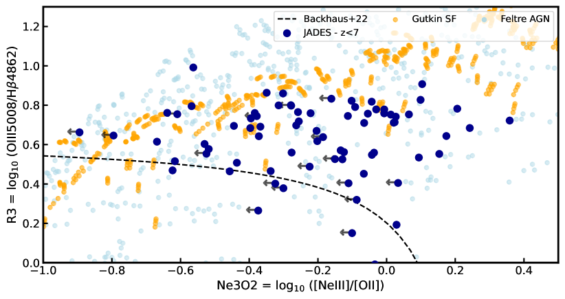
Figure 6: [O iii] /H$\beta$ vs [NeIII]/[OII] diagram (”OHNO”). The black dashed lines show the boundary between AGN and star forming galaxies from Backhaus et al. (2022). The orange and light blue points show star forming and AGN photoionisation models from Feltre et al. (2016) and Gutkin et al. (2016), respectively. There is a significant overlap between AGN and star forming galaxies in this diagram, making it unreliable to select AGN.

Regardless of the emission diagnostic used to identify AGN (emission lines, X-ray observations, mid-infra-red selection), the selection method is reliant on finding emission that cannot be explained by star-formation processes. Objects not selected as AGN, the star-forming galaxies, can still have a significant amount of AGN activity, but it is not dominating the total galaxy emission. Therefore, AGN selection most likely provides an lower limit on the total number of AGN, as we are likely missing low luminosity active black holes, outshone by their host galaxy.

There is little overlap between the individual emission line ratios used to find AGN in this work, with only five objects being selected in more than one diagnostic. This can be explained by the different emission line ratios being more or less sensitive to AGN activity in different observed regimes (e.g. redshift and metallicity of the ISM). As discussed above, the N2-BPT method becomes increasingly unreliable towards high redshift as galaxies become more metal-poor and have higher ionisation parameters. Although the highest redshift AGN selected by this method is at z=5.135 (JADES-NS-GS-00009452; 12+log(O/H)= 7.92), the bulk of the AGN selected by this method are below z=2.3.

Topping et al. (2020); Runco et al. (2021) investigated the effect of stellar population age and metallicity on the BPT and S2-VO87 diagrams. These works have found that a population of young, metal-poor stellar populations can lie above the Kewley et al. (2001) line. These low S2 ratio targets would be excluded from selection with the new definition of the demarcation lines and the AGN selected in the S2-VO87 diagram are above the points seen in both Topping et al. (2020); Runco et al. (2021) (see also Strom et al., 2017). However, many of our selected AGN are very close to the demarcation line, making their selection tentative. As a result, we select any AGN selected within a distance of 0.1 dex from the demarcation as tentative, and we mark this with asterisks in Table 2. We note that our conclusions do not change whether we include or exclude these tentative AGN in our final sample.

In both sets of observations (1210 and 3215) we select more AGN using the S2-VO87 diagram (with [S ii] emission line) than the classical BPT diagram (using [N ii] emission line). The [S ii] doublet is not blended with H$\alpha$ in the PRISM observations at $z<5$, and hence we can use the deeper PRISM observations to constrain [S ii] doublet. On the contrary, the [N ii] doublet is blended with H$\alpha$ in the PRISM observations, and hence we require the shallower R1000 JADES observations to put constraints on it. This is especially taxing for the 3215 observations, which were designed to observe galaxies at z$>6$ and hence do not have any R1000 Band 2 observations. This results in no constraints on the [N ii] doublet for z = 1.8–3.6 in the 3215 program, and hence low detection of AGN on the BPT diagram in this program.

Luckily, as we push our AGN selection to higher redshifts, many useful UV lines ([Ne iv] $\lambda$$\lambda$2424, [Ne v] $\lambda$3427, N V $\lambda$1240, He ii $\lambda$1640) are redshifted into the wavelength range of NIRSpec, and then to a higher sensitivity range of NIRSpec ($\lambda>1.2\mu$m). As a result, the majority of the AGN selected above z=3 are based on [Ne iv] $\lambda$$\lambda$2424, [Ne v] $\lambda$3427, N V $\lambda$1240, He ii $\lambda$1640. Still, these essential emission lines for identifying AGN activity at high redshift remain difficult to detect with JWST. Many of the emission lines such as N V $\lambda$1240, He ii $\lambda$1640 are blended with nearby emission lines in the PRISM observations and require R1000 observations to deblend, which are shallower in JADES survey compared to the PRISM observations. Dedicated ultra-deep R1000 observations are required to detect these lines, even in moderate luminosity AGN.

The HeII$\lambda$4686 emission line remains a robust diagnostic to detect AGN across large redshift and metallicity ranges. However, it is intrinsically fainter by a factor $\sim$10 compared to the HeII$\lambda$1640, resulting in it being a challenge to detect even in deep JWST spectra. However, if detected at high redshift, it is an unambiguous tracer of AGN activity at high redshift.

It is important to point out that these high-ionization lines do not trace AGN activity as such, but a hard ionising radiation, with which AGN activity is the most likely source in galaxy evolution. However, other sources can also produce He ii emission such as Wolf-Rayet stars, X-ray binaries, and some more exotic star-formation processes (e.g. very top-heavy IMF; Thuan & Izotov 2005; Kehrig et al. 2015; Schaerer et al. 2019; Umeda et al. 2022). However, the WR stars produce very broad He ii forming so-called ”blue bump” (see Brinchmann et al. 2008) features not observed in any of our sources. Furthermore, Saxena et al. (2020) indeed reproduced their detections of He ii in the VANDELS survey using implementations of binary stars using BPASS models. However, the AGN and SF galaxies from the same VANDELS survey (Mascia et al., 2023) show the separation of the SF and AGN host galaxies predicted by the Gutkin et al. (2016) and Feltre et al. (2016) models. Nakajima & Maiolino (2022) models, which we use as a comparison of our data, also use BPASS to implement hard ionising photons from binary stars. Meanwhile, high-luminosity AGN at high redshift, such as type-1 AGN at z$\sim$5.5 from Übler et al. (2023) do show features of relatively weak He ii $\lambda$4686 (log₁₀(He ii $\lambda$4686/H$\beta$ )$\sim-1.2$), showing that even objects with relatively weak HeII can be AGN. Finally, Cameron et al. (2023a) identified one of our AGN (ID 9422) to be dominated by nebular continuum. This will be addressed in a separate paper in more detail (Tacchella et al. in prep).

Larson et al. (2023) investigated the use of ”OHNO” diagram ([O iii] /H$\beta$ vs [NeIII]/[OII]) to replace the N2-BPT diagram in selecting AGN. We plot the Cloudy photoionisation models in Figure 6 with JADES galaxies. There is a significant overlap between AGN and star-forming galaxies in this diagram. The one galaxy with [O iii] /H$\beta$¿0.95 lies in the region only populated by AGN Cloudy models is 16745 at $z=5.56$. Overall, in agreement with Larson et al. (2023), we confirm that it is difficult to differentiate between AGN and metal-poor high ionisation star-forming HII regions in the OHNO diagram. For this reason, we need to rely on higher ionisation lines.

Finally, Maiolino et al. (2023a) recently published a sample of type-1 AGN observed with two sources overlapping with our observations. We detected only one as an AGN based on emission line diagnostics (JADES-NS-GS-0008083). Although it was selected by detection of both HeII$\lambda$4686 and NeIV, the other AGN (with log(L${}_{\rm Bol}=44.3$)) is not selected in any of the narrow emission line diagnostics. As already discussed above, it is important to stress that emission line diagnostics miss AGN at high redshift. This can be attributed to 1) the physical properties of high-z AGN being either different from local templates (especially because of low metallicity); 2) these AGN not properly modelled by photoionization models (hence not predicted by the diagnostics); or 3) the emission from these sources is dominated by star-formation in the host galaxy (see Silcock et al. in prep).

4.3 AGN fraction with deeper and shallower data

Across the two observational programs, we selected 28 and 14 AGN from the parent samples of 110 and 99 galaxies, respectively. This corresponds to an AGN fraction of 24$\pm$5 % and 14$\pm$4 %, and a combined AGN fraction from the two programs of 20$\pm$3 %. In Figure 7, we show the AGN fraction as a function of redshift. We plot the AGN fraction from 1210 and 3215 programs as red stars and squares and the combined dataset as blue points. The AGN fraction is consistent with being constant across all redshifts within 1$\sigma$.

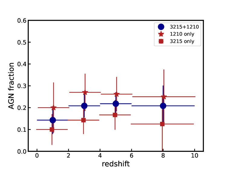
Figure 7: Fraction of AGN as a function of redshift in our survey. The blue points show the fraction resulting from the combined programs (1210+3215) while the red stars and squares show separately the 1210 and 3215, respectively. The red points are offset by 0.05 in the x-axis for better visibility. We see no significant evolution of the AGN fraction as a function of redshift.

The fraction of AGN between the two tiers is consistent within 1.5$\sigma$ of each other. Although this difference is statistically not significant, it is worth discussing the apparent decrease of AGN in the 3215 program, despite this program being a factor of 1.5-3$\times$ deeper than 1210 program. In the 3215 observations, only two AGN host galaxies were selected based on He ii $\lambda$4686, compared to nine in the 1210 program. This is primarily due to the lack of Band 2 R1000 observations in 3215, which results in no constraints of He ii $\lambda$4686 for redshifts 2.8–5.4. As discussed above, this similar issue is also plaguing the BPT selection using the [N ii] emission line, and hence we do not select any AGN using the diagnostics in BPT either.

The Band 1 R1000 observations, which are key to observing rest-frame UV emission lines such as C iii], He ii $\lambda$1640 and C iv doublet, are only a factor of $\sim$1.4 deeper (twice the exposure time) in 3215 than in 1210. Unfortunately, this improvement in sensitivity is not enough to constrain the He ii $\lambda$1640 in regular SF galaxies or less extreme AGN. We would thus require deeper rest-frame UV observations to constrain the AGN and star-forming populations (over 50 hours with JWST/NIRSpec).

4.4 AGN luminosities

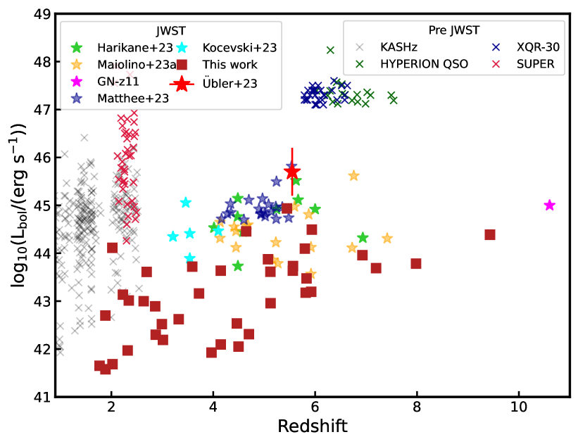
Figure 8: Bolometric luminosity vs redshift for our objects, plotted as red squares. Our bolometric luminosities are estimated from narrow line emission lines and should be treated as upper limits. We compare our sample with previous JWST type-1 AGN (various coloured stars Harikane et al., 2023; Kocevski et al., 2023; Maiolino et al., 2023a, b; Matthee et al., 2023; Übler et al., 2023), AGN from the KASHz and SUPER surveys at Cosmic Noon (grey and red crosses Harrison et al., 2016; Kakkad et al., 2020) and QSOs samples at high at EoR (blue crosses - XQR-30 from Mazzucchelli et al. 2023, green crosses - HYPERION from Zappacosta et al. 2023).

The bolometric luminosity is one of the key properties of AGN and can be easily estimated through the luminosity of the X-ray, BLR or the UV continuum emission from the accretion disc (e.g. Stern & Laor, 2012; Netzer, 2019; Duras et al., 2020; Saccheo et al., 2023). However, as our sources were not selected as Type-1 AGN or X-ray detections, but based on their narrow emission line properties, hence, we do not have the BLR properties of these AGN, nor we have their UV or X-ray flux. As a result, we are forced to use the narrow line emission lines to estimate the bolometric luminosity. We calculate the bolometric luminosities (L_bol) of our sample from the narrow line fluxes of H$\beta$ , [O iii] and C iii] , using the new calibrations by Hirschmann et al. (in prep). The estimated L_bol from all three emission lines agree within 2$\sigma$, however, they are systematically lower by $\sim$0.5 dex compared to the calibration from Netzer (2009).

We present the estimated bolometric luminosities in Figure 8 as a function of redshift, together with other AGN from the literature (both from JWST spectroscopic studies and from previous, non-JWST surveys). However, these luminosities should be considered as upper limits, as they assume that the H$\beta$ and [O iii] or C iii] emission is dominated by the narrow line emission from the AGN, with no contribution from star formation. This is not necessarily true, as AGN are hosted in star-forming galaxies (see §4.5). The estimated bolometric luminosities are reported in Table 2.

As illustrated in Figure 8, pre-JWST studies used large optical and NIR surveys to identify sources dominated by bright rest-frame optical and UV emission, selecting primarily QSOs, or intermediate luminosity AGN at z$<$3. Specifically, in Figure 8, we show luminous quasars at the EoR from Hyperion and XQR-30 samples (Mazzucchelli et al., 2023; Zappacosta et al., 2023) as green and blue crosses and X-ray AGN from the KASHz and SUPER surveys (Harrison et al., 2016; Circosta et al., 2018; Kakkad et al., 2020). Since the launch of JWST, there have been a number of studies searching for AGN using BLR (plotted in Figure 8 as light green, cyan, gold, magenta, dark green and red stars for Harikane et al., 2023; Kocevski et al., 2023; Maiolino et al., 2023a, b; Matthee et al., 2023; Übler et al., 2023, respectively). Our AGN sample has generally similar luminosities to those selected as type-1 AGN with JWST spectroscopic surveys.

With the new capabilities of JWST, we are now probing, at z$>$3, AGN that are 2-3 orders of magnitude less luminous than previous surveys, allowing us to understand the broader demographics of the AGN population in the early Universe for the first time.

4.5 Host Galaxy properties

One of the key questions of studying AGN host galaxies is investigating their star-formation properties. Until the launch of JWST, these studies have mostly focused on $z<3$ moderate luminosity AGN and $z>4$ quasars. These studies have shown that AGN host galaxies have SFR at, or just below, the level of the star-forming galaxies main sequence (SFMS) at Cosmic Noon when mass-matching the active and inactive samples ($z\sim 1-3$; Santini et al., 2012; Rosario et al., 2013; Vito et al., 2014; Mullaney et al., 2015; Stanley et al., 2015; Azadi et al., 2015; Scholtz et al., 2018; Förster Schreiber et al., 2019). With the launch of JWST, we can now select and measure the SFR of moderate luminosity AGN at high redshift. Additionally, unlike previous studies with JWST focusing on type-1 AGN, we do not suffer from the AGN contaminating the continuum emission in our spectra, and hence modeling the stellar SED of the host galaxy is less problematic (although the AGN can still contaminate the Balmer emission lines hence making them less reliable for the SFR estimation).

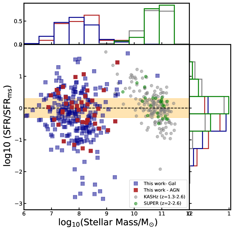
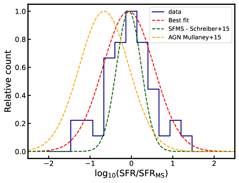
Figure 9: Offset from the star-forming main sequence (SFMS) of our AGN host galaxies. Top panel: Offset from the SFMS against stellar mass for the JADES sample (blue points), our selected AGN (red points). We compare our sample to the previous AGN sample KASHz survey (Harrison et al., 2016, grey points) and SUPER survey (Circosta et al., 2018, green points). We highlight the 1$\sigma$ scatter of SFMS by yellow shaded region. Bottom panel: Distribution of SFR/SFR_MS of the AGN candidates selected in this work. The blue histogram shows the data from this work, and the red dashed line shows the best fit to the distribution of offset from SFMS assuming it is log-normal. The green and orange dashed lines show the distribution for the SFMS (Schreiber et al., 2015) and AGN (Mullaney et al., 2015), respectively.

In §2.3, we described the SED fitting approach adopted to derive the SFR and stellar masses. We use the star-forming main sequence (SFMS) prescription from Looser et al. (2023b), who estimated the SFMS based on 3 separate redshifts bins for sources from JADES with M${}_{*}<10^{9.3}$M_⊙. For AGN at Cosmic Noon, (Harrison et al., 2016; Circosta et al., 2018) we use the SFMS prescription of Schreiber et al. (2015) as it covers the redshift and stellar mass range of our AGN. It is worth mentioning that Schreiber et al. (2015) includes a turnover at high stellar masses.

In Figure 9, we show the offset from the star-forming main-sequence (SFR/SFR_MS) against the stellar mass for AGN and star-forming galaxies in the JADES survey (red and blue points); KASHz AGN survey (grey points) and SUPER AGN survey (green points). The AGN host galaxies in our sample have the same stellar mass distributions as the star-forming galaxies in the JADES HST Deep survey, with a median stellar mass of SF galaxies and AGN are $10^{7.9}$ and $10^{8}$ M_⊙, respectively. The presence of AGN at such low masses indicates that AGN activity is also important in galaxies with M${}_{*}<10^{10}$, as previously suggested by at high redshift (Koudmani et al., 2021, 2022) and low redshift (Burke et al., 2022; Mezcua et al., 2023; Siudek et al., 2023).

The SFRs of our selected AGN are consistent with the star-forming galaxies in the JADES sample. However, measuring the SFR of AGN host galaxies is notoriously difficult (see e.g. Stanley et al., 2015, 2018; Riffel et al., 2021), as AGN can contaminate the emission lines used to estimate SFR. Therefore, many of the SFRs presented in this work should be considered as upper limits. Further SED fitting to disentangle the AGN and star-formation activity will be performed in Silcock et al. (in prep).

To evaluate the difference in the star-formation properties of AGN in our sample, we investigate the distribution of SF_offset. Following Mullaney et al. (2015); Scholtz et al. (2018); Bernhard et al. (2019), we fitted the distribution of SFR/SFR_MS assuming that it is log-normal, with mode and width as free parameters, using an MCMC method. The mode and width of the derived log-normal distribution are $0.07\pm 0.10$ and $0.61\pm 0.07$, respectively. The mode of the distribution is consistent with that of SFMS (mode_SF = -0.07; Schreiber et al. 2015), however, the width is 2$\sigma$ higher than that of SFMS (width of SFMS of 0.3 dex). Some of this difference may be attributed to the methods used to derive SFR (Caplar & Tacchella, 2019). For example, the BEAGLE fitting accounts for physical variations that can lead to variation in the UV to SFR and H$\alpha$ to SFR relationships (see e.g. Curtis-Lake et al. 2021), while the UV and IR SFRs in Schreiber et al. (2015) use simple conversions to SFR.

Mullaney et al. (2015) have measured the distribution of SFR/SFR_MS for X-ray selected AGN at z$\sim$1.6, finding that the mode and the width of the distribution as $-0.36\pm 0.07$ and $0.56\pm 0.09$, respectively. The disagreement between our results and Mullaney et al. (2015) can be attributed to our selection of AGN as well as the fact that SFRs here should be considered upper limits. Furthermore, Mullaney et al. (2015) investigated AGN in massive galaxies (M${}_{*}>10^{10}$M_⊙) at z=1-1.5. The majority of the high-z AGN were selected based on the detection of He ii $\lambda$1640 or He ii $\lambda$4686 which are more likely to be detected in brighter targets.

However, in this work, we do not have a sufficient number of sources to further split our AGN sample by redshift, stellar mass or AGN luminosity. This will be performed in future works with the full JADES sample.

4.6 Contribution of AGN host galaxies to the UV luminosity function

Figure 10: UV luminosity function of galaxies at z=5 from Bouwens et al. (2021) (blue solid line) and inferred contribution of galaxies hosting type-2 AGN, inferred from the JADES survey (red points). Results from other surveys are also reported, as indicated in the legend. The dashed red line shows the galaxy luminosity function scaled downward by a factor of 5. The orange-shaded region shows the range of possible extrapolated luminosity functions for QSOs from Niida et al. (2020).

With this new selection of a large sample of Type-2 AGN, we can now investigate the contribution of AGN host galaxies to the UV luminosity function at high redshifts. We explore the redshift range 4–6, as this is poorly explored in the literature before JWST.

Since the selection function for allocating targets in JADES is complex, it is hard to derive the volume density of AGN host galaxies as a function of the UV luminosity based on the number of AGN that we have identified. More importantly, we do not have high enough statistics to derive a proper luminosity function. Therefore, we make the simplified assumption that the spectroscopic selection function has not preferentially favoured or disfavoured galaxies hosting AGN. We estimate the contribution of AGN host galaxies to the UV luminosity function simply as the fraction of AGN identified in UV luminosity bins.

We choose the parameterised luminosity function from Bouwens et al. (2021) as the reference luminosity function, choosing a median redshift of our type-2 AGN at z=4–6 of z${}_{\rm median}\sim 5.5$ (14 objects in total).

Following the procedure discussed above, we show in Figure 10 (as red points) the UV luminosity function of the type-2 AGN host galaxies z$>4$ from the HST Deep of JADES survey. We split our sample into three separate bins, choosing the bins to allow at least three objects per bin, centred on $M_{UV}=$ -20.15, -18.8, -17.6. The estimated contribution of the type-2 AGN host galaxies to the UV luminosity function is 33 %, 18 % and 20 %, for the $M_{UV}=$ -20.15, -18.8, -17.6 bins, respectively. Given the limited number of points, we do not attempt to fit a functional form, as a small number statistics mean that the parameters are not adequately constrained. Instead, we simply show that the type 2 AGN host galaxies LF can match the Bouwens et al. (2021) galaxy UV luminosity scaled by a factor of 5, as shown by the red dashed line.

We also compare our results with other JWST type-1 AGN surveys: Harikane et al. (2023), Kocevski et al. (2023), Maiolino et al. (2023a), Matthee et al. (2023), as indicated in the legend. The cyan diamonds and squares show the luminosity function inferred by Giallongo et al. (2019) based on X-ray surveys. Given the uncertainties, our estimated type 2 AGN density is slightly higher (by a factor of $\sim$2) than the one estimated for type-1 AGN from the JADES and CEERS surveys (Maiolino et al., 2023a; Harikane et al., 2023). This suggests a type 2 to type 1 AGN ratio of about two at z$\sim$4–6, or possibly higher (given that it is more challenging to identify type 2 AGN). We note that the contribution to the UV luminosity function is significantly higher than the estimate of Kocevski et al. (2023), but which was most likely suffering from a low number of statistics in the early JWST results. The contribution is also higher than found by Matthee et al. (2023), however, as discussed in Maiolino et al. (2023a), that study probe more luminous AGN, hence likely less abundant.

We also note that our estimated density of type-2 AGN is higher than found in the deep X-ray observations by Giallongo et al. (2019). As stated by Maiolino et al. (2023a), this suggests that the optical and UV emission line selection of AGN is picking a population of faint or X-ray deficient population of AGN at high-z. The extrapolation of the QSO luminosity function at z$\sim$5.5 (orange shaded region Niida et al., 2020) is 1–2 orders of magnitude lower than AGN luminosity function from JWST. Together with Figures 8, 9 and 10, this further illustrates that JWST is probing a new parameter space of low luminosity AGN activity at high-z redshift.

We finally point out that our finding that the type 2 AGN host galaxies UV LF can be reproduced by scaling the galaxies LF by a factor of 5, indicates that type 2 AGN host galaxies contribute to $\sim$20% to the reionisation of the Universe ($\sim$30% if including the type 1 AGN). Note that this does not mean that AGN contribute to a similar level to the reionization of the Universe, as the ionizing AGN radiation is obscured along our line of sight, and the IGM sees on average the same fraction of type 2 to type 1 AGN as our line of sight.

4.7 JADES-GS+53.11243-27.77461 - type-2 AGN at z$\sim$9.43

The most distant type 2 AGN in our sample is ID 10058975 (JADES-GS+53.11243-27.77461), which was identified using two separate methods: 1) the detection of [Ne iv] $\lambda$2422 UV emission line; 2) by identifying He ii $\lambda$1640, C iii] and C iv emission line ratios diagnostic. He ii $\lambda$1640 is redshifted to the $\sim$1.71 $\mu$m, which is covered by both Band-1 and Band-2 R1000 grating observations from 1210 observations and Band-1 observations in 3215 observations. We showed the final stacked spectrum from all three observations in Figure 11. The He ii $\lambda$1640 emission line is detected in all three sets of observations, however, we stacked the three spectra for more robust detections (SNR=6.5). The [Ne iv] $\lambda$2424 emission is detected at 4$\sigma$, and we show the spectrum in Figure 14, indicating the presence of strong ionising radiation.

As this object is well detected in all gratings and PRISM observations, we were able to fit the full 1-5 $\mu$m spectrum with BEAGLE. We estimated the stellar mass of the AGN host galaxy to be $1.5\times 10^{8}$ M_⊙ with an SFR of 6.6 M_⊙ yr^-1 (SFR/M${}_{*}=40$ Gyr^-1). The object has a UV magnitude of M${}_{\rm UV}=-20$ and is most likely going through a starburst. However, as discussed above, the high SFR can be explained by the contamination of the emission lines by the AGN, artificially increasing the estimated SFR of the system.

Furthermore, this object has a strong [O iii] $\lambda$4363 emission (5.1$\sigma$ Laseter et al., 2023) at 5.1$\sigma$. This allowed the authors to constrain the electron temperature (T_e) of 18400$\pm$2100K and metallicity 12 + log(O/H)=$7.46\pm 0.11$. Such high temperatures and strong auroral line are anomalous in HII regions, but seen in the NLR of AGN (e.g. Brinchmann, 2023). The full detailed analysis of the [O iii] $\lambda$4363 and [O iii] $\lambda$1661,66 is presented in Curti et al. (in prep.).

The metallicity inferred from the direct method is 4$\sigma$ lower than the value inferred by BEAGLE. Despite the unambiguous detection of an AGN and exquisite data provided by NIRSpec we are still hampered in the characterization of NLR and host for integrated spectra such as this one. More advanced SED fitting of these objects using e.g. BEAGLE-AGN (Vidal-García et al., 2022) is outside the scope of this paper and will be further investigated by Silcock et al. (in prep).

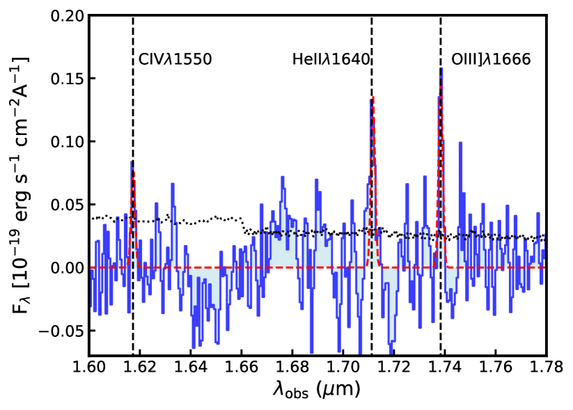
Figure 11: Detection of C iv $\lambda\lambda$ 1548,50, He ii $\lambda$1640 and [O iii] $\lambda$1666 in object ID 10058975 (JADES-GS+53.11243-27.77461) at z=9.43. The spectrum is a combined spectrum of the Band-1 and Band-2 data from program ID 1210 and Band-1 data from program ID 3215 to increase the SNR of the detection. The blue line shows the continuum subtracted observed spectrum, while the red dashed line shows the best fit to the data.

5 Conclusions

In this work we have presented the identification of obscured, i.e. narrow-line (type-2), AGN candidates in the two deepest spectroscopic fields of the JADES survey in GOODS-S, using rest-frame optical and UV emission lines. We have investigated the presence of AGN ionisation, in narrow line emission, by using classical optical N2-R3, S2-VO87, N2-He2 diagnostic diagrams, as well diagrams exploiting UV emission lines: C iii], C iv, He ii $\lambda$1640, [Ne iv] $\lambda$2424, [Ne v] $\lambda$3420 and N V $\lambda$1240.

Based on our analyses we find:

• At z¿3, the N2-BPT and S2-VO87 diagnostic diagrams ([OIII]5007/H$\beta$ vs [NII]6584/H$\alpha$, and vs [SII]6730/H$\alpha$, respectively) are no longer able to clearly distinguish photoionisation due to type-2 AGN and star-forming galaxies, because low metallicity, high-z AGN and star-forming galaxies occupy the same space on these diagrams (see Figure 2). However, we redefine a conservative demarcation line between AGN and star-forming galaxies on the BPT and S2-VO87 diagrams to allow for the shift high redshift star-forming galaxies. We identify five and seventeen AGN host galaxies on the N2-BPT and S2-VO87 diagrams, respectively. We stress that this is a very conservative selection and that many more AGN are certainly present on these diagrams, mixed with star forming galaxies.

• Using the He ii $\lambda$4686/H$\beta$ vs [N ii]/H$\alpha$ diagnostic diagram we selected eleven AGN and an additional six AGN using the C iii]/C iv vs C iii]/HeII$\lambda$1640 diagram (see Figures 3 & 4). Interestingly, the only X-ray detected AGN in our sample, is located in the star-forming region of the BPT diagram, while is confirmed as AGN in the HeII diagnostic diagrams.

• We detected the high ionization transitions [Ne iv] $\lambda$2424, [Ne v] $\lambda$3420 or N V $\lambda$1240 in seven galaxies. The luminosities of these high ionisation lines compared to the C iii]  emission line classify these objects as AGN hosts galaxies.

• In total we selected 28 AGN in the PID-1210 programme and 14 AGN in the PID-3215 programme, resulting in AGN fractions of $24\pm 5$% and $14\pm 4$%, respectively. Combining the two samples, we find 42 unique AGN, and an overall AGN fraction of $20\pm 3$%. We investigated the evolution of AGN fraction as a function of redshift (see Figure 7) and did not find evidence for significant evolution.

• By stacking the AGN and star-forming galaxies’ rest-frame UV and optical spectra we confirmed that both samples have similar emission line ratios in the rest-frame optical N2, S2 and R3 emission line ratios. However, the populations are easily distinguished using the He ii $\lambda$4686 and He ii 1640 emission lines (see cyan and magenta points on Figures 2, 3, 4).

• The estimated bolometric luminosities using narrow-emission lines ([O iii], C iii]and H$\beta$) are in the range of $6\times 10^{41}$–$5\times 10^{45}$ ergs s^-1 (see Figure 8). The selected AGN host galaxies have a median stellar mass of 10^7.9 M_⊙ consistent with the median stellar mass of inactive galaxies of 10^8.0 M_⊙.

• We investigated the distance from the star-forming main sequence, log(SFR/SFR_ms). Our AGN candidates have a mode and width of the distribution of log(SFR/SFR_ms) of $-0.07\pm 0.10$ and $0.61\pm 0.07$, respectively. The mode of distribution is consistent with SF galaxies while the width of the distribution is a factor of two broader than for star-forming galaxies, consistent with previous results at Cosmic Noon.

• We estimated the contribution of the AGN host galaxies to the UV luminosity function on the order of $\sim 20$%, with a slight (increasing) dependence on luminosity (see Figure 10).

Appendix A Stacked spectra

We show the stacked rest-frame UV and optical spectra in Figures 12 and 13 for the AGN and star forming galaxies.

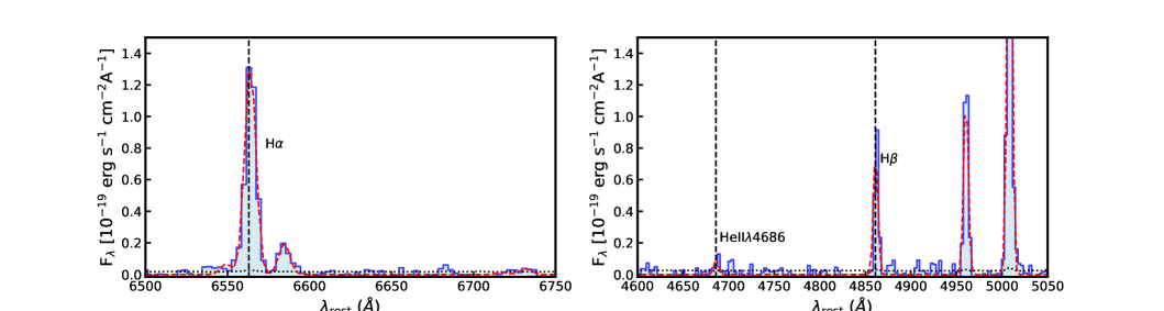
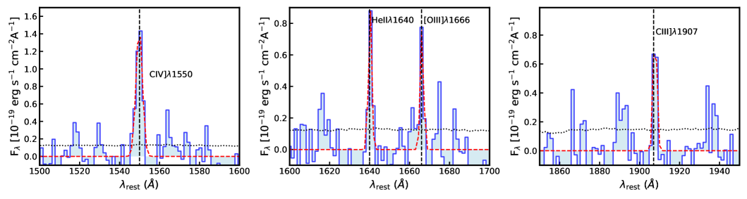
Figure 12: Resulting spectrum from the stacking analysis of AGN host galaxies. The blue line shows the continuum subtracted data, while the red dashed line indicates the best fit to the stacked spectrum. Top row: Stacked spectrum of H$\alpha$, [N ii] and [S ii] (left panel) and He ii $\lambda$4686, H$\beta$ and [O iii] $\lambda$5008 (right panel). Bottom row: Stacked spectrum of C iv (left panel), He ii $\lambda$1640 and [O iii] $\lambda$1666 (middle panel), and C iii] (right panel).

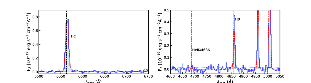
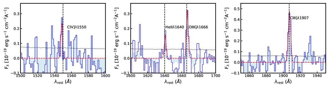
Figure 13: Resulting spectrum from the stacking analysis of star forming galaxies. The blue line shows the continuum subtracted data, while the red dashed line indicates the best fit to the stacked spectrum. Top row: Stacked spectrum of H$\alpha$, [N ii] and [S ii] (left panel) and He ii $\lambda$4686, H$\beta$ and [O iii] $\lambda$5008 (right panel). Bottom row: Stacked spectrum of C iv (left panel), He ii $\lambda$1640 and [O iii] $\lambda$1666 (middle panel), and C iii] (right panel).

Appendix B UV fits

We fit the [Ne iv] $\lambda$2424, [Ne v] $\lambda$3427 and NV$\lambda$1240 emission lines in the § 2.2.1 and we show the spectra for the objects with detected [Ne iv] $\lambda$2424 in Figure 14. Furthermore, we report the fluxes of the detected lines in Table 5.

Table 5: List of AGN and their detected fluxes of high ionisation lines: [Ne iv] $\lambda$2422, [Ne v] $\lambda$3420 and N V $\lambda$1240.

ID	field	Flux [NeIV]$\lambda$2424	Flux [NeV]$\lambda$3427	Flux NV$\lambda$1240
		10-19ergs s-1 cm-2	10-19ergs s-1 cm-2	10-19ergs s-1 cm-2
4902	1210	-	-	-
7099	1210	-	-	-
7762	1210	2.38$\pm 0.67$	-	-
8083	1210	7.50$\pm 1.17$	-	-
8456	1210	-	-	-
8880	1210	-	-	-
9422	1210	-	-	-
9452	1210	-	-	-
10073	1210	-	-	-
16745	1210	-	-	-
17072	1210	-	-	-
17670	1210	-	-	-
21842	1210	-	-	3.48$\pm 0.17$
22251	1210	-	-	-
10000626	1210	5.91$\pm 1.07$	-	-
10008071	1210	-	-	-
10011849	1210	-	-	-
10012477	1210	-	-	-
10012511	1210	-	-	-
10013597	1210	-	-	-
10013609	1210	-	3.37$\pm 0.75$	-
10013905	1210	-	-	-
10015338	1210	-	-	-
10035295	1210	-	-	-
10036017	1210	-	-	-
10040620	1210	-	-	-
10056849	1210	16.75$\pm 1.70$	-	-
10058975	1210	1.88$\pm 0.48$	-	-
95256	3215	-	-	-
99671	3215	-	-	-
104075	3215	-	-	-
108487	3215	-	-	-
111091	3215	-	-	-
111511	3215	-	-	-
114573	3215	-	-	-
132213	3215	-	-	-
143403	3215	-	-	-
201127	3215	-	-	-
202208	3215	-	-	-
208643	3215	-	-	-
209979	3215	-	-	-

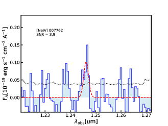
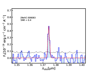
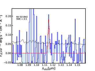
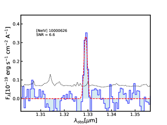
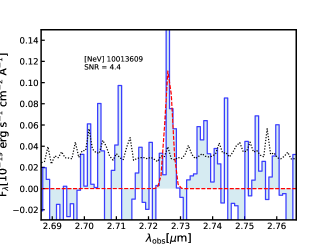
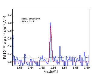
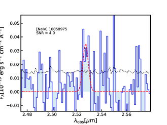
Figure 14: Summary of the detection of [Ne iv] $\lambda$2424, [Ne v] $\lambda$3420 and NV$\lambda$1240. The blue lines show the continuum subtracted observed spectrum, black dotted lines indicate the uncertainties on the flux and the red dashed lines show the best fit to the data.

Appendix C Emission lines used in this work

In Table 6 we summarise the emission lines used in this work, their wavelength and ionisation potential.

Table 6: List of emission lines used in this work, their wavelengths and ionisation potential

Emission line	$\lambda_{\rm rest}$(Å)	Ionisation potential (eV)
[S ii]	6718,32	10.7
[N ii]	6584,48	14.5
H$\alpha$	6563	13.6
[O iii]	5008,4961	35.1
H$\beta$	4861	13.6
He ii	4686	54.4
[O ii]	3727,29	13.6
[Ne iii]	3689	41.0
[Ne v]	3427	97.11
[Ne iv]	2422,24	77.2
C iii]	1907,09	24.4
He ii	1640	54.4
C iv	1548,1550	47.9
[N V]	1239,42	77

References

- Alexander & Hickox (2012) Alexander, D. M. & Hickox, R. C. 2012, New A Rev., 56, 93
- Azadi et al. (2015) Azadi, M., Aird, J., Coil, A. L., et al. 2015, ApJ, 806, 187
- Bañados et al. (2016) Bañados, E., Venemans, B. P., Decarli, R., et al. 2016, ApJS, 227, 11
- Bañados et al. (2018) Bañados, E., Venemans, B. P., Mazzucchelli, C., et al. 2018, Nature, 553, 473
- Backhaus et al. (2022) Backhaus, B. E., Trump, J. R., Cleri, N. J., et al. 2022, ApJ, 926, 161
- Baldwin et al. (1981a) Baldwin, J. A., Phillips, M. M., & Terlevich, R. 1981a, PASP, 93, 5
- Baldwin et al. (1981b) Baldwin, J. A., Phillips, M. M., & Terlevich, R. 1981b, PASP, 93, 5
- Barro et al. (2023) Barro, G., Perez-Gonzalez, P. G., Kocevski, D. D., et al. 2023, arXiv e-prints, arXiv:2305.14418
- Beckmann et al. (2017) Beckmann, R. S., Devriendt, J., Slyz, A., et al. 2017, ArXiv e-prints [arXiv:1701.07838]
- Berg et al. (2022) Berg, D. A., James, B. L., King, T., et al. 2022, ApJS, 261, 31
- Bernhard et al. (2019) Bernhard, E., Grimmett, L. P., Mullaney, J. R., et al. 2019, MNRAS, 483, L52
- Bogdan et al. (2023) Bogdan, A., Goulding, A., Natarajan, P., et al. 2023, arXiv e-prints, arXiv:2305.15458
- Böker et al. (2022) Böker, T., Arribas, S., Lützgendorf, N., et al. 2022, A&A, 661, A82
- Bonaventura et al. (2023) Bonaventura, N., Jakobsen, P., Ferruit, P., Arribas, S., & Giardino, G. 2023, A&A, 672, A40
- Bongiorno et al. (2014) Bongiorno, A., Maiolino, R., Brusa, M., et al. 2014, MNRAS, 443, 2077
- Bouwens et al. (2021) Bouwens, R. J., Oesch, P. A., Stefanon, M., et al. 2021, AJ, 162, 47
- Brinchmann (2023) Brinchmann, J. 2023, MNRAS, 525, 2087
- Brinchmann et al. (2008) Brinchmann, J., Kunth, D., & Durret, F. 2008, A&A, 485, 657
- Bruzual & Charlot (2003) Bruzual, G. & Charlot, S. 2003, MNRAS, 344, 1000
- Bunker et al. (2023a) Bunker, A. J., Cameron, A. J., Curtis-Lake, E., et al. 2023a, arXiv e-prints, arXiv:2306.02467
- Bunker et al. (2023b) Bunker, A. J., Saxena, A., Cameron, A. J., et al. 2023b, A&A, 677, A88
- Burke et al. (2022) Burke, C. J., Liu, X., Shen, Y., et al. 2022, MNRAS, 516, 2736
- Cameron et al. (2023a) Cameron, A. J., Katz, H., Witten, C., et al. 2023a, arXiv e-prints, arXiv:2311.02051
- Cameron et al. (2023b) Cameron, A. J., Saxena, A., Bunker, A. J., et al. 2023b, arXiv e-prints, arXiv:2302.04298
- Caplar & Tacchella (2019) Caplar, N. & Tacchella, S. 2019, MNRAS, 487, 3845
- Cappellari (2017) Cappellari, M. 2017, MNRAS, 466, 798
- Cappellari (2022) Cappellari, M. 2022, arXiv e-prints, arXiv:2208.14974
- Carnall (2017) Carnall, A. C. 2017, arXiv e-prints, arXiv:1705.05165
- Carnall et al. (2023a) Carnall, A. C., McLeod, D. J., McLure, R. J., et al. 2023a, MNRAS, 520, 3974
- Carnall et al. (2023b) Carnall, A. C., McLure, R. J., Dunlop, J. S., et al. 2023b, arXiv e-prints, arXiv:2301.11413
- Chabrier (2003) Chabrier, G. 2003, PASP, 115, 763
- Chevallard & Charlot (2016) Chevallard, J. & Charlot, S. 2016, MNRAS, 462, 1415
- Choi et al. (2018) Choi, E., Somerville, R. S., Ostriker, J. P., Naab, T., & Hirschmann, M. 2018, ApJ, 866, 91
- Choi et al. (2016) Choi, J., Dotter, A., Conroy, C., et al. 2016, ApJ, 823, 102
- Circosta et al. (2018) Circosta, C., Mainieri, V., Padovani, P., et al. 2018, A&A, 620, A82
- Conroy & Gunn (2010) Conroy, C. & Gunn, J. E. 2010, ApJ, 712, 833
- Conroy et al. (2009) Conroy, C., Gunn, J. E., & White, M. 2009, ApJ, 699, 486
- Conroy et al. (2019) Conroy, C., Naidu, R. P., Zaritsky, D., et al. 2019, ApJ, 887, 237
- Crain et al. (2015) Crain, R. A., Schaye, J., Bower, R. G., et al. 2015, MNRAS, 450, 1937
- Curti et al. (2023a) Curti, M., D’Eugenio, F., Carniani, S., et al. 2023a, MNRAS, 518, 425
- Curti et al. (2023b) Curti, M., Maiolino, R., Carniani, S., et al. 2023b, arXiv e-prints, arXiv:2304.08516
- Curtis-Lake et al. (2023) Curtis-Lake, E., Carniani, S., Cameron, A., et al. 2023, Nature Astronomy, 7, 622
- Curtis-Lake et al. (2021) Curtis-Lake, E., Chevallard, J., Charlot, S., & Sandles, L. 2021, MNRAS, 503, 4855
- Di Matteo et al. (2005) Di Matteo, T., Springel, V., & Hernquist, L. 2005, Nature, 433, 604
- Dome et al. (2023) Dome, T., Tacchella, S., Fialkov, A., et al. 2023, arXiv e-prints, arXiv:2305.07066
- Dors et al. (2023) Dors, O. L., Cardaci, M. V., Hagele, G. F., et al. 2023, arXiv e-prints, arXiv:2311.14026
- Dubois et al. (2013a) Dubois, Y., Gavazzi, R., Peirani, S., & Silk, J. 2013a, MNRAS, 433, 3297
- Dubois et al. (2013b) Dubois, Y., Pichon, C., Devriendt, J., et al. 2013b, MNRAS, 428, 2885
- Duras et al. (2020) Duras, F., Bongiorno, A., Ricci, F., et al. 2020, A&A, 636, A73
- Eisenstein et al. (2023a) Eisenstein, D. J., Johnson, B. D., Robertson, B., et al. 2023a, arXiv e-prints, arXiv:2310.12340
- Eisenstein et al. (2023b) Eisenstein, D. J., Willott, C., Alberts, S., et al. 2023b, arXiv e-prints, arXiv:2306.02465
- Eldridge et al. (2017) Eldridge, J. J., Stanway, E. R., Xiao, L., et al. 2017, PASA, 34, e058
- Endsley et al. (2023) Endsley, R., Stark, D. P., Whitler, L., et al. 2023, arXiv e-prints, arXiv:2306.05295
- Fan et al. (2022) Fan, X., Banados, E., & Simcoe, R. A. 2022, arXiv e-prints, arXiv:2212.06907
- Feltre et al. (2016) Feltre, A., Charlot, S., & Gutkin, J. 2016, MNRAS, 456, 3354
- Ferland et al. (2013) Ferland, G. J., Porter, R. L., van Hoof, P. A. M., et al. 2013, Rev. Mexicana Astron. Astrofis., 49, 137
- Ferruit et al. (2022) Ferruit, P., Jakobsen, P., Giardino, G., et al. 2022, A&A, 661, A81
- Förster Schreiber et al. (2019) Förster Schreiber, N. M., Übler, H., Davies, R. L., et al. 2019, ApJ, 875, 21
- Furtak et al. (2023) Furtak, L. J., Labbé, I., Zitrin, A., et al. 2023, arXiv e-prints, arXiv:2308.05735
- Furtak et al. (2022) Furtak, L. J., Zitrin, A., Plat, A., et al. 2022, arXiv e-prints, arXiv:2212.10531
- Gardner et al. (2023) Gardner, J. P., Mather, J. C., Abbott, R., et al. 2023, PASP, 135, 068001
- Gelli et al. (2023) Gelli, V., Salvadori, S., Ferrara, A., & Pallottini, A. 2023, arXiv e-prints, arXiv:2310.03065
- Giallongo et al. (2019) Giallongo, E., Grazian, A., Fiore, F., et al. 2019, ApJ, 884, 19
- Goodman & Weare (2010) Goodman, J. & Weare, J. 2010, Communications in Applied Mathematics and Computational Science, 5, 65
- Greene et al. (2023) Greene, J. E., Labbe, I., Goulding, A. D., et al. 2023, arXiv e-prints, arXiv:2309.05714
- Groves et al. (2006) Groves, B. A., Heckman, T. M., & Kauffmann, G. 2006, MNRAS, 371, 1559
- Gutkin et al. (2016) Gutkin, J., Charlot, S., & Bruzual, G. 2016, MNRAS, 462, 1757
- Harikane et al. (2023) Harikane, Y., Zhang, Y., Nakajima, K., et al. 2023, arXiv e-prints, arXiv:2303.11946
- Harrison (2017) Harrison, C. M. 2017, Nature Astronomy, 1, 0165
- Harrison et al. (2016) Harrison, C. M., Alexander, D. M., Mullaney, J. R., et al. 2016, MNRAS, 456, 1195
- Hirschmann et al. (2022) Hirschmann, M., Charlot, S., Feltre, A., et al. 2022, arXiv e-prints, arXiv:2212.02522
- Hirschmann et al. (2019) Hirschmann, M., Charlot, S., Feltre, A., et al. 2019, MNRAS, 487, 333
- Hirschmann et al. (2014) Hirschmann, M., Dolag, K., Saro, A., et al. 2014, MNRAS, 442, 2304
- Inayoshi et al. (2020) Inayoshi, K., Visbal, E., & Haiman, Z. 2020, ARA&A, 58, 27
- Jakobsen et al. (2022) Jakobsen, P., Ferruit, P., Alves de Oliveira, C., et al. 2022, A&A, 661, A80
- James et al. (2022) James, B. L., Berg, D. A., King, T., et al. 2022, ApJS, 262, 37
- Juodžbalis et al. (2023) Juodžbalis, I., Conselice, C. J., Singh, M., et al. 2023, arXiv e-prints, arXiv:2307.07535
- Kakkad et al. (2020) Kakkad, D., Mainieri, V., Vietri, G., et al. 2020, arXiv e-prints, arXiv:2008.01728
- Kauffmann et al. (2003) Kauffmann, G., Heckman, T. M., Tremonti, C., et al. 2003, MNRAS, 346, 1055
- Kehrig et al. (2015) Kehrig, C., Vílchez, J. M., Pérez-Montero, E., et al. 2015, ApJ, 801, L28
- Kewley et al. (2001) Kewley, L. J., Dopita, M. A., Sutherland, R. S., Heisler, C. A., & Trevena, J. 2001, ApJ, 556, 121
- Kewley et al. (2013) Kewley, L. J., Maier, C., Yabe, K., et al. 2013, ApJ, 774, L10
- Kewley et al. (2019) Kewley, L. J., Nicholls, D. C., & Sutherland, R. S. 2019, ARA&A, 57, 511
- Kocevski et al. (2023) Kocevski, D. D., Onoue, M., Inayoshi, K., et al. 2023, arXiv e-prints, arXiv:2302.00012
- Konstantopoulou et al. (2023) Konstantopoulou, C., De Cia, A., Ledoux, C., et al. 2023, arXiv e-prints, arXiv:2310.07709
- Kormendy & Ho (2013) Kormendy, J. & Ho, L. C. 2013, ARA&A, 51, 511
- Koudmani et al. (2021) Koudmani, S., Henden, N. A., & Sijacki, D. 2021, MNRAS, 503, 3568
- Koudmani et al. (2022) Koudmani, S., Sijacki, D., & Smith, M. C. 2022, MNRAS, 516, 2112
- Larson et al. (2023) Larson, R. L., Finkelstein, S. L., Kocevski, D. D., et al. 2023, arXiv e-prints, arXiv:2303.08918
- Laseter et al. (2023) Laseter, I. H., Maseda, M. V., Curti, M., et al. 2023, arXiv e-prints, arXiv:2306.03120
- Looser et al. (2023a) Looser, T. J., D’Eugenio, F., Maiolino, R., et al. 2023a, arXiv e-prints, arXiv:2306.02470
- Looser et al. (2023b) Looser, T. J., D’Eugenio, F., Maiolino, R., et al. 2023b, arXiv e-prints, arXiv:2306.02470
- Looser et al. (2023c) Looser, T. J., D’Eugenio, F., Maiolino, R., et al. 2023c, arXiv e-prints, arXiv:2302.14155
- Lynden-Bell (1969) Lynden-Bell, D. 1969, Nature, 223, 690
- Lyu et al. (2022) Lyu, J., Alberts, S., Rieke, G. H., & Rujopakarn, W. 2022, ApJ, 941, 191
- Lyu et al. (2023) Lyu, J., Alberts, S., Rieke, G. H., et al. 2023, arXiv e-prints, arXiv:2310.12330
- Magorrian et al. (1998) Magorrian, J., Tremaine, S., Richstone, D., et al. 1998, AJ, 115, 2285
- Maiolino et al. (2023a) Maiolino, R., Scholtz, J., Curtis-Lake, E., et al. 2023a, arXiv e-prints, arXiv:2308.01230
- Maiolino et al. (2023b) Maiolino, R., Scholtz, J., Witstok, J., et al. 2023b, arXiv e-prints, arXiv:2305.12492
- Mascia et al. (2023) Mascia, S., Pentericci, L., Saxena, A., et al. 2023, A&A, 674, A221
- Matthee et al. (2023) Matthee, J., Naidu, R. P., Brammer, G., et al. 2023, arXiv e-prints, arXiv:2306.05448
- Mazzucchelli et al. (2023) Mazzucchelli, C., Bischetti, M., D’Odorico, V., et al. 2023, arXiv e-prints, arXiv:2306.16474
- McLure et al. (2018) McLure, R. J., Pentericci, L., Cimatti, A., et al. 2018, MNRAS, 479, 25
- Merloni et al. (2010) Merloni, A., Bongiorno, A., Bolzonella, M., et al. 2010, ApJ, 708, 137
- Merloni et al. (2004) Merloni, A., Rudnick, G., & Di Matteo, T. 2004, MNRAS, 354, L37
- Mezcua et al. (2018) Mezcua, M., Civano, F., Marchesi, S., et al. 2018, MNRAS, 478, 2576
- Mezcua et al. (2023) Mezcua, M., Siudek, M., Suh, H., et al. 2023, ApJ, 943, L5
- Mignoli et al. (2019) Mignoli, M., Feltre, A., Bongiorno, A., et al. 2019, A&A, 626, A9
- Mingozzi et al. (2022) Mingozzi, M., James, B. L., Arellano-Córdova, K. Z., et al. 2022, ApJ, 939, 110
- Mingozzi et al. (2023) Mingozzi, M., James, B. L., Berg, D., et al. 2023, arXiv e-prints, arXiv:2306.15062
- Mullaney et al. (2015) Mullaney, J. R., Alexander, D. M., Aird, J., et al. 2015, MNRAS, 453, L83
- Nakajima & Maiolino (2022) Nakajima, K. & Maiolino, R. 2022, MNRAS, 513, 5134
- Netzer (2009) Netzer, H. 2009, MNRAS, 399, 1907
- Netzer (2019) Netzer, H. 2019, MNRAS, 488, 5185
- Niida et al. (2020) Niida, M., Nagao, T., Ikeda, H., et al. 2020, ApJ, 904, 89
- Onoue et al. (2023) Onoue, M., Inayoshi, K., Ding, X., et al. 2023, ApJ, 942, L17
- Perna et al. (2023) Perna, M., Arribas, S., Marshall, M., et al. 2023, A&A, 679, A89
- Planck Collaboration et al. (2020) Planck Collaboration, Aghanim, N., Akrami, Y., et al. 2020, A&A, 641, A6
- Rees et al. (1982) Rees, M. J., Begelman, M. C., Blandford, R. D., & Phinney, E. S. 1982, Nature, 295, 17
- Riffel et al. (2021) Riffel, R., Mallmann, N. D., Ilha, G. S., et al. 2021, MNRAS, 501, 4064
- Rigby et al. (2023) Rigby, J., Perrin, M., McElwain, M., et al. 2023, PASP, 135, 048001
- Robertson et al. (2023) Robertson, B. E., Tacchella, S., Johnson, B. D., et al. 2023, Nature Astronomy, 7, 611
- Rosario et al. (2013) Rosario, D. J., Santini, P., Lutz, D., et al. 2013, ApJ, 771, 63
- Runco et al. (2021) Runco, J. N., Shapley, A. E., Sanders, R. L., et al. 2021, MNRAS, 502, 2600
- Saccheo et al. (2023) Saccheo, I., Bongiorno, A., Piconcelli, E., et al. 2023, A&A, 671, A34
- Santini et al. (2012) Santini, P., Rosario, D. J., Shao, L., et al. 2012, A&A, 540, A109
- Saxena et al. (2020) Saxena, A., Pentericci, L., Mirabelli, M., et al. 2020, A&A, 636, A47
- Schaerer et al. (2019) Schaerer, D., Fragos, T., & Izotov, Y. I. 2019, A&A, 622, L10
- Schaerer et al. (2022) Schaerer, D., Marques-Chaves, R., Barrufet, L., et al. 2022, A&A, 665, L4
- Scholtz et al. (2018) Scholtz, J., Alexander, D. M., Harrison, C. M., et al. 2018, MNRAS, 475, 1288
- Scholtz et al. (2023) Scholtz, J., Witten, C., Laporte, N., et al. 2023, arXiv e-prints, arXiv:2306.09142
- Schreiber et al. (2015) Schreiber, C., Pannella, M., Elbaz, D., et al. 2015, A&A, 575, A74
- Segers et al. (2016) Segers, M. C., Schaye, J., Bower, R. G., et al. 2016, MNRAS, 461, L102
- Shen et al. (2019) Shen, Y., Wu, J., Jiang, L., et al. 2019, ApJ, 873, 35