Steering Deep Feature Learning
with Backward Aligned Feature Updates

Abstract

Deep learning succeeds by doing hierarchical feature learning, yet tuning Hyper-Parameters (HP) such as initialization scales, learning rates etc., only give indirect control over this behavior. In this paper, we propose the alignment between the feature updates and the backward pass as a key notion to predict, measure and control feature learning. On the one hand, we show that when alignment holds, the magnitude of feature updates after one SGD step is related to the magnitude of the forward and backward passes by a simple and general formula. This leads to techniques to automatically adjust HPs (initialization scales and learning rates) to attain a desired feature learning behavior. On the other hand, we show that, at random initialization, this alignment is determined by the spectrum of a certain kernel, and that well-conditioned layer-to-layer Jacobians (aka dynamical isometry) implies alignment. Finally, we investigate ReLU MLPs and ResNets in the large width-then-depth limit. Combining hints from random matrix theory and numerical experiments, we show that (i) in MLP with iid initializations, alignment degenerates with depth, making it impossible to start training, and that (ii) in ResNets, the branch scale $1/\sqrt{\text{depth}}$ is the only one maintaining non-trivial alignment at infinite depth.

1 Introduction

The ability of deep Neural Networks (NNs) to learn a hierarchical representation of their input is behind their strong performance in many data-intensive machine learning tasks [LeCun et al., 2015]. Yet, the process via which gradient-based training leads to feature learning remains mysterious and even defies our intuition as some architectures can even reach zero loss without feature learning at all [Jacot et al., 2018]. This limited understanding makes it difficult to design or modify NNs architectures, and begs the development of tools to predict, measure and control feature learning.

To this end, we propose the alignment between the feature updates and the backward pass as a key notion. This notion is a natural candidate for investigation, since for a Stochastic Gradient Descent (SGD) step that leads to hierarchical feature learning, the feature updates and the backward pass should (i) not be orthogonal – as the learnt feature would then not be driven by the loss – (ii) nor should they be aligned – as then feature learning would not be actually hierarchical. Alignment is thus a natural indicator to classify architectures and Hyper-Parameters (HPs), but the usefulness of this notion goes much further. Indeed, we will see that the projections of the feature updates in one SGD step on the backward pass – which we call the backward-aligned feature updates (BAFUs) – can be expressed purely in terms of the magnitude of the forward and backward passes. Thus, when alignment holds, feature learning can be measured and controlled at any time during training, with negligible computational cost. In summary, this notion of alignment allows to divide the difficult problem of quantifying feature learning in two separate problems: asserting alignment on the one hand, and quantifying BAFUs on the other.

Contributions

Our contributions can be summarized as follows:

• We introduce the notion of Backward Aligned Feature Update (BAFU) and a simple formula relating it to two observables that are easy to compute (in theory and in practice): weight matrix contributions and feature sensitivities. See Thm. 2.1 for Multi-Layer Perceptrons (MLPs) with batch-size $1$, and Thm. A.2 for any (non-recurrent) architecture.

• We also introduce the related notion of Backward Feature Angle (BFA), and show that at initialization, BFA can be quantified in terms of the spectrum of a kernel, which we call the Backward to Feature Kernel (BFK) (Thm. 2.4). We also show that well-conditioned layer-to-layer Jacobians, a property known as dynamical (approximate) isometry, guarantees alignment (Prop. 2.6).

• We show that natural desiderata for a good SGD step – stable feature learning and alignment – can be guaranteed by the so-called FSCA-criteria pertaining to the Forward pass, Sensitivities, Contributions and Alignment observables (Thm. 3.1). Apart from alignment, the remaining FSC criteria can be enforced at any time during training, via a method which we name FSC-control. This method involves forward and backward layer normalization and adaptive learning rates.

• Finally, we study the large width-then-depth limit of ReLU MLPs and ResNets. Combining numerical experiments with hints from random matrix theory, we show that (i) in MLPs at random iid initializations, alignment degenerates with depth, making it impossible to start training, and that (ii) in ResNets, the branch scale $1/\sqrt{\text{depth}}$ is the only one maintaining non-trivial alignment at infinite depth.

1.1 Related work

In the past ten years, the theory of NNs has benefited from important insights from asymptotic analyses in the large width and/or depth limits. Our work is in the continuity of those.

Analyses of wide and deep NNs at random initialization led to identifying critical initialization scalings that enable signal propagation [Poole et al., 2016, Hanin and Rolnick, 2018, Hanin, 2018]. They also identified dynamical isometry [Pennington et al., 2018], namely the concentration of the singular spectrum of the layer-to-layer Jacobians around $1$, as an important indicator of training performance. Our analysis gives a concrete justification of the link between dynamical isometry and successful training, as we show that it is related to the alignment between the backward pass and feature updates. These questions have also been studied in ResNets, see e.g. [Hayou et al., 2021, Marion et al., 2022, Li et al., 2021] for signal propagation and [Tarnowski et al., 2019, Ling and Qiu, 2019] for dynamical isometry.

In 2018, two viewpoints for the dynamics of wide NNs where simultaneously introduced: a feature learning limit for two layer MLPs [Mei et al., 2018, Chizat and Bach, 2018, Rotskoff and Vanden-Eijnden, 2018] and a limit without feature learning for general NNs [Jacot et al., 2018, Du et al., 2018, Allen-Zhu et al., 2019]. These works shed light on the crucial role of HP scalings – learning rates and initialization – in the behavior of large NNs [Chizat et al., 2019].

In order to classify HPs scalings, [Yang and Hu, 2021] formulated the maximal update $\mu$-criterion (we enrich this with the alignment criterion in Section 3). This criterion led to a full classification of HP scalings in the infinite hidden width limit (at fixed depth), and singled-out the so-called $\mu$-parameterization ($\mu$P) as ideal for this criterion. We note that, provided alignment holds, our analysis allows in particular to recover $\mu$P in an elementary way. See also the recent preprint [Yang et al., 2023a] for another simple derivation of $\mu$P using matrix spectral norms (but that does not a priori apply to large depth settings). Several works have since shown the practical value of these analyses in predicting the behavior of NNs [Vyas et al., 2023] and improving HP tuning [Yang et al., 2021].

When restricted to the output layer of a NN, our notion of alignment coincides with that studied in Baratin et al. [2021], Atanasov et al. [2021], Lou et al. [2022], Wang et al. [2022] and the BFK we consider coincides with the NTK [Jacot et al., 2018]. Our starting point is an extension of these concepts to study and quantify feature learning at any layer (not just at the output layer). These works study the “large batch-size” setting, which is also a natural next direction for our analysis.

Finally, several recent works have studied feature learning in infinite width and depth NNs, starting with [Jelassi et al., 2023] for MLPs, and [Bordelon et al., 2023, Yang et al., 2023b] for ResNets. The two latter identified the $1/\sqrt{\text{depth}}$ branch scaling as providing desirable properties, in particular that of HP transfer [Yang et al., 2021]. These works take the infinite width limit as a first step in their analysis, before studying the resulting objects, resulting in a technical analysis. In our approach, we first take the step-size to $0$ (as in [Jelassi et al., 2023]) and study in detail the structure of the back-propagation equations, before taking the large width-then-depth limit in the last step.

1.2 Notations

For integers $a,b\in\mathbb{Z}$, we denote $[a:b]=\{a,\dots,b\}$. For any vector $x\in\mathbb{R}^{m}$ we denote by $\|x\|_{\mathrm{rms}}\coloneqq m^{-\nicefrac{{1}}{{2}}}\|x\|_{2}$ its root mean-square (RMS) norm. We use this as a proxy for the typical entry size of a vector, which is justified as long as that vector is dense. We also use $\|\cdot\|_{2}$ (resp. $\|x\|_{\mathrm{rms}}$) to denote $\ell_{2}$/Frobenius (resp. RMS) norms for matrices and tensors. Throughout, we use $\delta X$ (resp. $\delta_{\ell}X$) to denote the variation of a quantity $X$ (resp. due solely to the update $\delta W_{\ell}$ of a single weight matrix) after $1$ SGD step. Finally, for a symmetric matrix $K\in\mathbb{R}^{m\times m}$, we denote its $p$-th spectral moment by

$$M_{p}(K)=\frac{1}{m}\sum_{i=1}^{m}\lambda_{i}^{p}$$ (1)

where $\lambda_{1},\dots,\lambda_{m}\geq 0$ are the eigenvalues of $K$.

2 Backward Aligned Feature Updates (BAFU) in MLPs

Let us present our approach in the simplest setting: we study one SGD step in a multilayer perceptron (MLP) with batch size $1$ without bias/intercepts. These derivations are generalized to any (non-recurrent) architecture and batch-size in Appendix A.

2.1 Backpropagation equations

Given a loss function, the computation of the loss of a $L$-layer MLP on an input $x=f_{0}\in\mathbb{R}^{m_{0}}$ is given by $\bar{f}_{1}=W_{1}x$ and for $\ell\in[1:L-1]$,

$$f_{\ell}=\phi(\bar{f}_{\ell}), \bar{f}_{\ell+1}=W_{\ell+1}f_{\ell}, \mathcal{L}=f_{L}=\mathrm{loss}(\bar{f}_{L})\in\mathbb{R}$$

where the map $\phi:\mathbb{R}\to\mathbb{R}$ acts entrywise on vectors. We assume that $\phi$ admits a selection derivative $\phi^{\prime}$. Here $m_{0}$ is the input width, $(m_{\ell})_{\ell=1}^{L-1}$ are the hidden widths, $m_{L}$ is the output width, and $\forall\ell\in[1:L],\;W_{\ell}\in\mathbb{R}^{m_{\ell}\times m_{\ell-1}}$. The vectors $(f_{v})_{v=1}^{L-1}$ are called the activations and $(\bar{f}_{v})_{v=1}^{L-1}$ are called the preactivations vectors. We represent the computational graph with our notations in Fig. 1.

The backward pass is the computation of all gradients $b_{\ell}\coloneqq\big{(}\frac{\partial\mathcal{L}}{\partial f_{\ell}}\big{)}^{\top}$ and $\bar{b}_{\ell}\coloneqq\big{(}\frac{\partial\mathcal{L}}{\partial\bar{f}_{\ell}}\big{)}^{\top}$. By the chain rule, they are given by $b_{L}=1$ and, for $\ell\in[L-1:1]$,

$$\bar{b}_{L}=\nabla\mathrm{loss}(\bar{f}_{L}), b_{\ell}=W_{\ell+1}^{\top}\bar{b}_{\ell+1}, \bar{b}_{\ell}=\phi^{\prime}(\bar{f}_{\ell})\odot b_{\ell}.$$

where $\odot$ represents entrywise multiplication. A SGD step with layerwise Learning-Rate (LR) $\eta_{\ell}>0$ for $\ell\in[L]$ consists in adding to each weight matrix $W_{\ell}$ the update

$$\delta W_{\ell}=-\eta_{\ell}\nabla_{\ell}=-\eta_{\ell}\bar{b}_{\ell}f_{\ell-1}^{\top}.$$

where $\nabla_{\ell}$ is a shortcut for $\nabla_{W_{\ell}}\mathcal{L}$.

[mode=buildnew, width=1.0]tikz/MLP_backward

Figure 1: Computational graph of the forward and backward passes for a 3-layer MLP.

2.2 The Backward-Aligned Feature Update (BAFU) formula

Feature update

The partial feature update due to the weight update $\delta W_{\ell}$ on a certain feature vector $f_{v}$ for $\ell\leq v$ is given, at first order in $\eta_{\ell}$, by

$$\delta_{\ell}f_{v}\coloneqq-\eta_{\ell}J_{\bar{\ell}\to v}\bar{b}_{\ell}f_{\ell-1}^{\top}f_{\ell-1}$$ (2)

where $J_{\bar{\ell}\to v}=\frac{\partial f_{v}}{\partial\bar{f}_{\ell}}\in\mathbb{R}^{m_{v}\times m_{\ell}}$ is the Jacobian matrix (we also use the transparent notations $\delta\bar{f}_{v}$, $J_{\ell\to\bar{v}}$, $J_{\ell\to v}$, etc). In the non-differentiable case, the interpretation as a first order approximation is in general lost, and we directly take Eq. (2) as the definition. The (total) feature update is then given by

$$\delta f_{v}=\sum_{\ell\leq v}\delta_{\ell}f_{v}.$$

Computing this quantity in practice would require to compute the forward pass on the same batch twice in a row, which is a significant overhead. As we show next, this is not the case for the component of $\delta f_{v}$ aligned with $b_{v}$.

Backward-Aligned Feature Update (BAFU).

By definition, the partial BAFU $\delta^{\mathrm{a}}_{\ell}f_{v}$ is the projection of $\delta_{\ell}f_{v}$ on $\operatorname{span}\{b_{v}\}$, and is given by

$$\delta^{\mathrm{a}}_{\ell}f_{v}=\frac{b_{v}^{\top}\delta_{\ell}f_{v}}{\|b_{v}\|_{2}^{2}}b_{v}.$$ (3)

The (total) BAFU $\delta^{\mathrm{a}}f_{v}$ is defined analogously. At the heart of our approach lies the following computation, which can be interpreted as completing the second forward pass:

$$\|\delta_{\ell}^{\mathrm{a}}f_{v}\|_{2}=-\frac{b_{v}^{\top}\delta_{\ell}f_{v}}{\|b_{v}\|_{2}}=\frac{\eta_{\ell}b_{v}^{\top}J_{\bar{\ell}\to v}\bar{b}_{\ell}f_{\ell-1}^{\top}f_{\ell-1}}{\|b_{v}\|_{2}}=\frac{\eta_{\ell}\|\nabla_{\ell}\|^{2}_{2}}{\|b_{v}\|_{2}}$$ (4)

where we used $\bar{b}_{\ell}^{\top}=b_{v}^{\top}J_{\bar{\ell}\to v}$ which is the chain-rule $\frac{\partial\mathcal{L}}{\partial\bar{f}_{\ell}}=\frac{\partial\mathcal{L}}{\partial f_{v}}\frac{\partial f_{v}}{\partial\bar{f}_{\ell}}$, and the fact that the squared gradient norm is $\|\nabla_{\ell}\|^{2}_{2}=\operatorname{tr}\big{(}(\bar{b}_{\ell}f^{\top}_{\ell-1})^{\top}(\bar{b}_{\ell}f^{\top}_{\ell-1})\big{)}=\|\bar{b}_{\ell}\|_{2}^{2}\cdot\|f_{\ell-1}\|_{2}^{2}$. The negative sign that appears is justified by the fact that the last quantity is nonnegative.

BAFU formula

Our next step is to switch from $\ell_{2}$ to root-mean-square (RMS) norm. We define the contribution $C_{\ell}$ of a weight update $\delta W_{\ell}$ and the sensitivity $S_{v}$ of the feature $f_{v}$ of length $m_{v}$ as

$$C_{\ell}\coloneqq\eta_{\ell}\|\nabla_{\ell}\|_{2}^{2}, S_{v}\coloneqq\frac{1}{m_{v}\|b_{v}\|_{\mathrm{rms}}}.$$ (5)

Note that $C_{\ell}$ gives, at first order in $\eta_{\ell}$, the contribution of the update $\delta W_{\ell}$ to the loss decrease. From Eq. (4), we obtain the partial BAFU formula

$$\|\delta^{\mathrm{a}}_{\ell}f_{v}\|_{\mathrm{rms}}=S_{v}\cdot C_{\ell},$$ (6)

Summing over all layers $\ell\leq v$ having an influence on $f_{v}$, and remarking that $\delta^{\mathrm{a}}f_{v}=\sum_{\ell=1}^{v}\delta^{\mathrm{a}}_{\ell}f_{v}$ is a sum of colinear vectors with identical direction, we get the BAFU formula.

Using the terminology from [Chizat et al., 2019], this shows that $S_{v}$ can be interpreted as inverse laziness of the feature $v$ since it connects how a unit change of loss translates into a change of (aligned) feature. This formula is valid at any training time, and involves only norm of quantities that are already computed as a byproduct of the backpropagation algorithm.

Generalizations

The BAFU formula can be generalized in two directions: (i) in arbitrary NN computational graphs, it is valid at any cut nodes, and (ii) it is valid more generally when $f_{v}$ is a tensor, in which case $m_{v}$ in the definition of $S_{v}$ should be understood as the number of entries of the tensor. These generalizations are given in App. A.

2.3 Quantifying alignment between feature updates and backward pass

In this paper, the term alignment means that the following angle is small.

Definition 2.2 (Backward Feature Angle (BFA)).

The BFA at feature $f_{v}$ is the angle

$$\widehat{b_{v},\delta f_{v}}=\arccos\Big{(}\frac{\|\delta^{\mathrm{a}}f_{v}\|_{2}}{\|\delta f_{v}\|_{2}}\Big{)}.$$ (8)

In order to better understand BFA, we introduce the Backward to Feature Kernel (BFK).

Definition 2.3 (Backward to Feature Kernel).

For $1\leq\ell\leq v\leq L$, the partial BFK $K_{\ell\to v}$ is the psd matrix defined as

$$K_{\ell\to v}=\eta_{\ell}\|f_{\ell-1}\|^{2}_{2}J_{\bar{\ell}\to v}J^{\top}_{\bar{\ell}\to v}.$$ (9)

For $1\leq v\leq L$, the (total) BFK is defined as $K_{v}=\sum_{\ell\leq v}K_{\ell\to v}$.

As shown in Eq. (10) below, it holds $\delta f_{v}=-K_{v}b_{v}$, that is the BFK takes a backward pass vector as input and returns the (negative of the) feature update, hence its name. The partial BFK is proportional to the Gramian of the Jacobian, so their spectra are directly related. However, the spectrum of the (total) BFK cannot be directly deduced from those. We now show that at random initialization, alignment is characterized by the spread of the spectrum of the BFK (see Fig. 2 for the geometric picture).

Figure 2: Two decompositions of the (total) feature update $\delta f_{v}$: (blue) into partial feature updates $(\delta_{\ell}f_{v})_{\ell=1}^{v}$, and (green) into its backward-aligned component $\delta^{\mathrm{a}}f_{v}$ and the orthogonal part, not contributing to loss decrease.

Note that the assumptions are satisfied at initialization for typical initialization schemes (in the large width limit for Gaussianity). The ratio $\nicefrac{{M_{1}}}{{\sqrt{M_{2}}}}$ is always smaller than $1$ (by Jensen’s inequality) and becomes smaller as the spectrum of the BFK becomes more and more spread.

Proof.

Since $\bar{b}_{\ell}=J^{\top}_{\bar{\ell}\to v}b_{v}$ we have, on the one hand,

$$K_{\ell\to v}(b_{v})=\eta_{\ell}\|f_{\ell-1}\|_{2}^{2}J_{\bar{\ell}\to v}J_{\bar{\ell}\to v}^{\top}b_{v}=\eta_{\ell}J_{\bar{\ell}\to v}\bar{b}_{\ell}f_{\ell-1}^{\top}f_{\ell-1}=-\delta_{\ell}f_{v},$$

and on the other hand, writing $K^{\nicefrac{{1}}{{2}}}$ for the unique psd square-root of a psd matrix $K$,

$$\|\delta^{\mathrm{a}}_{\ell}f_{v}\|_{2}=\frac{\langle b_{v},K_{\ell\to v}(b_{v})\rangle_{2}}{\|b_{v}\|_{2}}=\frac{\langle K^{\nicefrac{{1}}{{2}}}_{\ell\to v}(b_{v}),K^{\nicefrac{{1}}{{2}}}_{\ell\to v}(b_{v})\rangle_{2}}{\|b_{v}\|_{2}}=\frac{\|K_{\ell\to v}^{\nicefrac{{1}}{{2}}}(b_{v})\|_{2}^{2}}{\|b_{v}\|_{2}}.$$

Taking the sum over $\ell\leq v$ in those derivations, we get

$$\delta f_{v}=-K_{v}(b_{v}), \|\delta^{\mathrm{a}}f_{v}\|_{2}=\frac{\|K_{v}^{\nicefrac{{1}}{{2}}}(b_{v})\|_{2}^{2}}{\|b_{v}\|_{2}}.$$ and (10)

In particular,

$$\cos(\widehat{b_{v},\delta f_{v}})=\frac{\|\delta^{a}f_{v}\|_{2}}{\|\delta f_{v}\|_{2}}=\frac{\|K_{v}^{\nicefrac{{1}}{{2}}}(b_{v})\|_{2}^{2}}{\|b_{v}\|_{2}\cdot\|K_{v}(b_{v})\|_{2}}.$$ (11)

By Lem. 2.5, we can write $Z=\|K_{v}^{\nicefrac{{1}}{{2}}}(b_{v})\|_{2}^{2}=a(1+b)$ where $a=\mathbf{E}[Z|K_{v}]$ and $\mathbf{E}[b^{2}]\to 0$ as $m_{v}\to\infty$ thanks to our last assumption. A similar decomposition holds for $\|K_{v}(b_{v})\|_{2}$ and the result follows. ∎

Lemma 2.5.

Let $K\in\mathbb{R}^{m\times m}$ be a random psd matrix and $a\sim\mathcal{N}(0,\frac{1}{m}I_{m})$ be independent. Then

$$\mathbf{E}[\|Ka\|_{2}^{2}\mid K]=M_{2}(K), \operatorname{Var}[\|Ka\|_{2}^{2}\mid K]=\frac{2}{m}M_{4}(K)$$ and

where $M_{p}(K)$ is the $p$-th spectral moment of $K_{v}$ (see Eq. (1)).

Proof.

Writing $K=VDV^{\top}$ with $D=\text{diag}(\lambda_{1},\dots,\lambda_{m})$ and $V\in\mathbb{R}^{m\times m}$ orthonormal, we have $\|Ka\|_{2}^{2}=a^{\top}VD^{2}V^{\top}a$. Conditioned on $K$, the vector $u=V^{\top}a$ is isotropic Gaussian so $\mathbf{E}u_{i}^{2}=\frac{1}{m}$ for $i\in[1:m]$. Hence, on the one hand

$$\mathbf{E}[\|Ka\|_{2}^{2}\mid K]=\mathbf{E}\Big{[}\sum_{i=1}^{m}\lambda_{i}^{2}u_{i}^{2}\mid(\lambda_{i})_{i=1}^{m}\Big{]}=\sum_{i=1}^{m}\lambda_{i}^{2}\mathbf{E}[u_{i}^{2}]=\frac{1}{m}\sum_{i=1}^{m}\lambda_{i}^{2}.$$

On the other hand, using the fact that the variance of a chi-square random variable is $2$,

$$\operatorname{Var}[\|Ka\|_{2}^{2}\mid K] =\mathbf{E}\Big{[}\Big{(}\sum_{i=1}^{m}\lambda_{i}^{2}(u_{i}^{2}-\nicefrac{{1}}{{m}})\Big{)}^{2}\mid(\lambda_{i})_{i=1}^{m}\Big{]}$$

$$=\sum_{i=1}^{m}\lambda_{i}^{4}\mathbf{E}[(u_{i}^{2}-\nicefrac{{1}}{{m}})^{2}]+\sum_{i\neq j}^{m}\lambda_{i}^{2}\lambda_{j}^{2}\mathbf{E}[(u_{i}^{2}-\nicefrac{{1}}{{m}})(u_{j}^{2}-\nicefrac{{1}}{{m}})]=\frac{2}{m^{2}}\sum_{i=1}^{m}\lambda_{i}^{4}$$

Note that better (sub-exponential) bounds could be obtained here, but our goal is rather to give simple exposition. ∎

Link with dynamical isometry.

While it would be ideal to know the spectrum of $K_{v}$, some information on alignment can already be deduced from the dynamical isometry literature that studies the spectrum of $J_{\ell\to v}J^{\top}_{\ell\to v}$, which is proportional to $K_{\ell\to v}$. This is the approach we take in Section 4.

Proof.

By the proof of Thm. 2.4 and since $K_{\ell\to v}$ is proportional to $J_{\bar{\ell}\to v}J_{\bar{\ell}\to v}^{\top}$, it holds $\cos(\widehat{b_{v},\delta_{\ell}f_{v}})=\frac{\|\delta_{\ell}^{\mathrm{a}}f_{v}\|_{2}}{\|\delta_{\ell}f_{v}\|_{2}}=\frac{M_{1}^{(\ell)}}{\sqrt{M_{2}^{(\ell}}}+o(1).$ It follows

$$\|\delta f_{v}\|_{2}\leq\sum_{\ell\leq v}\|\delta_{\ell}f_{v}\|_{2}=\sum_{\ell\leq v}\frac{\sqrt{M_{2}^{(\ell)}}}{M_{1}^{(\ell)}}\|\delta^{\mathrm{a}}_{\ell}f_{v}\|_{2}+o(1)=\frac{\|\delta^{\mathrm{a}}f_{v}\|_{2}}{v}\sum_{\ell\leq v}\frac{\sqrt{M_{2}^{(\ell)}}}{M_{1}^{(\ell)}}+o(1).$$

The result follows by dividing both sides by $\|\delta^{\mathrm{a}}f_{v}\|_{2}$ and taking the inverse. ∎

In our numerical experiments, the lower bound on alignment in Eq. (12) often appears tight; we leave a more refined study to future work. Note that the assumption that $\|\delta^{\mathrm{a}}_{\ell}f_{v}\|_{2}$ is independent of $\ell$ is not strictly needed, but leads to a cleaner bound. This is anyways a property that is enforced by the FSC criteria (see Section 3).

2.4 The story in reverse: Backward Updates in the scale covariant case

So far, we have seen how to extrapolate information from the forward and backward pass to characterize the second forward pass. Can we go further and characterize the second backward pass? It turns out that for the scale covariant case (that is, positively $1$-homogeneous, such as a ReLU MLP), all the previous results hold true if we exchange the role of forward and backward passes ! Let us gather these formulas here.

For $1\leq v\leq\ell\leq L$, we define the partial and total backward updates as

$$\delta_{\ell}b_{v}\coloneqq-\eta_{\ell}J_{v\to\ell-1}^{\top}f_{\ell-1}\bar{b}_{\ell}^{\top}\bar{b}_{\ell}, \delta b_{v}\coloneqq\sum_{\ell>v}\delta_{\ell}b_{v}.$$ and

Importantly, in this definition, we ignore the change of the gradient of the loss $\delta\bar{b}_{L}$ (which in general is $0$ only if the loss is linear), so that $\delta b_{v}$ is only due to the change of the weights which are before $v$ in the backward pass. We can then define the Forward-Aligned Backward Updates (FABU) $\delta^{a}_{\ell}b_{v}$ and $\delta^{a}b_{v}$ as the projection of $\delta_{\ell}b_{v}$ and $\delta b_{v}$ on $\operatorname{span}(f_{v})$. The interpretation of these quantities is not as clear as the aligned feature updates but, combined with Prop. 2.8, these are convenient intermediate objects to study the (full) change of backward pass.

Proposition 2.7 (Forward-aligned backward updates).

In a ReLU MLP, it holds

$$\|\delta_{\ell}^{\mathrm{a}}b_{v}\|_{\mathrm{rms}}=\frac{C_{\ell}}{m_{v}\|f_{v}\|_{\mathrm{rms}}} \|\delta^{\mathrm{a}}b_{v}\|_{\mathrm{rms}}=\frac{1}{m_{v}\|f_{v}\|_{\mathrm{rms}}}\cdot\sum_{\ell>v}C_{\ell}.$$ and

Proof.

The proof goes as that of Theorem 2.1 by exchanging $\ell$ and $v$, forward and backward and Jacobians with their transpose. Indeed, by Euler’s homogeneous function identity applied to the function $f_{v}\to f_{\ell-1}$, we have $J_{v\to\ell-1}f_{v}=f_{\ell-1}$, which is the analog of $J_{\ell\to v}^{\top}b_{\ell}=b_{v}$ (the only property of back-propagation we have used in the proofs of the “forward” case). Then we have

$$f_{v}^{\top}\delta_{\ell}b_{v}=-\eta_{\ell}f_{v}^{\top}J_{v\to\ell-1}^{\top}f_{\ell-1}\bar{b}_{\ell}^{\top}\bar{b}_{\ell}=-\eta_{\ell}f_{\ell-1}^{\top}f_{\ell-1}\bar{b}_{\ell}^{\top}\bar{b}_{\ell}=C_{\ell}.$$

The first claim follows by dividing by $\|f_{v}\|_{2}$ and converting in RMS-norm, and the second by summing over $\ell>v$. ∎

Finally, still in the positively $1$-homogeneous setting, we can also compute the magnitude of (full) backward updates at initialization in terms of the spectrum of the Feature to Backward Kernel (FBK) defined as

$$\tilde{K}_{v}=\sum_{\ell>v}\tilde{K}_{v\leftarrow\ell}, \tilde{K}_{v\leftarrow\ell}=\eta_{\ell}\|\bar{b}_{\ell}\|_{2}^{2}J_{v\to\ell-1}^{\top}J_{v\to\ell-1},$$ (13)

which is very much related to the BFK. Since the vector of activations $f_{v}$ is not Gaussian at initialization, we state the result for $\delta\bar{b}_{v}$ (for which a variant of Prop. 2.7 also holds). We skip the proof, as it is a simple adaptation of that of Thm. 2.4 with the same substitutions as in the proof of Prop. 2.7 and inserting Euler’s homogeneous function identity when needed.

Proposition 2.8 (FBK Spectrum & Alignment).

Let $M_{p}$ be the $p$-th spectral moment of $\tilde{K}_{v}$ (see Eq. (1)). If $\bar{f}_{v}$ is Gaussian and independent from $\tilde{K}_{v}$ it holds, as $m_{v}\to\infty$,

$$\cos(\widehat{\bar{f}_{v},\delta\bar{b}_{v}})=\frac{\|\delta^{\mathrm{a}}\bar{b}_{v}\|_{2}}{\|\delta\bar{b}_{v}\|_{2}}\overset{pr.}{\to}\frac{M_{1}}{\sqrt{M_{2}}}$$

as soon as $\nicefrac{{\sqrt{M_{2}}}}{{M_{1}}}$ and $\nicefrac{{\sqrt{M_{4}}}}{{M_{2}}}$ are uniformly bounded.

3 From desiderata to the practical FSC-criteria

3.1 A list of natural desiderata

To begin, let us list natural desiderata for what constitutes a well-behaved gradient step in a NN. Our approach could accommodate variants of these desiderata as well: our goal is to show how the tools from Section 2 allow to convert intuitive desiderata into practical criteria.

1. Non-explosion of the forward pass: $\|f_{v}\|_{\mathrm{rms}}=O(1)$ for $v\in[1:L-1]$ and $\mathcal{L}=\Theta(1)$.

1. Feature learning. The rate of change of the forward pass is at least the master learning rate $\eta_{0}>0$ and is proportional to depth: for $v\in[L]$,

   $$\|\delta f_{v}\|_{\mathrm{rms}}=\Omega(\eta_{0}\cdot v/L).$$

   This includes in particular the loss $\mathcal{L}=f_{L}$, which should satisfy $\delta\mathcal{L}=\Theta(-\eta_{0})$.

Here we would like to have $\eta_{0}=O(1)$ as large as possible while satisfying the other desiderata. We include also a dependency in depth – because features that are closer to the output are influenced by more weights updates – but it is possible to adapt our results without it.

Remark that common architectural choices such as ReLU activation functions, or layer-normalization, make the NN scale invariant or scale covariant. Then, only the relative change of features $\frac{\|\delta f_{v}\|}{\|f_{v}\|}$ matters, so one may wonder whether (D1) and (D2) should then be relaxed. In Section 3.4, we show that, perhaps counter-intuitively, this relaxation does not increase the number of effective degrees of freedom, so one may as well impose (D1) and (D2) even in such cases.

1. Stability. To guarantee stable gradient magnitudes, the change of forward and backward pass surrounding weight matrices is $O(1)$. That is, for $\ell\in[1:L]$,

   $$\frac{\|\delta f_{\ell-1}\|_{2}}{\|f_{\ell-1}\|_{2}}=O(1),$$ (D3-F)

   $$\frac{\|\delta\bar{b}_{\ell}\|_{2}}{\|\bar{b}_{\ell}\|_{2}}=O(1).$$ (D3-B)

1. Backward Alignment of Feature Updates. The feature updates are aligned with the backward pass, namely for $v\in[1:L-1]$,

   $$\cos(\widehat{\delta f_{v},b_{v}})=\Theta(1).$$

We can also argue that $\delta f_{v}$ and $b_{v}$ should not be too aligned, that is $\tan(\widehat{\delta f_{v},b_{v}})=\Theta(1)$ for $v\geq 2$. Indeed exact alignment is a sign of shallow/non-hierarchical feature learning; since this means that $\delta f_{v}$ changes in the same direction as if it were a parameter directly updated via a SGD step. When this stronger property is satisfied, we say that alignment is non-trivial, and we believe that it is an important property to maintain in deep architectures.

Comparison with the “maximal update criteria”

These desiderata draw inspiration from the $\mu$-criteria [Yang and Hu, 2021], but with notable differences.

• (D1-D2) These criteria are at the heart of $\mu$-criteria, but we state them in a different form. There, the theory associated to $\mu$-criteria starts by taking the infinite hidden width limit, which leads the forward pass, backward pass and feature updates to take the form of infinite vectors of iid samples from random variables. Then, requiring $\|f_{v}\|_{\mathrm{rms}}=\Theta(1)$ is equivalent to requiring the limit random variable to exist (be non-exploding) and be non-zero. Here we directly state the criteria in RMS-norm. Another difference is that our definition of $\delta f_{v}$ directly assumes a small step-size (see Eq. (2)).

• (D3) In $\mu$-criteria, stability is enforced by studying more than $1$ gradient step. Here we study a single gradient step, and this desiderata guarantees that the norm of the gradients remain of the same order at the next step.

• (D4) The alignment desideratum is not part of the $\mu$-criteria and is central to our approach. It is also useful to discriminate among various large-depth limits. In the recent work in [Yang et al., 2023b], another desideratum of feature diversity is used to discriminate various large depth limits of ResNets, which requires to have $\|f_{v}-f_{v^{\prime}}\|_{\mathrm{rms}}=\Omega(|v-v^{\prime}|/L)^{\kappa}$ with $\kappa$ as small as possible.

3.2 The FSC-A criteria

We now recast these desiderata into convenient criteria.

The notation $\Theta(1)$ here denotes the usual asymptotic notation when $m\gg L\gg 1$ but we may interpret the FSC criteria in the stricter sense where $\Theta(\cdot)$ hides fixed factors that can be found via hyperparameter search. In other words, these quantities – more precisely $(S_{v})_{v}$ and $(C_{\ell})_{\ell}$ – can be interpreted as universal HPs, which are directly connected to feature learning behavior and which can be transferred between architectures, in the spirit of [Yang et al., 2021].

There are several advantages of FSC-A criteria over the first formulation of the desiderata. First, they allow to disentangle the role of the learning-rates – only involved in criterion (C) – from the other HPs. Second, the quantities (F), (S) and (C) can be observed and controlled at any time during training with negligible computational overhead.

The alignment property is pivotal to connect FSC to D1-4. For the rest of this section, we focus on FSC-criteria, with alignment (A) excluded, and we study alignment at initialization in the next section.

Proof.

Notice that (A) already implies (D4). Let us prove the other desiderata one by one:

• (F) implies (D1).

• By the BAFU formula (Thm. (2.1)), (S) and (C) imply $\|\delta^{\mathrm{a}}f_{v}\|_{\mathrm{rms}}=\Theta(\eta_{0}\cdot v/L)$.

• Moreover, (A) implies $\|\delta^{a}f_{v}\|_{2}/\|\delta f_{v}\|_{2}\in\Theta(1)$ thus (S), (C) and (A) imply (D2).

• Combined with (F), this implies (D3)-F.

• Finally, (S) implies $\|b_{v}\|_{\mathrm{rms}}=\Theta(1/m_{v})$. Combining this with the FABU formula (or reversed BAFU formula), Prop. 2.7, we get using (F)

  $$\frac{\|\delta^{\mathrm{a}}b_{v}\|_{\mathrm{rms}}}{\|b_{v}\|_{\mathrm{rms}}}=\frac{m_{v}}{m_{v}\|f\|_{\mathrm{rms}}}\sum_{\ell>v}C_{\ell}=O(\eta_{0})$$

  and (D3)-B follows thanks to (A). Notice the origin of the contraints on sensitivities : $S_{v}=\Omega(1)$ is needed for feature learning (D2) and $S_{v}=O(1)$ is needed for backward stability (D3)-B. ∎

3.3 FSC control: enforcing FSC-criteria automatically

Given an MLP architecture, the hyper-parameters (HP) at our disposal are:

• the learning rates $\eta_{\ell}$ for $\ell\in[L]$, and

• the scales of the weight matrices $\sigma_{\ell}\coloneqq\|W_{\ell}\|_{\mathrm{rms}}$ for $\ell\in[L]$. These HPs can equivalently be replaced by multiplying factors $(\alpha_{\ell})$ inserted in the forward/backward pass as $f_{\ell}=\alpha_{\ell}W_{\ell}\bar{f}_{\ell-1}$;

The FSC-criteria suggest ways to automatically adjust these HPs, using three complementary techniques. We refer to the combination of these techniques as FSC control.

3.3.1 Enforcing (F): Forward layer normalization

Enforcing the first criterion (F) directly determines the value of $\sigma_{\ell}$ for $\ell\in[1:L-1]$. This can be done along with the computation of the forward pass, and is then comparable to usual (forward) layer normalization (recall indeed that $\sigma_{\ell}$ can equivalently be replaced by a scaling factor $\alpha_{\ell}$).

3.3.2 Enforcing (S): Backward layer normalization

Then criterion (S) leads to the constraints

$$\|b_{v}\|_{\mathrm{rms}}=\Theta\Big{(}\frac{1}{m_{v}}\Big{)},\quad\forall v\in[L].$$ (14)

Since $\sigma_{L}$ is the only degree of freedom left, we cannot, a priori enforce all these criteria. We must thus choose a layer where to impose the (S) constraint. Since we already have $S_{L}=1$ (by definition), a natural choice is to choose $v=L-1$, that is to ensure the sensitivity $S_{L-1}$ of the last layer of activations $f_{L-1}$ to be normalized. This can be interpreted as a form of backward layer normalization but with scale $1/m_{v}$ instead of $1$. Note that this changes the forward pass so, strictly speaking, $\bar{b}_{L}$ would need to be re-computed (but it is likely not needed if the adjustements are small at each step).

3.3.3 Enforcing (C): Parameterization invariant learning rates

Finally, criterion (C) can be satisfied by directly tuning the learning rates $(\eta_{\ell})_{\ell\in[L]}$. Indeed, $C_{\ell}=\eta_{0}/L$ (removing the $\Theta(\cdot)$ for conciseness) is equivalent to

$$\eta_{\ell}=\frac{\eta_{0}}{L\cdot\|\nabla_{\ell}\|_{2}^{2}}=\frac{\eta_{0}}{L\|f_{\ell-1}\|^{2}_{2}\|\bar{b}_{\ell}\|^{2}_{2}},\quad\forall\ell\in[1:L].$$ (15)

If $\ell\in[1:L-1]$, and if both (F) and (S) are satisfied, this leads to the step-sizes

$$\eta_{\ell}=\Theta\Big{(}\frac{\eta_{0}}{L}\frac{m_{\ell}}{m_{\ell-1}}\Big{)}.$$ (16)

For the output layer’s learning rate $\eta_{L}$, the exact expression depends on the $\ell_{2}$-norm of the gradient of the loss. We can make the following observations :

• Link with Polyak step-size In convex optimization, to minimize a convex and Lipschitz continuous function $f:\mathbb{R}^{d}\to\mathbb{R}$ such that $\min_{x\in\mathbb{R}^{d}}f(x)=0$, the Polyak-step-size [Polyak, 1987, Hazan and Kakade, 2019] for the Gradient Descent (GD) algorithm $x_{t+1}=x_{t}-\eta_{t}\nabla f(x_{t})$ is given by

  $$\eta_{t}=\frac{f(x_{t})}{\|\nabla f(x_{t})\|^{2}_{2}}.$$

  With this step-size, GD achieves the optimal convergence rate for first order methods over the class of convex and Lipschitz functions. The FSC-criteria require a layerwise version of this step-size schedule (this parallel suggests the exact choice $\eta_{0}=\mathcal{L}-\inf\mathcal{L}$, although it is only theoretically justified in convex settings so far).

• Interplay with adaptive methods (Adagrad [Duchi et al., 2011], ADAM [Kingma and Ba, 2015]). Adaptive gradient method typically divide the gradient by a quantity which grows linearly rather than quadratically with the norm of the gradient. For simplicity, consider the update

  $$\delta W_{\ell}=-\tilde{\eta}_{\ell}\cdot\frac{\nabla_{\ell}}{\|\nabla_{\ell}\|_{2}}.$$ (17)

  For such an algorithm, criterion (C), suggests the following step-size, in place of Eq. (15):

  $$\tilde{\eta}_{\ell}=\frac{\eta_{0}}{L\cdot\|\nabla_{\ell}\|_{2}}.$$ (18)

• Scale invariance and $-2$ homogeneity. These step-sizes arise naturally when one wants to make the gradient update invariant to how scale is enforced, by changing initialization size or by introducing scaling factors. We show in App. B that any choice of learning rate that leads to this invariance must be a positively homogeneous function of the (partial) gradient of degree $-2$, as in Eq. (15).

In order to implement the FSC-control technique in general architectures and for long training times, there are some subtleties to be considered. These developments will be treated in a companion paper.

3.4 Degrees of freedom with homogeneous activation

The properties of scale covariance or invariance (that is, positive homogeneity of degree $1$ or, resp., degree $0$) of an architecture give a priori more freedom in the choice of scale HPs. In such a NN, the relevant quantity in (D2) is the relative feature update $\|\delta f_{v}\|_{2}/\|f_{v}\|_{2}$ and the analog of the BAFU formula is then

$$\frac{\|\delta^{a}f_{v}\|_{2}}{\|f_{v}\|_{2}}=S^{\text{rel}}_{v}\cdot\sum_{\ell\leq v}C_{\ell} S^{\text{rel}}_{v}=\frac{1}{\|f_{v}\|_{2}\cdot\|b_{v}\|_{2}}.$$ with

This leads to a relaxed version of the FSC criteria, the $\text{S}^{\text{rel}}\text{C}$-criteria, where the scale of the forward pass is left free (to the exception of the loss $\mathcal{L}=\Theta(1)$). We show in this section, perhaps counter-intuitively, that these weaker criteria do not lead to more effective degrees of freedom to enforce the sensitivity criterion (S). In particular, desideratum (D1) can be made without loss of generality. Note that the effect of scale covariance or invariance were previously explored in details [Van Laarhoven, 2017, Li et al., 2022, Wan et al., 2020], our goal in this section is only to clarify the interplay between scale covariance and the FSC-criteria.

The next result studies how relative sensitivities $S^{\text{rel}}_{v}$ and contributions $C_{\ell}$ react to changes of scale (we study the $1$-homogeneous case, but other homogeneity degrees lead to comparable conclusions).

Proposition 3.2 (Scale covariance).

Consider feeding a ReLU MLP with a forward signal $f_{0}=\alpha\hat{f}_{0}$, and a backward signal $\bar{b}_{L}=\beta\hat{b}_{L}$ and consider weight matrices $W_{\ell}=\sigma_{\ell}\hat{W}_{\ell}$ for $\ell\in[1:L]$ and where $\hat{f}_{0},\hat{b}_{L},(\hat{W}_{\ell})_{\ell}$ are fixed. Then, defining $P\coloneqq\prod_{\ell=1}^{L}\sigma_{\ell}$, it holds $\|\bar{f}_{L}\|_{2}\propto\alpha P$, $\|b_{1}\|_{2}\propto\beta P$ and for $v,\ell\in[1:L]$

$$S_{v}^{\mathrm{rel}}\propto\frac{1}{\alpha\beta P}, C_{\ell}\propto\frac{(\alpha\beta P)^{2}\cdot\eta_{\ell}}{\sigma_{\ell}^{2}}.$$ and

Here $\propto$ means equality up to a nonnegative factor independent of $\alpha,\beta,(\eta_{\ell})_{\ell}$ and $(\sigma_{\ell})_{\ell}$.

Proof.

For $v\in[0:L]$, the function $(f_{v},(W_{\ell})_{\ell\in[L]})\to\bar{f}_{L}$ is $1$-homogeneous in $f_{v}$ and $1$-homogeneous in $(W_{\ell})_{\ell>v}$. It follows that $J_{v\to\bar{L}}$, its partial Jacobian w.r.t. $f_{v}$, is $0$-homogeneous in $f_{v}$ and $1$-homogeneous in $(W_{\ell})_{\ell>v}$. Explicitly writing all the variables for clarity, we get

$$b_{v}=J^{\top}_{v\to\bar{L}}[f_{v},(W_{\ell})_{\ell\in[1:L]}](\bar{b}_{L})=\beta\Big{(}\prod_{\ell>v}\sigma_{\ell}\Big{)}J^{\top}_{v\to\bar{L}}[f_{v}/\|f_{v}\|_{2},(\hat{W}_{\ell})_{\ell\in[1:L]}](\hat{b}_{L}).$$

By the homogeneity of $f_{v}$ in $f_{0}$ and $(W_{\ell})_{\ell\in[L]}$, $f_{v}/\|f_{v}\|_{2}$ does not depend on their scales. It follows

$$\|b_{v}\|_{2}\propto\beta\Big{(}\prod_{\ell>v}\sigma_{\ell}\Big{)}.$$ (19)

On the other hand, since the function $(f_{0},(W_{\ell})_{\ell\leq v})\to f_{v}$ is separately $1$-homogeneous in each variable, its holds $\|f_{v}\|_{2}\propto\alpha\Big{(}\prod_{\ell\leq v}\sigma_{\ell}\Big{)}$. From which it follows $S_{v}^{\text{rel}}=(\|f_{v}\|_{2}\cdot\|b_{v}\|_{2})^{-1}\propto(\alpha\beta P)^{-1}.$ For the contribution $C_{\ell}=\eta_{\ell}\cdot\|\bar{b}_{\ell}\|^{2}_{2}\cdot\|f_{\ell-1}\|^{2}_{2},$ notice that since $\bar{f}_{\ell}=W_{\ell}f_{\ell-1}$, we have $\|\bar{f}_{\ell}\|_{2}\propto\sigma_{\ell}\|f_{\ell-1}\|_{2}$. Combining these equations with Eq. (19), it follows

$$C_{\ell}\propto\frac{\eta_{\ell}}{\sigma_{\ell}^{2}}\cdot\|b_{\ell}\|^{2}_{2}\cdot\|f_{\ell}\|^{2}_{2}\propto\frac{\eta_{\ell}\cdot(\alpha\beta P)^{2}}{\sigma_{\ell}^{2}}.\qed$$

In such NNs, we thus have only one degree of freedom, the product of the scales $P$, to adjust sensitivities. So the situation is not better than in general, non-scale invariant MLPs. With $P$ fixed, the only other effect of changing the (relative) initialization scales is to change the effective learning rate; which is automatic with the parameterization invariant learning rate of Section 3.3.

4 Alignment and FSC criteria at initialization in deep NNs

In the previous section, we proposed FSC-control to automatically tune the scalings $(\sigma_{\ell})$ and learning rates $(\eta_{\ell})$. However this procedure does not guarantee that all desiderata are satisfied since (i) only one sensitivity criterion can be explicitly enforced (as enforcing (F) only leaves one free HP) and (ii) this procedure does not assert alignment. We now study random NNs at initialization to clarify these points and answer the following questions:

• Can the FSC criteria be all satisfied at initialization? In particular, can all the feature sensitivities $(S_{v})_{v}$ be normalized simultaneously?

• What are the scalings implicitly selected by FSC-control ? They should be consistent with the $\mu$P scalings [Yang and Hu, 2021, Yang et al., 2023b] since the criteria are closely related, but this is a useful sanity check; and shows how to re-derive these scalings directly from the FSC-criteria.

• Does alignment hold? How does it depend on the architecture and HPs?

4.1 MLPs at initialization

We consider a ReLU MLP with input dimension $d=m_{0}$, hidden widths $m(=m_{1}=\dots=m_{L-1})$, output dimension $k=m_{L}$ and depth $L$, under the following assumptions:

• the weights $W_{\ell}$ are independent $\mathcal{N}(0,\sigma_{\ell}^{2})$ random variables for $\ell\in[1:L]$;

• the initial gradient $\bar{b}_{L}=\nabla_{\bar{f}_{L}}\mathcal{L}\in\mathbb{R}^{k}$ is independent of the randomness of the weights. This is satisfied if the initial prediction is $0$ or if the loss is linear.

In this setting, we have the following limit scales from the literature on random NNs.

Proposition 4.1 (Large width results).

For $\ell\in[L]$, let $\sigma_{\ell}=\sqrt{2/m_{\ell-1}}$. As $m\to\infty$,

$$\|f_{\ell}\|_{\mathrm{rms}}\overset{a.s.}{\rightarrow}\|x\|_{\mathrm{rms}},\|b_{\ell}\|_{2}\overset{a.s.}{\rightarrow}\sqrt{2}\|\bar{b}_{L}\|_{2}.$$

This claim is classical from the signal propagation literature [Poole et al., 2016, Hanin and Rolnick, 2018, Hanin, 2018]. In words, it states that at the critical initialization scale (also known as He initialization), the forward pass preserves RMS-norms and the backward pass preserves $\ell_{2}$-norms. Note that by homogeneity of ReLU, one can directly adapt these results to other choices of initialization scales. In the case of ReLU, Hanin and Nica [2020] studies the joint depth-width limit with non-asymptotic errors. We note that analogous results have been derived for a variety of activation functions, and we focus on ReLU only for conciseness.

FSC criteria

Using Prop. 4.1, we inspect the FSC criteria when $m\gg L\gg 1$:

• Criterion (F) :

  • $\|f_{1}\|_{\mathrm{rms}}=\Theta(\sigma_{1}\|x\|_{2})=\Theta(1)$, satisfied iff $\sigma_{1}=\Theta(\|x\|^{-1}_{2})$,

  • $\|f_{\ell}\|_{\mathrm{rms}}=\Theta(1)$ for $\ell\in[2:L-1]$, satisfied iff $\sigma_{\ell}=\sqrt{2/m}$,

  • It can be checked that $\mathcal{L}=\Theta(1)$ for RMS loss with normalized labels and that for the multi-class logistic loss (aka. cross-entropy loss) we have $\mathcal{L}=\Theta(\log(k))$.

• Criterion (S) :

  • $S_{L-1}=(m\|b_{L-1}\|_{\mathrm{rms}})^{-1}=(m\sigma_{L}\|\bar{b}_{L}\|_{2})^{-1}=\Theta(1)$, satisfied iff $\sigma_{L}=\Theta(1/(m\|\bar{b}_{L}\|_{2}))$;

  • Then all other sensitivities are also properly tuned: $S_{\ell}=\Theta(1)$ for $\ell\in[1:L-2]$;

• Criterion (C) : setting $\eta_{\ell}=\frac{\eta_{0}}{L\|f_{\ell-1}\|^{2}_{2}\|\bar{b}_{\ell}\|^{2}_{2}}$ for $\ell\in[1:L]$ (or by applying Eq. (16)) we get:

  $$\eta_{1}=\Theta\Big{(}\frac{\eta_{0}m}{L\|x\|_{2}^{2}}\Big{)}, \eta_{\ell}=\Theta\Big{(}\frac{\eta_{0}}{L}\Big{)},\;\ell\in[2:L-1], \eta_{L}=\Theta\Big{(}\frac{\eta_{0}}{Lm\|b_{L}\|_{2}^{2}}\Big{)}.$$ (20)

Alignment (criterion (A)).

As $m\to\infty$, we have almost surely $M_{1}(J_{\ell\to v}J_{\ell\to v}^{\top})\to 1$ and $M_{2}(J_{\ell\to v}J_{\ell\to v}^{\top})\to 2(v-\ell)+1$. These formulas were computed in Pennington et al. [2017, 2018], under a gradient independence assumption which was later proved in Pastur [2020], Pastur and Slavin [2023] or Yang [2020], Golikov and Yang [2022]. It follows (see details in App. C),

$$\left(\frac{1}{v}\sum_{\bar{\ell}\leq v}\frac{\sqrt{M_{2}(J_{\ell\to v}J_{\ell\to v}^{\top})}}{M_{1}(J_{\ell\to v}J_{\ell\to v}^{\top})}\right)^{-1}\geq\frac{3}{\sqrt{8v}}+o(1/v)$$ (21)

This result is however not sufficient to determine alignment because: (i) this is not exactly the same quantity as in lower bound in Prop. 2.6 (as it involves $\bar{\ell}$ and rather than $\ell$), and (ii) this is anyways only a lower bound on alignment. Yet, Eq. (21), suggests that if we want to guarantee (D3) (stability desideratum) $\|\delta f_{\ell}\|_{\mathrm{rms}}=O(1)$ for $\ell\in[1:L-1]$, then it is sufficient to choose $\eta_{0}=O(1/\sqrt{L})$. This, however, leads to slow training, since $\eta_{0}=\delta\mathcal{L}$ is the decay of the loss. Note that by the results in Section 2.4, we could apply a similar reasoning to study the backward alignment criterion.

Although our derivation above is informal, it was in fact shown in [Jelassi et al., 2023] by different means, that this depth scaling $\eta_{0}=\Theta(L^{-1/2})$ leads precisely to $\|\delta f_{L-1}\|_{\mathrm{rms}}=\Theta(1)$. From their result, we can in particular deduce that the precise rate at which alignment degenerates in ReLU MLPs is indeed

$$\cos(\widehat{b_{L-1},\delta f_{L-1}})=\Theta(1/\sqrt{L}).$$

We believe that this degeneracy is a fundamental issue in training deep MLPs with iid initializations.

Summing up.

For fixed $L$, the FSC-control allows to satisfy FSCA-criteria and thus the desiderata D1-4 (by Thm. 3.1). It also automatically recovers the $\mu$P scalings. For large depth $L\gg 1$, alignment degenerates (i.e. (D4) fails) and (D1-3) are satisfied with a master learning rate $\eta_{0}=\Theta(1/\sqrt{L})$. We report the HP scalings in Table 1 under two settings:

• (Sparse) Where $\|x\|_{2}=1$ and $\|\bar{b}_{L}\|_{2}=1$. This is representative of a one-hot encoding input and the multiclass logistic loss (aka cross-entropy). This setting is typical of Natural Language Processing tasks.

• (Dense) Where $\|x\|_{2}=\sqrt{d}$ and $\|\bar{b}_{L}\|_{2}={\color[rgb]{1,0,0}\frac{1}{\sqrt{k}}}$. This is representative of a dense whitened input and the RMS loss $\mathrm{loss}(f_{L})=\|f_{L}-y\|^{2}_{2}/k$ for some dense signal $y\in{\color[rgb]{1,0,0}\mathbb{R}^{k}}$ satisfying $\|y\|_{\mathrm{rms}}=\Theta(1)$, typical in image applications.

		Input weights	Hidden weights	Output weights
Dense	init. std. $\sigma_{\ell}$	$\nicefrac{{1}}{{\sqrt{d}}}$	$\nicefrac{{{\color[rgb]{1,0,0}2}}}{{\sqrt{m}}}$	$\nicefrac{{\sqrt{k}}}{{m}}$
	LR $\eta_{\ell}$	$\nicefrac{{m\eta_{0}}}{{Ld}}$	$\nicefrac{{\eta_{0}}}{{L}}$	$\nicefrac{{k\eta_{0}}}{{Lm}}$
Sparse	init. std. $\sigma_{\ell}$	$1$	$\nicefrac{{{\color[rgb]{1,0,0}2}}}{{\sqrt{m}}}$	$\nicefrac{{1}}{{m}}$
	LR $\eta_{\ell}$	$\nicefrac{{m\eta_{0}}}{{Ld}}$	$\nicefrac{{\eta_{0}}}{{L}}$	$\nicefrac{{\eta_{0}}}{{Lm}}$

Table 1: HP scalings obtained by the FSC-criteria at initialization. For $L$ fixed, this recovers $\mu$P. In the large depth limit, the global learning rate $\eta_{0}$ should scale as $\Theta(1/\sqrt{L})$ (leading to slow training). Exact values highlighted in red, see text for the description of the dense and sparse settings.

Initializing with zero

Let us mention an interesting degree of freedom in Table 1: it is possible to initialize the output layer with $0$ with little change in the behavior. If one initializes the output layer $W_{L}$ with $0$ then all gradients are $0$ at time $0$ except that for $W_{L}$ which leads to the update

$$\delta W_{L}(0)=-\eta_{L}(0)\bar{b}_{L}f_{L-1}^{\top}(0).$$

The second forward pass is the same as the first one except that

$$\bar{f}_{L}(1)=-\eta_{L}(0)\|f_{L-1}(0)\|_{2}^{2}\bar{b}_{L}.$$

Assuming that the gradient of the loss $\bar{b}_{L}$ does not change, this leads to a second backward pass:

$$b_{L-1}(1)=(-\eta_{L}(0)\bar{b}_{L}f_{L-1}(0)^{\top})^{\top}\bar{b}_{L}=-\eta_{L}(0)\|\bar{b}_{L}\|^{2}f_{L-1}(0),$$

and then $b_{\ell}(1)=J_{\ell\to L-1}^{\top}(0)b_{L-1}(1)$ for all the other layers $\ell\in[1:L-1]$.

For which learning rate $\eta_{L}(0)$ does the second gradient step satisfy FSC criteria? We only need to make sure that the sensitivity criterion (S) at layer $L-1$ is satisfied, which writes

$$\sqrt{m}\|b_{L-1}\|_{2}=\Theta(1) \Leftrightarrow \sqrt{m}\eta_{L}(0)\|\bar{b}_{L}\|_{2}^{2}\|f_{L-1}(0)\|_{2}=\Theta(1) \Leftrightarrow \eta_{L}(0)=\Theta\Big{(}\frac{1}{m\|b_{L}\|_{2}^{2}}\Big{)}.$$

This step-size is, modulo the factor $\eta_{0}/L$ (which we ignore in this short discussion), the same as in Eq. (20). In conclusion, all other scalings being equal, it is possible to initialize the output layer with $0$ in Table 1, and the second gradient step will satisfy FSC-criteria.

4.2 ResNets at initialization

Let us now consider a basic ResNet architecture which allows to interpolate between ResNets and MLP with a single parameter, as in Li et al. [2021]. With input $x=f_{0}\in\mathbb{R}^{m_{0}}$, the forward pass is given by $f_{1}=W_{1}x$ and for $\ell\in[2:L-1]$,

$$\bar{f}_{\ell}=\phi(f_{\ell-1}), f_{\ell}=\sqrt{1-\beta^{2}}f_{\ell-1}+\beta W_{\ell}\bar{f}_{\ell}, \bar{f}_{L}=W_{L}f_{L-1}, \mathcal{L}=\mathrm{loss}(\bar{f}_{L})\in\mathbb{R}$$

where the map $\phi:\mathbb{R}\to\mathbb{R}$ acts entrywise on vectors. Here $d$ is the input width, $m$ the hidden widths, $k$ the output width and $\forall\ell\in[1:L],\;W_{\ell}\in\mathbb{R}^{m_{\ell}\times m_{\ell-1}}$. The factor $\beta\in[0,1]$ which we refer to as the branch strength, allows to interpolate between ResNet architectures (for $\beta<1$) and MLPs (for $\beta=1$). The computational graph is represented on Figure 3.

[mode=buildnew, width=1.0]tikz/resnet

Figure 3: Computational graph of the forward pass for a simple ResNet.

FSC criteria

It is shown in Li et al. [2021] that Prop. 4.1 still holds for this architecture. By the general version of the BAFU formula (Thm. A.2), we have for $\ell\in[L]$

$$\|\delta^{a}f_{v}\|_{\mathrm{rms}}=S_{v}\cdot\sum_{\ell\leq v}C_{\ell}.$$

where the sensitivities $S_{v}$ and contributions $C_{\ell}$ are defined as in the MLP case. By requiring the FSC criteria on $(f_{v})_{v\in[L]}$, and direct computations (which we skip as they are essentially identical to the MLP case) we obtain the same scalings as for MLPs, except that the LR $(\eta_{\ell})_{\ell}$ should be multiplied by $\beta^{-2}$ (since the magnitude of the backward pass $b_{\ell}$ in the branches is multiplied by $\beta$, and the scale-invariant LR in Eq. (15), is $-2$ homogeneous in $b_{\ell}$).

Alignment

Is it shown in [Tarnowski et al., 2019, Ling and Qiu, 2019] that dynamical isometry holds uniformly in $L$ in ResNets if (a coefficient comparable to) $\beta$ is of order $1/\sqrt{L}$ or less. Although this result is obtained for a different ResNet architecture than the one under consideration here, this suggests, (by Prop. 2.6) that alignment angle is bounded away from $\nicefrac{{\pi}}{{2}}$ uniformly in depth for this range of $\beta$, which is confirmed by experiments.

Numerical experiments

We consider one SGD step on the architecture of Fig. 1 but without training $W_{1}$ (input dimension $d=10$, output dimension $k=1$, master learning-rate $\eta_{0}=0.001$). In Fig. 4, we study alignment and a clear picture emerges: for $\beta=o(1/\sqrt{L})$, the Backward-Feature update Angle (BFA) goes to $0$, for $\beta=\omega(1/\sqrt{L})$ it goes to $\nicefrac{{\pi}}{{2}}$. The only scaling leading to non-trivial alignment – and thus hierarchical feature learning – is $\beta=\Theta(1/\sqrt{L})$. In Fig. 5 we display other observables (width $m=200$ and depth $L=200$, $\eta_{0}=0.001$). Here we enforce criterion (C) but not the other FSC-criteria. The behavior on a MLP ($\beta=1$) is chaotic due to the finite width effects, which is consistent with the non-asymptotic fluctuations described in Li et al. [2021] (they show in particular that these fluctuations increase with $\beta$). In constrast, even with this small ratio $m/L$, the ResNet with $\beta=\nicefrac{{1}}{{\sqrt{L}}}$ behaves well : (i) the sensitivities are approximately constant, which, combined with the enforced criterion (C) leads to a BAFU magnitude which is essentially linear in $v$, as desired, and (ii) since approximate alignment holds, the full feature update is within a small multiplicative constant from the BAFU, and can thus be controlled.

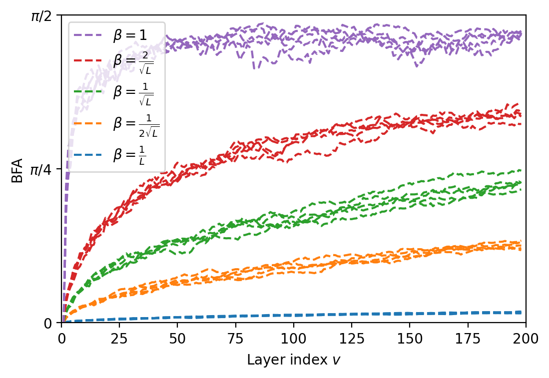
(a) BFA vs. layer ($L=200$)

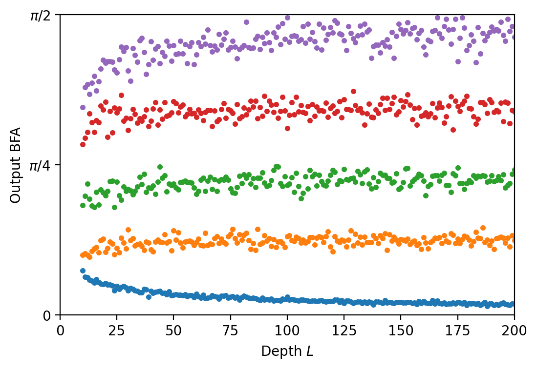
(b) Output BFA vs. depth

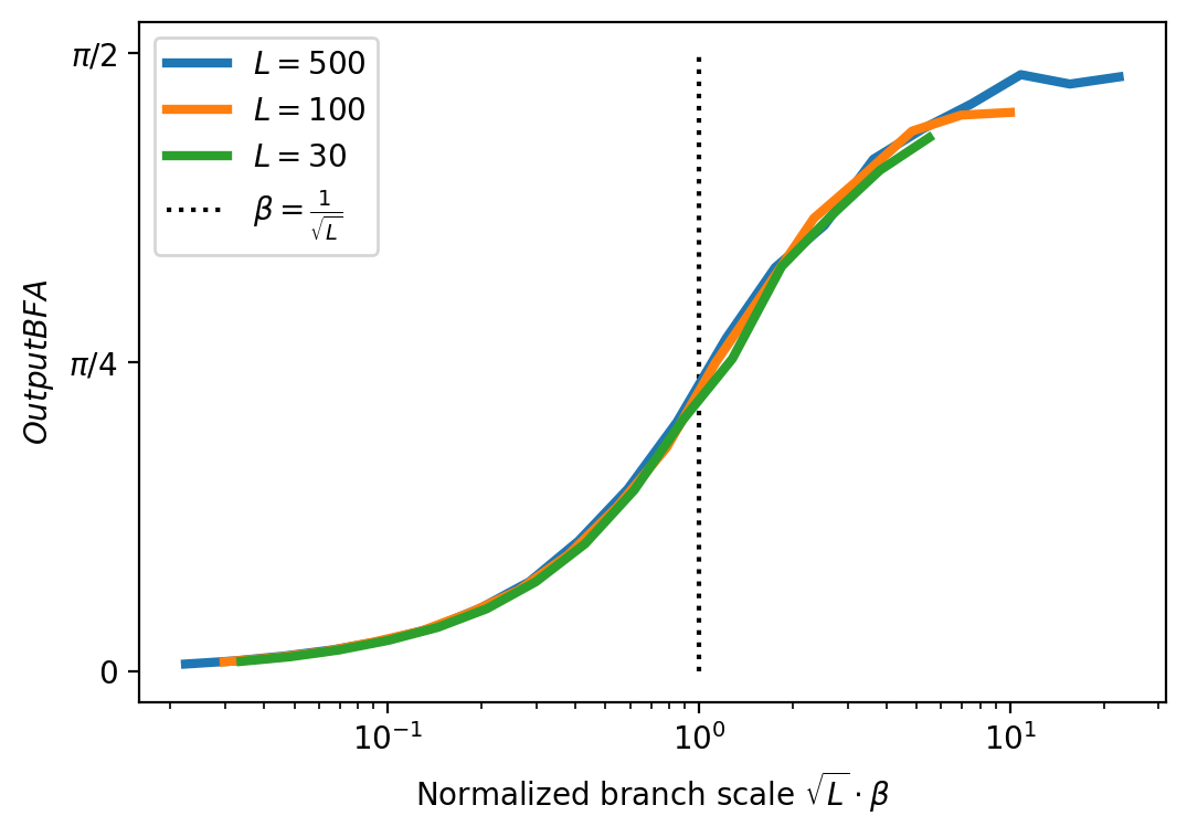
(c) Output BFA vs. scale

Figure 4: Backward-Feature Angle (BFA) $\widehat{b_{v},\delta f_{v}}$ observed at initialization in MLPs and ResNets (witdh $m=200$), for a few random realizations. (a) for all architectures, BFA varies in the first few layers and then stabilizes. (b) BFA at output layer is asymptotically independent of depth, with a non-trivial angle only when $\beta\propto\nicefrac{{1}}{{\sqrt{L}}}$ (same color scheme as (a)). (c) for a branch scale $\beta=\nicefrac{{c}}{{\sqrt{L}}}$, the factor $c$ directly determines asymptotic output BFA (averaged over $5$ draws).

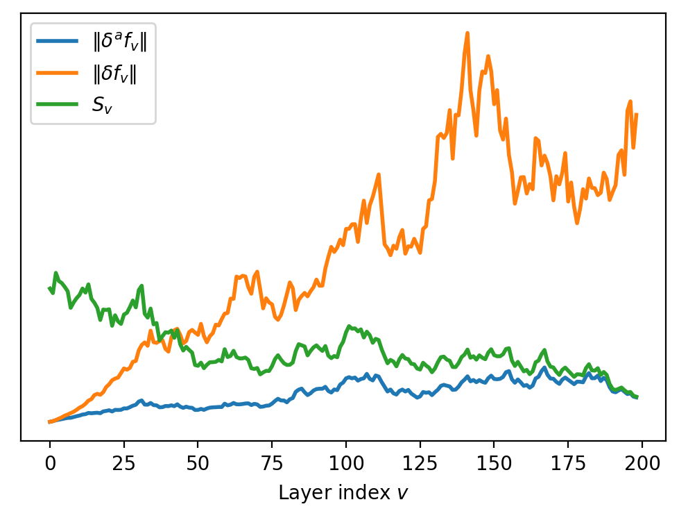
(a) MLP ($\beta=1$)

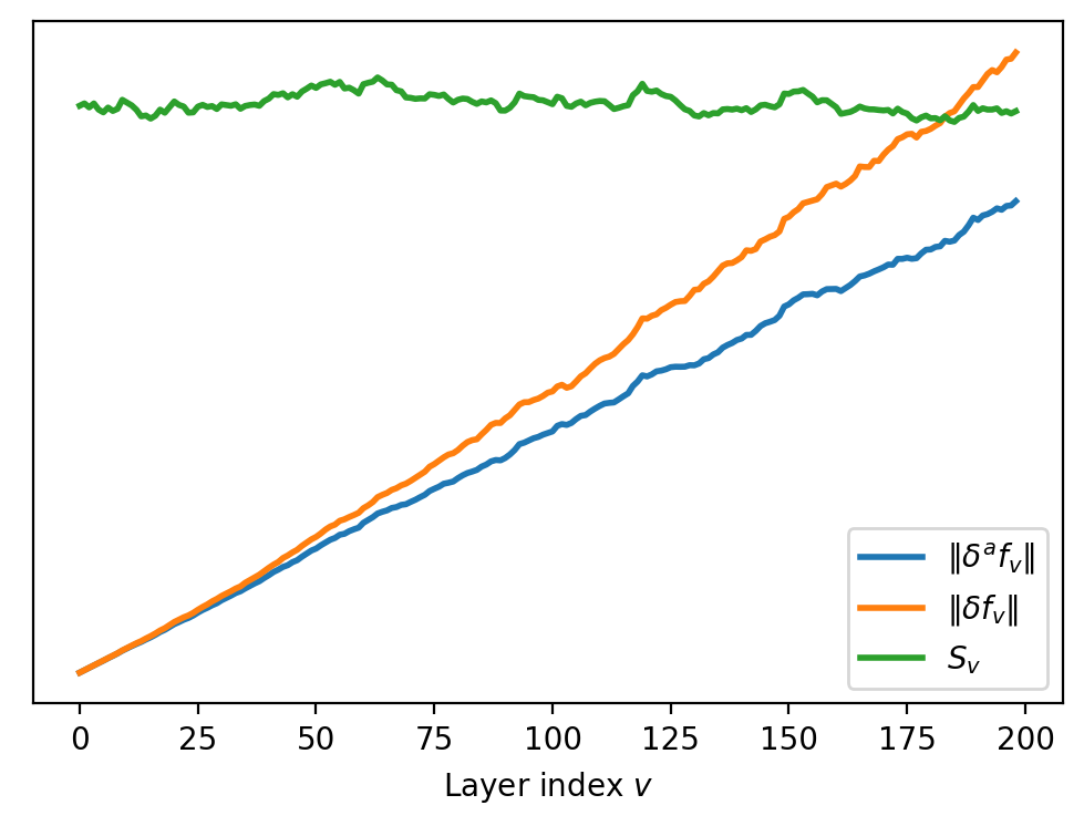
(b) ResNet with $\beta=\nicefrac{{1}}{{\sqrt{L}}}$

Figure 5: Magnitudes of feature updates $\|\delta f_{v}\|_{\mathrm{rms}}/\eta_{0}$, BAFU $\|\delta^{\mathrm{a}}f_{v}\|_{\mathrm{rms}}/\eta_{0}$ and sensitivities $S_{v}$ as a function of layer index, in a randomly initialized (a) MLP and (b) ResNet (criterion (C) is enforced in both). These quantities are random and we show a typical draw. (a) In a MLP, finite width effects make the sensitivities vary wildly which makes it difficult to control BAFU, and a fortiori feature updates (since alignment degenerates as well). (b) In a ResNet, all the quantities are well-behaved and all criteria/desiderata are satisfied.

5 Conclusion

By introducing the notion of alignment between feature update and backward pass, we have divided the difficult problem of studying feature learning in two parts: (i) the study of alignment, which can be done theoretically (at initialization) or empirically, and (ii) the study of BAFU, which involves the very general BAFU formula and its consequences. Together, these tools allow to predict, measure and control feature learning.

In this paper, our goal was to introduce the framework and derive its first consequences. We believe that many questions are yet to be answered, both from a practical and theoretical point of view. Examples of such questions are: from a practical point of view, what are the behaviors for the universal HP from FSC that lead to the best performances ? From a theoretical point of view, can we exactly characterize alignment for certain architectures ?

Acknowledgments.

We thank Loucas Pillaud-Vivien for inspiring discussions and feedback.

Appendix A Alignment and BAFU in general architectures

In this section, we continue using $\|\cdot\|_{2}$ for the $\ell_{2}$, or Frobenius norm of a tensor, and $\|\cdot\|_{\mathrm{rms}}$ for its RMS-norm.

A.1 Gradient update in a general architecture

Forward pass.

There are several levels of granularity to represent the forward pass as a computational graph. The one that is convenient to us is when each symbolic variable is a matrix. We thus consider $\mathcal{G}=(\mathcal{V},\mathcal{E})$ a directed acyclic graph (DAG) of size $V$ with vertices $\mathcal{V}\coloneqq\{1,2,\dots,V\}$ indexed by a (fixed) topological ordering. Given a node $v\in\mathcal{V}$, we denote by $\mathrm{pa}(v)$ its parents. Each node $v$ (referred to as a feature node) is associated to a symbolic variable $F_{v}\in\mathbb{R}^{m_{v}\times n_{v}}$ which stands for an intermediate computation in the forward pass and we assume that there is a unique sink that stands for the loss $\mathcal{L}\coloneqq F_{V}\in\mathbb{R}$. Here $m_{v}$ stands for the dimension along which matrix multiplication acts, and $n_{v}$ the product of all other dimensions (typically batch-size, or context length in attention blocks). Starting from the input variables $\{F_{1},\dots F_{V_{0}}\}$ (where $\{1,\dots,V_{0}\}$ are the nodes satisfying $\mathrm{pa}(v)=\emptyset$), new variables are computed from previous ones via

$$F_{v}=T_{v}(F_{\mathrm{pa}(v)}).$$

where $T_{v}$ is a (potentially parameterized or non-differentiable) map.

We denote by $\mathcal{W}\subset\mathcal{V}$ the subset of nodes that directly follow matrix product against a trainable weight matrix $W_{\ell}$. Such a node $\ell\in\mathcal{W}$ (referred to as a weight node) must have a unique parent (i.e. $\#\mathrm{pa}(\ell)=1$) that we denote by $\ell^{-}$, the sizes must be compatible (i.e. $n_{\ell}=n_{\ell^{-}}$ and $W_{\ell}\in\mathbb{R}^{m_{\ell}\times m_{\ell^{-}}}$) and we have

$$F_{\ell}=T_{\ell}(F_{\ell^{-}};W_{\ell})\coloneqq W_{\ell}F_{\ell^{-}}.$$

We assume that each weight matrix is only used once in the forward pass (this excludes recurrent architectures from our analysis). The computation of the forward pass is given in Algorithm 1.

Backward pass.

The gradient of $\mathcal{L}$ with respect to the weights $(W_{\ell})_{\ell\in\mathcal{W}}$, is computed with the back-propagation algorithm given in Algorithm 2. It recursively defines a family of variables $B_{v}\in\mathbb{R}^{m_{v}\times n_{v}}$ that correspond to the symbolic gradients $B_{v}=\big{(}\frac{\partial\mathcal{L}}{\partial F_{v}}\big{)}^{*}$. For $v^{\prime}\in\mathrm{pa}(v)$, we denote the partial Jacobian of $T_{v}$ by

$$J_{v^{\prime}\to v}\coloneqq\frac{\partial F_{v}}{\partial F_{v^{\prime}}}$$

which is a linear operator $\mathbb{R}^{m_{v^{\prime}}\times n_{v^{\prime}}}\to\mathbb{R}^{m_{v}\times n_{v}}$, whose adjoint we denote by $J_{v^{\prime}\to v}^{*}$ (it depends on the forward pass although this is not recalled in our notation). Finally the weight update, for $\ell\in\mathcal{W}$, is

$$\delta W_{\ell}=-\eta_{\ell}B_{\ell}F_{\ell^{-}}^{\top}.$$

where $\eta_{\ell}>0$ is the layer-wise learning-rate. Note that in Algorithm 2, the computation of $B_{v}$ for $v\in\{1,\dots,V_{0}\}$ is not needed for the weights updates and can be skipped.

Path Jacobian

A path of length $K$ joining $v_{1}$ to $v_{K+1}$ in the graph $\mathcal{G}$ is a tuple $\xi=((v_{1},v_{2}),\dots,(v_{L},v_{K+1}))$ where each $(v_{i},v_{i+1})$ is an oriented edge of $\mathcal{G}$. Given a path $\xi$, we define the path Jacobian $J_{\xi}$ as

$$J_{\xi}=J_{v_{L}\to v_{K+1}}\circ\dots\circ J_{v_{1}\to v_{2}}.$$

This is a linear operator from $\mathbb{R}^{m_{1}\times n_{1}}$ to $\mathbb{R}^{m_{K+1}\times n_{K+1}}$. For any pair of vertices $v,v^{\prime}\in\mathcal{V}$, let $\mathcal{P}(v,v^{\prime})$ the set of paths between them and let

$$J_{v\to v^{\prime}}=\sum_{\xi\in\mathcal{P}(v,v^{\prime})}J_{\xi}$$ (22)

which coincides with the derivative $\frac{\partial F_{v^{\prime}}}{\partial F_{v}}$.

Input: $F_{1},\dots,F_{V_{0}}$

For $v=V_{0}+1,\dots,V$:

 $F_{v}=T_{v}(F_{\mathrm{pa}(v)})$

Output: $(F_{v})_{v\in\mathcal{V}}$

Algorithm 1 Forward pass

Input: $B_{V}\coloneqq 1$, $B_{v}\coloneqq 0$, for $v\neq V$

For $v=V,\dots,1$:

 For $v^{\prime}\in\mathrm{pa}(v)$:

  $B_{v^{\prime}}=B_{v^{\prime}}+J_{v^{\prime}\to v}^{*}(B_{v})$

Output: $(B_{v})_{v\in\mathcal{V}}$

Algorithm 2 Backward pass

Figure 6: (left) Forward pass to compute the loss on a batch (the trainable weight matrices are implicit). (right) Backward pass, given by the backpropagation algorithm.

Illustrative example

As a simple example, we plot on Fig. 7 the computational graph for the loss (forward pass) of a $2$-layer MLP with intercept and residual connections on a batch of size $n$. For equal input, hidden and output widths $m$, the trainable parameters are the weights matrices $W_{3},W_{6}\in\mathbb{R}^{m\times m}$ and the intercepts $W_{4},W_{8}\in\mathbb{R}^{m}$. To compute the loss for a batch of $n$ inputs of dimension $m$ stored in a matrix $X\in\mathbb{R}^{m\times n}$, we first assign $F_{1}=X\in\mathbb{R}^{m\times n}$ and $F_{2},F_{6}=(1,\dots,1)\in\mathbb{R}^{1\times n}$ and then performs the following computations:

$$F_{3} =W_{3}F_{1}\in\mathbb{R}^{m\times n}, F_{4} =W_{4}F_{2}\in\mathbb{R}^{m\times n}, F_{5} =T_{5}(F_{1},F_{3},F_{4})\in\mathbb{R}^{m\times n}$$ (23)

$$F_{7} =W_{6}F_{5}\in\mathbb{R}^{k\times n}, F_{8} =W_{8}F_{6}\in\mathbb{R}^{m\times n}, F_{9} =T_{9}(F_{5},F_{7},F_{8})\in\mathbb{R}$$ (24)

where there are two “untrained” maps, defined as

$$T_{5}(F_{1},F_{3},F_{4}) \coloneqq\phi(F_{1}+F_{3}+F_{4}), T_{9}(F_{5},F_{7},F_{8})\coloneqq\frac{1}{mn}\|F_{5}+F_{7}+F_{8}-Y\|_{2}^{2}$$

and $\phi:\mathbb{R}\to\mathbb{R}$ is the activation function acting entry-wise (such as ReLU) and here we have used the square loss with respect to output data $Y\in\mathbb{R}^{m\times n}$. In particular, our framework allows to include intercepts/biases by introducing some dummy inputs $F_{2}$ and $F_{6}$. In what follows we develop tools to quantify the influence of the weights updates (in red) on the features (in blue).

Figure 7: Illustration of our notation with the forward pass of a two-layer neural network with intercepts and residual connections (toy model).

A.2 Aligned Updates Formula in the general case

In this general setting, the definition of feature updates and their projection on the backward pass reads as follows.

Definition A.1 (Backward-Aligned Feature Update (BAFU)).

Let $v\in\mathcal{V}$ a feature node and $\ell\in\mathcal{W}$ a weight node. If there exists a path from $\ell$ to $v$, the partial feature update of $F_{v}$ due to the weight matrix $W_{\ell}$ is defined as

$$\delta_{\ell}F_{v}\coloneqq-\eta_{\ell}J_{\ell\to v}(B_{\ell}F_{\ell^{-}}^{\top}F_{\ell^{-}})$$

and by $\delta_{\ell}F_{v}\coloneqq 0$ otherwise. The partial BAFU $\delta_{\ell}^{\mathrm{a}}F_{v}$ is defined as the projection of $\delta_{\ell}F_{v}$ on the span of $B_{v}$, that is if $\delta_{\ell}F_{v}\neq 0$,

$$\delta_{\ell}^{\mathrm{a}}F_{v}\coloneqq\frac{\langle B_{v},\delta_{\ell}F_{v}\rangle_{2}}{\|B_{v}\|^{2}_{2}}B_{v}.$$

Finally, the feature update, resp. BAFU, are defined as

$$\delta F_{v}=\sum_{\ell\in\mathcal{W}}\delta_{\ell}F_{v}, \delta^{\mathrm{a}}F_{v}=\sum_{\ell\in\mathcal{W}}\delta_{\ell}^{\mathrm{a}}F_{v}.$$

Definition A.2 (Contributions & Sensitivities).

For a weight node $\ell\in\mathcal{W}$, its contribution is defined as

$$C_{\ell}\coloneqq\eta_{\ell}\|\nabla_{\ell}\|^{2}_{2}=-\eta_{\ell}\operatorname{tr}(F_{\ell_{-}}B_{\ell}^{\top}B_{\ell}F_{\ell_{-}}^{\top}).$$

where $\nabla_{\ell}\coloneqq\nabla_{\ell}\mathcal{L}$. For a feature node $v\in\mathcal{V}$, its sensitivity is defined as

$$S_{v}\coloneqq\big{(}\sqrt{s_{v}}\cdot\|B_{v}\|_{2}\big{)}^{-1}=\big{(}s_{v}\cdot\|B_{v}\|_{\mathrm{rms}}\big{)}^{-1}$$

where $s_{v}=m_{v}\cdot n_{v}$ is the total number of entries in $F_{v}$ (or equivalently, in $B_{v}$).

Definition A.3 (Graph properties).

Consider the computational graph of the forward pass of a NN with nodes $\mathcal{V}$.

• For $\ell,v\in\mathcal{V}$, we say that $v$ separates $\ell$ from the loss if any path from $\ell$ to the loss contains $v$.

• For $v\in\mathcal{V}$, let $\mathcal{W}_{v}\subset\mathcal{W}$ be the set of weight matrices $\ell$ such that there exists a path from $\ell$ to $v$. We say that $v$ is a cut node if $\forall\ell\in\mathcal{W}_{v}$, $v$ separates $\ell$ from the loss.

Let us stress that Eq. (25) applies also to couples of the form $(v,v)$, that is (by convention) $v$ separates $v$ from the loss. As an illustration, in the computational graph shown on Fig. 7, Eq. (25) can be applied to the pairs $(W_{3},F_{3})$ $(W_{6},F_{7})$ and $(W_{4},F_{5})$ (among others). As for Eq. (26), it is valid for all nodes (i.e. all nodes are cut nodes) except $F_{7}$.

Proof.

Under our assumptions, the negative dot-product between $\delta_{\ell}F_{v}$ and $B_{v}$ writes

$$-\langle B_{v},\delta_{\ell}F_{v}\rangle_{2} =\eta_{\ell}\langle B_{v},J_{\ell\to v}(B_{\ell}F_{\ell^{-}}^{\top}F_{\ell^{-}})\rangle_{2}$$

$$\overset{(i)}{=}\eta_{\ell}\langle J^{*}_{\ell\to v}(B_{v}),B_{\ell}F_{\ell^{-}}^{\top}F_{\ell^{-}}\rangle_{2}$$

$$\overset{(ii)}{=}\eta_{\ell}\langle B_{\ell},B_{\ell}F_{\ell^{-}}^{\top}F_{\ell^{-}}\rangle_{2}$$

$$\overset{(iii)}{=}\eta_{\ell}\operatorname{tr}(B_{\ell}^{\top}B_{\ell}F_{\ell^{-}}^{\top}F_{\ell^{-}})$$

$$\overset{(iv)}{=}\eta_{\ell}\operatorname{tr}(F_{\ell^{-}}B_{\ell}^{\top}B_{\ell}F_{\ell^{-}}^{\top})=C_{\ell}\geq 0$$

where we have used (i) the definition of adjoint operator, (ii) Lemma A.5 below (this is where the graph property is needed), (iii) the definition of $\langle\cdot,\cdot\rangle_{2}$ for matrices and (iv) the invariance of the trace under cyclic permutations. Thus it holds

$$\|\delta_{w}^{\mathrm{al}}F_{v}\|_{2}=-\frac{\langle B_{v},\delta_{\ell}F_{v}\rangle_{2}}{\|B_{v}\|_{2}}=\frac{C_{\ell}}{\|B_{v}\|_{2}}$$

and Eq. (25) follows by converting into RMS-norm. Finally, since we have proved $-\operatorname{tr}(B_{v}^{\top}\delta_{\ell}F_{v})=C_{\ell}\geq 0$ for all $\ell\in\mathcal{W}_{v}$, we have

$$\Big{\|}\sum_{\ell\in\mathcal{W}_{v}}\delta_{\ell}^{\mathrm{al}}F_{v}\Big{\|}_{2}=\sum_{\ell\in\mathcal{W}_{v}}\big{\|}\delta_{\ell}^{\mathrm{al}}F_{v}\big{\|}_{2}$$

and Eq. 26 follows. ∎

Lemma A.5 (A generalized chain rule).

If $v$ separates $\ell$ from the loss, then $B_{\ell}=J^{*}_{\ell\to v}(B_{v})$.

Proof.

Using the definition of path Jacobian and from the backpropagation algorithm, we have that

$$B_{\ell}=\sum_{\xi\in\mathcal{P}(\ell,V)}J_{\xi}^{*}(1)$$

where $\mathcal{P}(\ell,V)$ is the set of paths from $w$ to the loss node $V$. Thanks to the condition on $v$, any path in $\mathcal{P}(\ell,V)$ can be uniquely factored as $\xi=(\xi_{a},\xi_{b})$ where $\xi_{a}$ is a path from $\ell$ to $v$ and $\xi_{b}$ is a path from $v$ to the loss. This leads to the decomposition

$$B_{\ell}=\sum_{\xi_{a}\in\mathcal{P}(\ell,v)}\sum_{\xi_{b}\in\mathcal{P}(v,V)}(J_{\xi_{a}}^{*}\circ J_{\xi_{b}}^{*})(1)=\Big{(}\sum_{\xi_{a}\in\mathcal{P}(\ell,v)}J_{\xi_{a}}^{*}\Big{)}\circ\Big{(}\sum_{\xi_{b}\in\mathcal{P}(v,V)}J_{\xi_{b}}^{*}(1)\Big{)}=J^{*}_{\ell\to v}(B_{v}).\qed$$

A.3 Alignment in the general case: Backward to Feature Kernel

In the general case, the Backward to Feature Kernel (BFK), is defined as follows.

Definition A.6 (Backward to Feature Kernel).

For a pair $(\ell,v)\in\mathcal{W}\times\mathcal{V}$ such that there exists a path from $\ell$ to $v$, the partial BFK $\mathcal{K}_{\ell\to v}$ is a self linear map on $\mathbb{R}^{m_{v}\times n_{v}}$ defined as

$$\mathcal{K}_{\ell\to v}(B)=\eta_{\ell}J_{\ell\to v}(J_{\ell\to v}^{*}(B)F_{\ell^{-}}^{\top}F_{\ell^{-}}).$$

Then for $v\in\mathcal{V}$, the (total) BFK is defined as

$$\mathcal{K}_{v}=\sum_{\ell\in\mathcal{W}_{v}}\mathcal{K}_{\ell\to v}.$$

This operator $\mathcal{K}_{v}$ describes how a neural network transforms a given backward pass $B_{v}$ at a node $v\in\mathcal{V}$ into an update for the feature $F_{v}$, in the small step-size limit. Clearly, $\mathcal{K}_{\ell\to v}$ are self-adjoint positive semidefinite (psd) operators – and hence $\mathcal{K}_{v}$ as well – since for any $A,B\in\mathbb{R}^{m_{v}\times n_{v}}$,

$$\langle A,\mathcal{K}_{\ell\to v}(B)\rangle_{2} =\eta_{\ell}\langle J_{\ell\to v}^{*}(A),J_{\ell\to v}^{*}(B)F_{\ell^{-}}^{\top}F_{\ell^{-}}\rangle_{2}$$

$$=\eta_{\ell}\langle J_{\ell\to v}^{*}(A)F_{\ell^{-}}^{\top},J_{\ell\to v}^{*}(B)F_{\ell^{-}}^{\top}\rangle_{2}$$

$$=\langle\Phi(A),\Phi(B)\rangle_{2}$$

where in the intermediate step we have used that $\langle A,BC\rangle=\operatorname{tr}(A^{\top}BC)=\operatorname{tr}(CA^{\top}B)=\operatorname{tr}((AC^{\top})^{\top}B)=\langle AC^{\top},B\rangle$, and we define the feature map

$$\Phi(A)\coloneqq\sqrt{\eta_{\ell}}J^{*}_{\ell\to v}(A)F_{\ell^{-}}^{\top}\in\mathbb{R}^{m_{\ell}\times m_{\ell^{-}}}.$$

In particular, this operator admits an orthonormal basis of eigenvectors and all its eigenvalues are real nonnegative. Several particular cases of this operator are well known:

• (Loss decrease). When $v=V$ is the loss node, then $m_{V}=n_{V}=1$ and $J_{\ell\to V}=\operatorname{tr}(B_{\ell}^{\top}\cdot)$. Hence for a scalar $B=1\in\mathbb{R}$,

  $$\mathcal{K}_{\ell\to V}(1) =\eta_{\ell}\operatorname{tr}(B_{\ell}^{\top}B_{\ell}F_{\ell^{-}}^{\top}F_{\ell^{-}})=C_{\ell} \mathcal{K}_{V}(1)=\sum_{\ell\in\mathcal{W}}C_{\ell}=\delta\mathcal{L}.$$ and

  Hence $\mathcal{K}_{V}(1)$ is simply the change of loss after one gradient step.

• (Gramian of the Jacobian) In case $n_{v}=1$ (e.g. MLP with batch size $1$) then $\mathcal{K}_{\ell\to v}$ is proportional to $J_{\ell\to v}J^{\top}_{\ell\to v}$. This is the case studied in the main text.

• (Neural Tangent Kernel). In the common setting of regression or binary classification, the penultimate forward variable $F_{\text{out}}$ with $\text{out}=V-1$ is the concatenation of $n=n_{v_{0}}$ scalar predictions $(f(x_{1}),\dots,f(x_{n}))$ which are the logit/predictions associated the inputs $(x_{1},\dots,x_{n})\in(\mathbb{R}^{d})^{n}$. In this case, $\mathcal{K}_{\text{out}}$ is the usual notion of neural tangent kernel [Jacot et al., 2018]. Indeed, denoting $e_{i}\in\mathbb{R}^{n}$ the $i$-th vector from the canonical basis, it holds $J^{*}_{\ell\to\text{out}}(e_{i})=\tilde{B}(x_{i})e_{i}^{\top}$ where $\tilde{B}(x_{i})\coloneqq\big{(}\frac{\partial f(x_{i})}{\partial F_{\ell}}\big{)}^{*}$. Now let us denote $\tilde{F}_{i}\coloneqq F_{\ell^{-}}e_{i}\in\mathbb{R}^{m_{\ell^{-}}}$ the feature at node $\ell^{-}$ restricted to the input $x_{i}$. Then the partial kernel matrix has entries

  $$K^{(\ell)}_{i,j} \coloneqq\langle e_{i},\mathcal{K}_{\ell\to\text{out}}(e_{j})\rangle$$

  $$=\eta_{\ell}\langle J^{*}_{\ell\to\text{out}}(e_{i})F_{\ell^{-}}^{\top},J^{*}_{\ell\to\text{out}}(e_{j})F_{\ell^{-}}^{\top}\rangle$$

  $$=\eta_{\ell}\operatorname{tr}(F_{\ell^{-}}e_{i}\tilde{B}(x_{i})^{\top}\tilde{B}(x_{j})e_{j}^{\top}F_{\ell^{-}}^{\top})$$

  $$=\eta_{\ell}\operatorname{tr}(\tilde{F}(x_{i})\tilde{B}(x_{i})^{\top}\tilde{B}(x_{j})\tilde{F}(x_{j})^{\top})$$

  $$=\eta_{\ell}\langle\nabla_{W_{\ell}}f(x_{i}),\nabla_{W_{\ell}}f(x_{j})\rangle$$

  which is the definition of the partial tangent kernel with respect to layer $\ell$. Thus $\mathcal{K}_{\text{out}}$, as the sum of these partial kernels, is exactly the Neural Tangent Kernel. Here again, its spectrum is a well-studied object, e.g. [Bietti and Bach, 2021, Fan and Wang, 2020], which can also be obtained by studying the Fisher-Information operator [Karakida et al., 2019].

General alignment

Let us finally show that the difference between the aligned and full feature updates magnitude is directly captured in terms of the BFK. In this generalization of Prop. 2.6, we denote by $\mathcal{K}^{\nicefrac{{1}}{{2}}}$ the unique psd square-root of a psd operator $\mathcal{K}$.

Proposition A.7 (Alignment and BFK).

If $v$ separates $\ell$ from the loss then

$$\delta_{\ell}F_{v}=-\mathcal{K}_{\ell\to v}(B_{v}), \|\delta^{\mathrm{a}}_{\ell}F_{v}\|_{2}=\frac{\|\mathcal{K}_{\ell\to v}^{\nicefrac{{1}}{{2}}}(B_{v})\|_{2}^{2}}{\|B_{v}\|_{2}}$$ and

Moreover, if $v$ is a cut node then

$$\delta F_{v}=-\mathcal{K}_{v}(B_{v}), \|\delta^{\mathrm{a}}F_{v}\|_{2}=\frac{\|\mathcal{K}_{v}^{\nicefrac{{1}}{{2}}}(B_{v})\|_{2}^{2}}{\|B_{v}\|_{2}}$$ and (27)

Proof.

If $v$ separates $\ell$ from the loss then by Lem. A.5, $B_{\ell}=J^{*}_{\ell\to v}(B_{v})$. It follows, on the one hand,

$$\mathcal{K}_{\ell\to v}(B_{v})=\eta_{\ell}J_{\ell\to v}(J_{\ell\to v}^{*}(B_{v})F_{\ell^{-}}^{\top}F_{\ell^{-}})=\eta_{\ell}J_{\ell\to v}(B_{\ell}F_{\ell^{-}}^{\top}F_{\ell^{-}})=-\delta_{\ell}F_{v},$$

and on the other hand

$$\|\delta^{\mathrm{a}}_{\ell}F_{v}\|_{2}=\frac{\langle B_{v},\mathcal{K}_{\ell\to v}(B_{v})\rangle_{2}}{\|B_{v}\|_{2}}=\frac{\langle\mathcal{K}^{\nicefrac{{1}}{{2}}}_{\ell\to v}(B_{v}),\mathcal{K}^{\nicefrac{{1}}{{2}}}_{\ell\to v}(B_{v})\rangle_{2}}{\|B_{v}\|_{2}}=\frac{\|\mathcal{K}_{\ell\to v}^{\nicefrac{{1}}{{2}}}(B_{v})\|_{2}^{2}}{\|B_{v}\|_{2}}.$$

The proof is analogous for the total (aligned) feature update. ∎

Appendix B Characterization of reparameterization invariant LR

Consider a function $f:\prod_{\ell=1}^{L}\mathbb{R}^{p_{\ell}}\to\mathbb{R}$ admitting a (selection) derivative and, for a fixed scale vector $\alpha\in(\mathbb{R}^{*}_{+})^{L}$ consider the function $g(y)=f(\alpha\cdot y)$ where $\alpha\cdot x$ denotes $(\alpha_{1}x_{1},\dots,\alpha_{L}x_{L})$. Consider one step of GD on the two functions, given for $\ell\in[1:L]$, by

$$x^{\prime}_{\ell} =x_{\ell}-\eta_{\ell}\nabla_{\ell}f(x)$$

$$y^{\prime}_{\ell} =y_{\ell}-\eta_{\ell}\nabla_{\ell}g(y)$$

with identical starting points, that is $x_{\ell}=\alpha_{\ell}\cdot y_{\ell}$ for $\ell\in[1:L]$.

Proposition B.1.

Consider adaptive learning rates, which are of the form $\eta_{\ell}=\eta_{\ell}(\nabla f(x))$. Then $x^{\prime}=\alpha\cdot y^{\prime}$ for all $\alpha\in(\mathbb{R}^{*}_{+})^{L}$ if and only if $\eta_{\ell}$ is $(-2)$-homogeneous in $\nabla_{\ell}f(x)$ and $0$-homogeneous in $\nabla_{\ell^{\prime}}f(x)$ for $\ell\neq\ell^{\prime}$.

The most natural choice of such a learning rate is precisely the learning rate suggested by the (C) criterion $\eta_{\ell}\propto\|\nabla_{\ell}f(x)\|_{2}^{-2}$.

Proof.

For $\ell\in[1:L]$, it holds

$$\alpha_{\ell}y^{\prime}_{\ell} =\alpha_{\ell}y_{\ell}-\alpha_{\ell}\eta_{\ell}(\nabla g(y))\nabla_{\ell}g(y)$$

$$=x_{\ell}-\alpha_{\ell}^{2}\eta_{\ell}(\alpha\cdot\nabla f(x))\nabla_{\ell}f(x).$$

Then $\alpha\cdot y^{\prime}=x^{\prime}$ for all $\alpha\in(\mathbb{R}^{*}_{+})^{L}$ is equivalent to

$$\alpha_{\ell}^{2}\eta_{\ell}(\alpha\cdot\nabla f(x))=\eta_{\ell}(\nabla f(x)),\quad\forall\alpha\in(\mathbb{R}^{*}_{+})^{L}$$

which is exactly the claimed homogeneity property. ∎

Appendix C Computations of alignment

We consider the context of Section 4.1. By Prop. 2.6 we have

$$\cos(\widehat{b_{v},\delta f_{v}})\geq\left(\frac{1}{v}\sum_{\bar{\ell}\leq v}\frac{\sqrt{M^{(2)}_{\bar{\ell}\to v}}}{M^{(1)}_{\bar{\ell}\to v}}\right)^{-1}.$$

For simplicity, we replace $M^{(p)}_{\bar{\ell}\to v}$ by $M^{(1)}_{\ell\to v}$ as this does not change the asymptotic behavior for $v-\ell$ large. By 4.1 we have for $v\gg 1$,

$$\frac{1}{v}\sum_{\ell\leq v}\frac{\sqrt{M^{(2)}_{\ell\to v}}}{M^{(1)}_{\ell\to v}}=\frac{1}{v}\sum_{\ell=1}^{v}\sqrt{2\ell+1}\sim\frac{1}{v}\int_{0}^{v}\sqrt{2x+1}\mathrm{d}x=\frac{1}{v}\frac{2}{3}\frac{(2v+1)^{3/2}}{2}\sim\frac{\sqrt{8v}}{3}.$$

References

• Allen-Zhu et al. [2019] Zeyuan Allen-Zhu, Yuanzhi Li, and Zhao Song. A convergence theory for deep learning via over-parameterization. In International conference on machine learning, pages 242–252. PMLR, 2019.
• Atanasov et al. [2021] Alexander Atanasov, Blake Bordelon, and Cengiz Pehlevan. Neural networks as kernel learners: The silent alignment effect. In International Conference on Learning Representations, 2021.
• Baratin et al. [2021] Aristide Baratin, Thomas George, César Laurent, R Devon Hjelm, Guillaume Lajoie, Pascal Vincent, and Simon Lacoste-Julien. Implicit regularization via neural feature alignment. In International Conference on Artificial Intelligence and Statistics, pages 2269–2277. PMLR, 2021.
• Bietti and Bach [2021] Alberto Bietti and Francis Bach. Deep equals shallow for ReLU networks in kernel regimes. In ICLR 2021-International Conference on Learning Representations, pages 1–22, 2021.
• Bolte and Pauwels [2020] Jérôme Bolte and Edouard Pauwels. A mathematical model for automatic differentiation in machine learning. Advances in Neural Information Processing Systems, 33:10809–10819, 2020.
• Bordelon et al. [2023] Blake Bordelon, Lorenzo Noci, Mufan Bill Li, Boris Hanin, and Cengiz Pehlevan. Depthwise hyperparameter transfer in residual networks: Dynamics and scaling limit. arXiv preprint arXiv:2309.16620, 2023.
• Chizat and Bach [2018] Lénaïc Chizat and Francis Bach. On the global convergence of gradient descent for over-parameterized models using optimal transport. Advances in Neural Information Processing Systems, 31, 2018.
• Chizat et al. [2019] Lénaic Chizat, Edouard Oyallon, and Francis Bach. On lazy training in differentiable programming. Advances in Neural Information Processing Systems, 32, 2019.
• Du et al. [2018] Simon S Du, Xiyu Zhai, Barnabas Poczos, and Aarti Singh. Gradient descent provably optimizes over-parameterized neural networks. In International Conference on Learning Representations, 2018.
• Duchi et al. [2011] John Duchi, Elad Hazan, and Yoram Singer. Adaptive subgradient methods for online learning and stochastic optimization. Journal of machine learning research, 12(7), 2011.
• Fan and Wang [2020] Zhou Fan and Zhichao Wang. Spectra of the conjugate kernel and neural tangent kernel for linear-width neural networks. Advances in Neural Information Processing Systems, 33:7710–7721, 2020.
• Golikov and Yang [2022] Eugene Golikov and Greg Yang. Non-gaussian tensor programs. Advances in Neural Information Processing Systems, 35:21521–21533, 2022.
• Hanin [2018] Boris Hanin. Which neural net architectures give rise to exploding and vanishing gradients? Advances in neural information processing systems, 31, 2018.
• Hanin and Nica [2020] Boris Hanin and Mihai Nica. Products of many large random matrices and gradients in deep neural networks. Communications in Mathematical Physics, 376(1):287–322, 2020.
• Hanin and Rolnick [2018] Boris Hanin and David Rolnick. How to start training: The effect of initialization and architecture. Advances in Neural Information Processing Systems, 31, 2018.
• Hayou et al. [2021] Soufiane Hayou, Eugenio Clerico, Bobby He, George Deligiannidis, Arnaud Doucet, and Judith Rousseau. Stable ResNet. In International Conference on Artificial Intelligence and Statistics, pages 1324–1332. PMLR, 2021.
• Hazan and Kakade [2019] Elad Hazan and Sham Kakade. Revisiting the Polyak step size. arXiv preprint arXiv:1905.00313, 2019.
• Jacot et al. [2018] Arthur Jacot, Franck Gabriel, and Clément Hongler. Neural Tangent Kernel: Convergence and generalization in neural networks. Advances in Neural Information Processing Systems, 31, 2018.
• Jelassi et al. [2023] Samy Jelassi, Boris Hanin, Ziwei Ji, Sashank J Reddi, Srinadh Bhojanapalli, and Sanjiv Kumar. Depth dependence of $\mu$-P learning rates in ReLU MLPs. arXiv preprint arXiv:2305.07810, 2023.
• Karakida et al. [2019] Ryo Karakida, Shotaro Akaho, and Shun-ichi Amari. Universal statistics of Fisher information in deep neural networks: Mean field approach. In The 22nd International Conference on Artificial Intelligence and Statistics, pages 1032–1041. PMLR, 2019.
• Kingma and Ba [2015] Diederik Kingma and Jimmy Ba. Adam: A method for stochastic optimization. In International Conference on Learning Representations (ICLR), San Diega, CA, USA, 2015.
• LeCun et al. [2015] Yann LeCun, Yoshua Bengio, and Geoffrey Hinton. Deep learning. Nature, 521(7553):436–444, 2015.
• Li et al. [2021] Mufan Li, Mihai Nica, and Dan Roy. The future is log-Gaussian: ResNets and their infinite-depth-and-width limit at initialization. Advances in Neural Information Processing Systems, 34:7852–7864, 2021.
• Li et al. [2022] Zhiyuan Li, Srinadh Bhojanapalli, Manzil Zaheer, Sashank Reddi, and Sanjiv Kumar. Robust training of neural networks using scale invariant architectures. In International Conference on Machine Learning, pages 12656–12684. PMLR, 2022.
• Ling and Qiu [2019] Zenan Ling and Robert C. Qiu. Spectrum concentration in deep residual learning: a free probability approach. IEEE Access, 7:105212–105223, 2019.
• Lou et al. [2022] Yizhang Lou, Chris E Mingard, and Soufiane Hayou. Feature learning and signal propagation in deep neural networks. In International Conference on Machine Learning, pages 14248–14282. PMLR, 2022.
• Marion et al. [2022] Pierre Marion, Adeline Fermanian, Gérard Biau, and Jean-Philippe Vert. Scaling ResNets in the large-depth regime. arXiv preprint arXiv:2206.06929, 2022.
• Mei et al. [2018] Song Mei, Andrea Montanari, and Phan-Minh Nguyen. A mean field view of the landscape of two-layer neural networks. Proceedings of the National Academy of Sciences, 115(33):E7665–E7671, 2018.
• Pastur [2020] Leonid Pastur. On random matrices arising in deep neural networks. Gaussian case. arXiv preprint arXiv:2001.06188, 2020.
• Pastur and Slavin [2023] Leonid Pastur and Victor Slavin. On random matrices arising in deep neural networks: General iid case. Random Matrices: Theory and Applications, 12(01):2250046, 2023.
• Pennington et al. [2017] Jeffrey Pennington, Samuel Schoenholz, and Surya Ganguli. Resurrecting the sigmoid in deep learning through dynamical isometry: theory and practice. Advances in Neural Information Processing Systems, 30, 2017.
• Pennington et al. [2018] Jeffrey Pennington, Samuel Schoenholz, and Surya Ganguli. The emergence of spectral universality in deep networks. In International Conference on Artificial Intelligence and Statistics, pages 1924–1932. PMLR, 2018.
• Polyak [1987] Boris T. Polyak. Introduction to optimization. 1987.
• Poole et al. [2016] Ben Poole, Subhaneil Lahiri, Maithra Raghu, Jascha Sohl-Dickstein, and Surya Ganguli. Exponential expressivity in deep neural networks through transient chaos. Advances in Neural Information Processing Systems, 29, 2016.
• Rotskoff and Vanden-Eijnden [2018] Grant M. Rotskoff and Eric Vanden-Eijnden. Neural networks as interacting particle systems: Asymptotic convexity of the loss landscape and universal scaling of the approximation error. stat, 1050:22, 2018.
• Tarnowski et al. [2019] Wojciech Tarnowski, Piotr Warchoł, Stanisław Jastrzȩbski, Jacek Tabor, and Maciej Nowak. Dynamical isometry is achieved in residual networks in a universal way for any activation function. In The 22nd International Conference on Artificial Intelligence and Statistics, pages 2221–2230. PMLR, 2019.
• Van Laarhoven [2017] Twan Van Laarhoven. L2 regularization versus batch and weight normalization. arXiv preprint arXiv:1706.05350, 2017.
• Vyas et al. [2023] Nikhil Vyas, Alexander Atanasov, Blake Bordelon, Depen Morwani, Sabarish Sainathan, and Cengiz Pehlevan. Feature-learning networks are consistent across widths at realistic scales. arXiv preprint arXiv:2305.18411, 2023.
• Wan et al. [2020] Ruosi Wan, Zhanxing Zhu, Xiangyu Zhang, and Jian Sun. Spherical motion dynamics: Learning dynamics of neural network with normalization, weight decay, and SGD. arXiv preprint arXiv:2006.08419, 2020.
• Wang et al. [2022] Zhichao Wang, Andrew Engel, Anand Sarwate, Ioana Dumitriu, and Tony Chiang. Spectral evolution and invariance in linear-width neural networks. arXiv preprint arXiv:2211.06506, 2022.
• Yang [2020] Greg Yang. Tensor programs III: Neural matrix laws. arXiv preprint arXiv:2009.10685, 2020.
• Yang and Hu [2021] Greg Yang and Edward J Hu. Tensor programs IV: Feature learning in infinite-width neural networks. In International Conference on Machine Learning, pages 11727–11737. PMLR, 2021.
• Yang et al. [2021] Greg Yang, Edward Hu, Igor Babuschkin, Szymon Sidor, Xiaodong Liu, David Farhi, Nick Ryder, Jakub Pachocki, Weizhu Chen, and Jianfeng Gao. Tuning large neural networks via zero-shot hyperparameter transfer. Advances in Neural Information Processing Systems, 34:17084–17097, 2021.
• Yang et al. [2023a] Greg Yang, James B Simon, and Jeremy Bernstein. A spectral condition for feature learning. arXiv preprint arXiv:2310.17813, 2023a.
• Yang et al. [2023b] Greg Yang, Dingli Yu, Chen Zhu, and Soufiane Hayou. Feature learning in infinite-depth neural networks. In NeurIPS 2023 Workshop on Mathematics of Modern Machine Learning, 2023b.