Gaussian processes Correlated Bayesian Additive Regression Trees

Abstract

In recent years, Bayesian Additive Regression Trees (BART) has garnered increased attention, leading to the development of various extensions for diverse applications. However, there has been limited exploration of its utility in analyzing correlated data. This paper introduces a novel extension of BART, named Correlated BART (CBART). Unlike the original BART with independent errors, CBART is specifically designed to handle correlated (dependent) errors. Additionally, we propose the integration of CBART with Gaussian processes (GP) to create a new model termed GP-CBART. This innovative model combines the strengths of the Gaussian processes and CBART, making it particularly well-suited for analyzing time series or spatial data. In the GP-CBART framework, CBART captures the nonlinearity in the mean regression (covariates) function, while the Gaussian processes adeptly models the correlation structure within the response. Additionally, given the high flexibility of both CBART and GP models, their combination may lead to identification issues. We provide methods to address these challenges. To demonstrate the effectiveness of CBART and GP-CBART, we present corresponding simulated and real-world examples.

Keywords: non-linearity, non-parametric model, BART, MCMC, spatial regression.

1 Introduction

Bayesian Additive Regression Trees (BART) (Chipman et al., 2010) has demonstrated effectiveness in exploring nonlinear regression relationships, showing comparable performance to other widely used machine learning algorithms (Chipman et al., 2006). The original BART formulation posits that the regression of a response variable on a vector of covariates is modeled as a sum-of-trees function plus an error term. The errors are assumed to follow an independent and identically distributed (i.i.d.) normal distribution.Studies on extensions to accommodate more general error distributions have been conducted. Pratola et al. (2020) employ a second ensemble of trees to model heteroskedastic errors, while George et al. (2019) use Dirichlet process mixtures for nonparametric error modeling. For comprehensive reviews of BART and its extensions, refer to chapter 15 of Piegorsch et al. (2022) and Hill et al. (2020). Nevertheless, there has been limited attention devoted to addressing generally dependent errors.In this paper, we consider the case where the errors follow a multivariate zero-mean normal distribution with a general covariance matrix.For i.i.d. errors in the original BART, the covariance matrix is structured as a diagonal matrix. Evaluating modifications to an individual tree is straightforward by considering only the subset of observations impacted by the altered bottom nodes. Conversely, in the presence of dependent errors, the covariance matrix becomes a general positive semi-definite symmetric matrix. Any change to an individual tree affects all of its bottom nodes and all observations.Our strategy is to treat the individual binary regression tree in a matrix form by utilizing an innovative dummy representation. Subsequently, the results from Bayesian analysis of linear regression models with dependent errors can be integrated into the MCMC updating process. The computations within MCMC require an efficient algorithm with a careful analysis of matrix operations, which is another contribution of this paper. We introduce this new BART model as ”Correlated BART” and denote it as CBART for brevity.With the ability to handle dependent data, Gaussian processes (GP) (Rasmussen and Williams, 2005) find widespread application in the fields of time series (Roberts et al., 2012; Brahim-Belhouari and Bermak, 2004) and spatial statistics (Krige, 1951; Cressie, 1993). Through the integration of GP with CBART, we propose a novel regression model, GP-CBART, in which CBART is designed to capture the nonlinear mean regression (covariates) function, while GP models the dependence structure in the response. Traditional methods often excel in one of these tasks but not both. For instance, well-studied regression kriging (spatial linear mixed) models (Stein and Corsten, 1991) are good at estimating the dependence structure but provide only a linear mean function. On the other hand, machine learning models (Lu et al., 2022) are adept at capturing the nonlinear mean function but cannot estimate the dependence structure. GP-CBART, however, offers the ability to simultaneously estimate both of them, making it exceptionally well-suited for the analysis of spatial or temporal data.In Section 2, we propose the CBART model, including the dummy representation, the MCMC updating, a comprehensive analysis of computational complexity, and an illustrative example. Section 3 presents the GP-CBART model, introduces the identification and degeneration issues, and provides solutions to address these challenges. In Section 4, we conduct two simulation studies, one involving one-dimensional data, analogous to time series data, and the other involving two-dimensional data, akin to spatial data. Additionally, we demonstrate two methods for the efficient inference of the GP-CBART model. In Section 5, we apply the GP-CBART model to a real-world spatial dataset and compare the results with those from linear and original BART models. A short conclusion is made in section 6.

2 Correlated BART

For a response $y_{i}$ and a p-dimensional vector of covariates $X_{i}=(x_{i1},...,x_{ip})$, $1\leq i\leq n$, the BART model posits

$$y_{i}=\sum_{j=1}^{m}g(X_{i};T_{j},M_{j})+\epsilon_{i},\hskip 8.53581pt\epsilon_{i}\overset{\text{i.i.d.}}{\sim}N(0,\sigma^{2}),$$ (1)

where $g(X_{i};T_{j},M_{j})$ is a step function, $T_{j}$ denotes a binary tree consisting of a set of interior node decision rules and a set of terminal nodes, $M_{j}=\{\mu_{j1},\ldots,\mu_{jb_{j}}\}$ represents a set of parameter values associated with the terminal nodes of $T_{j}$.BART is defined as the sum of many binary regression trees. Figure 1 presents an example of the binary regression tree model, $Y=g(X;T,M)$, in which we have $Y=\{y_{1},...,y_{5}\}$, $X=\{X_{1},...,X_{5}\}$ where $X_{i}=(x_{1i},x_{2i})$,$T$ is denoted by the tree structure in Figure 1 (a), and $M=\{\mu_{1},\mu_{2},\mu_{3}\}$.The step function $g(X;T,M)$ is depicted in Figure 1 (b).

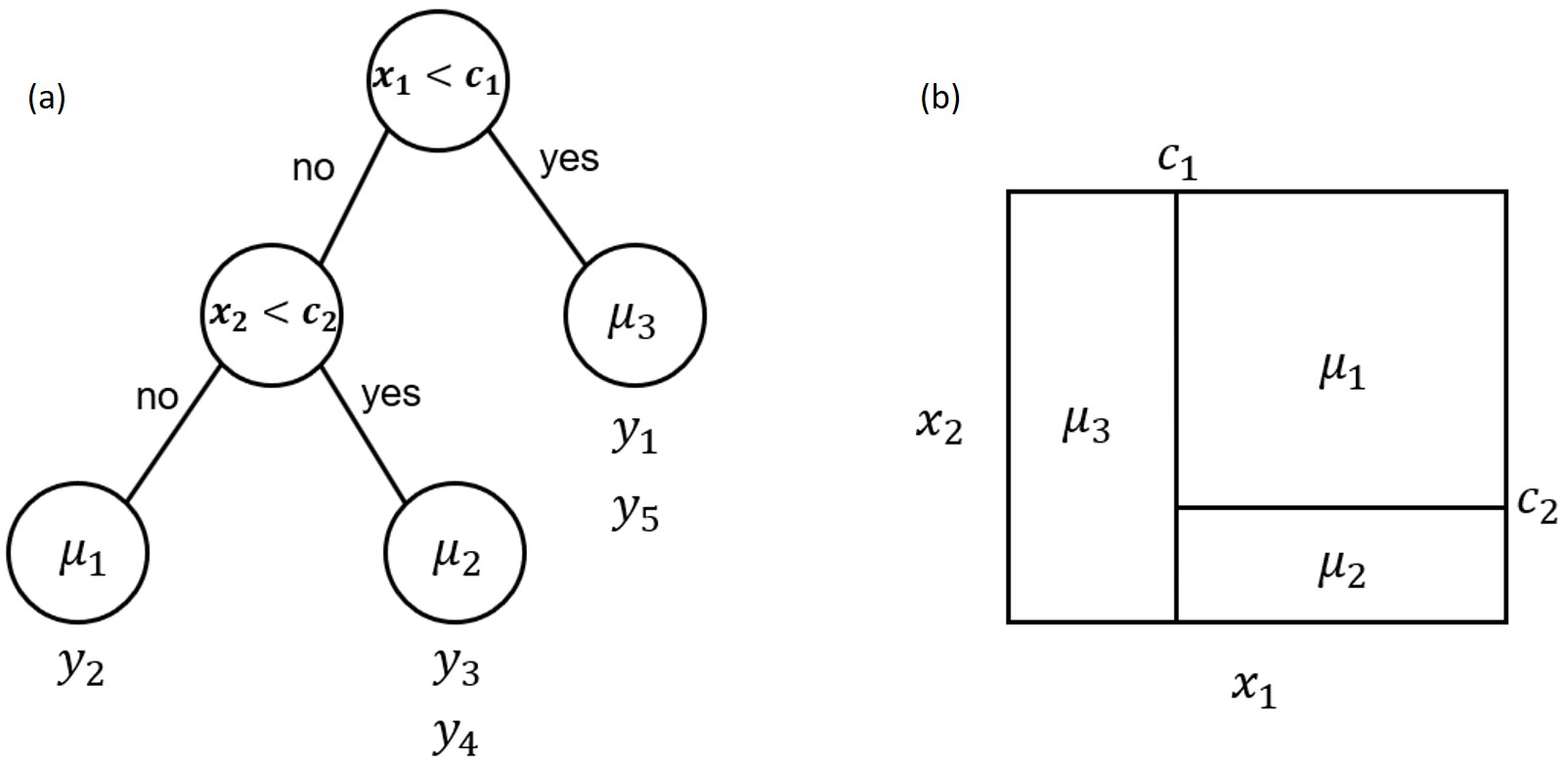
Figure 1: An example of binary regression tree model. (a) Tree structure includes the set of interior nodes with decision rules ($T$) and the set of parameter values associated with terminal nodes. (b) The step function $g(X,T,M)$ is depicted by the corresponding partition of the sample space.

In the original BART model (1) the errors are assumed to be $\epsilon_{i}\overset{\text{i.i.d}}{\sim}N(0,\sigma^{2})$. This assumption may not hold in general, for example, in modeling time series or spatial data. Therefore, we extend this assumption by allowing the errors to correlate with each other. Let $\Sigma$ denote a general covariance matrix, the correlated BART (CBART) can be defined as follows:

$$Y=\sum_{j=1}^{m}g(X;T_{j},M_{j})+\epsilon,\hskip 8.53581pt\epsilon\sim N(0,\Sigma),$$ (2)

where $Y=\{y_{1},\ldots,y_{n}\}$, $X=\{X_{1},\ldots,X_{n}\}$,$g(X;T_{j},M_{j})=\{g(X_{1};T_{j},M_{j}),\ldots,g(X_{n};T_{j},M_{j})\}$, and $\epsilon=\{\epsilon_{1},\ldots,\epsilon_{n}\}$.

2.1 Dummy representation

Similar to BART, the building block of CBART is the binary regression tree. In order to handle the covariance matrix, we propose a dummy representation (3) for the binary regression tree.

Definition 2.1 (Dummy representation).

$$g(X;T,M)=D\mu$$ (3)

where

$$D=\begin{bmatrix}d_{11}&d_{12}&...&d_{1b}\\ d_{21}&d_{22}&...&d_{2b}\\ \vdots&\vdots&\ddots\\ d_{n1}&d_{n2}&...&d_{nb}\end{bmatrix},\hskip 14.22636pt\mu=[\mu_{1},\mu_{2},...,\mu_{b}]^{T}.$$

In the matrix $D$, each row contains zeros in all entries except for the one linked to the bottom node to which the observation is mapped. For example, the $i^{th}$ row in $D$, $[d_{i1},...,d_{i,j-1},d_{i,j},d_{i,j+1},...,d_{in}]=[0,...,0,1,0,...0]$, demonstrates that the $i^{th}$ observation was mapped to the $j^{th}$ bottom node.

As an example, the dummy representation of the binary regression tree in Figure 1 is as follows. The matrix multiplication serves to map $\{y_{2}\}$ to $\mu_{1}$, $\{y_{3},y_{4}\}$ to $\mu_{2}$, and $\{y_{1},y_{5}\}$ to $\mu_{3}$. $$g(X;T,M)=D\mu=\begin{bmatrix}0&0&1\\ 1&0&0\\ 0&1&0\\ 0&1&0\\ 0&0&1\end{bmatrix}\begin{bmatrix}\mu_{1}\\ \mu_{2}\\ \mu_{3}\end{bmatrix}$$         
Based on the dummy representation, the individual regression tree model can be denoted as follows:

$$Y=g(X;T,M)+\epsilon=D\mu+\epsilon,\hskip 8.53581pt\epsilon\sim N(0,\Sigma).$$ (4)

2.2 Bayesian backfitting and Markov chain Monte Carlo

In order to fit the BART model in (1), Chipman et al. (2006, 2010) proposed a Bayesian backfitting (Hastie and Tibshirani, 2000) approach, using MCMC to update the pair $(T_{j},M_{j})$ conditioned on $\sigma$ and the remaining trees with their associated parameters. For the CBART, we need to replace $\sigma$ with $\Sigma$, then, the backfitting reparameterization can be presented as follows:

$$R_{j}=Y-\sum_{k\neq j}g(X;T_{k},M_{k})=g(X;T_{j},M_{j})+\epsilon,\hskip 8.53581pt\epsilon\sim N(0,\Sigma).$$ (5)

It is easy to check that (5) denotes an individual binary regression tree. As the subscript $j$ can take any value in $\{1,\ldots,m\}$, without loss of generality, we simplify the notation of (5) by omitting the subscript hereafter.

$$R=g(X;T,M)+\epsilon,\hskip 8.53581pt\epsilon\sim N(0,\Sigma).$$ (6)

In order to update $(T,M)|(R,\Sigma)$, by $p(T,M)=p(M|T)p(T)$, we need to update the follows:

$$T|R,\Sigma$$ (7)

$$M|T,R,\Sigma$$ (8)

(1) Updating $T$ through Metropolis-Hastings algorithmChipman et al. (1998) introduced the Metropolis–Hastings algorithm for updating $T$ in (7). This algorithm simulates a Markov chain which includes a sequence of states of the tree:

$$T^{0},T^{1},T^{2},\cdot\cdot\cdot$$

Starting from an initial state $T^{0}$, the state transition from $T^{i}$ to $T^{i+1}$, $i=0,1,2,...$, includes the following two steps:

• Given the current state $T^{i}$, generate a candidate state $T^{*}$ according to the transition kernel $q(T^{i},T^{*})$.

• Set $T^{i+1}=T^{*}$ with the probability,

  $$\alpha(T^{i+1}=T^{*})=min\{\frac{q(T^{*},T^{i})}{q(T^{i},T^{*})}\frac{p(R|X,T^{*})p(T^{*})}{p(R|X,T^{i})p(T^{i})},1\}.$$ (9)

  Otherwise, set $T^{i+1}=T^{i}$.

The terms $q(T^{*},T^{i}),q(T^{i},T^{*}),p(T^{*}),p(T^{i})$ in (9) are chosen in the same way as for BART. Therefore, the only part requiring consideration is the marginal likelihood ratio:

$$\frac{p(R|X,T^{*})}{p(R|X,T^{i})}=\frac{p(R|X,T^{i+1})}{p(R|X,T^{i})}.$$ (10)

Based on (4) and (6) with given $\Sigma$, we obtain

$$p(R|X,T)=p(R|D)=\int p(R|D,\mu)\pi(\mu)\,d\mu,$$ (11)

where

$$p(R|D,\mu)\sim N(D\mu,\Sigma),\hskip 8.53581pt\pi(\mu)\sim N(\bar{\mu},Q^{-1}),$$ (12)

mean $\bar{\mu}$ and precision matrix $Q$ are pre-specified hyperparameters.[Marginal distribution of $p(R|D)$]Given (11) and (12), the marginal distribution $p(R|D)$ can be expressed as follows:

$$p(R|D)=\frac{(2\pi)^{-\frac{n}{2}}|\Sigma|^{-\frac{1}{2}}|Q|^{\frac{1}{2}}}{|Q+D^{T}\Sigma^{-1}D|^{\frac{1}{2}}}exp\{-\frac{1}{2}(-v^{T}(Q+D^{T}\Sigma^{-1}D)v+\bar{\mu}^{T}Q\bar{\mu}+R^{T}\Sigma^{-1}R)\}$$ (13)

where, $v=(Q+D^{T}\Sigma^{-1}D)^{-1}(Q\bar{\mu}+D^{T}\Sigma^{-1}R)$.Since the mean is captured by other components of CBART (or as in BART the $y$ is demeaned) we can choose $\bar{\mu}=0$ so that (13) can be simplified to (14).

$$p(R|D)=\frac{(2\pi)^{-\frac{n}{2}}|\Sigma|^{-\frac{1}{2}}|Q|^{\frac{1}{2}}}{|Q+D^{T}\Sigma^{-1}D|^{\frac{1}{2}}}exp\{\frac{1}{2}[R^{T}\Sigma^{-1}D(Q+D^{T}\Sigma^{-1}D)^{-1}D^{T}\Sigma^{-1}R-R^{T}\Sigma^{-1}R]\}$$ (14)

Given (12), the product of likelihood and prior is as follows:

$$\begin{split}p(R|D,\mu)\pi(\mu)&=(2\pi)^{-\frac{n}{2}}|\Sigma|^{-\frac{1}{2}}exp\{-\frac{1}{2}(R-D\mu)^{T}\Sigma^{-1}(R-D\mu)\}*\\ &\hskip 15.0pt(2\pi)^{-\frac{b}{2}}|Q|^{\frac{1}{2}}exp\{-\frac{1}{2}(\mu-\bar{\mu})^{T}Q(\mu-\bar{\mu})\}\\ &=(2\pi)^{-\frac{n+b}{2}}|\Sigma|^{-\frac{1}{2}}|Q|^{\frac{1}{2}}*\\ &\hskip 15.0ptexp\{-\frac{1}{2}\underbrace{[(R-D\mu)^{T}\Sigma^{-1}(R-D\mu)+(\mu-\bar{\mu})^{T}Q(\mu-\bar{\mu})]}_{(*)}\}.\end{split}$$ (15)

where,

$$\begin{split}(*)&=R^{T}\Sigma^{-1}R-2R^{T}\Sigma^{-1}D\mu+\mu^{T}D^{T}\Sigma^{-1}D\mu+\mu^{T}Q\mu-2\bar{\mu}^{T}Q\mu+\bar{\mu}^{T}Q\bar{\mu}\\ &=\mu^{T}(D^{T}\Sigma^{-1}D+Q)\mu-2\underline{(R^{T}\Sigma^{-1}D+\bar{\mu}^{T}Q)}\mu+R^{T}\Sigma^{-1}R+\bar{\mu}^{T}Q\bar{\mu}.\end{split}$$

Let’s introduce a variable $v$ and consider the quadratic form:

$$\begin{split}&\hskip 15.0pt(\mu-v)^{T}(D^{T}\Sigma^{-1}D+Q)(\mu-v)\\ &=\mu^{T}(D^{T}\Sigma^{-1}D+Q)\mu-2\underline{v^{T}(D^{T}\Sigma^{-1}D+Q)}\mu+v^{T}(D^{T}\Sigma^{-1}D+Q)v.\end{split}$$

With the equivalence constraint of above underline coefficients,$v^{T}(D^{T}\Sigma^{-1}D+Q)=R^{T}\Sigma^{-1}D+\bar{\mu}^{T}Q$,we can obtain that

$$v=(Q+D^{T}\Sigma^{-1}D)^{-1}(Q\bar{\mu}+D^{T}\Sigma^{-1}R).$$ (16)

Therefore, $(*)=(\mu-v)^{T}(Q+D^{T}\Sigma^{-1}D)(\mu-v)+C$,where

$$C=-v^{T}(Q+D^{T}\Sigma^{-1}D)v+R^{T}\Sigma^{-1}R+\bar{\mu}^{T}Q\bar{\mu}.$$

Then, plug $(*)$ into (15):

$$\begin{split}&p(R|D)=\int p(R|D,\mu)p(\mu)d\mu\\ &=(2\pi)^{-\frac{n+b}{2}}|\Sigma|^{-\frac{1}{2}}|Q|^{\frac{1}{2}}exp\{-\frac{1}{2}C\}\int exp\{-\frac{1}{2}(\mu-v)^{T}(Q+D^{T}\Sigma^{-1}D)(\mu-v)\}d\mu\\ &=(2\pi)^{-\frac{n+b}{2}}|\Sigma|^{-\frac{1}{2}}|Q|^{\frac{1}{2}}exp\{-\frac{1}{2}C\}(2\pi)^{\frac{b}{2}}|Q+D^{T}\Sigma^{-1}D|^{-\frac{1}{2}}\\ &\hskip 35.0pt\cdot\int(2\pi)^{-\frac{b}{2}}|Q+D^{T}\Sigma^{-1}D|^{\frac{1}{2}}exp\{-\frac{1}{2}(\mu-v)^{T}(Q+D^{T}\Sigma^{-1}D)(\mu-v)\}d\mu\\ &=\frac{(2\pi)^{-\frac{n}{2}}|\Sigma|^{-\frac{1}{2}}|Q|^{\frac{1}{2}}}{|Q+D^{T}\Sigma^{-1}D|^{\frac{1}{2}}}exp\{-\frac{1}{2}C\}\end{split}$$

After simplification, we can get the expression in (13).

$$p(R|D)=\frac{(2\pi)^{-\frac{n}{2}}|\Sigma|^{-\frac{1}{2}}|Q|^{\frac{1}{2}}}{|Q+D^{T}\Sigma^{-1}D|^{\frac{1}{2}}}exp\{-\frac{1}{2}(-v^{T}(Q+D^{T}\Sigma^{-1}D)v+\bar{\mu}^{T}Q\bar{\mu}+R^{T}\Sigma^{-1}R)\},$$

where $v=(Q+D^{T}\Sigma^{-1}D)^{-1}(Q\bar{\mu}+D^{T}\Sigma^{-1}R)$.Based on Theorem 12, the marginal likelihood ratio in (10) is as follows:

$$\begin{split}&\frac{p(R|X,T^{i+1})}{p(R|X,T^{i})}=\frac{p(R|D^{i+1})}{p(R|D^{i})}=\frac{|Q^{i+1}|^{\frac{1}{2}}}{|Q^{i}|^{\frac{1}{2}}}\frac{|Q^{i}+(D^{i})^{T}\Sigma^{-1}D^{i}|^{\frac{1}{2}}}{|Q^{i+1}+(D^{i+1})^{T}\Sigma^{-1}D^{i+1}|^{\frac{1}{2}}}\cdot\\ &exp\{\frac{1}{2}R^{T}\Sigma^{-1}[D^{i+1}(Q^{i+1}+(D^{i+1})^{T}\Sigma^{-1}D^{i+1})^{-1}(D^{i+1})^{T}-\\ &D^{i}(Q^{i}+(D^{i})^{T}\Sigma^{-1}D^{i})^{-1}(D^{i})^{T}]\Sigma^{-1}R\}\end{split}$$ (17)

where the superscript $i$ and $i+1$ corresponds to state $i$ and state $i+1$, respectively.(2) Updating $M$ through the posterior distribution of $\mu$Based on the following Theorem 17, we can update $M$ in (8) by drawing $\mu$ from its posterior distribution.[Posterior distribution of $\mu$]

$$p(\mu|R)\sim N(\hskip 3.0pt(Q+D^{T}\Sigma^{-1}D)^{-1}(Q\bar{\mu}+D^{T}\Sigma^{-1}R)\hskip 3.0pt,\hskip 3.0pt(Q+D^{T}\Sigma^{-1}D)^{-1}\hskip 3.0pt)$$ (18)

Let $\bar{\mu}=0$, it can be simplified to

$$p(\mu|R)\sim N((Q+D^{T}\Sigma^{-1}D)^{-1}D^{T}\Sigma^{-1}R,(Q+D^{T}\Sigma^{-1}D)^{-1}).$$ (19)

Given $D$ and $\Sigma$, the posterior distribution of $\mu$ is proportional to the product of its likelihood and prior as follows:

$$p(\mu|R)\propto p(R|\mu)\pi(\mu)=p(R|D,\mu)\pi(\mu),$$ (20)

where $p(R|D,\mu)\sim N(D\mu,\Sigma)$ and $\pi(\mu)\sim N(\bar{\mu},Q^{-1})$.Then, conduct the same derivation in (15) and (16), we can prove that

$$p(\mu|R)\sim N(\hskip 3.0pt(Q+D^{T}\Sigma^{-1}D)^{-1}(Q\bar{\mu}+D^{T}\Sigma^{-1}R)\hskip 3.0pt,\hskip 3.0pt(Q+D^{T}\Sigma^{-1}D)^{-1}\hskip 3.0pt).$$ (21)

2.3 Efficient matrix computation

As discussed in Section 2.2, it is evident that the primary computational burden in CBART arises from (17) and (19), both of which are dominated by matrix operations. For a deeper understanding of the computation complexity, let’s set

$$A=Q+D^{T}\Sigma^{-1}D.$$ (22)

It is a $b\times b$ symmetric matrix, with $b$ representing the number of bottom nodes in the individual tree. In (17) and (19), we need to compute $|A|$ and $A^{-1}$, both requiring $O(b^{3})$ operations. As CBART (similarly to BART) penalizes tree size, i.e., the number of bottom nodes, $b$ is typically small (less than 20). Therefore, given $A$, the computation for CBART is not challenging. However, the challenge lies in calculating the matrix $A$. For the computation in (22), $\Sigma^{-1}$ demands $O(n^{3})$ operations, where $n$ is the number of observations. Fortunately, in applications such as time series and spatial data analysis, the matrix $\Sigma^{-1}$ can be well approximated with only $O(n)$ operations. These approximation methods have been extensively studied in both applied mathematics (Hackbusch, 2015; Lin et al., 2011) and statistics (Datta et al., 2016; Finley et al., 2019; Litvinenko et al., 2019). Therefore, in such situations, each iteration of MCMC requires $O(n)$ operations.The special structure of the matrix $D$ in dummy representation offers an opportunity to improve the efficiency of the computations in MCMC updating. To take advantage of the dummy representation, we need to reorder the matrix $D$ to a particular form. We illustrate the reordering process using the example in Figure 1, as follows:

$$D=\begin{bmatrix}0&0&1\\ 1&0&0\\ 0&1&0\\ 0&1&0\\ 0&0&1\end{bmatrix}=PD_{P}=\begin{bmatrix}0&0&0&0&1\\ 1&0&0&0&0\\ 0&1&0&0&0\\ 0&0&1&0&0\\ 0&0&0&1&0\end{bmatrix}\begin{bmatrix}1&0&0\\ 0&1&0\\ 0&1&0\\ 0&0&1\\ 0&0&1\end{bmatrix}$$

The matrix $D$ is reordered to $D_{P}$ using the permutation matrix $P$. Subsequently, the well-organized $D_{P}$ can collaborate with the matrix blocking technique to achieve computational efficiency.

Definition 2.2 (Reordering).

The matrix $D$ in dummy representation (3) can be reordered to $D_{P}$ using a permutation matrix $P$, as follows:

$$D=PD_{P},\hskip 8.53581ptP^{T}D=D_{P},$$ (23)

where

$$D_{P}=\begin{bmatrix}d^{\prime}_{11}&d^{\prime}_{12}&...&d^{\prime}_{1b}\\ d^{\prime}_{21}&d^{\prime}_{22}&...&d^{\prime}_{2b}\\ \vdots&\vdots&\ddots\\ d^{\prime}_{n1}&d^{\prime}_{n2}&...&d^{\prime}_{nb}\end{bmatrix},\hskip 8.53581ptd^{\prime}_{ij}=\begin{cases}0,&i\notin\Omega_{j},\\ 1,&i\in\Omega_{j}.\end{cases}\hskip 15.0pti=1,...,n;\hskip 15.0ptj=1,...,b,$$

$\Omega_{j}$ is the index set of observations that be mapped to $j^{th}$ bottom node.

For consistency, it is imperative to simultaneously reorder $\{D,R,\Sigma\}$ to $\{D_{P},R_{P},\Sigma_{P}\}$ using the same permutation matrix $P$, as follows:

$$D=PD_{P},\hskip 8.53581ptR=PR_{P},\hskip 8.53581pt\Sigma=P\Sigma P^{T}.$$ (24)

[Reordering invariance]Reordering does not change the value of the marginal likelihood ratio in (17).

$$\begin{split}\frac{p(R|D^{i+1})}{p(R|D^{i})}=&\frac{|Q^{i+1}|^{1/2}}{|Q^{i}|^{1/2}}\frac{|Q^{i}+(D_{P}^{i})^{T}\Sigma_{P}^{-1}D_{P}^{i}|^{1/2}}{|Q^{i+1}+(D_{P}^{i+1})^{T}\Sigma_{P}^{-1}D_{P}^{i+1}|^{1/2}}\cdot\\ &exp\{\frac{1}{2}R_{P}^{T}\Sigma_{P}^{-1}[D_{P}^{i+1}(Q^{i+1}+(D_{P}^{i+1})^{T}\Sigma_{P}^{-1}D_{P}^{i+1})^{-1}(D_{P}^{i+1})^{T}\\ &-D_{P}^{i}(Q^{i}+(D_{P}^{i})^{T}\Sigma_{P}^{-1}D_{P}^{i})^{-1}(D_{P}^{i})^{T}]\Sigma_{P}^{-1}R_{P}\}\end{split}$$ (25)

Since $P$ is a permutation matrix, it has the property $P^{-1}=P^{T}$. With (23) and (24), we can obtain the following:

$$\begin{split}D^{T}\Sigma^{-1}R&=(PD_{P})^{T}(P\Sigma_{P}P^{T})^{-1}(PR_{P})\\ &=D_{P}^{T}P^{T}P\Sigma_{P}^{-1}P^{T}PR_{P}\\ &=D_{P}^{T}\Sigma_{P}^{-1}R_{P}\\ \end{split}$$ (26)

Given $Q=\tau^{-2}I$, we can get

$$Q+D^{T}\Sigma^{-1}D=Q+(PD_{P})^{T}P\Sigma_{P}^{-1}P^{T}PD_{P}=Q+D_{P}^{T}\Sigma_{P}^{-1}D_{P}.$$ (27)

Plug (24), (26), (27) into (17), we can prove the theorem is hold.

$$\begin{split}\frac{p(R|D^{i+1})}{p(R|D^{i})}&=\frac{|Q^{i+1}|^{\frac{1}{2}}}{|Q^{i}|^{\frac{1}{2}}}\frac{|Q^{i}+(D^{i})^{T}\Sigma^{-1}D^{i}|^{\frac{1}{2}}}{|Q^{i+1}+(D^{i+1})^{T}\Sigma^{-1}D^{i+1}|^{\frac{1}{2}}}\cdot exp\{\frac{1}{2}R^{T}\Sigma^{-1}[D^{i+1}(Q^{i+1}+\\ &(D^{i+1})^{T}\Sigma^{-1}D^{i+1})^{-1}(D^{i+1})^{T}-D^{i}(Q^{i}+(D^{i})^{T}\Sigma^{-1}D^{i})^{-1}(D^{i})^{T}]\Sigma^{-1}R\}\\ &=\frac{|Q^{i+1}|^{1/2}}{|Q^{i}|^{1/2}}\frac{|Q^{i}+(D_{P}^{i})^{T}\Sigma_{P}^{-1}D_{P}^{i}|^{1/2}}{|Q^{i+1}+(D_{P}^{i+1})^{T}\Sigma_{P}^{-1}D_{P}^{i+1}|^{1/2}}\cdot exp\{\frac{1}{2}R_{P}^{T}\Sigma_{P}^{-1}[D_{P}^{i+1}(Q^{i+1}+\\ &(D_{P}^{i+1})^{T}\Sigma_{P}^{-1}D_{P}^{i+1})^{-1}(D_{P}^{i+1})^{T}-D_{P}^{i}(Q^{i}+(D_{P}^{i})^{T}\Sigma_{P}^{-1}D_{P}^{i})^{-1}(D_{P}^{i})^{T}]\Sigma_{P}^{-1}R_{P}\}\end{split}$$

The update for $T$ in (7) involves two node operations: birth and death. Birth entails the creation of two child nodes from a leaf node, while death involves removing the two sibling leaf nodes from their parent. For both operations, we need to calculate the marginal likelihood ratio, which is computationally intensive. Based on Theorem 24, we introduce an efficient approach in Appendix B to calculate the marginal likelihood ratio in (25) by leveraging the technique of matrix blocking.

2.4 Example: comparison of CBART and BART

To illustrate the similarities and differences between CBART and BART, let’s introduce an example with data generated from the following model:

$$y_{i}=f(x_{i})+\eta_{i},\hskip 14.22636pti\in\{1,...,n\},$$ (28)

where $n=200$, $f(x_{i})=x_{i}^{3}$, $x_{i}$ generated from a uniform distribution in $(-1,1)$, $\boldsymbol{\eta}=\{\eta_{1},...,\eta_{n}\}$ and $\boldsymbol{\eta}\sim N(0,\Sigma)$.We consider two different dependent structures of $\eta$.

• $\eta_{i}$ are independent and identically distributed (i.i.d.).In this case, $\Sigma=\sigma^{2}I$, and CBART should be identical to BART.

• $\eta_{i}$ are correlated.In this case, $\eta_{i}$ was generated as follows:

  $$\eta_{i}=\rho\epsilon_{i-1}+\epsilon_{i},\hskip 8.53581pt0<\rho<1,\hskip 8.53581pt\epsilon_{0}=0,\hskip 8.53581pt\epsilon_{i}\sim N(0,\sigma^{2}),\hskip 8.53581pti=1,...,n.$$

  We can denote $\boldsymbol{\eta}$ in a matrix form, $\boldsymbol{\eta}=A\boldsymbol{\epsilon}$, where

  $$\boldsymbol{\eta}=\begin{bmatrix}\eta_{1}\\ \vdots\\ \eta_{n}\end{bmatrix},\hskip 15.0ptA=\begin{bmatrix}1&0&0&\ldots&0&0\\ \rho&1&0&\ldots&0&0\\ 0&\rho&1&\ldots&0&0\\ \vdots&\vdots&\ddots&\ddots&\vdots&\vdots\\ 0&0&0&\ldots&\rho&1\end{bmatrix}_{n\times n},\hskip 15.0pt\boldsymbol{\epsilon}=\begin{bmatrix}\epsilon_{1}\\ \vdots\\ \epsilon_{n}\end{bmatrix}.$$ (29)

  Thus, $\Sigma=\sigma^{2}AA^{T}$ and $\Sigma^{-1}=\sigma^{-2}A^{-T}A^{-1}$.

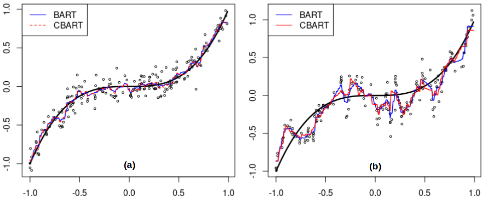
Figure 2: Panel (a) illustrates the consistency of CBART and BART when the errors are i.i.d. Panel (b) highlights the distinction between CBART and BART in the presence of correlated errors. Further details on the comparison can be found in Table 1.

Our goal is to estimate the regression function $E[y|x]=f(x)$. Figure 2 presents the fitted BART and CBART. In panel (a) showing the i.i.d. case, CBART is consistent with BART. In panel (b) depicting the correlated case, where $\Sigma$ is given with the true values of $\sigma=0.1$ and $\rho=0.8$, CBART obviously differs from BART. To gain a deeper understanding of these differences, we compare BART and CBART using two criteria: their performance in terms of fitting to the data (fitting-to-data) or fitting to the true function $f(x)$ (fitting-to-$f(x)$). On one hand, under the criterion of fitting-to-data, CBART performed worse than BART, with a 53.6% increase in MSE and a 3.5% decrease in $R^{2}$. On the other hand, under the criterion of fitting-to-$f(x)$, CBART outperformed BART, showing a 15.7% reduction in MSE. This indicates that CBART has the capability to improve the estimation of the underlying true regression function when the dependent structure of the data is well estimated.

Table 1: Two comparison criteria: fitting-to-data versus fitting-to-$f(x)$.

Model	Fitting-to-data		Fitting-to-$f(x)$
	$R^{2}$	MSE	MSE
$BART$	93.9%	0.0086	0.0184
$CBART$	90.6%	0.0132	0.0155
$\dfrac{CBART-BART}{BART}$	-3.5%	53.6%	-15.7%

3 Gaussian processes CBART

In spatial statistics, linear mixed regression models (LMX) in (30) are widely applied and well-studied (Goldberger, 1962; Pebesma, 2006; Cressie, 2015).

$$y(s_{i})=X(s_{i})\beta+w(s_{i})+\epsilon(s_{i}),\hskip 8.53581pt\epsilon(s_{i})\overset{\text{i.i.d.}}{\sim}N(0,\tau^{2})$$ (30)

• $s_{i}$: a spatial position, $i=1,2,...,n$;

• $y(s_{i})$: the response at $s_{i}$;

• $X(s_{i})$: the covariates at $s_{i}$;

• $\beta$: the coefficients of covariates;

• $w(s_{i})$: a stationary Gaussian processes with zero mean;

• $\epsilon(s_{i})$: the pure error at $s_{i}$.

One of the advantages of LMX is its capability to model the dependent structure in the response through the Gaussian processes, $w(s_{i})$, which can account for the influence of unobserved covariates. However, the assumption of the linear regression function, $X(s_{i})\beta$, may not always hold in practice. To address this, and substituting it with CBART, we propose a novel nonlinear mixed regression model as follows:

$$y(s_{i})=f_{CBART}(X(s_{i}))+w(s_{i})+\epsilon(s_{i})$$ (31)

The CBART regressor, $f_{CBART}(X(s_{i}))$, will capture the nonlinear relationship between covariates and response. We designate this model in (31) as GP-CBART.

3.1 Identification and degeneration issues in full Bayesian approach

Gibbs sampling appears to be a promising full Bayesian solution for GP-CBART in (31), as follows:

$$\Sigma(\boldsymbol{\theta})\ |\ f_{CBART}$$ (32)

$$f_{CBART}\ |\ \Sigma(\boldsymbol{\theta})$$ (33)

where $\boldsymbol{\theta}$ denotes all parameters in $w(s)$ and $\epsilon(s)$.Regarding (32), given $f_{CBART}$, we can represent the full Bayesian expression of (31) as follows:

$$p(\boldsymbol{\theta}|y)\propto N(y|f_{CBART}+w(s),\tau^{2}\boldsymbol{I})\times N(w(s)|0,\boldsymbol{C})\times p(\boldsymbol{\theta})$$ (34)

where $\boldsymbol{C}$ is a covariance matrix generated by a kernel function $C(s_{i},s_{j})$.Leveraging the norm property of Gaussian processes $w(s)$, we can integrate it out to obtain:

$$p(\boldsymbol{\theta}|y)\propto N(y|f_{CBART},\boldsymbol{C}+\tau^{2}\boldsymbol{I})\times p(\boldsymbol{\theta}).$$

Obviously, $\Sigma(\boldsymbol{\theta})=\boldsymbol{C}+\tau^{2}\boldsymbol{I}$, and, the posterior $p(\boldsymbol{\theta}|y)$ can be presented as follows:

$$p(\boldsymbol{\theta}|y)\propto\frac{1}{\sqrt{|\Sigma(\boldsymbol{\theta})|}}exp\{-\frac{1}{2}(y-f_{CBART})^{T}\Sigma^{-1}(\boldsymbol{\theta})(y-f_{CBART})\}\times p(\boldsymbol{\theta})$$ (35)

By using (35), we can update (32). The update of (33) has been thoroughly discussed in Section 2. Although the Gibbs sampling strategy looks good so far, two issues impede its success. To illustrate these issues, let’s consider an example in which the data is generated as follows:

$$f(x(s_{i}))=x(s_{i})^{3},\hskip 15.0ptx(s_{i})\sim unif(1,3),\hskip 15.0pti=1,...,n,$$

$$w(s)\sim GP(0,C(\cdot)),\hskip 8.53581ptC(|s_{i}-s_{j}|)=\sigma^{2}exp\{-|s_{i}-s_{j}|/\phi\},\hskip 8.53581pt\epsilon(s_{i})\overset{\text{i.i.d.}}{\sim}N(0,\tau^{2}),$$

where $\sigma=1$, $\tau=1$, $\phi=6$, and $unif(1,3)$ denotes uniform distribution in $(1,3)$.

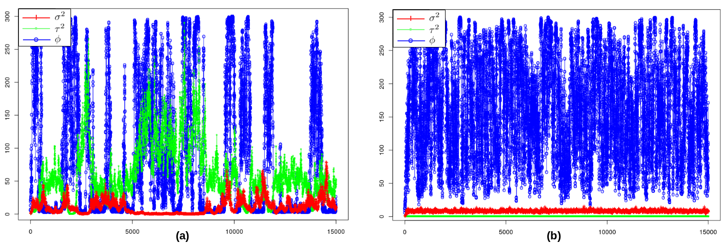
Figure 3: Identification and degeneration issues. (a) identification issue: the Markov chains cannot achieve stationary. (b) degeneration issue: CBART degenerates to BART.

The MCMC chains of parameters, $\tau^{2}$, $\sigma^{2}$, and $\phi$, are shown in Figure 3. In panel (a), the chains fail to achieve stationarity. This issue may arise because both CBART and the Gaussian processes are highly flexible and sensitive to changes in other parameters during the MCMC process. Small perturbations may result in dramatic turbulence, preventing the posterior from reaching stationarity. Consequently, the parameters cannot be properly identified, and we refer to this problem as the identification issue.In an attempt to address this issue, we set the parameter $\tau$ to its true value, i.e., $\tau=1$. In this case, the chains for $\sigma^{2}$ and $\phi$ achieved stationarity, as shown in Figure 3 (b). However, the estimate of $\phi$ is excessively large (approximately $150$), resulting in the covariance matrix $\Sigma=\tau^{2}I$, as follows:

$$C(|s_{i}-s_{j}|)=\sigma^{2}exp\{-\phi|s_{i}-s_{j}|\}\approx\sigma^{2}exp\{-150\cdot|s_{i}-s_{j}|\}\approx 0,$$

$$\Sigma=\boldsymbol{C}+\tau^{2}\boldsymbol{I}\approx\boldsymbol{0}+\tau^{2}\boldsymbol{I}=\tau^{2}\boldsymbol{I}.$$

In this case, CBART degenerates to BART, and we refer to this problem as the degeneration issue. Let’s revisit the example in Section 2.4 to identify a potential explanation for this issue. In Table 1, CBART exhibits poorer performance than BART in fitting the data, even with the true values of the parameters ($\rho$ and $\sigma$). In fact, CBART’s performance worsens as $|\rho|$ approaches 1 (with fixed $\sigma$). This suggests that the advantage of capturing the correlation structure comes at the expense of a suboptimal data fit, translating to a low likelihood. This outcome is unexpected, as MCMC typically seeks parameter values in the parameter space based on high likelihood criteria. Consequently, the MCMC algorithm tends to prioritize achieving a good data fit over capturing the correlation structure. As a result, the matrix $\boldsymbol{C}$ tends to approach 0, causing CBART to degenerate into BART.In conclusion, the full Bayesian approach proposed in (32) and (33) does not work for GP-CBART due to the identification and degradation issues.

3.2 Analysis of variation

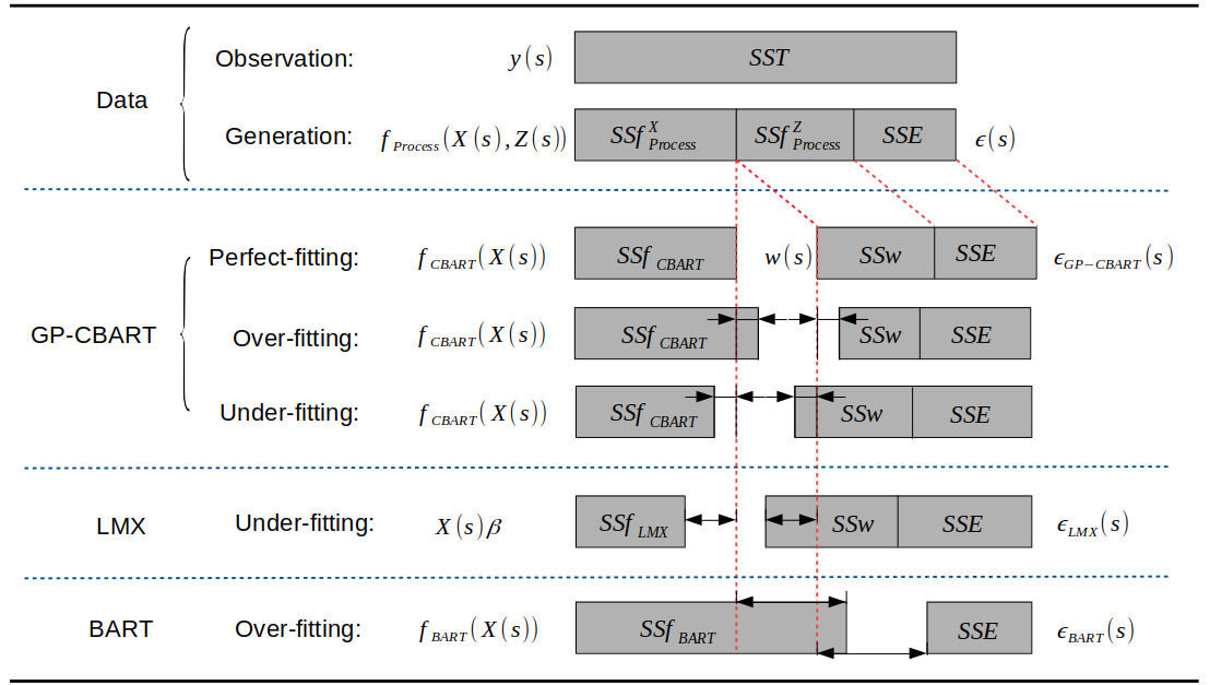
Figure 4: Analysis of variation.

To address the identification and degradation issues, a deeper understanding of GP-CBART is essential. Figure 4 offers insights from the perspective of variation decomposition. We assume that observations are generated by an underlying data-generating process, $f_{Process}(X(s),Z(s))$, where $X(s)$ and $Z(s)$ denote observed and unobserved covariates, respectively. The total variation of the observations is divided into three parts: $SSf^{X}_{process}$, $SSf^{Z}_{process}$, and $SSE$, representing the variation explained by $X(s)$, $Z(s)$, and pure errors $\epsilon(s)$. In GP-CBART, the counterparts are $f_{CBART}(X(s))$, $w(s)$, and $\epsilon(s)$, respectively. The linear mixed model (LMX) tends to underestimate $f_{Process}(X(s))$ compared to GP-CBART when $f_{Process}(X(s))$ is nonlinear. In contrast, the BART model tends to overestimate $f_{Process}(X(s))$ as $f_{BART}(X(s))$ likely includes the effects of both $X(s)$ and $Z(s)$. As Figure 4 shows, although GP-CBART may possibly under- or overestimate $f_{BART}(X(s))$, it has the potential for achieving a good fit.

3.3 Back comparing and tuning range

Based on the idea of variation decomposition, we propose an approach to intervene in the parameter search process to find optimal parameter values, as illustrated in Figure 5. Initially, we define a set of parameter values, denoted as $\mathcal{S}=\{\boldsymbol{\theta^{(0)}},\ldots,\boldsymbol{\theta^{(n)}}\}$, within which we search for promising candidates. Subsequently, for each $\boldsymbol{\theta^{(i)}}$ in $\mathcal{S}$, we calculate the proposed mean squared error of GP and pure noise, $MSE_{proposed}$, attributed to $w(s)+\epsilon(s)$ with $\boldsymbol{\theta^{(i)}}$. Conversely, utilizing the same $\boldsymbol{\theta^{(i)}}$, we fit the CBART model and compute $MSE_{real}=\sum_{i=1}^{n}[y(s_{i})-f_{CBART}(X(s_{i}))]^{2}/n$, representing the actual mean squared error not explained by CBART. In this context, three possible scenarios arise in the comparison of $MSE_{proposed}$ and $MSE_{real}$ as follows:

• $MSE_{proposed}<MSE_{real}$ : under-estimation, $MSE_{real}$ is under-estimated by $MSE_{proposed}$.

• $MSE_{proposed}>MSE_{real}$ : over-estimation, $MSE_{real}$ is over-estimated by $MSE_{proposed}$.

• $MSE_{proposed}\approx MSE_{real}$ : good-estimation, $MSE_{real}$ is well estimated by $MSE_{proposed}$.

We name this comparison process “back comparing”. Subsequently, the proposed candidate $\boldsymbol{\theta^{(i)}}$ associated with the good-estimation is recognized as a good candidate, and the set of good candidates, $\mathcal{T}$, is referred to as the “tuning range”.

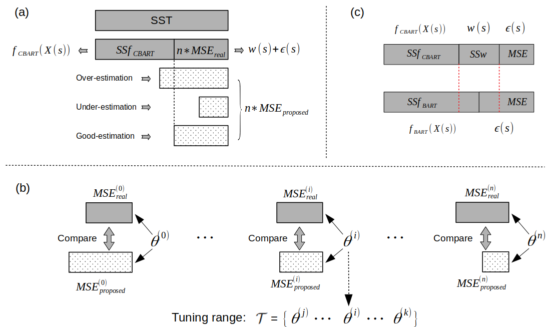
Figure 5: (a) Back comparing for identifying the good estimation. (b) Tuning range including the good candidates. (c) Variation decomposition for understanding suitable parameter value selection in the tuning range.

Technically, the GP-CBART model with any parameter value in the tuning range fits well with the data. The researcher can choose the one most suitable for their application. Based on the idea of variation decomposition, panel (c) in Figure 5 provides clues for selecting the suitable parameter value from the tuning range. The difference between GP-CBART and BART lies in the component $w(s)$. When we choose a parameter value that results in a notable variation explained by $w(s)$, where $SSw$ is comparable to $SSf_{CBART}$ and $SSE$, it indicates that the variation explained by the observed covariates through CBART is relatively small. In this case, CBART tends not to overfit the data compared to BART, as illustrated in the example in Figure 2. Therefore, selecting a parameter value to amplify the effects of $w(s)$ can enhance the robustness of CBART. On the other hand, since $w(s)$ is used to capture the effects of unobserved covariates in GP-CABRT, if there are any missing covariates (factors) in the application, a smart strategy is to increase the effects of $w(s)$ by selecting the parameter that maximizes the variation explained by $w(s)$. More details about the back comparing and tuning range can be found in Section 4.1.

4 Simulation Studies

In this section, we conduct two simulation studies with one-dimensional and two-dimensional data, respectively. These studies illustrate the advantages of GP-CBART from the perspective of variation decomposition and provide details on the approaches of back comparing and tuning range.

4.1 One-dimensional study

We use the same dataset as in the example (28) in Section 2.4. To simplify the discussion, we employ the just-right GP-CBART model as follows:

$$y_{i}=f_{CBART}(x_{i})+\eta_{i}$$ (36)

where

$$\eta_{i}=\rho\epsilon_{i-1}+\epsilon_{i},\hskip 8.53581pt\epsilon_{0}=0,\hskip 8.53581pt\epsilon_{i}\sim N(0,\sigma^{2}),\hskip 8.53581pti=1,..,n.$$

Same to (28), $\boldsymbol{\eta}$ denote the sequence $\{\eta_{i}\}$. Form (29), we know $\boldsymbol{\eta}\sim N(0,\Sigma)$, where $\Sigma=\sigma^{2}AA^{T}$. Therefore, $\eta_{i}$ is a Gaussian process. The parameters of model (36) are $\boldsymbol{\theta}=\{\sigma,\rho\}$.Their true values are $\sigma=0.1$ and $\rho=0.8$, respectively. In contrast to the example (28) in Section 2.4, we do not know these true values and need to estimate them using the approaches of back comparing and tuning range.

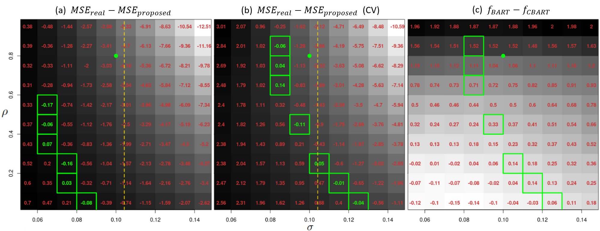
Figure 6: Back comparing and tuning range. The green dot in each panel denotes the true parameter value. The vertical yellow dashed line represents the estimate $\sigma$ from BART. The green cells correspond to the candidates in tuning range. Panel (a) shows the tuning range that was identified by the whole data (used to fit the model). While, the tuning range in panel (b) was estimated through 4-folds cross-validation. Panel (c) is used for guiding the selection of best parameter value in the tuning range.

As discussed in Section 3.3, applying back comparing involves specifying the set $\mathcal{S}=\{\boldsymbol{\theta^{(1)}},...,\boldsymbol{\theta^{(n)}}\}$, where the true values may be located. A clue for the true value of $\sigma$ can be provided by the BART estimation, $\hat{\sigma}_{BART}=0.1042189$, which is marked by the yellow dashed line in Figure 6 (a) and (b). We can search $\sigma$ in the neighbor interval of $\hat{\sigma}_{BART}$, in the interval $(0.05,0.15)$. For the parameter $\rho$, its value must fall in $(0,1)$ to keep the stationary of the Gaussian process. We divided each of the two intervals into 10 segments and selected their center as the possible values of parameters. The set $\mathcal{S}=\{\boldsymbol{\theta^{(1)}},...,\boldsymbol{\theta^{(100)}}\}$ is shown in Figure 6.In the second step, we need to compare $MSE_{real}$ and $MSE_{proposed}$ to identify the tuning range, including the good-estimation candidates. Figure 6 (a) and (b) show the results of $MSE_{real}-MSE_{proposed}$. The grids with negative/positive values represent over-estimation/under-estimation. The tuning range, which is the set of green grids, is selected under a strict criterion $|MSE_{real}-MSE_{proposed}|<0.2$. Panel (a) shows the results obtained by working on the entire dataset. However, in this case, CBART tends to overfit the data and causes the parameters to be underestimated. To address this issue, we use a 4-folds cross-validation to estimate the predictive values of $MSE_{real}-MSE_{proposed}$, as presented in panel (b). The number of folds in cross-validation should not be too large to avoid harming the estimation of the correlation parameter $\rho$. A large number of folds produce a small testing dataset, which then leads to a remarkable change in the dependency structure.

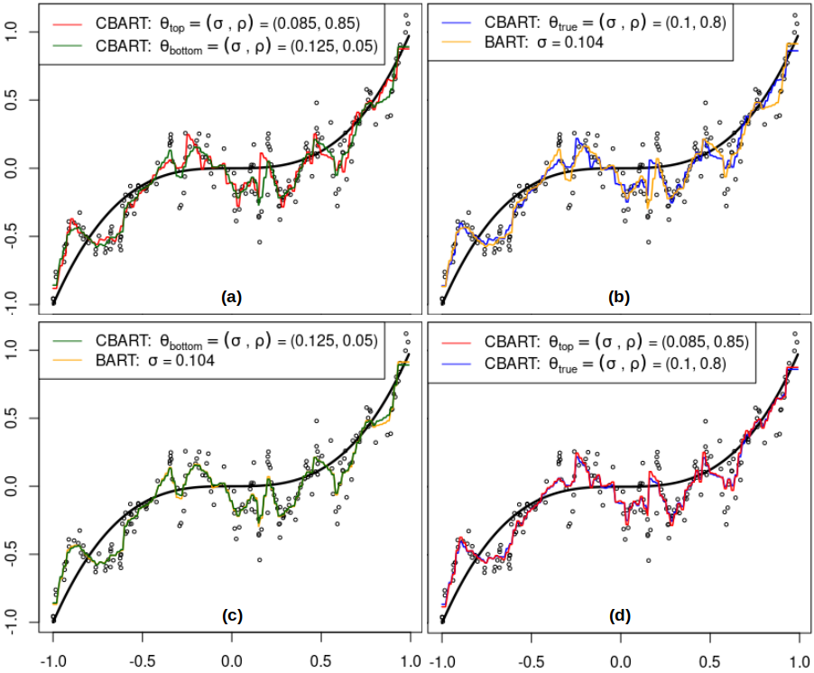
Figure 7: Understanding the tuning range. (a) The two extreme candidates in the tuning range. (b) CBART with the true parameters and the BART. (c) The bottom candidate in the tuning range corresponds to the BART. (d) The top candidate in the tuning range corresponds to the CBART with true parameters.

Our goal is to estimate the regression function $E[y|x]=f(x)$. The panel (c) in Figure 6 shows the estimated value of $SSf_{BART}-SSf_{CBART}$. As discussed in Section 3.3, the larger this value, the more robust the CBART is. Therefore, under the robust criterion, the top green grid with the value 1.52 corresponds to the optimal candidate, $\boldsymbol{\theta}_{\text{top}}=\{\sigma,\rho\}=\{0.085,0.85\}$, which is also close to the true values $\{0.1,0.8\}$. Compared to $f_{BART}(x)$, the $f_{CBART}(x)$ fitted under these parameter values is a more accurate estimate of the regression function $E[y|x]=f(x)$. The MSE fitting to the true $f(x)$ are 0.0184 and 0.0172 for BART and CBART, respectively. The percentage reduction in MSE for $f_{CBART}(x)$ is 6.4% compared to $f_{BART}(x)$.For a deeper understanding of the tuning range, let’s consider two extreme candidates in the tuning range, $\boldsymbol{\theta}_{\text{top}}=\{\sigma,\rho\}=\{0.085,0.85\}$ and $\boldsymbol{\theta}_{\text{bottom}}=\{\sigma,\rho\}=\{0.125,0.05\}$. Figure 7 presents the comparison between these extreme candidates versus the true values $\boldsymbol{\theta}_{\text{true}}=\{\sigma,\rho\}=\{0.1,0.8\}$ and the BART model. For the fitted $f_{CBART}(x)$, the one with $\boldsymbol{\theta}_{\text{top}}$ is close to the one with $\boldsymbol{\theta}_{\text{true}}$, while the one with $\boldsymbol{\theta}_{\text{bottom}}$ is close to the $f_{BART}(x)$. These observations indicate that we can tune CBART’s degree of fitting-to-data by selecting different parameter values in the tuning range. The highest degree corresponds to the case where CBART degenerates to BART, while the lowest degree corresponds to the case where the dependency in the data plays a significant role. We need to choose the one within the tuning range that best fits our application.

4.2 Two-dimensional study

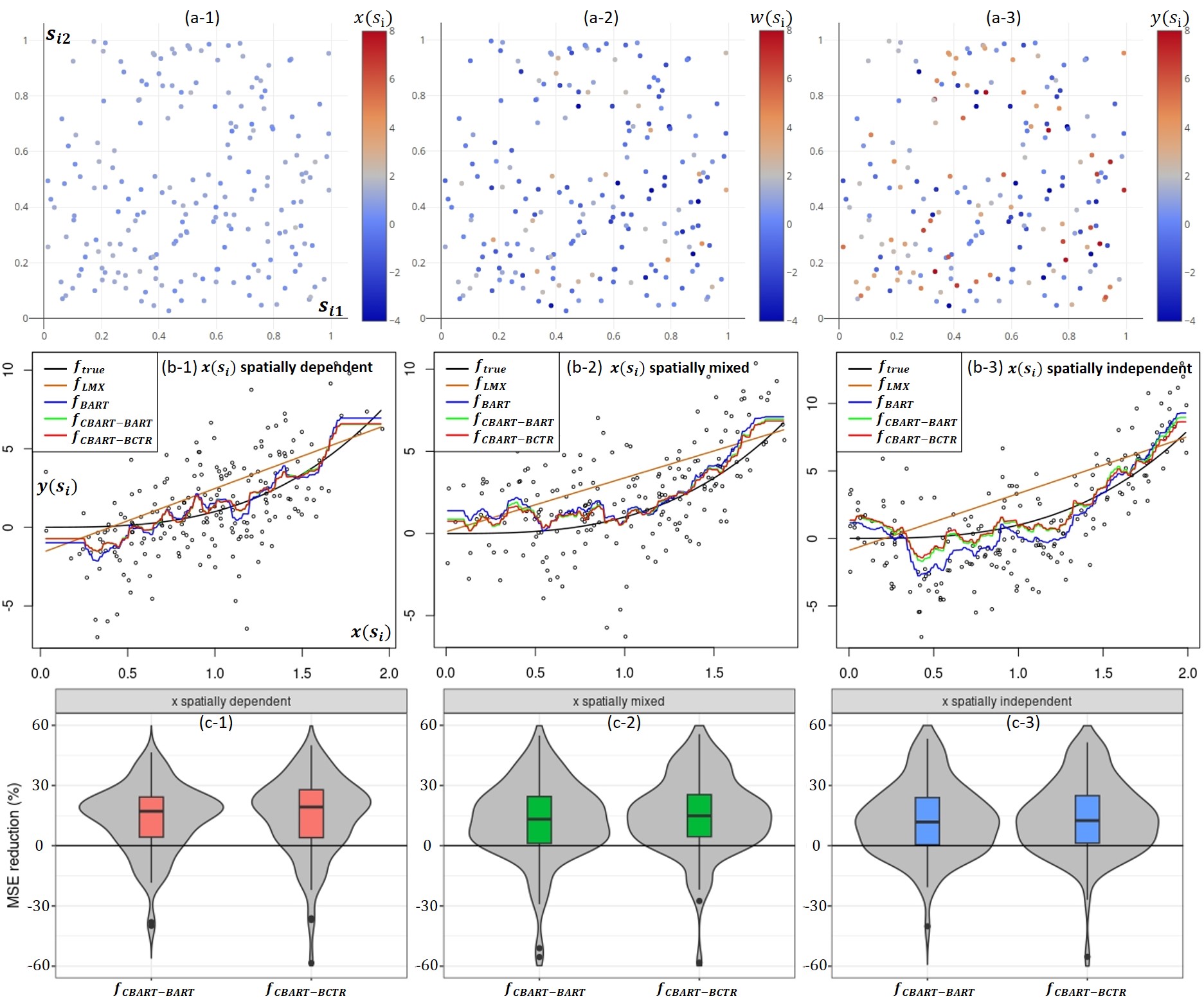
Figure 8: Two-dimensional simulation study results. (a-1,2,3) An example of the simulated two-dimensional data. (b-1,2,3) Examples of different $x(s_{i})$ and the comparison of fitted models, $f_{LMX}$, $f_{BART}$, $f_{CBART-BART}$, and $f_{CBART-BCTR}$. (c-1,2,3) The MSE reduction of $f_{CBART-BART}$ and $f_{CBART-BCTR}$ compared to $f_{BART}$ under the criterion of fitting-to-$f(x)$. This 100 simulations result demonstrates the superiority of GP-CBART compared to BART in estimating the true regression function.

Section 4.1 details the process of back comparing and tuning range, demonstrating its effectiveness. However, this approach encounters challenges in both identifying $\mathcal{S}=\{\boldsymbol{\theta}^{(1)},...,\boldsymbol{\theta}^{(n)}\}$ and maintaining computational efficiency as the number of parameters increases. For instance, in spatial regression models, the Matérn covariance functions are commonly employed. The component $w(s_{i})+\epsilon(s_{i})$ involves three parameters for estimation, ${\sigma,\phi,\tau}$. In such cases, identifying the set $\mathcal{S}$ in a three-dimensional space becomes challenging, requiring consideration of a substantial number of candidates in $\mathcal{S}$, thereby exacerbating the computational burden. In this section, we introduce two efficient methods to address these challenges.The simulation focuses on spatial data analysis, where the model and parameters employed for generating simulation data are as follows.

$$y(s_{i})=f(x(s_{i}))+w(s_{i})+\epsilon(s_{i}),\hskip 14.22636pti\in\{1,...,200\}$$

• $s_{i}=(s_{i1},s_{i2})$ denotes a spatial point, where $s_{i1}\perp s_{i2}$ and both of them are generated from the distribution $unif(0,1)$.

• $w(s_{i})\sim GP(0,C(\cdot,\cdot|\sigma,\phi)),\hskip 5.69054ptC(s_{j},s_{k}|\sigma,\phi)=\sigma^{2}exp\{-\frac{d(s_{j},s_{k})}{\phi}\}$, where $d(s_{j},s_{k})$ is the Euclidean distance between the points $s_{j}$ and $s_{k}$.

• $\epsilon(s_{i})\overset{\text{i.i.d}}{\sim}N(0,\tau^{2})$.

• The true parameters value are $\{\sigma^{2},\phi,\tau^{2}\}=\{3,6,1\}$.

• The true regression function is $E[y(s_{i})|x(s_{i})]=f(x(s_{i}))=x(s_{i})^{3}$.

• $x(s_{i})$ was generated to simulate three practical scenarios: (1) $x(s_{i})$ is entirely dependent on the spatial point $s_{i}$: $x(s_{i})=s_{i1}+s_{i2}$. (2) $x(s_{i})$ is entirely independent of the spatial point $s_{i}$: $x\sim 2*unif(0,1)$. (3) $x(s_{i})$ exhibits a partial dependence and partial independence on the spatial point $s_{i}$: $x(s_{i})=0.5*(s_{i1}+s_{i2})+unif(0,1)$.

The top row of Figure 8 presents an example of spatial data, featuring components $x(s_{i})$, $w(s_{i})$, and $y(s_{i})$. The middle row panels exhibit the generation of $x(s_{i})$ under the three scenarios.

Table 2: The MSE of fitting-to-$f_{true}$. The fitted functions corresponds to the panels in the second row of Figure 8.

$x(s_{i})$	$f_{LMX}$	$f_{BART}$	$f_{CBART-BART}$	$w$		$\epsilon$	$f_{CBART-BCTR}$	$w$		$\epsilon$
	MSE	MSE	MSE	$\hat{\sigma}^{2}$	$\hat{\phi}$	$\hat{\tau}^{2}$	MSE	$\hat{\sigma}^{2}$	$\hat{\phi}$	$\hat{\tau}^{2}$
Spatially dependent	1.10	0.83	0.48	4.64	18.42	0.66	0.48	4.63	18.26	0.68
Spatially mixed	2.89	1.03	0.61	3.12	13.56	1.62	0.54	3.71	12.30	1.64
Spatially independent	2.73	1.75	0.81	2.87	3.82	2.46	0.66	4.76	3.59	2.27

Similar to the one-dimensional simulation, our primary and secondary goals are to estimate the regression function $E[y(s_{i})|x(s_{i})]=f(x(s_{i}))$ and the parameters $\{\sigma^{2},\phi,\tau^{2}\}$. We employ the GP-CBART model (31) and assume $C(s_{j},s_{k}|\sigma,\phi)=\sigma^{2}\exp{-\frac{d(s_{j},s_{k})}{\phi}}$.Since $E[w(s_{i})+\epsilon(s_{i})]=0$, we can use the method of de-meaning to subtract the mean function from all observed responses. We then obtain the maximum likelihood estimators of $\{\sigma,\phi,\tau\}$ from the residuals. One method is to choose the fitted BART, $f_{BART}$, as the mean function. Correspondingly, the fitted CBART is named $f_{CBART-BART}$. Another method is to use a weighted combination of the linear regression model and the BART model, $w_{LM}*f_{LM}+w_{BART}*f_{BART}$, as the mean function, where $w_{LM}+w_{BART}=1$. Following the idea of back comparing and tuning range, we set five candidates in $\mathcal{S}$, which are defined by the values of $w_{BART}=\{0,0.25,0.5,0.75,1\}$. Then, we select the optimal $\{\hat{\sigma}^{2},\hat{\phi},\hat{\tau}^{2}\}$ and use it to fit the CBART named $f_{CBART-BCTR}$. The panels in the second row of Figure 8 present examples of the comparison of functions, $f_{true}$, $f_{LMX}$, $f_{BART}$, $f_{CBART-BART}$, $f_{CBART-BCTR}$ under the three scenarios of $x(s_{i})$. Table 2 shows their MSE and the MLEs of ${\sigma^{2},\phi,\tau^{2}}$ corresponding to $f_{CBART-BART}$ and $f_{CBART-BCTR}$. Both results demonstrate the effectiveness of the GP-CBART model (31) and the two de-meaning methods in estimating the true regression function $E[y(s_{i})|x(s_{i})]=f(x(s_{i}))$. To verify the superiority of GP-CBART compared to BART in the estimation of the true regression function, we examine the MSE reduction of fitting-to-$f(x)$, $\frac{MSE^{f}_{BART}-MSE^{f}_{CBART}}{MSE^{f}_{BART}}*100\%$. Under each scenario of $x(s_{i})$, we simulate 100 times. The result is shown in the bottom row of Figure 8, where we also compare the proposed two methods $f_{CBART-BART}$ and $f_{CBART-BCTR}$. It is easy to find that the method of back comparing and tuning range can slightly improve the performance of GP-CBART. In all three scenarios, with more than $75\%$ probability, $f_{CBART-BCTR}$ performs better than $f_{BART}$ in the estimation of the true regression function.

5 Real Data Analysis

In this section, we apply the GP-CBART model to a real spatial dataset including the response, soil carbon stock, and 31 other environmental covariates. For visual inspection of the results, we select two covariates, NDVI14 (Normalized Difference Vegetation Index 2014) and REDL14 (Landsat Band 3 (RED) 2014), for the models. The spatial distribution of the response and its relation to the covariates is presented in the top row of Figure 9. Similar to the simulation studies, we compare the GP-CBART with the linear mixed and BART models. The models and their components are as follows:

$$\begin{split}&y(s_{i})=f_{LMX}(X(s_{i}))+w(s_{i})+\epsilon(s_{i})\\ &y(s_{i})=f_{BART}(X(s_{i}))+\epsilon(s_{i})\\ &y(s_{i})=f_{CBART}(X(s_{i}))+w(s_{i})+\epsilon(s_{i})\end{split}$$

• $s_{i}=(s_{i1},s_{i2})$ denotes a spatial point, $i=1,...,6213.$

• $X(s_{i})=\{x_{NDVI14}(s_{i}),x_{REDL14}(s_{i})\}$

• $f_{LMX}(X(s_{i}))=\beta_{0}+x_{NDVI14}(s_{i})*\beta_{1}+x_{REDL14}(s_{i})*\beta_{2}$

• $w(s_{i})\sim GP(0,C(\cdot,\cdot|\sigma,\phi)),\hskip 8.53581ptC(s_{j},s_{k}|\sigma,\phi)=\sigma^{2}exp\{-d(s_{j},s_{k})/\phi\}$,where $d(s_{j},s_{k})$ is the Euclidean distance between $s_{j}$ and $s_{k}$. We fit the linear mixed model by using the R package ”fields” (Nychka et al., 2017), where $\phi$ is set as 1.

• $\epsilon(s_{i})\overset{\text{i.i.d}}{\sim}N(0,\tau^{2})$.

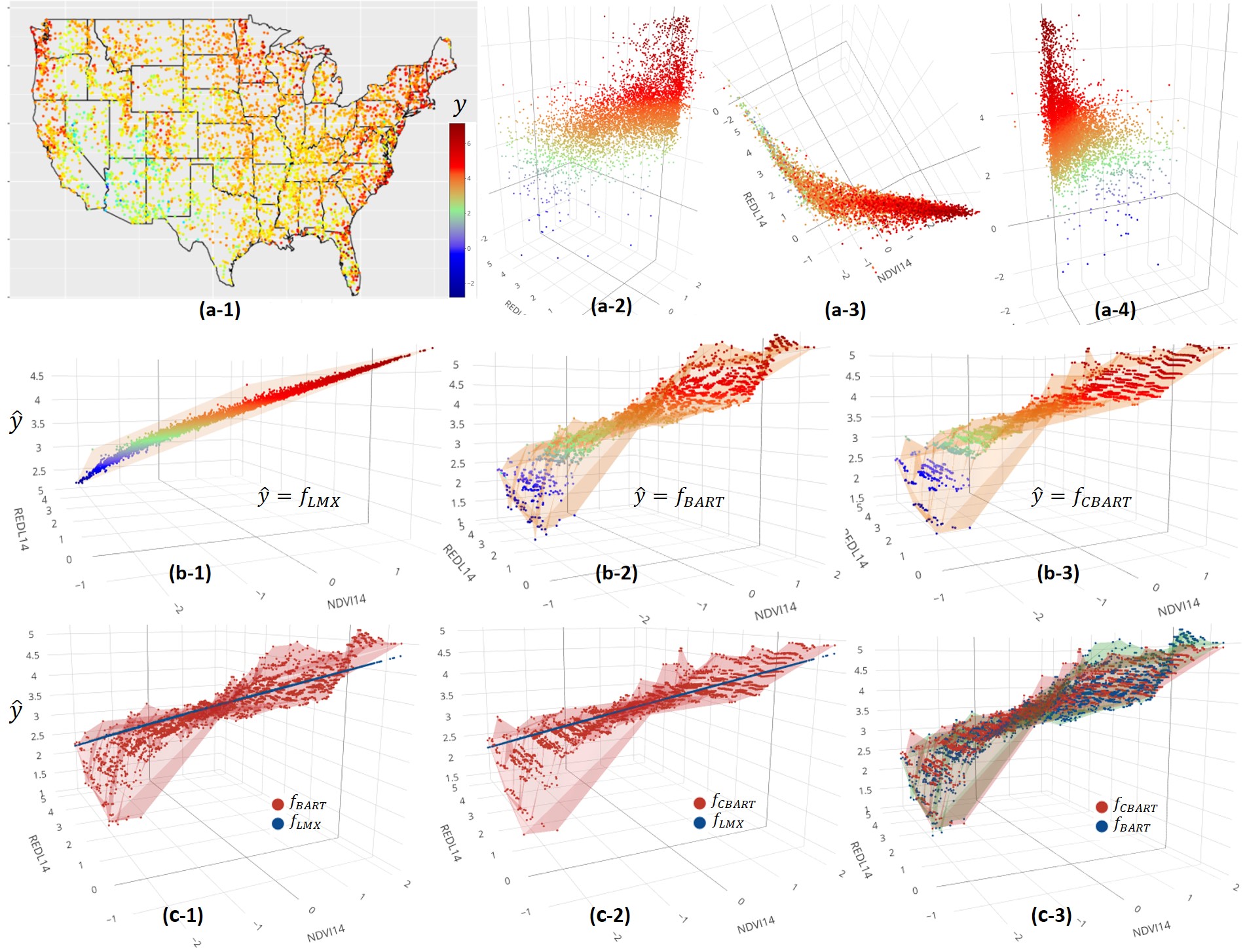
Figure 9: (a-1,2,3,4) The spatial distribution of the response and its relation to the covariates. (b-1,2,3) The fitted $f_{LMX}$, $f_{BART}$ and $f_{CBART}$. (c-1,2,3) The paired comparisons of the three models.

Table 3: Select the optimal maximum likelihood estimators of $\{\sigma^{2},\tau^{2}\}$ by using the minimal value of $|MSE_{real}-MSE_{proposed}|$.

$w_{BART}$	0	0.25	0.5	0.75	1
$|MSE_{real}-MSE_{proposed}|$	0.238	0.212	0.205	0.186	0.195

The parameters that need to be estimated are $\{\sigma^{2},\tau^{2}\}$. We use the method de-meaning with the back comparing and tuning range to estimate these parameters. The tuning range is shown in Table 3. The optimal one is identified by the minimal value of $|MSE_{real}-MSE_{proposed}|$. The corresponding maximum likelihood estimators are $\{\hat{\sigma}^{2},\hat{\tau}^{2}\}=\{0.037,0.417\}$.Using them, we can obtain the $f_{CBART}$. The middle row of Figure 9 shows the fitted $f_{LMX}$, $f_{BART}$, and $f_{CBART}$. The panels in the bottom row of Figure 9 show the paired comparisons of these three models. It is not difficult to find that $f_{CBART}$ lies between $f_{LMX}$ and $f_{BART}$. The MSE (including the GP part for LMX and CBART) of these three models are $MSE_{LMX}=0.74$, $MSE_{CBART}=0.67$, and $MSE_{BART}=0.65$. This indicates that $f_{CBART}$ can capture the nonlinearity of the data while mitigating overfitting.

6 Conclusion

We proposed a novel dummy representation for the single tree in BART and developed CBART accordingly to accommodate correlated errors. CBART could alleviate the overfitting problem and has the potential to obtain a more accurate estimation of the true regression mean function $E[y|x]=f(x)$. Additionally, by combining CBART and Gaussian processes, we constructed the GP-CBART model, which effectively handles time series and spatial data. As demonstrated by simulation studies and real data analysis, GP-CBART has the advantage of capturing non-linearity compared to the linear mixed model and mitigating overfitting compared to BART models. Although we provide three approaches to address the identification and degradation issues in model fitting, further investigation is needed for the full Bayesian solution of GP-CBART.

Appendix A Proofs

Appendix B Marginal likelihood ratio calculation

This approach includes the following three steps.(1) Calculate matrix ABy (22) and (27), we know

$$A=Q+D_{P}^{T}\Sigma_{P}^{-1}D_{P},$$

where $Q=\tau^{-2}I$.$A$ is a symmetric matrix and can be denoted as follows:

$$A=\begin{bmatrix}a_{11}+\tau^{-2}&a_{12}&...&a_{1b}\\ a_{21}&a_{22}+\tau^{-2}&...&a_{2b}\\ \vdots&\vdots&\ddots\\ a_{b1}&a_{b2}&...&a_{bb}+\tau^{-2}\end{bmatrix},$$ (37)

where

$$a_{ji}=a_{ij}=\sum_{h\in\Omega_{i}}\sum_{l\in\Omega_{j}}q_{hl},\hskip 15.0pti\leq j,\hskip 15.0pti,j\in\{1,...,b\}.$$

$\Omega_{i}$ and $\Omega_{j}$ are the index sets of observations that are associated with bottom nodes $i$ and $j$; $q_{hl}$ is the entry at the intersection of $h^{th}$ row and $l^{th}$ column in matrix $\Sigma_{P}^{-1}$ as follows:

$$\Sigma_{P}^{-1}=\begin{bmatrix}q_{11}&q_{12}&...&q_{1n}\\ q_{21}&q_{22}&...&q_{2n}\\ \vdots&\vdots&\ddots\\ q_{n1}&q_{n2}&...&q_{nn}\end{bmatrix}$$

(2) Calculate the block matrix EPluging $A$ into (25), we can get

$$\begin{split}\frac{p(R|D^{i+1})}{p(R|D^{i})}=&\frac{|Q^{i+1}|^{1/2}}{|Q^{i}|^{1/2}}\frac{|A^{i}|^{1/2}}{|A^{i+1}|^{1/2}}\\ &\cdot exp\{\frac{1}{2}R_{P}^{T}\Sigma_{P}^{-1}\underbrace{[D_{P}^{i+1}(A^{i+1})^{-1}(D_{P}^{i+1})^{T}-D_{P}^{i}(A^{i})^{-1}(D_{P}^{i})^{T}]}_{E}\Sigma_{P}^{-1}R_{P}\}.\end{split}$$

To calculate $E$, we need to consider the birth and death operations separately. Without loss of generality, let’s assume that the birth or death operation occurs in the $(i+1)^{th}$ MCMC iteration.BirthIn birth operation, the tree has $b$ bottom nodes at $i^{th}$ iteration and $b+1$ bottom nodes at $(i+1)^{th}$ iteration. The corresponding $(A^{i})^{-1}$ and $(A^{i+1})^{-1}$ are $b\times b$ and $(b+1)\times(b+1)$ matrices. We can denote them by block matrices as follows:

$$(A^{i+1})^{-1}=\begin{bmatrix}V^{i+1}_{11}&V^{i+1}_{12}\\ V^{i+1}_{21}&V^{i+1}_{22}\end{bmatrix},\hskip 15.0pt(A^{i})^{-1}=\begin{bmatrix}V^{i}_{11}&v^{i}_{12}\\ v^{i}_{21}&v^{i}_{22}\end{bmatrix}$$

where, $V^{i+1}_{11}$ and $V^{i}_{11}$ are $(b-1)\times(b-1)$ matrices; $V^{i+1}_{12}=(V^{i+1}_{21})^{T}$ is $(b-1)\times 2$ matrix; $v^{i}_{12}=v^{i}_{21}$ is a $b-1$ column vector; $v^{i}_{22}$ is a scalar.We create a matrix

$$(A^{i})_{ex}^{-1}=\begin{bmatrix}V^{i}_{11}&v^{i}_{12}&v^{i}_{12}\\ v^{i}_{21}&v^{i}_{22}&v^{i}_{22}\\ v^{i}_{21}&v^{i}_{22}&v^{i}_{22}.\end{bmatrix}$$

Let $B=(A^{i+1})^{-1}-(A^{i})_{ex}^{-1}$, then we can get

$$B=\begin{bmatrix}V^{i+1}_{11}-V^{i}_{11}&V^{i+1}_{12}-\begin{bmatrix}v^{i}_{12}&v^{i}_{12}\end{bmatrix}\\ V^{i+1}_{21}-\begin{bmatrix}v^{i}_{21}\\ v^{i}_{21}\end{bmatrix}&V^{i+1}_{22}-\begin{bmatrix}v^{i}_{22}&v^{i}_{22}\\ v^{i}_{22}&v^{i}_{22}\end{bmatrix}\end{bmatrix}=\begin{bmatrix}b_{11}&b_{12}&...&b_{1(b+1)}\\ b_{21}&b_{22}&...&b_{2(b+1)}\\ \vdots&\vdots&\ddots\\ b_{(b+1)1}&b_{(b+1)2}&...&b_{(b+1)(b+1)}.\end{bmatrix}$$

Death
Similar to the birth operation, we have $(A^{i})^{-1}$ and $(A^{i+1})^{-1}$ as follows:

$$(A^{i})^{-1}=\begin{bmatrix}V^{i}_{11}&V^{i}_{12}\\ V^{i}_{21}&V^{i}_{22}\end{bmatrix},\hskip 15.0pt(A^{i+1})^{-1}=\begin{bmatrix}V^{i+1}_{11}&v^{i+1}_{12}\\ v^{i+1}_{21}&v^{i+1}_{22}\end{bmatrix}$$

where $V^{i+1}_{11}$ and $V^{i}_{11}$ are $(b-2)\times(b-2)$ matrices; $V^{i}_{12}=(V^{i}_{21})^{T}$ is $(b-2)\times 2$ matrix; $v^{i+1}_{12}=v^{i+1}_{21}$ is a $b-2$ column vector; $v^{i+1}_{22}$ is a scalar.
Create a matrix

$$(A^{i+1})_{ex}^{-1}=\begin{bmatrix}V^{i+1}_{11}&v^{i+1}_{12}&v^{i+1}_{12}\\ v^{i+1}_{21}&v^{i+1}_{22}&v^{i+1}_{22}\\ v^{i+1}_{21}&v^{i+1}_{22}&v^{i+1}_{22}.\end{bmatrix}$$

In this case, $B=(A^{i+1})_{ex}^{-1}-(A^{i})^{-1}$ as follows:

$$B=\begin{bmatrix}V^{i+1}_{11}-V^{i}_{11}&\begin{bmatrix}v^{i+1}_{12}&v^{i+1}_{12}\end{bmatrix}-V^{i}_{12}\\ \begin{bmatrix}v^{i+1}_{21}\\ v^{i+1}_{21}\end{bmatrix}-V^{i}_{21}&\begin{bmatrix}v^{i+1}_{22}&v^{i+1}_{22}\\ v^{i+1}_{22}&v^{i+1}_{22}\end{bmatrix}-V^{i}_{22}\end{bmatrix}=\begin{bmatrix}b_{11}&b_{12}&...&b_{1b}\\ b_{21}&b_{22}&...&b_{2b}\\ \vdots&\vdots&\ddots\\ b_{b1}&b_{b2}&...&b_{bb}\end{bmatrix}$$

Block matrix E

$$E=D_{P}^{i+1}(A^{i+1})^{-1}(D_{P}^{i+1})^{T}-D_{P}^{i}(A^{i})^{-1}(D_{P}^{i})^{T}=\begin{bmatrix}E_{11}&E_{12}&...&E_{1b^{\prime}}\\ E_{21}&E_{22}&...&E_{2b^{\prime}}\\ \vdots&\vdots&\ddots\\ E_{b^{\prime}1}&E_{b^{\prime}2}&...&E_{b^{\prime}b^{\prime}}\end{bmatrix}$$

where the $b^{\prime}$ in the subscript of the block matrices $E_{ij}$ is

$$b^{\prime}=\begin{cases}b+1,&\text{Birth},\\ b,&\text{Death}.\end{cases}$$

and, each block $E_{ij}$ has a special form as follows:

$$E_{ij}=E_{ji}^{T}=b_{ij}\mathbb{J}_{ij},\hskip 15.0pti\leq j,\hskip 15.0pti,j\in\{1,...,b^{\prime}\}$$

where $b_{ij}$ is the $(i,j)$ entry of matrix $B$ calculated in the birth or death step; $\mathbb{J}_{ij}$ is a card($\Omega_{i}$) $\times$ card($\Omega_{j}$) matrix whose entries are all 1.(3) Calculate marginal likelihood ratioLet’s set

$$R_{P}^{T}\Sigma_{P}^{-1}=\begin{bmatrix}\omega_{1}&\omega_{2}&\ldots&\omega_{b^{\prime}}\end{bmatrix},\hskip 15.0pt\omega_{i}=[\omega_{ij}],\hskip 15.0ptj\in n_{i}$$

and

$$u=R_{P}^{T}\Sigma_{P}^{-1}E\Sigma_{P}^{-1}R_{P}.$$

Then, $u$ can be calculated as follows:

$$\begin{split}u&=\begin{bmatrix}\omega_{1}&\omega_{2}&\ldots&\omega_{b^{\prime}}\end{bmatrix}E\begin{bmatrix}\omega_{1}^{T}\\ \omega_{2}^{T}\\ \vdots\\ \omega_{b^{\prime}}^{T}\end{bmatrix}\\ &=\sum_{i=1}^{b^{\prime}}\sum_{j=1}^{b^{\prime}}\omega_{i}E_{ij}\omega_{j}^{T}\\ &=\sum_{i=1}^{b^{\prime}}\sum_{j=1}^{b^{\prime}}(\omega_{i}\mathbb{J}_{ij}\omega_{j}^{T})b_{ij}\\ &=\sum_{i=1}^{b^{\prime}}\sum_{j=1}^{b^{\prime}}[(\sum_{h\in n_{i}}\omega_{ih})(\sum_{l\in n_{j}}\omega_{jl})b_{ij}].\end{split}$$

Finally, we can get the marginal likelihood ratio as follows:

$$\frac{p(R|D^{i+1})}{p(R|D^{i})}=\begin{cases}\tau^{-1}\frac{|A^{i}|}{|A^{i+1}|}exp\{\frac{1}{2}u\}\hskip 25.0ptBirth\\ \tau\frac{|A^{i}|}{|A^{i+1}|}exp\{\frac{1}{2}u\}\hskip 35.0ptDeath.\end{cases}$$

References

- Brahim-Belhouari and Bermak (2004) Brahim-Belhouari, S. and A. Bermak (2004). Gaussian process for nonstationary time series prediction. Computational Statistics & Data Analysis 47(4), 705–712.
- Chipman et al. (2006) Chipman, H., E. George, and R. Mcculloch (2006). Bayesian ensemble learning. In B. Schölkopf, J. Platt, and T. Hoffman (Eds.), Advances in Neural Information Processing Systems, Volume 19. MIT Press.
- Chipman et al. (1998) Chipman, H. A., E. I. George, and R. E. McCulloch (1998). Bayesian cart model search. Journal of the American Statistical Association 93(443), 935–948.
- Chipman et al. (2010) Chipman, H. A., E. I. George, and R. E. McCulloch (2010). Bart: Bayesian additive regression trees. The Annals of Applied Statistics 4, 266–298.
- Cressie (1993) Cressie, N. (1993). Statistics for Spatial Data, pp. 1–26. John Wiley & Sons, Ltd.
- Cressie (2015) Cressie, N. (2015). Statistics for Spatial Data. Wiley Series in Probability and Statistics. Wiley.
- Datta et al. (2016) Datta, A., S. Banerjee, A. O. Finley, and A. E. Gelfand (2016). Hierarchical nearest-neighbor gaussian process models for large geostatistical datasets. Journal of the American Statistical Association 111(514), 800–812.
- Finley et al. (2019) Finley, A. O., A. Datta, B. D. Cook, D. C. Morton, H. E. Andersen, and S. Banerjee (2019). Efficient algorithms for bayesian nearest neighbor gaussian processes. Journal of Computational and Graphical Statistics 28(2), 401–414.
- George et al. (2019) George, E., P. Laud, B. Logan, R. McCulloch, and R. Sparapani (2019). Fully Nonparametric Bayesian Additive Regression Trees. In I. Jeliazkov and J. L. Tobias (Eds.), Topics in Identification, Limited Dependent Variables, Partial Observability, Experimentation, and Flexible Modeling: Part B, Volume 40 of Advances in Econometrics, pp. 89–110. Emerald Publishing Ltd.
- Goldberger (1962) Goldberger, A. S. (1962). Best linear unbiased prediction in the generalized linear regression model. Journal of the American Statistical Association 57(298), 369–375.
- Hackbusch (2015) Hackbusch, W. (2015). Hierarchical Matrices: Algorithms and Analysis (1st ed.). Springer Publishing Company, Incorporated.
- Hastie and Tibshirani (2000) Hastie, T. and R. Tibshirani (2000). Bayesian backfitting. Statistical Science 15(3), 196–213.
- Hill et al. (2020) Hill, J. L., A. R. Linero, and J. Murray (2020). Bayesian additive regression trees: A review and look forward. Annual Review of Statistics and Its Application.
- Krige (1951) Krige, d. g. (1951). A Statistical Approach to Some Mine Valuation and Allied Problems on the Witwatersrand.
- Lin et al. (2011) Lin, L., J. Lu, and L. Ying (2011). Fast construction of hierarchical matrix representation from matrix–vector multiplication. Journal of Computational Physics 230(10), 4071–4087.
- Litvinenko et al. (2019) Litvinenko, A., Y. Sun, M. G. Genton, and D. E. Keyes (2019). Likelihood approximation with hierarchical matrices for large spatial datasets. Computational Statistics & Data Analysis 137, 115–132.
- Lu et al. (2022) Lu, X., S. Saul, and C. Jenkins (2022). Statistical methods for predicting the spatial abundance of reef fish species. Ecological Informatics 69, 101624.
- Nychka et al. (2017) Nychka, D., R. Furrer, J. Paige, and S. Sain (2017). fields: Tools for spatial data. R package version 10.3.
- Pebesma (2006) Pebesma, E. J. (2006). The role of external variables and gis databases in geostatistical analysis. Transactions in GIS 10(4), 615–632.
- Piegorsch et al. (2022) Piegorsch, W. W., R. A. Levine, H. H. Zhang, and T. C. M. Lee (2022). Compuatational Statistics in Data Science. Wiley.
- Pratola et al. (2020) Pratola, M. T., H. A. Chipman, E. I. George, and R. E. McCulloch (2020). Heteroscedastic bart via multiplicative regression trees. Journal of Computational and Graphical Statistics 29(2), 405–417.
- Rasmussen and Williams (2005) Rasmussen, C. E. and C. K. I. Williams (2005, 11). Gaussian Processes for Machine Learning. The MIT Press.
- Roberts et al. (2012) Roberts, S. J., M. A. Osborne, M. Ebden, S. Reece, N. P. Gibson, and S. Aigrain (2012). Gaussian processes for timeseries modelling.
- Stein and Corsten (1991) Stein, A. and L. C. A. Corsten (1991). Universal kriging and cokriging as a regression procedure. Biometrics 47(2), 575–587.