Generalized Additive Forecasting Mortality

Abstract

This study introduces a novel Generalized Additive Mixed Model (GAMM) for mortality modelling, employing mortality covariates $k_{t}$ and $k_{ct}$ as proposed by Dastranj- Kolář (DK-LME). The GAMM effectively predicts age-specific death rates (ASDRs) in both single and multi-population contexts. Empirical evaluations using data from the Human Mortality Database (HMD) demonstrate the model’s exceptional performance in accurately capturing observed mortality rates. In the DK-LME model, the relationship between log ASDRs, and $k_{t}$ did not provide a perfect fit. Our study shows that the GAMM addresses this limitation. Additionally, as discussed in the DK-LME model, ASDRs represent longitudinal data. The GAMM offers a suitable alternative to the DK-LME model for modelling and forecasting mortality rates. We will compare the forecast accuracy of the GAMM with both the DK-LME and Li-Lee models in multi-population scenarios, as well as with LC models in single population scenarios. Comparative analyses highlight the GAMM’s superior sample fitting and out-of-sample forecasting performance, positioning it as a promising tool for mortality modelling and forecasting.

1 Introduction

An ASDR is a mortality rate in a particular age group. For each population, ASDRs are collected sequentially in different years. Mortality rates from the same age group are usually more similar than rates from other age groups. That means rates from the same age group are related to one another. Therefore, ASDRs form a longitudinal dataset (i.e. repeated measurements over time ( Frees et al. 2004, Antonio and Beirlant 2007)) where observations within each age group are correlated.

LME models are particularly valuable for analyzing longitudinal data, such as ASDRs collected over time from different populations. By combining both fixed effects and random effects, LME models enable the capturing of both population-level trends and individual-level variations within the data. Fixed effects help uncover general patterns and associations between mortality rates and various factors of interest, such as age and gender. On the other hand, random effects address the correlations and dependencies present within specific groups, accounting for the similarities among observations within the same age group. In the context of mortality forecasting, LME models offer several advantages and insights. Their ability to integrate fixed and random effects enables a comprehensive understanding of the underlying factors influencing mortality rates. They can capture both overall population-level trends and specific variations within subgroups. Additionally, LME models are well-suited for handling the longitudinal nature of mortality data collected sequentially over time. This allows for the incorporation of temporal dependencies and the exploration of trends and changes in mortality rates across different time periods.

Dastranj and Kolár (2023) introduce an innovative approach using linear mixed-effects (DK-LME) models for the analysis and prediction of mortality rates. This study’s key contributions include the integration of age, the interaction between gender and age, and their interactions with the predictors $k_{t}$ and $k_{ct}$, and cohort as fixed effects. Furthermore, we have incorporated additional random effects to account for variations in the intercept, predictor coefficients, and cohort effects among different age groups of females and males across various countries. We conducted a comparative analysis by assessing the performance of the DK-LME model against the Lee-Carter (LC) models fitted to individual populations. Additionally, we evaluated the predictive accuracy of the LME model in comparison to the Lee-Li (LL) model. Our findings demonstrate that the LME model offers a more precise representation of observed mortality rates within the Human Mortality Database (HMD). It exhibits robustness in selecting calibration rates and outperforms the LC and LL models. These results highlight the suitability of the LME model as a framework for modeling and forecasting mortality trends. Therefore, Dastranj and Kolár (2023) highlights the significance of utilizing LME models in mortality forecasting due to their capacity to combine fixed and random effects. This approach captures both broad trends and nuanced variations within age groups, genders, and countries. By accounting for data correlations and temporal dependencies, LME models offer an improved and more accurate analysis of mortality trends, leading to enhanced predictions and valuable insights for understanding and forecasting mortality patterns.

The DK-LME model utilizes log ASDRs plotted against the mortality covariate $k_{t}$ to explore mortality variations, particularly across country-gender aggregates and within 24 distinct age groups. While the LME model offers valuable insights, it has its limitations. Notably, the relationship between $y_{cgxt}$ and $k_{t}$ in the DK-LME model did not yield a perfect fit. To address this limitation, the authors introduces a GAMM (see Wood (2017); Hastie (2017)). The GAMM aims to combine the strengths of the LME model while addressing its shortcomings by effectively capturing any nonlinear relationships between log ASDRs and the mortality covariate $k_{t}$. Hilton et al. (2019) and Hall and Friel (2011) have previously employed generalized additive modelling in the projection of mortality rates. This approach has demonstrated its utility and effectiveness in similar contexts.

GAMMs can be considered a generalization of LME models, with the addition of the flexibility to model nonlinear relationships using additive functions (see Wood (2017)). LMMs are a type of statistical model used to analyze data with both fixed effects (variables we are interested in studying) and random effects (variables that are not of primary interest but are included due to their impact on the data). LME models assume a linear relationship between the response variable and predictor variables. They are commonly used in various fields, including social sciences, biology, and economics. The fixed effects are modeled linearly, and the random effects account for variability due to unobserved factors. GAMMs extend the concept of LME models by allowing for the inclusion of nonlinear relationships between predictors and the response variable. They can handle not only linear but also nonlinear effects of predictors on the response. This is achieved through the use of additive functions, which means that each predictor can have a separate, flexible smooth function that captures its effect on the response. These smooth functions are often implemented using techniques like splines. GAMMs encompass the capabilities of LMMs by incorporating random effects and adding the flexibility to model nonlinear relationships using smooth functions. Therefore, we can view GAMMs as a generalization of LME models that provides a broader scope of modelling options. This added flexibility makes GAMMs especially useful when relationships between variables are not strictly linear and may exhibit more complex patterns.

In GAMMs, smooth functions are a crucial component that allows for the modelling of nonlinear relationships between predictors and the response variable. These smooth functions are used to capture complex and flexible patterns in the data that may not be well-modelled using simple linear relationships. Smooth functions are implemented using various mathematical techniques, and one common approach is through the use of splines. While splines are a common technique to implement smooth functions, there are other approaches as well: B-splines are piecewise polynomial functions that are defined over intervals (segments). The overall smooth function is constructed by combining multiple B-splines with different coefficients at each segment. The coefficients control the shape of the curve, and they are estimated from the data. Natural splines are Similar to B-splines, but they impose additional constraints at the endpoints to ensure smoothness. This can be particularly useful when we want a smooth curve that does not oscillate too much at the edges. P-splines (penalized splines) combine the flexibility of splines with a regularization term that helps prevent overfitting. They use a penalty term on the coefficients of the spline to control the smoothness of the curve. This approach allows for automatic selection of the number and placement of knots while avoiding excessive wiggles in the curve. Smoothing splines are similar to B-splines but are obtained by minimizing a penalized residual sum of squares. They find the smoothest curve that fits the data within certain constraints. Thin plate splines (Wood 2003) are a type of spline function that can be used to create smooth surfaces in multidimensional space. They are particularly useful when we have multiple predictor variables and want to capture complex interactions and nonlinear relationships among them. Gaussian processes are a probabilistic framework that models the relationship between variables by assuming that any set of variables follows a joint Gaussian distribution. They allow for very flexible modelling of nonlinear relationships and can capture uncertainties in predictions. Local regression methods, like LOESS (Locally Weighted Scatterplot Smoothing), fit a separate regression function to each data point by giving more weight to nearby points. This allows for capturing local trends in the data. These techniques provide various ways to implement smooth functions in GAMMs. The choice of technique depends on factors like the complexity of the data, the desired smoothness of the curves, computational efficiency, and the specific goals of the analysis. The overarching goal is to capture the underlying patterns in the data while avoiding overfitting and achieving good generalization to new data. For one-dimensional predictors, such as continuous variables, the default smooth function technique in mgcv often employs cubic regression splines. Cubic splines are piecewise-defined cubic polynomials that are joined together at specific points called knots. These knots are chosen automatically based on the data distribution. The cubic nature of the splines ensures smoothness up to the second derivative, resulting in smooth curves that can capture nonlinear relationships. For higher-dimensional predictors or interactions between predictors, mgcv uses tensor product smooths. Tensor product smooths allow for the creation of smooth surfaces in multidimensional predictor spaces. These surfaces capture interactions and nonlinear relationships among the predictors. The smoothing is done in a way that ensures smoothness across all dimensions, while avoiding overly complex and wiggly curves

When using the mgcv package (Wood and Wood ) in R to fit GAMs or GAMMs, the default smooth function technique is based on cubic regression splines for one-dimensional predictors and tensor product smooths for higher-dimensional predictors. The package uses these techniques to create smooth functions that capture the relationships between predictors and the response variable.

The examination of ASDR trends concerning the mortality covariate $k_{t}$ unveils evident non-linear patterns. To effectively capture these intricacies, we employ GAM as our approach for analyzing mortality data. GAM, initially introduced by Hastie and Tibshirani (Hastie and Tibshirani 1986) and further refined by Wood in 2006, is a versatile regression technique that accommodates both linear and non-linear relationships between the dependent variable (ASDRs) and the independent variables (mortality covariate $k_{t}$ and $k_{ct}$). In contrast to traditional linear mixed effects methods, GAMMs provide us with the capability to model intricate interactions and dependencies between ASDRs and $k_{t}$, as well as between ASDRs and $k_{ct}$, resulting in more accurate modeling. This enhanced flexibility allows for a comprehensive understanding of the intricate associations within our data, leading to more precise and insightful conclusions in our study.

The paper is organized as follows: In Section 2, we introduce the GAMM for ASDRs in a multi-population dataset. We apply the GAMM to a dataset encompassing four populations for the period spanning 1961 to 2010. Subsequently, we use the model to forecast mortality rates for these four populations up to the year 2019. In Section 3, we extend our focus to the GAMM’s application within single population datasets. Specifically, we introduce the GAMM for ASDRs in single populations and apply it to fifty-eight individual population datasets sourced from the HMD (HMD 2023). These datasets contain observations predating the year 2000, and we utilize the GAMM to project mortality rates from 2000 to 2019. Finally, Section 4 serves as the conclusion, offering a critical discussion of the GAMM’s performance and its broader implications.

2 Modelling ASDRs Across Multiple Populations

Age-specific mortality patterns provide a unique window into the complex web of factors influencing mortality rates among various age groups. Think of these patterns as a kind of "mortality fingerprint," offering insights into the specific health challenges and vulnerabilities faced by people of different ages. While numerical analyses provide valuable insights, the art of data visualization unveils an additional layer of complexity and clarity. To fully grasp how mortality is distributed across different age groups within a population, it is crucial to examine mortality data carefully. Let us consider Figure 1 as an example, where ASDRs are portrayed over a span of five decades for two countries. Each curve, shown on a logarithmic scale, tells a unique story of mortality over time. What becomes evident is a compelling tale of progress, as we witness a consistent decline in mortality rates, suggesting that, on average, people are enjoying longer lives. What is most fascinating, though, is the remarkable similarity in how mortality rates change, both within specific age groups and across diverse populations. Even when comparing different regions and demographics, a surprising consistency in the trajectory of mortality rates is found. Yet, amidst this regularity, the red curves at the center of Figure 1, representing infant mortality, stand out clearly, displaying significant fluctuations. This finding highlights the profound impact of infant health on the broader landscape of mortality. In essence, these age-specific patterns and temporal trends go beyond just mortality statistics; they tell a story of human resilience and adaptation in the face of evolving health challenges. By finding the regularity in both age patterns and trends over time, we conclude that the population age structure reveals a consistent and robust internal pattern, indicative of the broader health and societal factors at play in shaping longevity and mortality rates. Understanding these patterns extends beyond mere data analysis; it is an exploration of the human experience and the strategies societies employ to ensure longer, healthier lives.

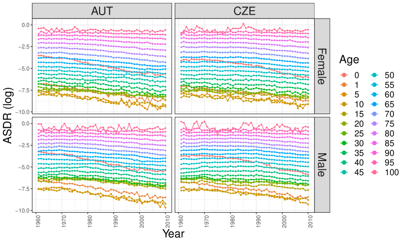
Figure 1: ASDRs across four populations from 1961 to 2010.

In Figures 2, a distinct insight emerges through the representation of the thick black curve, symbolizing $k_{t}$. This curve is derived from the logarithmic average of mortality rates spanning various age groups. Specifically, for instance, $k_{1961}$ reflects the average ASDRs for the year 1961. This aggregated curve, $k_{t}$, essentially captures the overarching trajectory of age-specific mortality rates within the dataset encompassing four different populations. However, a closer examination of the data reveals a noteworthy observation: the trends in mortality rates exhibit substantial diversity across age groups within individual countries. This disparity becomes evident when comparing the ASDRs against the average curve (the black curve), as they demonstrate significant deviations from each other.

Interestingly, the disparities within individual countries stand in contrast to the striking similarity observed in mortality rates among the same age groups across different populations. This pattern underscores the presence of consistent trends, irrespective of national boundaries. The commonality in mortality rate patterns at corresponding ages highlights a shared underlying factor, possibly linked to universal factors like biological aging processes or common health influences. This intriguing finding points toward the influence of intrinsic, age-related factors on mortality rates, which hold sway across various populations.

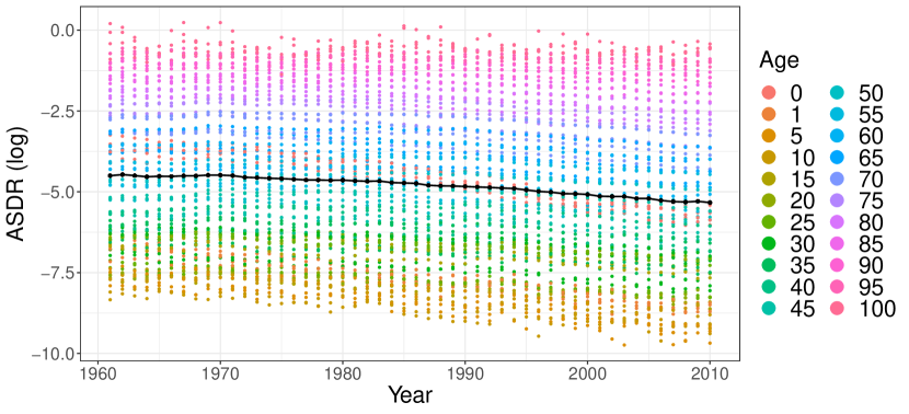
Figure 2: Average log mortality rates ($k_{t}$) across the four populations and all age groups (1961-2010). The thick black curve in this plot represents $k_{t}$, which is the average of log mortality rates across the four distinct populations and all age groups spanning the period from 1961 to 2010. $k_{t}$ serves as a comprehensive measure of the overall mortality trend during this five-decade interval, offering valuable insights into the collective impact on mortality rates across diverse populations and age groups.

In Figure 3, the bold blue and red curves represent a variable denoted as $k_{ct}$. This variable is calculated by averaging the logarithm of mortality rates over two distinct age ranges: ages 0 to 40 and ages 45 to 100. This division is employed to emphasize the specific influence of external factors on mortality rates within different age groups. Historical data reveals a noteworthy pattern: mortality rates for individuals in younger age groups, typically up to 40 or 50 years old, exhibit significant fluctuations during various time periods. These fluctuations are primarily attributed to external factors and societal changes. Certain influences, such as the prevalence of conditions like AIDS, substance abuse, and increased violence, have a notably more pronounced impact on the younger demographic. These factors have played a substantial role in shaping mortality trends (see Plat 2009). Consequently, the inclusion of the factor $k_{ct}$ in the GAMM aims to provide a more comprehensive explanation of these dynamic influences, particularly their amplified effects on younger age groups. It is evident from the data that, for the specified age groups [0,40] and [45,100], the values of the blue and red curves for Austria (AUT) are consistently lower than the values of the blue and red curves for the Czech Republic (CZE). This indicates that, on average, mortality rates in Austria are lower than those in the Czech Republic for these age groups. Integrating the variable $k_{ct}$ into the GAMM allows us to effectively capture and account for the observed variations across these two countries.

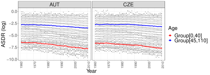
Figure 3: $k_{ct}$ Plot: The bold blue and red curves elegantly reveal the variable, $k_{ct}$, calculated by averaging the logarithm of mortality rates over two distinct age ranges: ages 0 to 40 and ages 45 to 100. This division serves as a powerful lens, shedding light on the distinct impact of external factors on mortality rates.

The method of GAMMs is now well established. Let $m_{c,g,x,t}$ denote the ASDR at age $x$ and time $t$ of gender $g$ in country $c$, for $c=$ $1,2,\cdots,M$; $g=1,2$; $x=0,1,\cdots,\omega$; and $t=0,1,\cdots,T$. Let $y_{cgxt}=\log(m_{c,g,x,t})$. Let $k_{ct}$ represent the average of $y_{cgxt}$ for two distinct age range groups: the average for age groups 0 to 40 and the average for age groups 41 to $\omega$, encompassing both females and males in country $c$ at time $t$. Additionally, let $k_{t}$ denote the average of $y_{cgxt}$ at time $t$ across all age groups in all countries and genders:

$$k_{ct}= \begin{cases}k_{ct}^{[0,40]}&\text{if}\ x\in[0,40],\\ k_{ct}^{[41,\omega]}&{\rm otherwise},\end{cases};\qquad k_{t}=\dfrac{\sum\limits_{c=1}^{M}\sum\limits_{g=1}^{2}\sum\limits_{x=0}^{\omega}y_{cgxt}}{2M(\omega+1)},$$ (1)

for $c=1,2,\cdots,M$, and $t=0,1,\cdots,T$, where

$$k_{ct}^{[0,40]}=\dfrac{\sum\limits_{g=1}^{2}\sum\limits_{x=0}^{40}y_{cgxt}}{2(41)},\qquad k_{ct}^{[41,\omega]}=\dfrac{\sum\limits_{g=1}^{2}\sum\limits_{x=41}^{\omega}y_{cgxt}}{2(\omega-40)},$$

for $c=1,2,\cdots,M$, and $t=0,1,\cdots,T$. Within our GAMM, we will incorporate two pivotal covariates, namely $k_{ct}$ and $k_{t}$, which originally stem from the DK-LME model. These covariates play a vital role in unraveling mortality patterns across different age groups and countries. To forecast their future values, we will employ a statistical method known as random walks with drift. Our predictions will encompass $k_{ct}$ values for age groups spanning from $0$ to $40$ in each country, providing insights into mortality trends in younger populations. Additionally, we will also predict $k_{ct}$ values for age groups from $41$ to $\omega$, offering a perspective on mortality patterns in older age groups. Additionally, our model will also include forecasting the future values of $k_{t}$, an essential component borrowed from the DK-LME model, to provide a comprehensive view of mortality dynamics across different age groups and countries within the GAMM framework.

Figure 3 displays logarithmically transformed ASDR trajectories, labeled as $y_{cgxt}$, in relation to the mortality covariate $k_{t}$. These trajectories are observed across distinct age groups, specifically 50 and 60, within each of the four populations that constitute the focus of our study. The plot illustrating the relationship between the response variable and the covariate is central to our approach in this paper. Our capacity to achieve superior fitting within this plot directly results in reduced residuals, thereby enhancing the modelling and forecasting ASDRs. Furthermore, when introducing alternative statistical models for the ASDRs dataset, it is paramount to consider it as an initial step to assess how well the proposed model can capture the relationship between $y$ and $k_{t}$.

In the analysis of mortality data, it has become evident that the logarithmically transformed ASDR trajectories exhibit pronounced nonlinearity concerning the mortality covariate $k_{t}$ (see Figure 4). This inherent nonlinearity in the relationship between the dependent variable, log ASDR, and the independent variable, the mortality covariate, presents a complex analytical challenge. Traditional linear models struggle to accommodate these complexities, necessitating the adoption of a more sophisticated approach. To address this challenge, we have chosen to employ GAMMs. GAMMs are a powerful extension of the conventional GAMs framework, enriched by the incorporation of random effects. This augmentation equips GAMMs with the unique capability to effectively handle scenarios involving correlated and clustered responses. GAMMs excel in capturing nuanced relationships within the data, particularly when dealing with structured dependencies found in longitudinal data and research designs that incorporate repeated measurements. Their adaptability sets them apart, allowing us to move beyond the limitations of linear regression. Unlike traditional linear regression models, which are confined to modeling linear associations between the dependent variable ($y_{cgxt}$) and the independent variable ($k_{t}$), GAMMs proficiently accommodate non-linear associations. This adaptability is pivotal as it enables us to encapsulate intricate correlations and interactions intrinsic to the dataset.

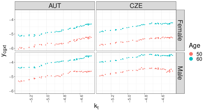
Figure 4: Exploring the relationship between logarithmically transformed ASDR trajectories ($y_{cgxt}$) and the mortality covariate ($k_{t}$) across the four populations (1961-2010). This plot investigates the connection between $y_{cgxt}$, representing logarithmically transformed ASDR trajectories, and the mortality covariate $k_{t}$ across the four populations during the period of 1961-2010. These trajectories reveal significant nonlinearity, underscoring the complexity of the association between log mortality and the covariate $k_{t}$.

2.1 The Model Formulation

The command to fit a GAM for an individual age group using the bam (Wood et al. 2015) function from the mgcv package can be stated as follows:

⬇

1model = bam(y $\sim$ age+gender:age+

2 s(kct,bs="ts")+

3 s(kct,by=gender:age,bs="ts")+

4 s(cohort,bs="ts") +

5 s(country:gender:age,bs="re") +

6 s(kt,country:gender:age,bs="fs",m=1)+

7 s(cohort,country:gender:age,bs="fs",m=1),

8 data=ASDRs)

Listing 1: A GAMM for ASDRs in multiple populations.

The interpretation of this specific GAMM specification is as follows:

The age term in the model serves as an intercept for different age groups. It captures the baseline or constant effect of each age category on the response variable when all other factors are held constant. It provides a reference point for interpreting the impact of age categories. The gender:age term plays a vital role in capturing intercepts for each age group and, within each age group, for each gender category. This term allows for distinct baseline values for the response variable based on both age and gender. It identifies and accounts for constant (intercept) differences among these age groups and gender combinations. s($k_{ct}$, bs="ts"): this term uses a thin-plate spline (bs="ts") to model the relationship between the predictor variable $k_{ct}$ and the response variable $y_{cgxt}$. The thin-plate spline is a non-linear and low-rank smoother that allows for flexible and adaptive modeling of the relationship. It captures complex and non-linear patterns in the data without requiring the specification of knots. The smoothing parameter controls the degree of smoothness, allowing the model to adapt to the data patterns. s($k_{ct}$, by=gender:age, bs="ts"): this term represents a smooth function of $k_{ct}$ while allowing the smoothness to vary based on the interaction of the factor variables gender and age. It allows for different smooth curves for $k_{ct}$ for different combinations of gender and age, capturing complex and non-linear relationships. s(cohort, bs="ts"): this term models a smooth function of the factor variable cohort using a thin-plate spline basis. It captures the non-linear relationship between cohort and the response variable $y_{cgxt}$, providing flexibility to model complex patterns. s(country:gender:age, bs="re"): this term models a random effect for the combination of factor variables country, gender, and age using the "re" (random effects) basis. It captures random variability in the relationship between the response variable $y_{cgxt}$ and these factor combinations. This term allows for variation in intercepts among different levels of the factor combinations. s($k_{t}$, country:gender:age, bs="fs", m=1): this term models a factor-smooth interaction for the variable $k_{t}$ while considering the combination of country, gender, and age. It allows the smooth effect of $k_{t}$ to vary across different levels of this combination while maintaining a common smoothness constraint. s(cohort, country:gender:age, bs="fs", m=1): this term models a factor-smooth interaction for the variable cohort while considering the combination of country, gender, and age. It allows the smooth effect of cohort to vary across different levels of this combination while maintaining a common smoothness constraint.

After fitting the model, we conducted a thorough examination of the residuals to assess the presence of heteroskedasticity, which refers to the unequal variance of residuals across a range of observed values. Heteroskedasticity can manifest as a non-uniform scatter of residuals, impacting the reliability of the model.

Our analysis revealed that the residuals exhibited nonnormality and heteroscedasticity, indicating that the variance of residuals was not consistent across different predicted values. To address this issue, we employed a data-cleaning procedure by excluding data points with absolute residuals greater than 0.1, signifying instances where the predicted and actual values diverged significantly. Subsequently, we re-estimated the model using this refined dataset, which typically retained about $85\%$ of the original data. This procedure resulted in improved characteristics of the residuals.

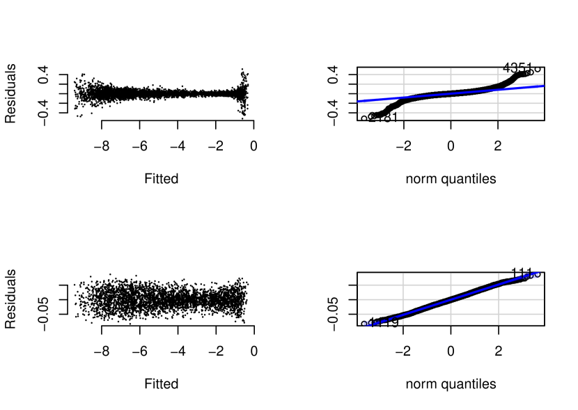
Figure 5: The set of four plots above serves to examine various aspects of the GAMM’s residuals. The top row features the initial two plots, showcasing the residuals against the model’s fitted values and a Quantile-Quantile (QQ) plot of the raw residuals from the GAMM before any corrections were applied. These visualizations unveil deviations from linearity in the residual pattern and raise concerns about the normality of the residuals across the four populations. In contrast, the two plots in the bottom row represent the residuals versus the fitted values and the QQ plot of the residuals after appropriate correction. In these plots, the QQ plot indicates that the residuals’ distribution conforms more closely to a normal distribution. The majority of data points align reasonably well along the reference line, suggesting improved normality. Furthermore, in the second plot of residuals versus fitted values after correction, we observe relatively consistent variance across the entire range of fitted values. Therefore, the corrected GAMM exhibits a more favorable residual pattern, with fewer deviations from linearity and improved adherence to the assumptions of normality. Additionally, the constant variance across the fitted values range after correction indicates that the model’s performance has been enhanced.

All findings presented in this paper are derived from the model post-critique, following the data point exclusion and model refitting. This approach enhances the rigor of our results by reducing the risk of attributing significance to effects driven by data points that do not align with the model’s assumptions.

The residual autocorrelation function (ACF) plot plays a pivotal role in the evaluation of our GAMM for mortality rates (see Figure 6). This plot provides valuable insights into the presence of any remaining patterns or serial correlation in the model residuals, which can significantly impact the reliability of our modelling approach. The ACF plot, as illustrated in Figure 6, presents the autocorrelation coefficients at various time lags. In our analysis, we observe that the coefficient at the first lag is approximately - 0.09. This specific value at the first lag indicates the extent of correlation between the residuals at the current time point and those at the preceding time point. With a value of $-0.09$, this correlation is relatively weak and negative, signifying a modest association between the residuals at lag 1 and those at lag 0. The relatively low autocorrelation value at the first lag implies that there is limited residual correlation between consecutive time points. In practical terms, this suggests that our model has capably captured and accounted for the majority of temporal dependencies in the mortality rate data. Consequently, it indicates that there are no substantial remaining patterns or serial correlations within the model residuals, thereby assuring us that these residual correlations are unlikely to pose issues for the model’s accuracy. Encouragingly, this pattern of low and negligible autocorrelation values at higher lags is consistent. These findings indicate that our model has effectively accommodated and addressed the temporal dependencies in the mortality rate data across various lags. It is essential to underscore the significance of comprehending and addressing the ACF plot, as it enables us to pinpoint any potential model inadequacies. In our specific context, it is imperative to emphasize that our GAMM for mortality rates is well-fitted, given the proximity of the majority of autocorrelation values in the residuals to zero. This proximity suggests minimal residual correlation, confirming the appropriateness of our model’s assumptions regarding temporal dependence.

Considering the insights derived from Figure 5, which encompasses the QQ plot confirming normality assumptions and the homoskedasticity assessment, alongside the ACF plot, we can affirm the comprehensive robustness and validity of our mortality rate model. The QQ plot ensures that our residuals adhere to the normality assumption, while the homoskedasticity assessment confirms consistent variance across different levels or time points. The ACF plot, with its low autocorrelation values, demonstrates that the model effectively addresses temporal dependencies. Together, these diagnostic tools provide a thorough evaluation of the model’s reliability, supporting its suitability for our analysis.

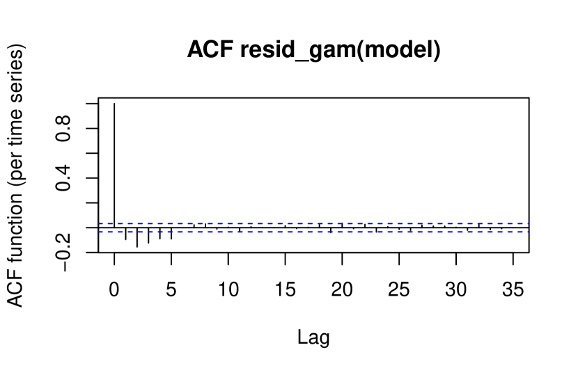
Figure 6: The residual Autocorrelation Function (ACF) plot. It offers invaluable insights into any serial correlation present in the residuals of our model, which could significantly impact the reliability and accuracy of our modelling approach. In the ACF plot, we examine the autocorrelation coefficients at various time lags. It allows us to observe how well the model captures any temporal dependencies or correlations in the data. The coefficient at the first lag, which is approximately -0.09, represents the correlation between the residuals at the current time point and those at the immediate preceding time point.

Figure 7 displays the smoothing functions that have been incorporated into our model.

s($k_{ct}$, bs="ts"): this smoothing function exhibits a simple linear relationship between the predictor variable, $k_{ct}$, and the response variable, $y_{cgxt}$. The curve is essentially a straight line, indicating a straightforward linear effect. The confidence intervals around this smooth curve are relatively narrow, suggesting a high level of confidence in the estimated relationship. The choice of the thin-plate regression spline basis (bs="ts") implies a flexible yet smooth representation of the effect, where the smoothing parameter adjusts the degree of flexibility. The P-value associated with this smooth term is exceptionally low, indicative of extreme statistical significance, reinforcing the strong linear relationship between $k_{ct}$ and $y_{cgxt}$.

s($k_{ct}$, by=gender:age, bs="ts"): this smoothing function extends the model to consider the interaction of gender and age with $k_{ct}$, resulting in a linear relationship for each age group and gender in each country. Compared to the previous plot, the confidence intervals are wider, reflecting increased uncertainty, likely due to the added complexity introduced by the interaction terms. While the P-values vary across different age groups, some show statistical significance, and the decision to retain this term is motivated by the goal of maintaining consistency in the modeling approach for all age groups and genders in the two countries.

s(cohort, bs="ts"): this smoothing function portrays a nonlinear relationship between the predictor variable cohort (year of birth) and the response variable $y_{cgxt}$. The curve is more intricate and captures the complex relationship between these two variables. The x-axis represents the cohort (year of birth), and the y-axis represents the estimated effect of cohort on $y_{cgxt}$. The choice of thin-plate regression spline basis (bs="ts") allows for flexible modeling, and the smoothing parameter controls the degree of flexibility, accommodating potentially non-linear effects. This curve reveals significant features and wiggles, indicating that the effect of cohort is more nuanced and not adequately explained by a simple linear relationship.

s($k_{t}$, country:gender:age, bs="fs", m=1): the presence of wiggles and features in the smooth plot for s($k_{t}$, country:gender:age, bs="fs", m=1) suggests that the effect of $k_{t}$ is not adequately captured by a simple linear model. Instead, its relationship with the response variable is more complex and likely exhibits non-linear patterns. The wiggles and features in the plot indicate that there are variations in the effect of $k_{t}$ across different levels of the combination of country, gender, and age. The low P-value associated with this term is strikingly low, underscoring the strong statistical significance of the effect of $k_{t}$. This suggests that the non-linear relationship it represents is highly significant in explaining the variability in the response variable.

s(cohort, country:gender:age, bs="fs", m=1): similarly, the smooth plot for s(cohort, country:gender:age, bs="fs", m=1) displays wiggles and features, indicating that the relationship between cohort and the response variable is not adequately described by a linear model. This suggests that the effect of cohort is more complex, with non-linear patterns that vary across different levels of the combination of country, gender, and age. The associated P-value for this term is remarkably low, reinforcing the strong statistical significance of the cohort effect. This indicates that the non-linear relationship it represents plays a pivotal role in explaining the variability in the response variable.

The smooths for different levels of country:gender:age in the plot are somewhat "pulled" towards the same global smoothness. This means that they are constrained to have some similarity in smoothness, although some variation is allowed. This behavior is akin to modeling random slopes, where all the smooths are influenced by a common smoothness parameter.

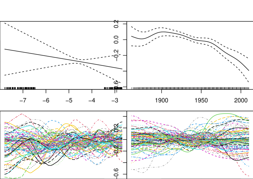
Figure 7:

Figure 8 provides a compelling visual representation of the model’s performance in capturing the complex relationship between log ASDRs and the mortality covariate $k_{t}$). The most striking aspect of this figure is the remarkable agreement between the fitted values and the observed values of log ASDRs. The closeness of the fitted values to the observed values illustrates the model’s ability to capture the underlying patterns in the data accurately. The figure clearly exhibits nonlinearity in the relationship between log ASDRs and $k_{t}$. Unlike a simple linear model, which may have struggled to capture this nonlinearity, the GAMM approach excels in accommodating and modeling the intricate non-linear patterns. The curves and deviations in the plot showcase the richness and complexity of the relationship. The figure serves as a compelling justification for employing the GAMM methodology. The pronounced nonlinearity in the data is vividly captured by the model, highlighting the necessity of using a flexible approach like GAMM. A simpler linear model would have likely fallen short in capturing these intricate patterns. The figure further reveals that the relationship between log ASDRs and $k_{t}$ differs across gender and between the two countries in the study. The separate curves for each gender and country underline the importance of accounting for these interactions and variations in the model. The agreement between fitted and observed values is not just visual; it is also statistically supported. This figure reinforces the strong statistical significance of the GAMM terms related to $k_{t}$ and the associated non-linear relationships. Therefore, this figure demonstrates the power of the GAMM approach in modelling and capturing the nonlinearity in the relationship between log ASDRs and the mortality covariate $k_{t}$. The close alignment between fitted and observed values affirms the model’s accuracy, while the presence of nonlinearity emphasizes the need for flexible modeling techniques like GAMM in complex data analysis.

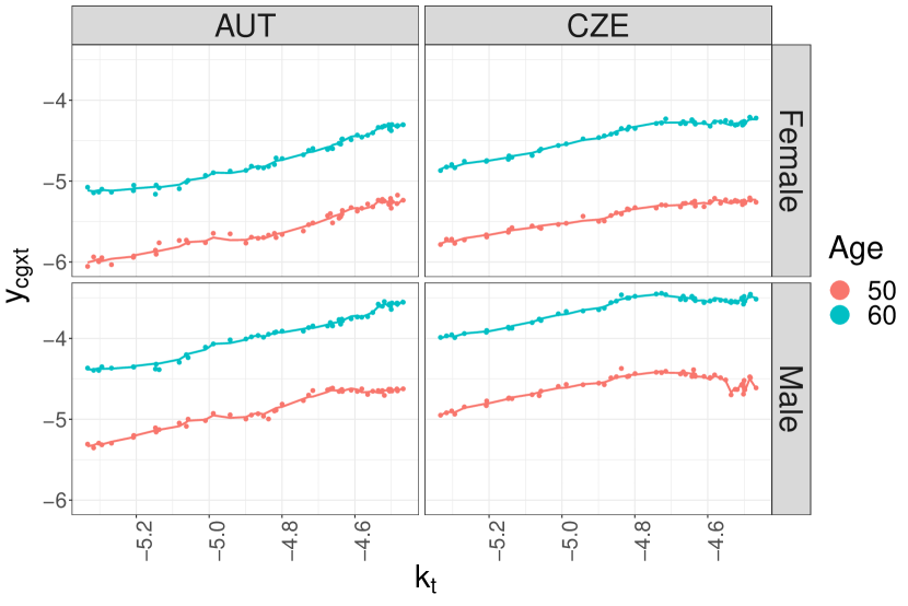
Figure 8: GAMM fits: $y_{cgxt}$ versus $k_{t}$. This plot highlights the GAMM’s ability to effectively capture nonlinear patterns, which the DK-LME model struggles to model accurately. It showcases how the GAMM approach excels in modelling and forecasting mortality rates, providing valuable insights into mortality dynamics.

Table 1 presents a comparison of Mean Square Error (MSE) between two models, the GAMM and the Li-Lee (LL) model, for forecasting mortality in four different populations. Notably, the findings reveal that the GAMM outperforms the LL model in forecasting accuracy for three out of four populations. These results underscore the significance of the GAMM’s effectiveness in providing more accurate mortality forecasts. The superior performance of the GAMM suggests that it may capture nuanced patterns and complexities in the data that the well-known LL model (Li and Lee 2005) does not account for, resulting in more precise predictions. These findings may have practical implications in various domains, including healthcare and policy-making, where accurate mortality forecasts are crucial. The ability of the GAMM to outperform the LL model in a majority of populations underscores the value of utilizing advanced modeling techniques to capture and leverage the intricacies of the data.

	AUT		CZE
Error	Female	Male	Female	Male
LL test set	$5.939*10^{-4}$	$7.058*10^{-4}$	$7.381*10^{-4}$	$2.354*10^{-3}$
GAM test set	$5.500*10^{-5}$	$7.386*10^{-4}$	$7.924*10^{-5}$	$7.816*10^{-4}$
LL test set/GAM test set	10.797	0.956	9.315	3.011

Table 1: MSE comparison between the GAM and LL models.

3 Modelling ASDRs in a Single Population

Our objective is to independently apply a population-specific variant of the GAMM, excluding cohort effects, to each distinct population as follows:

⬇

1model = bam(y $\sim$ age+s(kt,age,bs="fs",m=1),

2 data=ASDRs)

Listing 2: A GAMM for ASDRs in a single population.

4 Conclusion

References

- Antonio and Beirlant (2007) Antonio, K. and J. Beirlant (2007). Actuarial statistics with generalized linear mixed models. Insurance: Mathematics and Economics 40(1), 58–76.
- Frees et al. (2004) Frees, E. W. et al. (2004). Longitudinal and Panel Data: Analysis and Applications in the Social Sciences. Cambridge University Press.
- Hall and Friel (2011) Hall, M. and N. Friel (2011). Mortality projections using generalized additive models with applications to annuity values for the irish population. Annals of Actuarial Science 5(1), 19–32.
- Hastie (2017) Hastie, T. J. (2017). Generalized additive models. In Statistical models in S, pp. 249–307. Routledge.
- Hastie and Tibshirani (1986) Hastie, T. J. and R. J. Tibshirani (1986). Generalized additive models. Statistical Science Vol. 1(No. 3), 297–310.
- Hilton et al. (2019) Hilton, J., E. Dodd, J. J. Forster, and P. W. Smith (2019). Projecting uk mortality by using bayesian generalized additive models. Journal of the Royal Statistical Society Series C: Applied Statistics 68(1), 29–49.
- HMD (2023) HMD (2023). Human Mortality Database. University of California; Berkeley (USA); and Max Planck Institute for Demographic Research (Germany). Available at www.mortality.org or www.humanmortality.de (data downloaded on 05-20-2023].
- Li and Lee (2005) Li, N. and R. Lee (2005). Coherent mortality forecasts for a group of populations: An extension of the lee-carter method. Demography 42, 575–594.
- Plat (2009) Plat, R. (2009). On stochastic mortality modeling. Insurance: Mathematics and Economics 45(3), 393–404.
- (10) Wood, S. and M. S. Wood. Package ‘mgcv’.
- Wood (2003) Wood, S. N. (2003). Thin plate regression splines. Journal of the Royal Statistical Society Series B: Statistical Methodology 65(1), 95–114.
- Wood (2017) Wood, S. N. (2017). Generalized additive models: an introduction with R. CRC press.
- Wood et al. (2015) Wood, S. N., Y. Goude, and S. Shaw (2015). Generalized additive models for large data sets. Journal of the Royal Statistical Society Series C: Applied Statistics 64(1), 139–155.