Electronic Phase Propagation Speed in BaFe₂As₂ Revealed by Dilatometry

Abstract

Thermal expansion offers deep insights into phase transitions in condensed matter physics. Utilizing an advanced AC-temperature dilatometer with picometer resolution, this study clearly resolves the antiferromagnetic and structural transition in BaFe₂As₂. The implementation of temperature oscillation reveals a hysteresis near the transition temperature $T_{\mathrm{N}}$ with unprecedented resolution. Unexpectedly, we find that the hysteretic width exhibits a universal dependence on the parameters of temperature oscillation and the sample’s longidutinal dimension, which in turn reveals a finite transition speed. Our quantitative analysis shows that this phase boundary propagates at a mere 188 $\mu$m/s – a speed seven orders of magnitude slower than acoustic waves. This finding suggests a hidden thermodynamic constraint imposed by the electronic degrees of freedom.Our research not only sheds light on the dynamics of phase transitions between different correlated phases, but also establishes high precision dilatometry as a powerful tool for material studies. This measurement technique, when properly modified, can be extended to studies of other material properties such as piezoelectric, magneto-restriction, elastic modulus, etc.

I INTRODUCTION

Phase transitions are of great interest in the study of materials, where a variety of degrees of freedom are often coupled together. It is important to experimentally differentiate closely related transitions, as well as to identify the primary driving force behind a given transition. Because density is a true scalar that remains invariant under all symmetry operations relevant to solids, it is expected to have symmetry-allowed coupling to all phase transitions. As a result, accurately measured density can be used for detection (and classification) of phase transitions. In practice, this is often done with length measurements such as the linear thermal expansion coefficient $\alpha$[1, 2, 3, 4, 5, 6]. Along with atomic microscope piezocantilever, strain gauge, piezobender and X-ray diffraction[7, 8, 9, 10], the mostly used and accurate dilatometer is based on a plate capacitor. The length change of the sample $\Delta L$ is captured through monitoring the capacitance between the sample’s upper surface and a metal reference surface, and $\alpha$ is deduced by numerical differentiation $\alpha=L^{-1}{dL}/{dT}$ [11, 12, 13, 14, 15, 16]. Unfortunately, the sample is always at equilibrium, because this method needs an ultra-high temperature uniformity of the whole mechanichal structure to achieving its high accuracy, and its capacitance measurement limits temperature varying speed to $\sim 10^{-3}$ K/s.

In condensed matter physics, the dynamic behavior of phase transitions is always attractive and many techniques have been implemented [17, 18, 19, 20, 21]. Limited either by resolution or slow response, conventional dilatometers are not capable in studying the dynamic procedure of phase transitions. In this work, we present a new approach of measuring thermal expansion with pm-resolution using optical interferometers. Using oscillating temperature, we can analyze the dynamic response of the thermal expansion in the frequency domain. As a demonstration, we examine the anti-ferromagnetism phase transitions in BaFe₂As₂ [22, 23, 24, 25]. Our systematic investigation reveals a hysteresis that origins from the nonequilibrium state of sample near the transition temperature $T_{\mathrm{N}}$. The width of the hysteresis in temperature is proportional to the sample thickness $L$, the frequency and amplitude of temperature oscillation $\delta T$. Thanks to the continuous perturbation by $\delta T$, this hysteresis is likely a manifestation of the fact that the phase transitions is not infinitely sharp in time and the phase boundary propagates with a finite speed. The measured speed $\simeq 188$ $\mu$m/s is significantly smaller than the acoustic velocity, shining light on the complex nature of domain boundary dynamics.

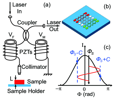
Figure 1: (a) Our dilatometer implements a fiber Michelson interferometer. The probing (left) and reference (right) arms are winded around cylindric PZT rings by which we can tune their length using the modulation and feedback voltages $V_{M}$ and $V_{F}$. $V_{M}$ generate a phase modulation $\phi_{M}=C\cos(\omega_{M}t)$, and $V_{F}$ eliminates the thermal drift $\Phi_{0}\approx 0$. (b) A detailed cartoon of the sapphire sample holder. The white, red and green meadow Pt wires are used as thermometer, AC and DC heaters. (c) The interfered light intensity $I=\cos(\Phi)$ is an odd function of the two beams’ phase difference $\Phi=\Phi_{M}+\phi_{S}$, where $\phi_{S}$ origins from the thermal expansion induced by the AC temperature oscillation. $\Phi$ oscillates between $\phi_{S}\pm C$ and the optical power difference between the two $\Phi$ extremes has a positive dependence on $\phi_{S}$; see text for detailed description of our measurement principle.

II EXPERIMENTAL SETUP

We use BaFe₂As₂, the parent compound of the “122” Fe-based superconductors, an ideal prototypical example of phase transition(s) with coupled degrees of freedom, for demonstration. It is generally believed to have a two-step phase transition when temperature reduces [22, 23, 24, 25], i.e. a second-order structural transition at $T_{\mathrm{S}}=134.5$ K followed by a first-order magnetic transition at $T_{\mathrm{N}}=133.75$ K [26, 27]. An electronic nematic phase is reported between $T_{\mathrm{S}}$ and $T_{\mathrm{N}}$ [28, 29, 30, 31, 32]. We study four samples (S1 to S4) with different thickness $L=$430, 210, 400 and 75 $\mu$m, respectively. Sample S1 and S2 are cleaved from the same piece, while S3 and S4 come from another one.

The sample is mounted on a sapphire sample holder which has three pairs of evaporated Pt wires used as thermometer, AC and DC heaters, respectively; see Fig. 1(b). We measure the thermometer resistance and calibrate it by the cryostat temperature when the heaters are switched off. The real-time sample temperature can be separated into a slowly sweeping DC part $T_{\mathrm{0}}$ by DC heater and an AC oscillation $\delta T$ by AC heater. $\delta T$ of sample induces an oscillation $\delta L$ in sample thickness and then the thermal expansion coefficient $\alpha$ can be deduced by $\alpha=L^{-1}\delta L/\delta T$ with the measurements of $\delta L$ and $\delta T$ by lock-in technique. We are able to achieve peformance comparable to the best reported capacitive dilatometry[16], i.e. pm-resolution in $\delta L$ amplitude $\langle\delta L\rangle$ and mK-resolution in $\delta T$ amplitude $\langle\delta T\rangle$, with dynamics measurement nature.

The $\delta L$ measurement of our dilatometer is based on a high resolution optical fiber Michelson interferometer and the output interference light intensity $I$ depends on the phase difference $\Phi$ between the probing and reference light beam as $I=I_{0}[1+\cos(\Phi)]$. We can tune the optical length of the two beams by applying the modulation and feedback voltages, $V_{M}$ and $V_{F}$, to the corresponding PZT rings; see Fig. 1(a). $\Phi$ consists three different components: the modulation phase $\phi_{M}=C\cos(2\pi f_{M}t)\propto V_{M}$, the AC phase signal $\phi_{S}=4\pi/\lambda\cdot\delta L$ where $\delta L=\alpha L\delta T$ is the sample’s thermal expansion induced by AC temperature oscillation $\delta T$, and the slowly varying $\phi_{0}$ caused by the thermal drift. $C$ and $f_{M}$ are the amplitude and frequency of the modulation, $\alpha$ is the thermal expansion coefficient and $\lambda=1550$ nm is the optical wavelength. We compensate the thermal drift using the feedback voltage $V_{F}$ so that $\phi_{0}$ can be neglected. According to the Jacobi-Anger expansion, the amplitudes of the output optical power’s $1^{\text{st}}$ and $2^{\text{nd}}$ harmonic component at $f_{M}$ and $2f_{M}$ are $I_{1}=I_{0}J_{1}(C)\sin(\phi_{S}(t))$ and $I_{2}=I_{0}J_{2}(C)\cos(\phi_{S}(t))$, respectively; $J_{N}$ is Bessel function of the $N$-th order. We measure $I_{1}\&I_{2}$ using lock-in technique to deduce the sample’s thermal expansion through

$$\delta L=\frac{\lambda}{4\pi}\tan^{-1}(\frac{J_{2}(C)I_{1}}{J_{1}(C)I_{2}})\approx\frac{J_{2}(C)\lambda}{4\pi J_{1}(C)I_{2}}\cdot I_{1}$$

The phase modulation frequency $f_{M}$ is typically a few kHz, the AC temperature oscillation frequency $f_{S}$ is 100 and 250 mHz, the feedback eliminates drifts at $\lesssim$ 0.1 Hz, and the $T_{\mathrm{0}}$ sweeping rate is $10^{-4}$ K/s. Our resolution of $\langle\delta L\rangle$ is as small as about 5 pm when using 50 mHz resolution bandwidth, so that we can use $\langle\delta T\rangle$ as small as 5 mK, see Fig. 3. You can find more detials about the design, principle and peformance of our dilatometer in Ref. [33] if you’re interested.

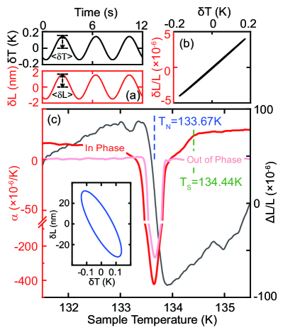
Figure 2: (a) The typical $\delta L$ and $\delta T$ oscillations measured at $T_{\mathrm{0}}\simeq 130$ K. (b) The $\delta L/L$ vs. $\delta T$ plot of panel (a) data. (c) The in-phase (red) and out-of-phase (pink) thermal expansion coefficient $\alpha$ by comparing $\delta L$ and $\delta T$ oscillations. The DC thickness variation $\Delta L$ (black) is deduced by $G\cdot V_{F}$. Data measured from sample S1 using $\delta T$ frequency $f_{S}=250$ mHz and amplitude $\langle\delta T\rangle=0.14$ K. The magnetic transition temperature $T_{\mathrm{N}}$ and structural transition temperature $T_{\mathrm{S}}$ are marked by blue and green dash lines, respectively. The inset illustrates the $\delta L$ vs. $\delta T$ hysteresis loop at $T=T_{\mathrm{N}}$.

III EXPERIMENTAL RESULTS

Fig. 2(a) shows typically measured $\delta T$ and $\delta L$ oscillations ($T_{\mathrm{0}}\simeq 130$ K). The phase of these two oscillations are perfectly aligned, leading to a linear line in Fig. 2(b) whose slope is the thermal expansion coefficient $\alpha$. $\alpha$ can be measured using lock-in technique by separating $\delta L$ oscillation into in-phase and out-of-phase components in reference to $\delta T$. The in-phase component of $\alpha$ is finite and its out-of-phase component remains nearly zero at temperatures away from $T_{\mathrm{N}}$, i.e. $T>134.5$ K or $T<133$ K, suggesting that the sample is at equilibrium and have uniform phase. Besides the AC differential measurement of $\alpha$, we can also measure the sample’s DC thickness change directly from the feedback voltage $V_{F}$ through $\Delta L=GV_{F}$, where $G=|{\lambda}/{\pi}\cdot{d\Phi}/{dV_{F}}|$ is the feedback gain.

In Fig. 2(c), $\Delta L$ taken from sample S1 ($L\simeq 430\mu$m) exhibits a jump of about $\Delta L/L\simeq 1\times 10^{-4}$ at $T_{\mathrm{N}}=133.67$ K where the in-phase component of $\alpha$ has a huge negative peak. This first-order phase transition is consistent with previous reports that the sample makes a transition from a high-temperature PM phase to a low-temperature AFM phase [26]. Unlike the smooth and gradual increase on the low temperature side of $T_{\mathrm{N}}$, $\alpha$ exhibit a clear kink in Fig. 2(c) at $T_{\mathrm{S}}\simeq 134.44$ K, signaling the second order phase transition. This is consistent with the work by M. G. Kim et al. where a structural transition from tetragonal to orthorhombic lattice is observed by high resolution X-ray diffraction studies [26].

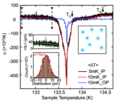
Figure 3: $\alpha$ measured using extremely small $\langle\delta T\rangle=$5mK and 10mK at 250 mHz from S2 (IP and OP are in-phase and out-of-phase part of $\alpha$, respectively). The abrupt $\alpha$ drop at $T_{\mathrm{O}}\simeq T_{\mathrm{N}}+0.1$ K suggests the formation of the AFM domains (blue dots) in the PM bath, illustrated by the right inset cartoon. The black dots represent the condensation nuclei of AFM domains, which might be defects. The left inset shows the measured $\langle\delta L\rangle$ in the range marked by the two vertical bars using 50 mHz resolution bandwidth. We deduce 5 pm resolution from the histogram of $\langle\delta L\rangle$ noise by subtracting the fitted green curve.

The small $\langle\delta T\rangle$ provides high resolution in temperature and reveals many features near the phase transition. Fig. 3 shows $\alpha$ measured from sample S2 ($L\simeq 210\mu$m) where $\langle\delta T\rangle$ is as small as 5 and 10 mK. The $\alpha$ peak of the S2 data is narrow and deep, evidencing its high quality since most of its bulk have the same $T_{\mathrm{N}}$. The temperature resolutions are about 10mK and 20mK and both of them are smaller than the detialed features of the $\alpha$ peak. Clear kinks in $\alpha$ appear at a temperature $T_{\mathrm{S}}$ about 0.8 K above $T_{\mathrm{N}}$, similar to sample S1, evidencing a strong link between these two transitions. Besides, we notice an extra abrupt change of $\alpha$ at $T_{O}\simeq T_{\mathrm{N}}+0.1$ K, which can be qualitative explained by the formation of AFM clusters around condensation nuclei such as defects while the substantial part of the sample remains PM, see the Fig. 3 inset [31].

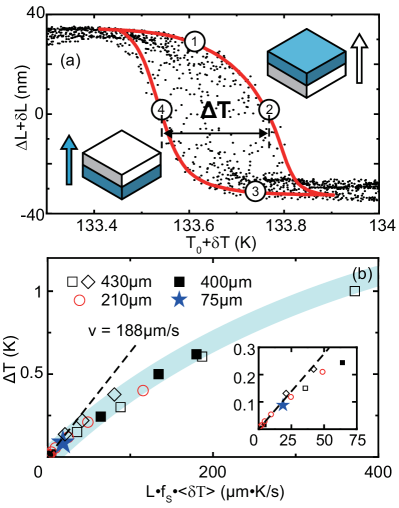
Figure 4: (a) The thickness-temperature hysteresis. Data measured using $f_{S}=100$ mHz and $\langle\delta T\rangle=0.25$ K. Note that the peak-to-peak amplitude of temperature oscillation is $2\langle\delta T\rangle=0.5$ K. We highlight one thermal cycle with thick red line and mark four positions in the loop. The inset cartoons illustrate the coexistence of the PM (white) and AFM (blue) phases and the propagation of their phase boundary. (b) Summarized $\Delta T$ vs. $Lf_{S}\langle\delta T\rangle$ measured from different samples. We use $f_{S}=100$ (open diamond) and 250 mHz (open square) for sample S1 data, and $f_{S}=250$ mHz for all other data. The uncertainty of is comparable to the symbol size. The inset is a zoon-in plot near zero.

Interestingly, the phase of $\delta L$ and $\delta T$ oscillation is no longer aligned near $T_{\mathrm{N}}$, signaled by the large out-of-phase component of $\alpha$ in Fig 2 and Fig 3. In another word, $\delta L$ vs. $\delta T$ exhibits a hysteric ellipse, as shown Fig. 2(c) inset. We choose the data of sample S1 at $f_{S}$=100 mHz and $\langle\delta T\rangle\simeq 0.25$ K as an example and sum the DC component $\Delta L$, induced by DC temperature $T_{\mathrm{0}}$ sweeping and measured by $V_{F}$, and the AC component $\delta L$, induced by AC temperature change $\delta T$ and measured by lock-in technique, as the real-time thickness of sample $\Delta L+\delta L$ and plot it as a function of the real-time temperature $T_{\mathrm{0}}+\delta T$ with black dots in Fig. 4(a). We hightlight the relationship between $\Delta L+\delta L$ and $T_{\mathrm{0}}+\delta T$ within the one period of $\delta T$ at $T_{\mathrm{0}}=T_{\mathrm{N}}$ with red line and all the real-time thickness dots at phase transition region fall inside the area enclosed by this red line. The clear square hysteresis loop indicates that the sample is off-equilibrium and has two coexisting phases at the transition.

A detailed and accurate description of this hysteresis involves the dynamic process of the phase transition which is rather complicated and beyond the scope of this article. Fortunately, we can understand the observed phenomenon using a simple toy model. In Fig. 4(a) we highlight one thermal loop with red line and the four numbers mark four different conditions. The sample starts from a uniform AFM phase at low temperature. When the temperature increases through $T_{\mathrm{N}}$ at spot 1, the PM phase appears at the sample’s bottom surface which is thermally anchored to the sample holder. The PM domain grows and the phase boundary propagates upward until it reaches the samples’ top surface. When we cool the sample back through $T_{\mathrm{N}}$ at spot 3, the AFM phase forms at the sample bottom and grows upward. We can identify two specific positions labeled 2 and 4 in Fig. 4(a), which correspond to the midway of the phase transition. At these two points, the sample is divided half-and-half into AFM and PM phases, see the inset cartoons. We define the distance between the two points, $\Delta T\simeq 0.22$ K, as the width of the hysteresis loop.

It is worthwhile to mention several facts about $\Delta T$. Firstly, the hysteresis width is not limited by the range of temperature oscillation, i.e. its the peak-to-peak amplitude $2\langle\delta T\rangle$. For example, $\Delta T\simeq 0.22$ K in Fig. 4(a) is about 40% of $2\langle\delta T\rangle\simeq 0.5$ K. This ratio becomes even smaller with slower frequency or thinner sample. Secondly, in contrast with systems such as supercooled pristine water which has liquid configuration well below its crystallization temperature if cooled slowly [34], the finite-width hysteresis loop is only because the temperature is changing “too fast” for this phase transition. $\Delta T$ vanishes when the amplitude or the frequency of $\delta T$ approaches zero. The ratio of out-of-phase part and in-phase part of $\alpha$ can symbolize $\Delta T$ qualitatively. So the extremely narrow peak of out-of-phase part of $\alpha$ at $\langle\delta T\rangle$ =10 mK showed in Fig. 3 comparing the width peak at $\langle\delta T\rangle$ =0.14 K showed in Fig. 2(c) also indicates the transition becomes infinitely sharp if we sweep the AC temperature change sufficiently slow, which is consistent with previous capacitive dilatometry studies where no hysteresis is seen.

We measure the hysteresis loop from different samples using different $\delta T$ frequencies $f_{S}$ and amplitudes $\langle\delta T\rangle$. We use $f_{S}=100$ and 250 mHz to measure S1, and $f_{S}=250$ mHz for the other samples. We find that $\Delta T$ is proportional to the sample thickness $L$, the AC temperature oscillation frequency $f_{S}$ and amplitude $\langle\delta T\rangle$. We summarize $\Delta T$ as a function of $L\cdot f_{S}\langle\delta T\rangle$ in Fig. 4(b). It is quite remarkable that all data points collapse onto the same curve highlighted by the blue band. We note that the phase boundary propagates by a distance $L/2$ to the midway of the sample from its bottom surface at spots 2 and 4 as shown in the cartoons of Fig. 4(a), and $f_{S}\langle\delta T\rangle$ is the maximum temperature changing rate. Therefore, the slope of the blue curve corresponds to the propagation speed of phase boundary which is $v=188$ $\mu$m/s at small $L\cdot f_{S}\langle\delta T\rangle$. This speed is seven orders of magnitude lower than that of acoustic waves [35]. The constraint on the phase boundary propagation speed is likely related to magnetoelastic nature of the transition at $T_{\mathrm{N}}$ where the electronic degrees of freedom correlates with the lattice deformation.

IV CONCLUSION

Our study of thermal expansion coefficient of BaFe₂As₂ using an interferometer-based dilatometer reveals interesting information of its magnetic transition. Our results clearly resolve the two-step transition where the second-order structural transition appears at $T_{\mathrm{S}}$ and the first-order magnetic transition at $T_{\mathrm{N}}$. Thanks to the extremely high resolution and the ”true” differential nature of our technique, we discover the samples’ thickness-temperature hysteresis loop at $T_{\mathrm{N}}$. We can describe this dynamic process with a simple model and our systematical study reveals a propagation speed of phase boundary to be $v=188$ $\mu$m/s. This work highlights that AC-temperature dilatometry with extraordinarily high resolution is a powerful probe of correlation effects in quantum materials and it’s a completely new high resolution approach for phase transition research. This measurement technique can also be extended to studies of other material properties such as piezoelectric, magneto-restriction, elastic modulus, etc with proper modification.