Asymptotic stability and cut-off phenomenon for the underdamped Langevin dynamics

Abstract.

In this article, we provide detailed analysis of the long-time behavior of the underdamped Langevin dynamics. We first provide a necessary condition guaranteeing that the zero-noise dynamical system converges to its unique attractor. We also observed that this condition is sharp for a large class of linear models. We then prove the so-called cut-off phenomenon in the small-noise regime under this condition. This result provides the precise asymptotics of the mixing time of the process and of the distance between the distribution of the process and its stationary measure. The main difficulty of this work relies on the degeneracy of its infinitesimal generator which is not elliptic, thus requiring a new set of methods.

1. Introduction

1.1. Underdamped Langevin dynamics

We start by introducing the underdamped Langevin dynamics which are the main concern of the current article. In statistical physics the evolution of a molecular system at a fixed temperature $T$ consisting of $N$ particles can be modeled by the underdamped Langevin dynamics $(q_{t},\,p_{t})\in\mathbb{R}^{d}\times\mathbb{R}^{d}$, $d=3N$, where $q_{t}\in\mathbb{R}^{d}$ and $p_{t}\in\mathbb{R}^{d}$ denote the vectors of positions and momenta of the particles. The process $(q_{t},\,p_{t})$ satisfies a system of stochastic differential equations of the form

$$\left\{\begin{aligned} &\mathrm{d}q_{t}=M^{-1}p_{t}\mathrm{d}t,\\ &\mathrm{d}p_{t}=F(q_{t})\mathrm{d}t-\gamma M^{-1}p_{t}\mathrm{d}t+\sqrt{2\gamma\beta^{-1}}\mathrm{d}B_{t}\;,\end{aligned}\right.$$ (1.1)

where $M\in\mathbb{R}^{d\times d}$ is the mass matrix, $F:\mathbb{R}^{d}\to\mathbb{R}^{d}$ is the force acting on the particles, $\gamma>0$ is the friction parameter, and $\beta^{-1}=k_{B}T$ with $k_{B}$ the Boltzmann constant and $T$ the temperature of the system. Such dynamics can be used to compute thermodynamic quantities of the process.

Thermodynamic quantities are averages of given observables against the stationary distribution of (1.1). They capture the characteristics of the system at equilibrium and offer numerous applications in biology, chemistry and materials science. However, the computation of such quantities poses a certain number of computational challenges. In fact, direct numerical integration is in general very difficult when the number of particles $N$ is large and thus the space dimension when computing integrals against the stationary distribution. This is why stochastic approaches are generally preferred and consist in computing the time-average of the observable. Using the ergodicity of (1.1), such time averages shall converge to the expected thermodynamic limit. However, the speed of convergence relies heavily on how fast the process (1.1) converges to its stationary distribution. Therefore, one area of research is to understand the dependency of this speed of convergence to equilibrium in the low temperature regime, i.e. $\beta^{-1}$ goes to $0$. In the current article, we completely solve this problem by verifying the so-called the cut-off phenomenon for the underdamped Langevin processes under a suitable reasonable condition on the vector field $F$.

Main results of the article

To be more precise, we set $M=\mathbb{I}_{d}$ and $\epsilon=\gamma k_{B}T>0$ so that we can rewrite (1.1) as

$$\begin{cases}\mathrm{d}q_{t}^{\epsilon}=p_{t}^{\epsilon}\mathrm{d}t,\\ \mathrm{d}p_{t}^{\epsilon}=-F(q_{t}^{\epsilon})\mathrm{d}t-\gamma p_{t}^{\epsilon}\mathrm{d}t+\sqrt{2\epsilon}\mathrm{d}B_{t}\;,\end{cases}$$ (1.2)

Then, we are interested in the behavior of the $2d$-dimensional process $X_{t}^{\epsilon}=(q_{t}^{\epsilon},\,p_{t}^{\epsilon})$ in the low-temperature regime, i.e., the regime where $\epsilon$ tends to $0$. We first provide the necessary condition (cf. Assumption 2.2) to the vector field $F$ under which the zero-temperature dynamics, i.e., the dynamics (1.2) with $\epsilon=0$ converges, as $t\rightarrow\infty,$ to a unique stable equilibria of the dynamics. As we can observe from the discussion below, this condition is very close to the necessary and sufficient condition in the sense that for the large-class of linear model our condition is indeed necessary and sufficient.

Under this condition, we demonstrate in Proposition 2.6 that the process $(X_{t}^{\epsilon})_{t\geq 0}$ is positive recurrent and therefore admits a unique stationary probability measure $\mu_{\epsilon}$. Then, by the standard erodicity argument, the distribution of the process $(X_{t}^{\epsilon})_{t\geq 0}$, starting from any fixed point in $\mathbb{R}^{d}\times\mathbb{R}^{d}$, converges to $\mu_{\epsilon}$, as $t\rightarrow\infty$ (thermalization). The precise quantitative analysis of this convergence is the main problem confronted in the current article. In fact, we prove the so-called cut-off phenomenon which will be explained in the next subsection.

1.2. Cut-off phenomenon

The convergence to equilibrium for stochastic diffusion processes sometimes exhibits a brutal decrease around a cut-off time where the total-variation distance between the law of the process and its equilibrium goes from a value close to $1$ to a value close to $0$. This fact is known as cut-off phenomenon.

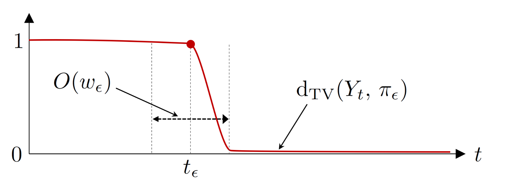
Figure 1.1. Illustration of the cut-off phenomenon: the red line is the graph of the function $d(t)=\textrm{d}_{\textrm{TV}}(Y_{t}^{\epsilon},\,\pi_{\epsilon})$ which abruptly drops from values close to $1$ to values close to $0$ at $t=t_{\epsilon}$ in the window of size $w_{\epsilon}$

Definition 1.1 (Cut-off phenomenon).

For $\epsilon>0$, let $(Y_{t}^{\epsilon})_{t\geq 0}$ be a Markov process with stationary probability measure $\pi_{\epsilon}$. We denote by $\mathrm{d}_{\mathrm{TV}}\left(\cdot,\,\cdot\right)$ the total-variation distance (for the precise definition, we refer to Definition 2.7) so that $\mathrm{d}_{\mathrm{TV}}\left(Y_{t}^{\epsilon},\,\pi_{\epsilon}\right)$ represents the total-variation distance between the distribution of $Y_{t}^{\epsilon}$ (for fixed time $t\geq 0$) and $\pi_{\epsilon}$. Then, we say that the process $(Y_{t}^{\epsilon})_{t\geq 0}$ exhibits the cut-off at mixing time $t^{\epsilon}$ with the window $w^{\epsilon}$ satisfying

$$\lim_{\epsilon\rightarrow 0}t^{\epsilon}=\infty\quad\text{and}\quad\lim_{\epsilon\rightarrow 0}\frac{w^{\epsilon}}{t^{\epsilon}}=0\;,$$

if we have

$$\begin{cases}\lim_{c\rightarrow+\infty}\limsup_{\epsilon\rightarrow 0}\mathrm{d}_{\mathrm{TV}}\left(Y_{t^{\epsilon}+cw^{\epsilon}}^{\epsilon},\,\pi_{\epsilon}\right)=0\;,\\ \lim_{c\rightarrow-\infty}\liminf_{\epsilon\rightarrow 0}\mathrm{d}_{\mathrm{TV}}\left(Y_{t^{\epsilon}+cw^{\epsilon}}^{\epsilon},\,\pi_{\epsilon}\right)=1\;.\end{cases}$$ (1.3)

We refer to Figure 1.1 for an illustration of the cut-off phenomenon. The cut-off phenomenon implies that, the distribution of the process $Y_{t}$ converges to its stationary measure abruptly at the mixing time $t_{\epsilon}$ within the window of size $w_{\epsilon}\ll t_{\epsilon}$.

Moreover, we say that there is profile cut-off or profile thermalisation with the profile $G:\mathbb{R}\rightarrow[0,\,1]$ which is a decreasing function with $G(-\infty)=1$ and $G(+\infty)=0$ if we have

$$\lim_{\epsilon\rightarrow 0}\mathrm{d}_{\mathrm{TV}}\left(Y_{t^{\epsilon}+cw^{\epsilon}}^{\epsilon},\,\pi_{\epsilon}\right)=G(c)$$ (1.4)

for all $c\in\mathbb{R}$. Of course, the profile cut-off is a stronger notion than cut-off since (1.4) immediately implies (1.3).

Remark 1.2.

Although we explain the cut-off phenomenon in the regime $\epsilon\rightarrow 0$ to match with the main result of the current article, the other models can exhibit the cut-off phenomenon in a different regime, e.g., $N\rightarrow\infty$ where $N$ is the number of sites in a spin system.

In the modern study of the mixing behavior of the statistical phyics systems, the cut-off phenomenon has been verified for various stochastic systems. For instance, the cut-off phenomenon has been widely verified for high-temperature spin systems such as the Glauber dynamics of the Curie-Weiss type mean-field model, [15, 3, 32], the Glauber dynamics of the Ising/Potts model on lattices [20, 21, 23, 22], the Swandsen-Wang dynamics of the Ising/Potts model [27], and the FK-dynamics of the random-cluster model [8]. The cut-off phenomenon is also widely observed in the interacting particle systems such as the zero-range processes [25], the exclusion processes [9, 5, 30], and the east process [7]. It is also demonstrated that the cut-off phenomenon is universally observed for the random walks on nicely expanding graphs, see [18, 19, 17]. We also refer to the monograph [16] for the introduction to this huge topic.

1.3. Cut-off phenomenon for underdamped Langevin dynamics

In [2], the cut-off phenomenon for the overdamped Langevin dynamics $(\overline{q}_{t}^{\epsilon})_{t\geq 0}$ in $\mathbb{R}^{d}$ defined by

$$\mathrm{d}\overline{q}_{t}^{\epsilon}=-F(\overline{q}_{t}^{\epsilon})\mathrm{d}t+\sqrt{2\epsilon}\mathrm{d}B_{t}\;,$$ (1.5)

where $F\in\mathcal{C}^{3}(\mathbb{R}^{d},\,\mathbb{R}^{d})$ and where $(B_{t})_{t\geq 0}$ denotes the $d$-dimensional Brownian motion has been established. In this work, it has been assumed that there exist constants $\delta,C,\eta>0$ such that for all $q,q^{\prime}\in\mathbb{R}^{d}$,

$$\langle q,\mathrm{D}F(q^{\prime})q\rangle\geq\delta|q|^{2}\;\;\;\text{and}\;\;\;|F(q)|\leq C\mathrm{e}^{\eta|q|^{2}}\;.$$ (1.6)

In particular, the first condition implies the coercivity of the process, i.e., there is a strong contracting property for the process $(\overline{q}_{t}^{\epsilon})_{t\geq 0}$ starting from different starting points. Under these conditions, the cut-off for the process $(\overline{q}_{t}^{\epsilon})_{t\geq 0}$ starting from any fixed point is proven in [2] where the mixing time is of order $\log\frac{1}{\epsilon}$ and the window is of order $1$. The mixing time is computed explicitly in [2, Lemma 2.1]. The authors also provide in [2, Corollary 2.9] a necessary and sufficient condition under which profile thermalisation holds.

Our main purpose in this work is to extend the existence of such cut-off phenomenon to the underdamped Langevin dynamics. Several difficulties appear when considering the underdamped Langevin dynamics. The first one concerns the asymptotic stability of the associated deterministic dynamics $(\epsilon=0)$ which is a crucial element of the proof in the overdamped case (1.5). In fact, to the best of our knowledge, when $F$ is not in gradient form (i.e., $F=\nabla V$ for some $V$), no criterion was available in the literature to ensure such stability. We can also show that the same condition appearing in the overdamped case (1.6) is not enough to ensure stability in the underdamped case. We are able however to provide in this work a sharp criterion on $F$ ensuring global stability. This criterion is even shown to be necessary and sufficient when $F(q)=\mathbb{M}q$ with $\mathbb{M}$ being a normal matrix (i.e. $\mathbb{M}\mathbb{M}^{\dagger}=\mathbb{M}^{\dagger}\mathbb{M}$).

In the proof of the cut-off, the main difficulty arises from the lack of the ellipticity of the underdamped Langevin dynamics, for which the diffusion matrix is not even invertible. Generally, this hypoellipticity causes multitude of fundamental difficulties in the study of the underdamped Langevin dynamics, and the current work also has to confront this difficulty.

In the proof of the cut-off for the overdamped Langevin dynamics, the solution $\Sigma$ to a matrix Lyapunov equation of the form

$$\textup{D}F(0)\Sigma+\Sigma\,\textup{D}F(0)^{\dagger}=\mathbb{I}_{d}$$ (1.7)

plays a significant role. However, in the underdamped case, the matrix in the right-hand side which comes from the diffusion matrix of the process is not invertible. Therefore, the standard result applied does not ensure the positive definiteness of the solution. We shall however prove such property by using the inherent dependency between position and velocity coordinates. Moreover, in the overdamped Langevin case, it is shown that the solution to the matrix Lyapunov equation (1.7) is the long-time limit of the covariance matrix of a Gaussian process used to approximate the overdamped process $(\overline{q}_{t}^{\epsilon})_{t\geq 0}$. As we shall see later, such proof is not applicable as it crucially uses the ellipticity of the process. Finally, one also needs to provide a control in $\epsilon$ of the tails of the stationary distribution $\mu^{\epsilon}$ for which there is not much literature when $F$ is not conservative.

All in all, such difficulties are fundamental and require deeper understanding of the underdamped Langevin dynamics which we provide in this work. Thus, we strongly believe these new results can be used in further work involving the underdamped Langevin dynamics.

2. Model and Main Results

2.1. Stability of underdamped Langevin dynamics

Zero-noise dynamics

In this article, we investigate the thermalisation of the underdamped Langevin dynamics $(X_{t}^{\epsilon})_{t\geq 0}=(q_{t}^{\epsilon},\,p_{t}^{\epsilon}){}_{t\geq 0}$ in $\mathbb{R}^{d}\times\mathbb{R}^{d}$ defined in (1.2). To that end, we first have to understand the behaviour of the associated zero-noise dynamics by setting $\epsilon=0$ in (1.2). More precisely, the zero-noise dynamics $(X_{t})_{t\geq 0}=(q_{t},\,p_{t})_{t\geq 0}$ then satisfies the following ordinary differential equation

$$\begin{cases}\mathrm{d}q_{t}=p_{t}\mathrm{d}t,\\ \mathrm{d}p_{t}=-F(q_{t})\mathrm{d}t-\gamma p_{t}\mathrm{d}t\;.\end{cases}$$ (2.1)

We assume here that $F(0)=0$ so that $(0,\,0)\in\mathbb{R}^{d}\times\mathbb{R}^{d}$ is an equilibrium point of the deterministic dynamics $(X_{t})_{t\geq 0}$. In particular, we are interested in the situation when the dynamics $(X_{t})_{t\geq 0}$ admits the unique stable equilibrium $(0,\,0)$. Additionally, we would like to ensure the global asymptotic stability of $(X_{t})_{t\geq 0}$ meaning that starting from any initial point $X_{0}=x\in\mathbb{R}^{2d}$,

$$\lim_{t\rightarrow\infty}X_{t}=(0,0)\in\mathbb{R}^{2d}\;.$$ (2.2)

We shall provide in this work a condition on the force $F$ ensuring the global exponential stability of the dynamical system $(X_{t})_{t\geq 0}$ meaning that there exist $\lambda,\,C>0$ such that starting from any point $X_{0}=x\in\mathbb{R}^{2d}$,

$$|X_{t}|^{2}\leq Ce^{-\lambda t}\;\;\;\text{for all\;}t\geq 0\;,$$ (2.3)

where $C$ is a constant depending on the starting location $x$, while $\lambda$ is a constant indepdent of $x$. Note that we cannot hope such a contraction for a dynamics of the form (2.1) since the time-derivative of $|X_{t}|^{2}$ is given by

$$\frac{\textup{d}}{\textup{d}t}|X_{t}|^{2}=2\left[q_{t}p_{t}+p_{t}(-F(q_{t})-\gamma p_{t})\right]$$ (2.4)

has no reason to be negative for all $(q_{t},p_{t})\in\mathbb{R}^{2d}$. In fact, as one can observe from an example of the flow diagram of $X_{t}$ given in Figure 1.1, the $L^{2}$-norm $|X_{t}|^{2}$ may increase at certain times $t_{0}$ since the trajectory of $X_{t}$ is an elliptical rotation around the stable equilibria. This feature makes the asymptotic stability analysis of $(X_{t})_{t\geq 0}$ a non-trivial question. In particular, previous studies such as [2] on the overdamped model (1.5) assumed $F$ to satisfy certain condition (cf. [2, condition (C)]) ensuring that the zero-noise dynamics satisfies

$$\frac{\textup{d}}{\textup{d}t}|X_{t}|^{2}\leq-\lambda|X_{t}|^{2}\;\;\;\text{for some }\lambda>0\;,$$ (2.5)

and thus global exponential stability. However, we notice from (2.4) that there is no condition on $F$ which could possibly ensure (2.5) for the underdamped Langevin dynamics as well.

We finally remark that, in the case where the dynamical system $(X_{t})_{t\geq 0}$ admits multiple stable equilibria, the underdamped Langevin dynamics $(X_{t}^{\epsilon})_{t\geq 0}$ exhibits metastability among these stable equilibria. This question was studied in an consecutive work [13] by the authors of the current article.

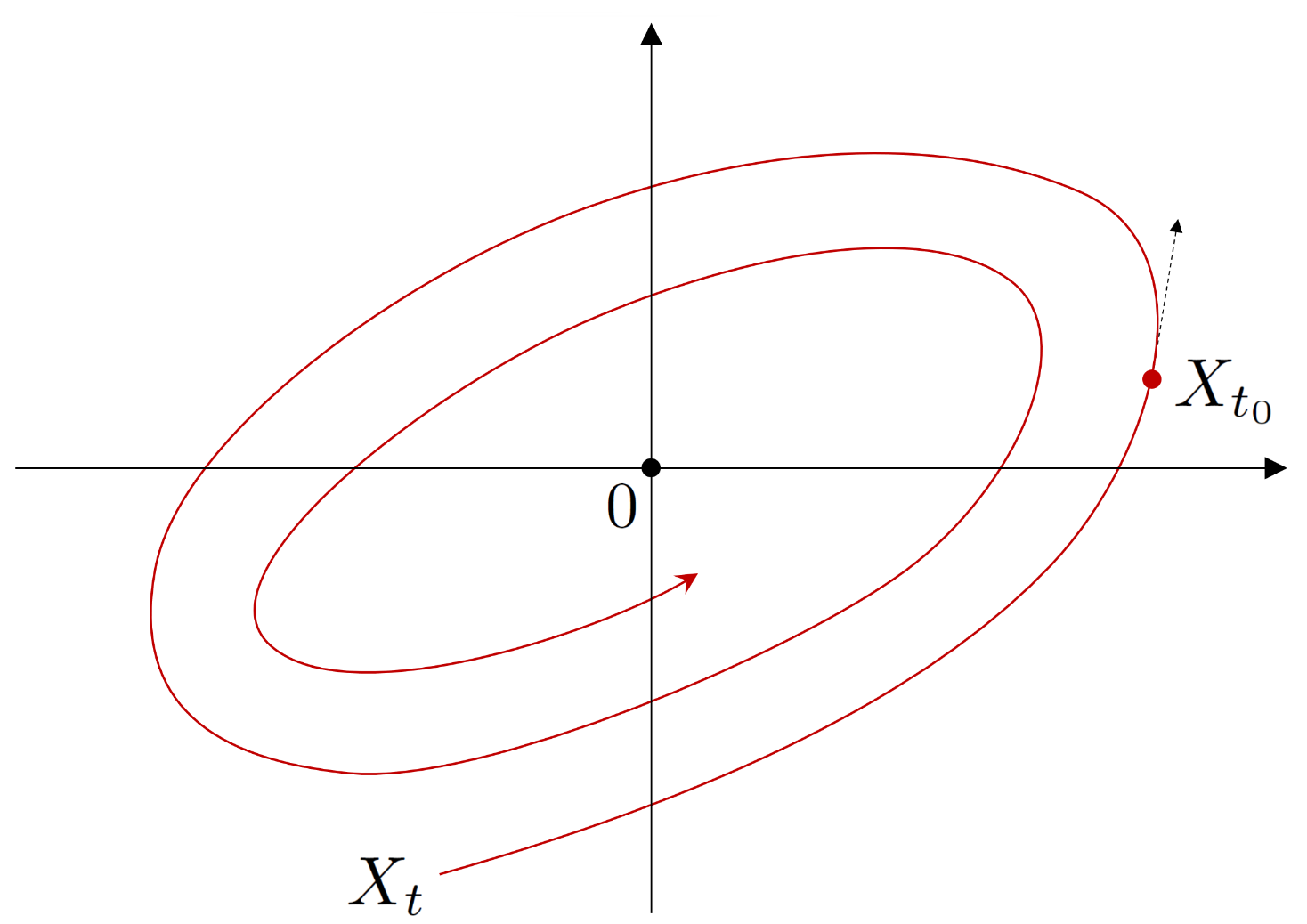
Figure 2.1. Trajectory of $(X_{t})_{t\geq 0}$: the $L^{2}$-norm $|X_{t}|^{2}$ may increase at certain time $t_{0}$ since the trajactory converges to the origin by elliptically rotating

Brief introduction to the main results

Our first main result provides a sufficient condition (Assumption 2.2) under which the zero-noise dynamical system $(X_{t})_{t\geq 0}$ is globally exponentially stable. This result is stated in Theorem 2.3 of Section 2.2. We believe that this is the first non-trivial criterion ensuring global asymptotic stability of the underdamped system $(X_{t})_{t\geq 0}$ when the vector field $F$ does not write as a gradient of a potential function. Furthermore, in the linear case when $F(q)=\mathbb{M}q$ for some constant matrix $\mathbb{M}$ we shall prove in Section 3.2 that our sufficient condition given in Assumption 2.2 is close to a necessary and sufficient condition.

In Section 2.3, we study the low-temperature behavior of the underdamped Langevin dynamics $(X_{t}^{\epsilon})_{t\geq 0}$, i.e. when $\epsilon$ is close to zero, under the exponential stability property obtained in Theorem 2.3. In particular, this allows us to obtain an asymptotic analysis of the invariant distribution of $(X_{t}^{\epsilon})_{t\geq 0}$ (Theorem 2.8) and the sharp characterization of the convergence of the distribution of $X_{t}^{\epsilon}$ towards its stationary measure when $t$ goes to infinity (Theorem 2.12). In particular, we verify the cut-off phenomenon for the underdamped Langevin dynamics.

Notation 2.1.

We shall use the following notation throughout this article.

1. We denote by $\mathbb{M}^{\dagger}$ (resp. $\mathbb{M}^{*}$) the transpose (resp. conjugate transpose) matrix of a square complex-valued matrix $\mathbb{M}$.

2. Any appearance of $x$ denotes an element of $\mathbb{R}^{2d}$. We shall denote implicity by $q\in\mathbb{R}^{d}$ its position vector and $p\in\mathbb{\mathbb{R}}^{d}$ its velocity vector such that $x=(q,\,p)$.

3. We denote by $X_{t}^{\epsilon}(x)=(q_{t}^{\epsilon}(x),\,p_{t}^{\epsilon}(x))$ (resp. $X_{t}(x)=(q_{t}(x),\,p_{t}(x))$) the process $(X_{t}^{\epsilon})_{t\geq 0}$ satisfying (1.2) (resp. $(X_{t})_{t\geq 0}$ satisfying 2.1) at time $t$ and starting from $x\in\mathbb{R}^{2d}$, i.e., $X_{0}^{\epsilon}(x)=x$ (resp. $X_{0}(x)=x$) almost-surely. We will not stress the starting point and merely write $X_{t}^{\epsilon}$ and $X_{t}$ when we do not need to emphasize the starting point.

2.2. Asymptotic stability analysis of zero-noise dynamics

To state our first main result, we introduce the following assumption on $F$ which guarantees the global exponential stability of $(X_{t})_{t\geq 0}$ (2.3).

Assumption 2.2.

The vector field $F\in\mathcal{C}^{3}(\mathbb{R}^{d},\mathbb{R}^{d})$ appearing in (1.2) and (2.1) can be decomposed into

$$F=\nabla U+\ell\;,$$ (2.6)

for some non-negative function $U\in\mathcal{C}^{4}(\mathbb{R}^{d},\mathbb{R})$ and vector field $\ell\in\mathcal{C}^{3}(\mathbb{R}^{d},\mathbb{R}^{d})$ satisfying, for some constants $\alpha\in(0,\,\infty)$, $\beta\in(0,\,\gamma)$,

$$\left\langle F(q),\,q\right\rangle\geq\alpha\left(|q|^{2}+U(q)\right)+\frac{|\ell(q)|^{2}}{\beta^{2}}\;\;\;\text{for all }q\in\mathbb{R}^{d}\;.$$ (2.7)

Under the assumption above, the following global exponential stability of the deterministic dynamics $(X_{t})_{t\geq 0}$ described by (2.1) can be stated.

Theorem 2.3.

Under Assumption 2.2, there exist constants $\kappa,\lambda>0$ independent of $x\in\mathbb{R}^{2d}$ such that (cf. Notation 2.1)

$$|X_{t}(x)|^{2}\leq\kappa\left[|x|^{2}+U(q)\right]\mathrm{e}^{-\lambda t}\;\;\;\text{for all }t\geq 0\;.$$ (2.8)

The proof of this theorem is based on the construction of a suitable Lyapunov function and shall be carried out in Section 4.

Remark 2.4.

The followings are explanations on Assumption 2.2 and Theorem 2.3.

1. Necessity of Assumption 2.2. In view of Theorem 2.5 below, Assumption 2.2 (which might seem to be technical at first glance) is in fact not only natural but also necessary in a large class of models to get global asymptotic stability in the sense of (2.2).

2. Meaning of condition 2.7. The condition (2.7) implies that $\ell$ should not be too large, and hence in view of (2.6), the force $F$ should be sufficiently close to a gradient force attracting towards the stable equilibrium. We note that, in the overdamped model, as explained in [2, condition (C) and display (2.2)], it suffices to have $F(q)\cdot q\geq\alpha|q|^{2}$ for all $q\in\mathbb{R}^{d}$ for some positive constant $\alpha$ in order to ensure global asymptotic stability. However, in the underdamped model, if $|\ell(q)|$ is too large so that the condition (2.7) is violated, then such stability fails as will be shown in Section 3.

3. Decomposition 2.6 in the overdamped model. The decomposition of the form (2.6) is standard, e.g. [6, 11, 12, 28] in the overdamped model. In this literature, it is also often assumed that this decomposition satisfies the orthogonality condition $\nabla U\cdot\ell\equiv 0$, which we did not need to assume in this work.

4. Equilibria of dynamical system $(X_{t})_{t\geq 0}$ under Assumption 2.2. Note first that, since adding a constant to $U$ does not change $\nabla U$ in (2.6), the non-negativity assumption on $U$ amounts to assuming that $U$ is bounded from below. Additionally, taking $q=0$ in (2.7), we obtain $U(0)=0$ and $\ell(0)=0$. The former implies that $0$ is a global minimum of $U$ (by the non-negativity assumption), and hence $\nabla U(0)=0$. Therefore $(0,0)$ is an equilibrium point of $(X_{t})_{t\geq 0}$. On the other hand, suppose that $x_{0}=(q_{0},\,p_{0})$ is an equilibrium point of the dynamics (2.1). we should have $p_{0}=F(q_{0})=0$. Inserting $q=q_{0}$ into (2.7), we get $|q_{0}|^{2}=0$ (since $U$ is non-negative) and thus $q_{0}=0$. Therefore, condition (2.7) implies that $(0,\,0)$ is the unique equilibrium point of the dynamics (2.1).

5. Quadratically growing $U$. When $U$ grows at most quadratically, i.e., there exists $C>0$ such that

   $$|U(q)|\leq C|q|^{2}\;\;\;\text{for all }q\in\mathbb{R}^{d}\;,$$ (2.9)

   we notice that the condition (2.7) is equivalent to the existence of $\alpha>0$ and $\beta\in(0,\gamma)$ such that

   $$\left\langle F(q),\,q\right\rangle\geq\alpha|q|^{2}+\frac{|\ell(q)|^{2}}{\beta^{2}}\;\;\;\text{for all }q\in\mathbb{R}^{d}\;,$$ (2.10)

   and moreover we can replace (2.8) by

   $$|X_{t}(x)|^{2}\leq\kappa|x|^{2}\mathrm{e}^{-\lambda t}\;\;\;\text{for all }t\geq 0\;.$$ (2.11)

6. Regularity assumption on $F$. Although we assumed that $F\in\mathcal{C}^{3}(\mathbb{R}^{d},\,\mathbb{R}^{d})$, a careful reading of the proof reveals that the conditions $F\in\mathcal{C}^{2}(\mathbb{R}^{d},\,\mathbb{R}^{d})$ and $F$ is $\mathcal{C}^{3}$ in a neighborhood of the origin are indeed sufficient. The regularity of $U$ and $\ell$ imposed in Assumption 2.2 can be weakened accordingly.

Linear model and necessity of Assumption 2.2

The theorem below ensures that Assumption 2.2 is a necessary and sufficient condition for a large class of linear forces $F$.

Theorem 2.5.

Suppose that $F(q)=\mathbb{M}q$ with $\mathbb{M}$ being a normal matrix, i.e. $\mathbb{M}\mathbb{M}^{\dagger}=\mathbb{M}^{\dagger}\mathbb{M}$. Then, the dynamics (2.1) is asymptotically stable if and only if $F$ satisfies Assumption 2.2.

The proof of this theorem will be given in Section 3. In particular, this theorem is a consequence of Theorem 3.4 which completely characterizes the necessary and sufficient condition on $\mathbb{M}$ under which the dynamics (2.1) is globally asymptotically stable. Notice that in the linear case global asymptotic stability is equivalent to asymptotic stability starting from any point.

2.3. Thermalization of underdamped Langevin dynamics

Let us assume that $F$ satisfies Assumption 2.2 so that the zero-noise dynamics exhibits the global exponential stability towards $0$ stated in our first result Theorem 2.3. We shall prove in Section 4.4 that the underdamped process $(X_{t}^{\epsilon})_{t\geq 0}$ admits in fact a unique stationary distribution $\mu^{\epsilon}$.

Proposition 2.6.

The process $(X_{t}^{\epsilon})_{t\geq 0}$ admits a unique stationary distribution $\mu^{\epsilon}$.

Our second result investigates the thermalization behavior of the process $(X_{t}^{\epsilon})_{t\geq 0}$ in the regime $\epsilon\rightarrow 0$ to its stationary measure $\mu_{\epsilon}$. Our concern is to describe in more detail the underlying cut-off phenomenon involved in this convergence when $\epsilon$ goes to zero.

This convergence is studied under the total variation distance defined below.

Definition 2.7 (Total variation distance).

For two probability measures $\pi_{1}$ and $\pi_{2}$ on $\mathbb{R}^{2d}$ (with the measure space consisting of Lebesgue measurable sets), we define the total variation distance between $\pi_{1}$ and $\pi_{2}$ as

$$\textup{d}_{\textup{TV}}(\pi_{1},\,\pi_{2})=\sup_{A}\left|\pi_{1}(A)-\pi_{2}(A)\right|\;,$$

where the supremum is taken over all Lebesgue measurable sets in $\mathbb{R}^{2d}$. When the law of a random vector $Z_{i}\in\mathbb{R}^{2d}$ is $\pi_{i}$ ($i=1,\,2)$, we can substitute $\pi_{i}$ above with $Z_{i}$. For instance, $\textup{d}_{\textup{TV}}(Z_{1},\,\pi_{2})$ and $\textup{d}_{\textup{TV}}(Z_{1},\,Z_{2})$ also represent $\textup{d}_{\textup{TV}}(\pi_{1},\,\pi_{2})$.

Stationary measure

An important difficulty arising in the study of $\textup{d}_{\textup{TV}}(X_{t}^{\epsilon},\,\mu_{\epsilon})$ is that the stationary measure $\mu^{\epsilon}$ cannot be given explicitly when the force $F$ does not write as a gradient function. However, for the purpose of this work, we are able to compute an asymptotic behavior of $\mu^{\epsilon}$ when $\epsilon$ goes to zero. In fact, we show in Theorem 2.8 that the probability measure $\mu^{\epsilon}$ behaves in the low-temperature regime ($\epsilon\rightarrow 0$) as the law of a given centered Gaussian variable. Such approximation is known for the overdamped model from [1, 2], but as far as the author’s knowledge, this constitutes the first result for the underdamped model.

To explain this result, we define two $2d\times 2d$ matrices $\mathbb{A}$ and $\mathbb{J}$ by

$$\mathbb{A}=\begin{pmatrix}\mathbb{O}_{d}&\mathbb{I}_{d}\\ -\textup{D}F(0)&-\gamma\mathbb{I}_{d}\end{pmatrix}\;\;\;\;\text{and}\;\;\;\;\mathbb{J}=\begin{pmatrix}\mathbb{O}_{d}&\mathbb{O}_{d}\\ \mathbb{O}_{d}&\mathbb{I}_{d}\end{pmatrix}\;,$$ (2.12)

where $\textup{D}F$ represent the Jacobian of $F$ at $(0,0)$, and where $\mathbb{O}_{d}$ and $\mathbb{I}_{d}$ denote the zero matrix of size $d\times d$ and the $d$-dimensional identity matrix, respectively. Then, by Lemma 5.4 with $(\mathbb{U},\,\mathbb{W})=(\mathbb{A}^{\dagger},\,\mathbb{J})$ (cf. the paragraph after the proof of Lemma 5.4), there exists a unique $2d\times 2d$ matrix $\Sigma$ satisfying

$$\mathbb{A}\Sigma+\Sigma\mathbb{A}^{\dagger}=-\mathbb{J}\;.$$ (2.13)

Moreover, by the same lemma the matrix $\Sigma$ is symmetric positive definite. We show then that we can approximate $\mu^{\epsilon}$ by the law of the $2d$-dimensional centered Gaussian variable with covariance matrix $2\epsilon\Sigma$.

Theorem 2.8.

Suppose that Assumption 2.2 holds. Then, the matrix $\Sigma$ defined in (2.13) is such that

$$\lim_{\epsilon\rightarrow 0}\mathrm{d}_{\mathrm{TV}}\left(\mathcal{N}(0,2\epsilon\Sigma),\,\mu^{\epsilon}\right)=0\;.$$

The proof of this Theorem is given in Section 8. The appearance of this theorem is similar to [2, Proposition 3.6] for the overdamped Langevin dynamics. However, in our case, $\Sigma$ is solution to a matrix Lyapunov equation (2.13) where the right-hand side matrix $\mathbb{J}$ is not invertible and therefore [2, Lemma C.4] which was crucially used in the proof of [2, Proposition 3.6] is not applicable.

Remark 2.9 (Gradient model).

It was shown in [26, Proposition 2.1] that the Gibbs measure

$$\mu_{\epsilon}(\mathrm{d}x)=\mu_{\epsilon}(x)\mathrm{d}x:=\frac{1}{Z_{\epsilon}}\exp\left\{-\frac{\gamma}{\epsilon}V(x)\right\}\mathrm{d}x\;,$$

where $V(x)=\frac{1}{2}|p|^{2}+U(q)$ and $Z_{\epsilon}$ is the normalizing constant, is a stationary probability distribution if and only if $F=\nabla U$ for some $U\in\mathcal{C}^{3}(\mathbb{R}^{d},\,\mathbb{R})$. In this case, by the global asymptotic stability (Theorem 2.3) and Remark 2.4-(4), the potential function $U$ achieves its global minimum at $0$. Let us assume without loss of generality that $U(0)=0$ (since adding a constant to $U$ does not affect the dynamical system). Then, by the Laplace asymptotics, we can derive

$$Z_{\epsilon}\simeq\frac{(2\pi\epsilon/\gamma)^{d}}{\sqrt{\det\mathbb{H}}}\;,$$

where $\mathbb{H}=\nabla^{2}U(0)$ denotes the Hessian of $U$ at $0$. Thus, by taking the second order Taylor approximation of $U$ at $0$ (note that $U(0)=0$ and $\nabla U(0)=0$), we obtain

$$\mu_{\epsilon}(x)=\frac{1}{Z_{\epsilon}}\textup{e}^{-\frac{\gamma}{\epsilon}V(x)} \simeq\;\frac{\sqrt{\det\mathbb{H}}}{(2\pi\epsilon/\gamma)^{d}}\exp\left\{-\frac{\gamma}{2\epsilon}\left(|p|^{2}+\left\langle q,\,\mathbb{H}q\right\rangle\right)\right\}$$

$$=\;\frac{1}{\sqrt{(2\pi\epsilon)^{2d}\det\Sigma}}\exp\left\{-\frac{1}{2\epsilon}\left(\left\langle x,\,\widehat{\Sigma}^{-1}x\right\rangle\right)\right\}\;,$$

where $\widehat{\Sigma}$ is the $2d\times 2d$ matrix defined by

$$\widehat{\Sigma}=\frac{1}{\gamma}\begin{pmatrix}\mathbb{H}^{-1}&\mathbb{O}_{d}\\ \mathbb{O}_{d}&\mathbb{I}_{d}\end{pmatrix}\;.$$ (2.14)

Therefore, we can conclude that $\mu_{\epsilon}$ is close to the centered Gaussian distribution with covariance matrix $\epsilon\widehat{\Sigma}$ when $\epsilon$ is close to zero. By a direct computation (note that in this case $\mathrm{D}F(0)=\mathbb{H})$, we can check that $\widehat{\Sigma}/2$ is indeed the solution to the equation (2.13), and hence $\widehat{\Sigma}=2\Sigma$.

Cut-off phenomenon

To quantify the total variation distance $\textup{d}_{\textup{TV}}(X_{t}^{\epsilon},\,\mu_{\epsilon})$ in a precise manner when $\epsilon\rightarrow 0$, we first have to state the technical lemma below. We remark that this lemma is the underdamped version of [2, Lemma 2.1]. Although the proof is very similar to to that of [2, Lemma 2.1] based on [2, Lemmata B.1 and B.2] and the Hartman-Grobman theorem, we will provide its proof in Section 7.1 in order to explain the nature of the different constants appearing in the statement of the lemma in the underdamped setting.

Lemma 2.10.

Under Assumption 2.2, for each $x\in\mathbb{R}^{2d}\setminus\{0\}$, there exist constants

$$\begin{cases}\eta=\eta(x)>0,\;\nu=\nu(x)\geq 0,\;\tau=\tau(x)\geq 0\;,\\ m=m(x)\in\{1,\ldots,2d\}\;,\\ \theta_{1}=\theta_{1}(x),\ldots,\theta_{m}=\theta_{m}(x)\in[0,2\pi)\;,\end{cases}$$

and linearly independent complex vectors $v_{1}=v_{1}(x),\ldots,v_{m}=v_{m}(x)\in\mathbb{C}^{2d}$ such that

$$\lim_{t\rightarrow\infty}\left|\frac{\mathrm{e}^{\eta t}}{t^{\nu}}X_{t+\tau}(x)-\sum_{k=1}^{m}\mathrm{e}^{i\theta_{k}t}v_{k}\right|=0\;.$$ (2.15)

The constants appearing in the previous lemma are determined by the matrix $\textup{D}F(0)$ and the starting location $x$ in a complex manner. Roughly speaking, $\eta$ is the smallest positive real part of the eigenvalues of the matrix $-\mathbb{A}$ defined in (2.12) and $\nu$ is the size of Jordan block associated with the eigenvalue with smallest positive real part minus $1$. These constants depend on $x$ since some eigenvalues must not be considered when $x$ is of special direction. For more detail, we refer to the proof in Section 7.1 and Remark 7.1.

We are now ready to provide our result on the thermalization of the underdamped process $(X_{t}^{\epsilon})_{t\geq 0}$ (1.2). We shall from now on suppose the following control on the jacobian $\textup{D}F$.

Assumption 2.11.

There exist constants $C,\,\rho>0$ such that

$$|\textup{D}F(q)|\leq C\mathrm{e}^{\rho|q|^{2}}\;\;\;\text{for all }q\in\mathbb{R}^{d}\;.$$

The second main result is the following theorem.

Theorem 2.12.

Let Assumptions 2.2 and 2.11 hold. For any $x\in\mathbb{R}^{2d}\setminus\{0\}$, recall the constants $\eta(x),\,\nu(x)$ and $\tau(x)$ from Lemma 2.10, and define the mixing time as

$$t_{\mathrm{mix}}^{\epsilon}(x)=\frac{1}{2\eta(x)}\log\left(\frac{1}{2\epsilon}\right)+\frac{\nu(x)}{\eta(x)}\log\log\left(\frac{1}{2\epsilon}\right)+\tau(x)\;.$$ (2.16)

Then, we have

$$\lim_{w\rightarrow\infty}\limsup_{\epsilon\rightarrow 0}\mathrm{d}_{\mathrm{TV}}\left(X_{t_{\mathrm{mix}}^{\epsilon}(x)+w}^{\epsilon}(x),\,\mu_{\epsilon}\right)=0\;\text{ and}$$

$$\lim_{w\rightarrow\infty}\liminf_{\epsilon\rightarrow 0}\mathrm{d}_{\mathrm{TV}}\left(X_{t_{\mathrm{mix}}^{\epsilon}(x)-w}^{\epsilon}(x),\,\mu_{\epsilon}\right)=1\;.$$ (2.17)

The previous theorem asserts that there is a cut-off phenomenon at the mixing time $t_{\mathrm{mix}}^{\epsilon}(x)$ with window of size $O(1)$. Under a condition detailed below, we have a stronger cut-off notion called profile cut-off. We say that the underdamped Langevin dynamics starting at $x\in\mathbb{R}^{2d}\setminus\{0\}$ exhibits a profile cut-off at the mixing time $t_{\mathrm{mix}}^{\epsilon}(x)$ and window $O(1)$ with the cut-off function $\Lambda:\mathbb{R}\rightarrow[0,\,1]$ which is a decreasing function such that $\Lambda(-\infty)=1$ and $\Lambda(+\infty)=0$ if

$$\lim_{\epsilon\rightarrow 0}\mathrm{d}_{\mathrm{TV}}\left(X_{t_{\mathrm{mix}}^{\epsilon}(x)+w}^{\epsilon}(x),\,\mu_{\epsilon}\right)=\Lambda(w)$$

for all $w\in\mathbb{R}$. Of course, this profile cut-off implies the cut-off (2.17).

Theorem 2.13.

Let Assumptions 2.2 and 2.11 hold and let $x\in\mathbb{R}^{2d}\setminus\{0\}$. Recall the mixing time $t_{\mathrm{mix}}^{\epsilon}(x)$ from (2.16) and constants $\theta_{k}(x)$’s and vectors $v_{k}(x)$’s from Lemma 2.10. Then, the underdamped Langevin dynamics starting at $x\in\mathbb{R}^{2d}$ exhibits a profile cut-off at the mixing time $t_{\mathrm{mix}}^{\epsilon}(x)$ and window $O(1)$ if and only if the limit

$$r:=\lim_{t\rightarrow\infty}\left|\Sigma^{-1/2}\sum_{k=1}^{m}\mathrm{e}^{i\theta_{k}t}v_{k}\right|$$ (2.18)

exists. Moreover, in this case $r>0$, the cut-off function is given by

$$\Lambda(w)=2\int_{0}^{\sqrt{2}(1/2\eta)^{\nu}e^{-w\eta}}\frac{1}{\sqrt{2\pi}}e^{-t^{2}/2}dt\;.$$

We note that the limit (2.18) exists if all the eigenvalues of matrix $-\mathbb{A}$ defined (2.12) with smallest real part are real. In particular, if all the eigenvalues of $\mathbb{A}$ are real, then the limit (2.18) exists.

The proof of Theorems 2.12 and 2.13 will be given in Section 7 based on the analyses carried out in Sections 4-6. In particular, these theorems are direct consequences of Theorem 7.2.

3. Linear Models

In this section, we analyze the case when the force $F$ is linear, i.e. $F(q)=\mathbb{M}q$. We shall see in this section that Assumption 2.2 is indeed a sharp, i.e., necessary and sufficient condition ensuring asymptotic stability for a large class of linear models.

Notation.

The following notation will be used in the current section.

• Writing a complex number as $a+ib$ implicitly assumes that $a,\,b\in\mathbb{R}$. Similarly, writing a complex vector as $u+iv$ implicitly assumes that $u$ and $v$ are real vectors.

• For a square matrix $\mathbb{M}$, we denote by $\mathrm{Sp}(\mathbb{M})$ the set of (possibly complex) eigenvalues of $\mathbb{M}$.

• For a square matrix $\mathbb{M}$, we denote by $\mathbb{\mathbb{M}^{\textup{s}}}$ and $\mathbb{\mathbb{M}^{\textup{a}}}$ the symmetric, and skew-symmetric part of matrix $\mathbb{M}$, respectively, i.e.,

  $$\mathbb{M}^{\textup{s}}=\frac{1}{2}(\mathbb{M}+\mathbb{M}^{\dagger})\;\;\;\text{and}\;\;\;\mathbb{M}^{\textup{a}}=\frac{1}{2}(\mathbb{M}-\mathbb{M}^{\dagger})$$ (3.1)

  so that $\mathbb{M}=\mathbb{M}^{\textup{s}}+\mathbb{M}^{\textup{a}}$.

3.1. Elementary lemmata

We start with some elementary lemmata from linear algebra.

Lemma 3.1.

For each $d\times d$ matrix $\mathbb{M}$ and $\gamma>0$ (which is the constant appearing in (1.2)), define

$$\mathbb{T}_{\mathbb{M}}=\begin{pmatrix}\mathbb{O}_{d}&-\mathbb{I}_{d}\\ \mathbb{M}&\gamma\mathbb{I}_{d}\end{pmatrix}\;.$$ (3.2)

Then, all the eigenvalues of $\mathbb{T}_{\mathbb{M}}$ have positive real part if and only if

$$\mathrm{Sp}(\mathbb{M})\subset\{a+ib:a>0\text{ and }\gamma^{2}a>b^{2}\}\;.$$

Remark 3.2.

This ensures that the spectrum of $\mathbb{T}_{\mathbb{M}}$ shall be included in the following red parabolic region of the complex eigenspace.

Proof.

We note that, for $d\times d$ matrices $\mathbb{B}_{11},\,\mathbb{B}_{12},\,\mathbb{B}_{21}$ and $\mathbb{B}_{22}$ such that $\mathbb{B}_{11}\mathbb{B}_{21}=\mathbb{B}_{21}\mathbb{B}_{11}$, we have the following determinant formula for the block matrix:

$$\det\begin{pmatrix}\mathbb{B}_{11}&\mathbb{B}_{12}\\ \mathbb{B}_{21}&\mathbb{B}_{22}\end{pmatrix}=\det\left(\mathbb{B}_{11}\mathbb{B}_{22}-\mathbb{B}_{12}\mathbb{B}_{21}\right)\;.$$

Using this formula, we can deduce that, for any $t\in\mathbb{R},$

$$\det\left(\mathbb{T}_{\mathbb{M}}-t\mathbb{I}_{2d}\right)=\det\left(\mathbb{M}-t(\gamma-t)\mathbb{I}_{d}\right)\;.$$

From this expression, we can deduce that $\lambda\in\mathbb{C}$ is an eigenvalue of $\mathbb{\mathbb{T}_{M}}$ if and only if $h(\lambda)=-\lambda^{2}+\gamma\lambda$ is an eigenvalue of $\mathbb{M}$. One can check $h:\mathbb{C}\rightarrow\mathbb{C}$ is a bijection between $\{z\in\mathbb{C}:\gamma>\text{Re}(z)>0\}$ and $\{z\in\mathbb{C}:\textrm{Im}(z)^{2}<\gamma^{2}\text{{Re}}(z)\}$. Since sum of two roots of $h(\lambda)=c$ is $\gamma$, all the eigenvalues of $\mathbf{\mathbb{T}_{\mathbb{M}}}$ have positive real part if and only if all of the real parts of eigenvalues of $\mathbf{\mathbb{T}_{\mathbb{M}}}$ are positive and less then $\gamma$. ∎

Lemma 3.3.

For a $d\times d$ matrix $\mathbb{M}$, define the symmetric matrix $\mathbb{K}_{\mathbb{M}}$ by

$$\mathbb{K}_{\mathbb{M}}=\gamma^{2}\mathbb{M}^{s}+(\mathbb{M}^{\textup{a}})^{2}+\frac{1}{2}(\mathbb{M}^{\textup{a}}\mathbb{M}^{s}-\mathbb{M}^{s}\mathbb{M}^{\textup{a}})\;.$$ (3.3)

Denote by $w=u+iv$ an unit eigenvector (i.e., $|u|^{2}+|v|^{2}=1$) of $\mathbb{M}$ associated with the eigenvalue $z=a+ib$. Then,

1. it holds that

   $$\left\langle\mathbb{K}_{\mathbb{M}}w,\,w\right\rangle_{\mathbb{C}}=\langle\mathbb{K}_{\mathbb{M}}u,u\rangle+\langle\mathbb{K}_{\mathbb{M}}v,v\rangle=\gamma^{2}a-b^{2}\;,$$

   where $\langle\,,\,\rangle_{\mathbb{C}}$ is the Hermitian scalar product in $\mathbb{C}^{d}$.

2. It holds that

   $$\langle(\mathbb{M}^{\textup{a}}\mathbb{M}^{s}-\mathbb{M}^{s}\mathbb{M}^{\textup{a}})w,\,w\rangle_{\mathbb{C}}=\langle(\mathbb{M}^{\textup{a}}\mathbb{M}^{s}-\mathbb{M}^{s}\mathbb{M}^{\textup{a}})u,\,u\rangle+\langle(\mathbb{M}^{\textup{a}}\mathbb{M}^{s}-\mathbb{M}^{s}\mathbb{M}^{\textup{a}})v,\,v\rangle\geq 0\;.$$

Proof.

By looking at the real and imaginary parts of the equation $\mathbb{M}w=zw$ with $\mathbb{M}=\mathbb{M}^{\textup{s}}+\mathbb{M}^{\textup{a}}$, $w=u+iv$, and $z=a+ib$, respectively, we get

$$(\mathbb{M}^{\textup{s}}+\mathbb{M}^{\textup{a}})u=au-bv\;,$$ (3.4)

$$(\mathbb{M}^{\textup{s}}+\mathbb{M}^{\textup{a}})v=av+bu\;.$$ (3.5)

Since $\mathbb{M}^{\textup{a}}$ is skew-symmetric, $[u\cdot$(3.4)$+v\cdot$(3.5)$]$ and $[v\cdot$(3.4)$-u\cdot$(3.5)$]$ respectively yield that

$$\langle\mathbb{M}^{\textup{s}}u,\,u\rangle+\langle\mathbb{M}^{\textup{s}}v,\,v\rangle=a\;\;\;\text{and\;\;\;}2\langle\mathbb{\mathbb{M}^{\textup{a}}}u,\,v\rangle=-b\;,$$ (3.6)

where we used the fact that $|u|^{2}+|v|^{2}=1$. Next, $[(\mathbb{\mathbb{M}^{\textup{a}}}$$\times$(3.4)$)\cdot u+(\mathbb{M}^{\textup{a}}\times$(3.5)$)\cdot v]$ yields that

$$\langle\mathbb{M}^{\textup{a}}(\mathbb{M}^{\textup{s}}+\mathbb{M}^{\textup{a}})u,\,u\rangle+\langle\mathbb{\mathbb{M}^{\textup{a}}}(\mathbb{M}^{\textup{s}}+\mathbb{\mathbb{M}^{\textup{a}}})v,\,v\rangle =-b\langle\mathbb{M}^{\textup{a}}v,\,u\rangle+b\langle\mathbb{M}^{\textup{a}}u,\,v\rangle=-b^{2}\;,$$

where the last equality follows from the second identity of (3.6) and the skew-symmetry of $\mathbb{M}^{\textup{a}}$. Combining this with the first identity of (3.6), we get

$$\gamma^{2}a-b^{2}=\gamma^{2}(\langle\mathbb{M}^{\textup{s}}u,\,u\rangle+\langle\mathbb{M}^{\textup{s}}v,\,v\rangle)+\langle\mathbb{M}^{\textup{a}}(\mathbb{M}^{\textup{s}}+\mathbb{\mathbb{M}^{\textup{a}}})u,\,u\rangle+\langle\mathbb{M}^{\textup{a}}(\mathbb{M}^{\textup{s}}+\mathbb{M}^{\textup{a}})v,\,v\rangle\;.$$

Recalling the definition of $\mathbb{K}_{\mathbb{M}}$ completes the proof of part (1).

Next we turn to part (2). By the symmetry of $\mathbb{M}^{\textup{s}}$ and skew-symmetry of $\mathbb{M}^{\textup{a}}$, it suffices to prove that

$$\langle\mathbb{\mathbb{M}^{\textup{s}}\mathbb{M}^{\textup{a}}}u,\,u\rangle+\langle\mathbb{\mathbb{M}^{\textup{s}}}\mathbb{M}^{\textup{a}}v,\,v\rangle\leq 0\;.$$ (3.7)

Observe that $[(\mathbb{M}^{\textup{s}}$$\times$(3.4)$)\cdot u+(\mathbb{M}^{\textup{s}}\times$(3.5)$)\cdot v]$ yields that

$$\langle\mathbb{M}^{\textup{s}}(\mathbb{M}^{\textup{s}}+\mathbb{M}^{\textup{a}})u,\,u\rangle+\langle\mathbb{M}^{\textup{s}}(\mathbb{M}^{\textup{s}}+\mathbb{M}^{\textup{a}})v,\,v\rangle =a\langle\mathbb{M}^{\textup{s}}u,\,u\rangle+a\langle\mathbb{M}^{\textup{s}}v,\,v\rangle\;.$$ (3.8)

By the first identity of (3.6) and the Cauchy-Schwarz inequality (with the fact that $|u|^{2}+|v|^{2}=1$), we get

$$a\langle\mathbb{M}^{\textup{s}}u,\,u\rangle+a\langle\mathbb{M}^{\textup{s}}v,\,v\rangle =\left(\langle\mathbb{M}^{\textup{s}}u,\,u\rangle+\langle\mathbb{M}^{\textup{s}}v,\,v\rangle\right)^{2}$$

$$\leq|\mathbb{\mathbb{M}^{\textup{s}}}u|^{2}+|\mathbb{M}^{\textup{s}}v|^{2}=\langle(\mathbb{M}^{\textup{s}})^{2}u,\,u\rangle+\langle(\mathbb{M}^{\textup{s}})^{2}v,\,v\rangle\;.$$

Injecting this to (3.8) completes the proof of (3.7). ∎

3.2. Asymptotic stability of linear models

In this subsection, we suppose that the force $F$ appearing in (2.1) is given by

$$F(q)=\mathbb{M}q\;\;\;;\;q\in\mathbb{R}^{d}$$ (3.9)

for some constant $d\times d$ matrix $\mathbb{M}$. Here, we completely characterize the asymptotic stability of the linear dynamical system (2.1).

Theorem 3.4 (Asymptotic stability: linear case).

For the linear model with a force $F$ given by (3.9), the process $(X_{t})_{t\geq 0}$ is asymptotically stable if and only if one of the following conditions holds:

1. $\mathrm{Sp}(\mathbb{M})\subset\{a+ib:a>0\text{ and }\gamma^{2}a>b^{2}\}$.

2. $\mathbb{K}_{\mathbb{M}}$ is positive definite on the subspace of $\mathbb{C}^{d}$ spanned by eigenvectors of $\mathbb{M}$.

In particular, if $\mathbb{K}_{\mathbb{M}}$ is positive definite, then the process $(X_{t})_{t\geq 0}$ is asymptotically stable.

Proof.

When the force $F$ is given by (3.9), the ODE (2.1) describing the dynamics $(X_{t})_{t\geq 0}$ can be written as

$$\frac{\mathrm{d}X_{t}}{\mathrm{d}t}=-\mathbb{T}_{\mathbb{M}}X_{t}\;,$$ (3.10)

where $\mathbb{T}_{\mathbb{M}}$ is the matrix given in (3.2). It is well-known that the dynamical system of the form (3.10) is asymptotically stable if and only if $\mathbb{T}_{\mathbb{M}}$ admits only eigenvalues with positive real part. Thus, by Lemma 3.1, the dynamics $(X_{t})_{t\geq 0}$ is asymptotically stable if and only if

$$\mathrm{Sp}(\mathbb{M})\subset\{a+ib:a>0\text{ and }\gamma^{2}a>b^{2}\}\;.$$

By Lemma 3.3-(1), this is equivalent to the positive definiteness of $\mathbb{K}_{\mathbb{M}}$ on the subspace of $\mathbb{C}^{d}$ spanned by eigenvectors of $\mathbb{M}$ and the proof is completed. ∎

Remark 3.5.

It is well-known that in the linear model (3.10), the process $(X_{t})_{t\geq 0}$ is even exponentially stable in the sense that for all $t\geq 0$,

$$|X_{t}(x)|^{2}\leq C|x|^{2}e^{-\lambda t}$$

for some constants $C,\,\lambda>0$.

We shall see below that the asymptotic stability of ($X_{t})_{t\geq 0}$ can be obtained by looking only at the eigenvalues of $\gamma^{2}\mathbb{M}^{\textup{s}}+(\mathbb{M}^{\textup{a}})^{2}$ instead of $\mathbb{K}_{\mathbb{M}}$.

Proposition 3.6.

For the linear model with force $F$ given by (3.9), the process $(X_{t})_{t\geq 0}$ is asymptotically stable if the $d\times d$ symmetric matrix $\gamma^{2}\mathbb{M}^{\textup{s}}+(\mathbb{M}^{\textup{a}})^{2}$ is positive definite.

Proof.

Suppose that $\gamma^{2}\mathbb{M}^{\textup{s}}+(\mathbb{M}^{\textup{a}})^{2}$ is positive definite. Then, by Lemma 3.3-(2), the matrix $\mathbb{K}_{\mathbb{M}}$ is positive definite on the subspace of $\mathbb{C}^{d}$ spanned by eigenvectors of $\mathbb{M}$. Hence, the proof is completed by Theorem 3.4. ∎

We show in the next proposition that the condition obtained in the proposition above is actually a necessary and sufficient condition when $\mathbb{M}$ is a normal matrix, i.e., satisfies $\mathbb{M}\mathbb{M}^{\dagger}=\mathbb{M}^{\dagger}\mathbb{M}$.

Proposition 3.7.

Assume that the force $F$ is given by (3.9) where $\mathbb{M}$ is a normal matrix. Then, the process $(X_{t})_{t\geq 0}$ is asymptotically stable if and only if $\gamma^{2}\mathbb{M}^{\textup{s}}+(\mathbb{M}^{\textup{a}})^{2}$ is positive definite.

Proof.

By Proposition 3.6, it suffices to prove that when $(X_{t})_{t\geq 0}$ is asymptotically stable, the matrix $\gamma^{2}\mathbb{M}^{\textup{s}}+(\mathbb{M}^{\textup{a}})^{2}$ is positive definite. Suppose that $(X_{t})_{t\geq 0}$ is asymptotically stable. Since a normal matrix is unitarily similar to a diagonal matrix, we can write $\mathbb{M}=\mathbb{U}\mathbb{D}\mathbb{U}^{*}$ where $\mathbb{U}$ is a unitary matrix and

$$\mathbb{D}=\textup{diag}\left(a_{1}+ib_{1},\,\,\dots,\,a_{d}+ib_{d}\right)$$

is a diagonal matrix. Then, we can write

$$\gamma^{2}\mathbb{M}^{\textup{s}}+(\mathbb{M}^{\textup{a}})^{2}=\mathbb{U}\widetilde{\mathbb{D}}\mathbb{U^{*}}\;,$$ (3.11)

where the diagonal matrix $\widetilde{\mathbb{D}}$ is given by

$$\widetilde{\mathbb{D}}=\textup{diag}\left(\gamma^{2}a_{1}-b_{1}^{2},\,\,\dots,\,\gamma^{2}a_{d}-b_{d}^{2}\right)\;.$$

Hence, since we assumed that $(X_{t})_{t\geq 0}$ is asymptotically stable, by Theorem 3.4, the matrix $\widetilde{\mathbb{D}}$ is positive definite matrix. By (3.11), the proof is completed. ∎

Remark 3.8.

The previous proposition also implies that, for the linear model with force $F$ given by (3.9) with a normal matrix $\mathbb{M}$, the process $(X_{t})_{t\geq 0}$ is asymptotically stable if and only if the matrix $\mathbb{K}_{\mathbb{M}}$ is positive definite, since we have $\mathbb{\mathbb{M}^{\textup{s}}\mathbb{M}^{\textup{a}}}=\mathbb{M}^{\textup{a}}\mathbb{M}^{\textup{s}}$ when $\mathbb{M}$ is normal.

We are now able to prove Theorem 2.5. Note that we shall prove Theorem 2.3 in the next section and we shall assume below that Theorem 2.3 holds.

Proof of Theorem 2.5.

Assume that $F(q)=\mathbb{M}q$ with a normal matrix $\mathbb{M}$, and that the dynamics (2.1) is asymptotically stable. Define $U:\mathbb{R}^{d}\rightarrow\mathbb{R}$ and $\ell:\mathbb{R}^{d}\rightarrow\mathbb{R}^{d}$ as

$$U(q)=\frac{1}{2}\left\langle\mathbb{M}^{\textup{s}}q,\,q\right\rangle\;\;\;\text{and}\;\;\;\ell(q)=\mathbb{M}^{\textup{a}}q\;.$$

Then, since $\nabla U(q)=\mathbb{M}^{\textup{s}}q$, we have $F(q)=\nabla U(q)+\ell(q)$. Moreover, by Proposition 3.7, the matrix $\mathbb{M}^{\textup{s}}+\frac{1}{\gamma^{2}}(\mathbb{M}^{\textup{a}})^{2}$ is positive definite. Hence, we can find $\beta\in(0,\,\gamma)$ which is close enough to $\gamma$ so that

$$\mathbb{M}^{\textup{s}}+\frac{1}{\beta^{2}}(\mathbb{M}^{\textup{a}})^{2}\geq\alpha\mathbb{I}_{d}$$

for some $\alpha>0$. Then, we have

$$F(q)\cdot q-\frac{|\ell(q)|^{2}}{\beta^{2}}=\left\langle\mathbb{M}q,\,q\right\rangle-\frac{|\mathbb{M}^{\textup{a}}q|^{2}}{\beta^{2}}=\left\langle\left(\mathbb{M}^{\textup{s}}+\frac{1}{\beta^{2}}(\mathbb{M}^{\textup{a}})^{2}\right)q,\,q\right\rangle\geq\alpha|q|^{2}\;.$$

Since in this case $U$ is at most of quadratic growth in the sense of (2.9) one can easily deduce by Remark 2.4-(5) that Assumption 2.2 is satisfied. Since the other direction concerning the implication of global asymptotic stability from Assumption 2.2, is the content of Theorem 2.3 we can conclude this proof. ∎

4. Lyapunov Function

In the remainder of this article, we shall always assume that Assumption 2.2 holds (while we do not assume Assumption 2.11 until further notice). In this section, we construct a Lyapunov function which decays along the trajectory of $(X_{t})_{t\geq 0}$. In particular, we are able to prove the global exponential stability of $(X_{t})_{t\geq 0}$ stated in Theorem 2.3 and also provide moment estimates for the underdamped Langevin dynamics $(X_{t}^{\epsilon})_{t\geq 0}$ in Sections 4.2 and 4.3.

4.1. Lyapunov function

In this section, we provide a Lyaponov function $H:\mathbb{R}^{2d}\rightarrow\mathbb{R}$ with respect to the dynamical system (2.1). In the underdamped model, finding such a function is not a trivial task since there is no global contraction in general even for the energy function

$$\widehat{H}(x)=\frac{1}{2}|p|^{2}+U(q)$$ (4.1)

as the time-derivative

$$\frac{\textrm{d}\widehat{H}}{\mathrm{d}t}(X_{t})=-\gamma|p_{t}|^{2}-\left\langle p_{t},\,\ell(q_{t})\right\rangle$$

has no reason to be negative for all $(q_{t},p_{t})\in\mathbb{R}^{2d}$. Our idea is to cleverly modify the function $\widehat{H}$ so as to obtain a Lyapunov function.

Definition 4.1 (Lyapunov function $H$).

Recall constants $\alpha,\,\beta>0$ from Assumption 2.2. Let us take a constant $\lambda>0$ small enough so that these three conditions

$$\frac{\lambda(\gamma-\lambda)}{2}\leq\alpha\;,\qquad\frac{2\lambda}{\gamma-\lambda}\leq\alpha\;,\;\;\;\;\text{and}\qquad\beta^{2}\leq\gamma(\gamma-\lambda)$$ (4.2)

are simultaneously satisfied, where the last condition can be satisfied since $\beta\in(0,\,\gamma)$. We define the Lyapunov function $H:\mathbb{R}^{2d}\rightarrow\mathbb{R}$ as follows

$$H(x):=\frac{1}{2}|p|^{2}+\frac{\gamma-\lambda}{2}\left\langle q,\,p\right\rangle+\frac{(\gamma-\lambda)^{2}}{4}|q|^{2}+U(q)\;.$$ (4.3)

Notice that the function $H$ is obtained by modifying the quadratic part of $\widehat{H}$ defined in (4.1).

From now on the constant $\lambda$ shall always refer to the constant defined in (4.2). The next result follows immediately from the definition of $H$.

Lemma 4.2.

There exist constants $\kappa_{0}>0$ such that

$$\frac{1}{\kappa_{0}}|x|^{2}\leq H(x)\leq\kappa_{0}|x|^{2}+U(q)\;\;\;\text{for all }x=(q,p)\in\mathbb{R}^{2d}\;.$$

In addition, if $U$ is at most of quadratic growth in the sense of (2.9), we can remove $U(q)$ term at the right-hand side and thus the function $H$ is comparable to the quadratic function.

Proof.

Since we assumed that $U\geq 0$, it suffices to observe that

$$\frac{1}{6}|p|^{2}+\frac{(\gamma-\lambda)^{2}}{16}|q|^{2}\leq\frac{1}{2}|p|^{2}+\frac{\gamma-\lambda}{2}\left\langle q,\,p\right\rangle+\frac{(\gamma-\lambda)^{2}}{4}|q|^{2}\leq\frac{3}{4}|p|^{2}+\frac{\gamma^{2}}{2}|q|^{2}\;.$$

∎

Next we shall show that $H$ is a Lyapunov function.

Lemma 4.3.

It holds that

$$\frac{\mathrm{d}}{\mathrm{d}t}H(X_{t})\leq-\lambda H(X_{t})$$ (4.4)

for all $t\geq 0$, where $\lambda$ is the constant given in Definition 4.1.

Proof.

By a direct computation, we can deduce that $-\frac{\mathrm{d}}{\mathrm{d}t}H(X_{t})-\lambda H(X_{t})$ is equal to

$$\left\langle p_{t},\,\ell(q_{t})\right\rangle+\frac{\gamma}{2}|p_{t}|^{2}+\frac{\gamma-\lambda}{2}\left\langle F(q_{t}),\,q_{t}\right\rangle-\lambda\frac{(\gamma-\lambda)^{2}}{4}|q|^{2}-\lambda U(q)\;.$$ (4.5)

By Assumption 2.2 and an elementary inequality

$$\left\langle p_{t},\,\ell(q_{t})\right\rangle+\frac{\gamma}{2}|p_{t}|^{2}+\frac{1}{2\gamma}|\ell(q_{t})|^{2}\geq 0\;,$$

we can notice that (4.5) is bounded from below by

$$\frac{\gamma-\lambda}{2}\left[\left(\alpha-\frac{\lambda(\gamma-\lambda)}{2}\right)|q_{t}|^{2}+\left(\alpha-\frac{2\lambda}{\gamma-\lambda}\right)U(q_{t})+\left(\frac{1}{\beta^{2}}-\frac{1}{\gamma(\gamma-\lambda)}\right)|\ell(q_{t})|^{2}\right]$$

which is non-negative by (4.2). This completes the proof. ∎

4.2. Global exponential stability of zero-noise dynamics

The proof of the global exponential stability of the process $(X_{t})_{t\geq 0}$ now follows immediately from the construction of the above Lyapunov function $H$.

Proof of Theorem 2.3.

By Lemma 4.3, we have

$$\frac{\mathrm{d}(\mathrm{e}^{\lambda t}H(X_{t}))}{\mathrm{d}t}=\mathrm{e}^{\lambda t}\left(\frac{\mathrm{d}H(X_{t})}{\mathrm{d}t}+\lambda H(X_{t})\right)\leq 0$$

for all $t\geq 0$. Thus, we get

$$\mathrm{e}^{\lambda t}H(X_{t}(x))\leq H(x)\;.$$ (4.6)

Hence, the proof is completed by recalling Lemma 4.2. ∎

We next discuss two consequences of Theorem 2.3 which will be used later. Define $G:\mathbb{R}^{2d}\rightarrow\mathbb{R}^{2d}$ as

$$G(x)=(-p,\,F(q)+\gamma p)\;,$$ (4.7)

so that we can rewrite the ODE (2.1) satisfied by $(X_{t})_{t\geq 0}$ as follows:

$$\frac{\textup{d}X_{t}}{\mathrm{d}t}=-G(X_{t})\;.$$ (4.8)

The following is the first direct consequence of Theorem 2.3

Corollary 4.4.

All the complex eigenvalues of the matrix $\textup{D}F(0)$ have positive real part. In particular, $\textup{D}F(0)$ is invertible.

Proof.

It is well-known that local asymptotic stability around the equilibrium point $(0,0)$ of $(X_{t})_{t\geq 0}$ implies that all the complex eigenvalues of the Jacobian matrix $\textup{D}G(0,\,0)$ have positive real part, where $G$ is the function defined in (4.7). Since $\textup{D}G(0,\,0)=\mathbb{T}_{\textup{D}F(0)}$ where the matrix $\mathbb{T}_{\mathbb{M}}$ is the one defined in (3.2), the proof follows from Lemma 3.1. ∎

Notation 4.5.

From now on, $\kappa$ and $\kappa_{0}$ always refer to the constants appearing in Theorem 2.3 and Lemma 4.2, respectively.

For $r>0$, let us define $\mathcal{D}_{r},\,\mathcal{H}_{r}\subset\mathbb{R}^{2d}$ as follows

$$\mathcal{D}_{r} =\{x\in\mathbb{R}^{2d}:|x|\leq r\}\;,$$ (4.9)

$$\mathcal{H}_{r} =\left\{x\in\mathbb{R}^{2d}:|x|^{2}\leq\kappa\left(r^{2}+\max_{y\in\mathcal{D}_{r}}U(y)\right)\right\}\;.$$ (4.10)

Note that both $\mathcal{D}_{r}$ and $\mathcal{H}_{r}$ are $2d$-dimensional closed balls. The following remark explains why we define $\mathcal{D}_{r}$ and $\mathcal{H}_{r}$.

Remark 4.6.

By Theorem 2.3, if $x\in\mathcal{D}_{r}$, then we have $X_{t}(x)\in\mathcal{H}_{r}$ for all $t\geq 0$. In other words, the trajectory $(X_{t}(x))_{t\geq 0}$ is contained in the closed ball $\mathcal{H}_{r}$.

Notation 4.7.

From this moment on, different appearances of a constant may stand for different constants unless otherwise mentioned as in Notation 4.5. For instance, the constant $C(r)$ represents a constant depending on the parameter $r$, but different appearances of $C(r)$ may refer to different quantities. In addition, since we are interested in the regime $\epsilon\rightarrow 0$, all the statements below implicitly assume that $\epsilon$ is sufficiently small compared to the other parameters.

Let us now state the following Corollary which is a consequence of Theorem 2.3.

Corollary 4.8.

For all $r>0$, there exists a constant $C(r)>0$ such that

$$\left|X_{t}(u)-X_{t}(u^{\prime})\right|\leq e^{C(r)t}|u-u^{\prime}|$$

for all $u,\,u^{\prime}\in\mathcal{D}_{r}$ and for all $t\geq 0$.

Proof.

By (4.8), we have

$$\frac{\textup{d}}{\textup{d}t}\left|X_{t}(u)-X_{t}(u^{\prime})\right|^{2}=2\left\langle X_{t}(u)-X_{t}(u^{\prime}),\,G(X_{t}(u^{\prime}))-G(X_{t}(u))\right\rangle\;.$$ (4.11)

By Remark 4.6 and the mean-value theorem, we have that

$$\left|G(X_{t}(u))-G(X_{t}(u^{\prime}))\right|\leq C(r)\left|X_{t}(u)-X_{t}(u^{\prime})\right|$$

for all $u,\,u^{\prime}\in\mathcal{D}_{r}$ where $C(r)=\sup_{x\in\mathcal{H}_{r}}\left\|\textup{D}G(x)\right\|$. Hence, by (4.11) and the Cauchy Schwarz inequality, we get

$$\frac{\textup{d}}{\textup{d}t}\left|X_{t}(u)-X_{t}(u^{\prime})\right|^{2}\leq C(r)\left|X_{t}(u)-X_{t}(u^{\prime})\right|^{2}$$

for all $u,\,u^{\prime}\in\mathcal{D}_{r}$ which concludes the proof. ∎

4.3. Moment estimates

Another consequence of the existence of the Lyapunov function $H$ is the control of the moments for the process $(X_{t}^{\epsilon})_{t\geq 0}$.

Proposition 4.9.

For all $n\geq 0$, $x\in\mathbb{R}^{2d}$, and $t\geq 0$, it holds that

$$\mathbb{E}\left[|X_{t}^{\epsilon}(x)|^{2n}\right]\leq\kappa_{0}^{n}\omega_{n}\left(H(x)\mathrm{e}^{-\lambda t}+\frac{d\epsilon}{\lambda}\right)^{n},$$ (4.12)

where $\kappa_{0}$ is the constant appearing in Lemma 4.2 (cf. Notation 4.5), and the sequence $(\omega_{n})_{n\geq 0}$ is defined by $\omega_{0}=\omega_{1}=1$ and

$$\omega_{k}=\prod_{j=2}^{k}(d+2(j-1))\;\;\;\text{for }k\geq 2\;.$$

First we need to analyze the following recurrence relation which allows us to introduce the sequence $(\omega_{k})_{k=0}^{\infty}$ appearing in Proposition 4.9.

Lemma 4.10.

Let $(a_{n}(\cdot))_{n\in\mathbb{Z}^{+}}$ be a sequence of continuous functions on $[0,\,\infty)$ such that $a_{0}\equiv 1$ and

$$a_{n}^{\prime}(t)\leq-n\lambda a_{n}(t)+n\epsilon(d+2(n-1))a_{n-1}(t)$$ (4.13)

for all $n\geq 1$ and $t\geq 0$. Then, for the sequence $(\omega_{n})_{n=0}^{\infty}$ defined in Proposition 4.9, we have that

$$a_{n}(t)\leq\omega_{n}\left[\sum_{k=1}^{n}\binom{n}{k}\frac{a_{k}(0)\mathrm{e}^{-k\lambda t}}{\omega_{k}}\left(\frac{\epsilon}{\lambda}\right)^{n-k}+d\left(\frac{\epsilon}{\lambda}\right)^{n}\right]$$ (4.14)

for all $n\in\mathbb{Z}^{+}$ and $t\geq 0$.

Proof.

We prove this lemma by induction on $n$. Note that (4.14) is immediate for $n=0$. Now let us take $n=1$ in (4.13) so that we obtain $a_{1}^{\prime}(t)\leq-\lambda a_{1}(t)+\epsilon d$. By considering the differential of $\textup{e}^{\lambda t}a_{1}(t)$, we can readily get $a_{1}(t)\leq\textup{e}^{-\lambda t}a_{1}(0)+\frac{\epsilon d}{\lambda}$ and thus we obtain (4.14) for $n=1$.

Now assume that $n\geq 2$ and that $\eqref{eq:seqbd}$ is satisfied at $n-1$. By considering the differential of $\textup{e}^{n\lambda t}a_{n}(t)$ and applying (4.13), we get

$$a_{n}(t)\leq\mathrm{e}^{-n\lambda t}\left[a_{n}(0)+n\epsilon(d+2(n-1))\int_{0}^{t}\mathrm{e}^{n\lambda s}a_{n-1}(s)\mathrm{d}s\right]\;.$$

By the induction hypothesis and the definition of $\omega_{n}$, we can bound the right-hand side from above by

$$\mathrm{e}^{-n\lambda t}a_{n}(0)+\mathrm{e}^{-n\lambda t}n\epsilon\omega_{n}\left[\sum_{k=1}^{n-1}\binom{n-1}{k}\frac{a_{k}(0)}{\omega_{k}}\left(\frac{\epsilon}{\lambda}\right)^{n-1-k}\frac{\textup{e}^{(n-k)\lambda t}-1}{(n-k)\lambda}+d\left(\frac{\epsilon}{\lambda}\right)^{n-1}\frac{\textup{e}^{n\lambda t}-1}{n\lambda}\right]$$

$$\qquad\leq\omega_{n}\left[\sum_{k=1}^{n}\binom{n}{k}\frac{a_{k}(0)\mathrm{e}^{-k\lambda t}}{\omega_{k}}\left(\frac{\epsilon}{\lambda}\right)^{n-k}+d\left(\frac{\epsilon}{\lambda}\right)^{n}\right]$$

which concludes the proof. ∎

We are now able to prove Proposition 4.9.

Proof of Proposition 4.9.

By Ito’s formula and a similar computation to Lemma 4.3, we have that, for all $t\geq 0$,

$$\mathrm{d}H(X_{t}^{\epsilon})\leq-\big{[}\lambda H(X_{t}^{\epsilon})-\epsilon d\big{]}dt+\sqrt{2\epsilon}\left\langle p_{t}^{\epsilon}+\frac{\gamma-\lambda}{2}q_{t}^{\epsilon},\,\mathrm{d}B_{t}\right\rangle\;.$$ (4.15)

Therefore, again by Ito’s formula, for $n\geq 1$, we get

$$\mathrm{d}H(X_{t}^{\epsilon})^{n}=\; nH(X_{t}^{\epsilon})^{n-1}\mathrm{d}H(X_{t}^{\epsilon})+\frac{1}{2}\times n(n-1)H(X_{t}^{\epsilon})^{n-2}\times 2\epsilon\left|p_{t}^{\epsilon}+\frac{\gamma-\lambda}{2}q_{t}^{\epsilon}\right|^{2}\mathrm{d}t$$

$$\leq\; H(X_{t}^{\epsilon})^{n-1}\left[\left(-n\lambda H(X_{t}^{\epsilon})+n\epsilon(d+2(n-1))\right)\textup{d}t+n\sqrt{2\epsilon}\left\langle p_{t}^{\epsilon}+\frac{\gamma-\lambda}{2}q_{t}^{\epsilon},\,\mathrm{d}B_{t}\right\rangle\right]\;,$$ (4.16)

where the last line used (4.15) and the elementary bound

$$\frac{1}{2}\left|p+\frac{\gamma-\lambda}{2}q\right|^{2}\leq H(x)\;.$$

Now let us fix $x\in\mathbb{R}^{2d}$ and let

$$a_{n}(t)=\mathbb{E}\left[H(X_{t}^{\epsilon}(x))^{n}\right]\;\;\;\text{for }n\in\mathbb{Z}^{+}\text{ and }t\geq 0\;.$$

Then, by the bound (4.16), the sequence $(a_{n}(\cdot))_{n\in\mathbb{Z}^{+}}$ satisfies the relation (4.13), and therefore by Lemma 4.10, we get (since $a_{k}(0)=H(x)^{k}$)

$$\mathbb{E}\left[H(X_{t}^{\epsilon}(x))^{n}\right]\leq\omega_{n}\left[\sum_{k=1}^{n}\binom{n}{k}\frac{H(x)^{k}\mathrm{e}^{-k\lambda t}}{\omega_{k}}\left(\frac{\epsilon}{\lambda}\right)^{n-k}+d\left(\frac{\epsilon}{\lambda}\right)^{n}\right]\;.$$

Since $\omega_{k}\geq 1$ for all $k\in\mathbb{Z}^{+}$, we have a rough bound

$$\sum_{k=1}^{n}\binom{n}{k}\frac{H(x)^{k}\mathrm{e}^{-k\lambda t}}{\omega_{k}}\left(\frac{\epsilon}{\lambda}\right)^{n-k}+d\left(\frac{\epsilon}{\lambda}\right)^{n}\leq\left(H(x)\mathrm{e}^{-\lambda t}+\frac{d\epsilon}{\lambda}\right)^{n}$$

which is sufficient to conclude the proof along with Lemma 4.2. ∎

The following exponential moment estimate is a direct consequence of Proposition 4.9 and will be used later.

Corollary 4.11.

For all $x\in\mathbb{R}^{2d}$, $t\geq 0$, and $a\in\left(0,\,\frac{1}{2(d+2)\kappa_{0}\left(H(x)\mathrm{e}^{-\lambda t}+\frac{d\epsilon}{\lambda}\right)}\right)$, we have that

$$\mathbb{E}\left[\mathrm{exp}\left(a|X_{t}^{\epsilon}(x)|^{2}\right)\right]<2\;.$$

Proof.

By Proposition 4.9, we get

$$\mathbb{E}\left[\frac{a^{n}|X_{t}^{\epsilon}(x)|^{2n}}{n!}\right] \leq a^{n}\frac{\kappa_{0}^{n}\omega_{n}}{n!}\left(H(x)\mathrm{e}^{-\lambda t}+\frac{d\epsilon}{\lambda}\right)^{n}\;.$$ (4.17)

Note that for $n\geq 2$ we have the bound

$$\omega_{n}=\prod_{j=2}^{n}(d+2(j-1))\leq\prod_{j=2}^{n}(d+2)(j-1)<(d+2)^{n}n!$$ (4.18)

which also trivially holds for $n=0,\,1$. Combining (4.17) and (4.18), we can deduce that, for $0<a<\frac{1}{2(d+2)\kappa_{0}\left(H(x)\mathrm{e}^{-\lambda t}+\frac{d\epsilon}{\lambda}\right)}$,

$$\mathbb{E}\left[\mathrm{exp}\left(a|X_{t}^{\epsilon}(x)|^{2}\right)\right] \leq\sum_{n=0}^{\infty}a^{n}\frac{\kappa_{0}^{n}\omega_{n}}{n!}\left(H(x)\mathrm{e}^{-\lambda t}+\frac{d\epsilon}{\lambda}\right)^{n}$$

$$\leq\sum_{n=0}^{\infty}\left\{a\kappa_{0}(d+2)\left(H(x)\mathrm{e}^{-\lambda t}+\frac{d\epsilon}{\lambda}\right)\right\}^{n}<\sum_{n=0}^{\infty}\left(\frac{1}{2}\right)^{n}=2\;.$$

∎

4.4. Uniqueness of stationary distribution

Let us conclude this section by showing that indeed the underdamped process $(X_{t}^{\epsilon})_{t\geq 0}$ admits a unique stationary distribution $\mu_{\epsilon}$. In order to do that let us first show the irreducibility of $(X_{t}^{\epsilon})_{t\geq 0}$.

Lemma 4.12.

The process $(X_{t}^{\epsilon})_{t\geq 0}$ is irreducible.

Proof.

It suffices to prove that for all $T>0$, $x\in\mathbb{R}^{2d}$ and any non-empty open set $\mathcal{A}\subset\mathbb{R}^{2d}$,

$$\mathbb{P}(X^{\epsilon}_{T}(x)\in\mathcal{A})>0\;.$$

The proof is similar to [24, Lemma 3.4] and relies on classical tools from control theory. Let us fix $T>0$. It is enough to show the above property for any arbitrary $x\in\mathbb{R}^{2d}$ and any open ball $\mathcal{A}=\mathrm{B}(y,\delta)$ for arbitrary $y\in\mathbb{R}^{2d}$ and $\delta>0$.

First we shall define a path function $\phi\in\mathcal{C}^{2}([0,T],\mathbb{R}^{d})$ such that

$$\left(\phi(0),\frac{\mathrm{d}\phi}{\mathrm{d}t}(0)\right)=x\;,\qquad\left(\phi(T),\frac{\mathrm{d}\phi}{\mathrm{d}t}(T)\right)=y\;,$$

which existence can be guaranteed by [14, Lemma 4.1] for instance. Now define a function $f\in\mathcal{C}^{1}([0,T],\mathbb{R}^{d})$ by $f(0)=0$ and for all $t\in[0,T]$,

$$\frac{\mathrm{d}^{2}\phi}{\mathrm{d}t^{2}}(t)+\gamma\frac{\mathrm{d}\phi}{\mathrm{d}t}(t)+F(\phi(t))=\sqrt{2\epsilon}\frac{\mathrm{d}f}{\mathrm{d}t}(t)\;.$$

Let $\Phi(t)=(\phi(t),\mathrm{d}\phi(t)/\mathrm{d}t)$. On the event $\{\sup_{t\in[0,T]}|B_{t}-f(t)|\leq\alpha\}$, by Gronwall’s lemma, there exists a constant $C>0$ increasing with $\alpha$ such that

$$\sup_{t\in[0,T]}|X^{\epsilon}_{t}-\Phi(t)|\leq\sqrt{2\epsilon}\alpha\mathrm{e}^{CT}.$$

As a result, taking $\alpha$ small enough with respect to $\delta,T$ ensures that $\sup_{t\in[0,T]}|X^{\epsilon}_{t}-\Phi(t)|\leq\frac{\delta}{2}$, thus $X^{\epsilon}_{T}\in\mathcal{A}$. Therefore,

$$\mathbb{P}(X^{\epsilon}_{T}(x)\in\mathcal{A})\geq\mathbb{P}\big{(}\sup_{t\in[0,T]}|B_{t}-f(t)|\leq\alpha\big{)}>0$$

by the support theorem for the Brownian motions see [31, Theorem 4.20]. ∎

We are now able to prove Proposition 2.6.

Proof of Proposition 2.6.

The proof relies on the criterias developed in [33] ensuring the existence of a unique stationary distribution. Such criterias immediately follow from the existence of the Lyapunov function $H$ in Lemma 4.3, the moment estimates in Proposition 4.9 in addition with the irreducibility of the process shown in Lemma 4.12. This concludes the proof. ∎

5. Approximation by a Gaussian Process

In this section, we provide crucial estimates allowing us to analyze the thermalization of the underdamped Langevin dynamics $(X_{t}^{\epsilon})_{t\geq 0}$ in the regime $\epsilon\rightarrow 0$. More precisely, we approximate the process $(X_{t}^{\epsilon})_{t\geq 0}$ by a Gaussian perturbation of the deterministic process $(X_{t})_{t\geq 0}$ (2.1). This approximation will be carried out in terms of the $L^{p}$-distance between the processes, and the total variation distance between the associated laws. Namely Proposition 7.3 is the key challenge in the analysis of the total variation distance to the equilibrium measure $\textup{d}_{\textup{TV}}(X_{t}^{\epsilon},\,\mu_{\epsilon})$.

We note that a similar approximation is also crucially used in the investigation of the thermalization of the overdamped Langevin dynamics in [2, Section 3.2], but it turns out that the proof of this approximation for the underdamped dynamics is much more complicated since the dynamics is degenerate, and there is no global contraction for the process $(X_{t}^{\epsilon})_{t\geq 0}$. In [2], the strong coercivity assumption (H) was crucially used which implied the strong local contraction in the zero-noise dynamics (cf. [2, the second display of Section 3]), while we are not able to expect similar property in the underdamped case.

5.1. Heuristic explanation

We start by explaining the heuristic argument leading to the main Gaussian approximation, which idea is similar to the study of the overdamped case [2, Section 3.2]. For $\epsilon>0$, define the process $(Y_{t}^{\epsilon})_{t\geq 0}$ in $\mathbb{R}^{d}$ as

$$Y_{t}^{\epsilon}=\frac{X_{t}^{\epsilon}-X_{t}}{\sqrt{2\epsilon}}\;.$$

Write $(\widetilde{B}_{t})_{t\geq 0}$ a $2d$-dimensional process defined by

$$\widetilde{B}_{t}=(0,\,B_{t})\in\mathbb{R}^{d}\times\mathbb{R}^{d}\;,$$ (5.1)

where $(B_{t})_{t\geq 0}$ is standard $d$-dimensional Brownian motion appearing in (1.2) so that we can write the SDE satisfied by $(X_{t}^{\epsilon})_{t\geq 0}$ as (cf. (4.7))

$$\textup{d}X_{t}^{\epsilon}=-G(X_{t}^{\epsilon})\textup{d}t+\sqrt{2\epsilon}\textup{d}\widetilde{B}_{t}\;.$$ (5.2)

Then, by (4.8) and (5.2), we can write

$$\textup{d}Y_{t}^{\epsilon}=-\frac{1}{\sqrt{2\epsilon}}\left[G(X_{t}^{\epsilon})-G(X_{t})\right]\text{d}t+\textup{d}\widetilde{B}_{t}\simeq-\textup{D}G(X_{t})Y_{t}^{\epsilon}\textup{d}t+\textup{d}\widetilde{B}_{t}\;.$$

Note that the Jacobian $\textup{D}G(x)$ depends only on the position vector $q$ of $x=(q,\,p)$ since

$$\mathbb{A}(q):=-\textup{D}G(x)=\begin{pmatrix}\mathbb{O}_{d}&\mathbb{I}_{d}\\ -\textup{D}F(q)&-\gamma\mathbb{I}_{d}\end{pmatrix}\;.$$ (5.3)

Additionally we expect that $Y_{t}^{\epsilon}=\frac{X_{t}^{\epsilon}-X_{t}}{\sqrt{2\epsilon}}$ is close to the Gaussian process $(Y_{t})_{t\geq 0}$ defined by the SDE

$$\textup{d}Y_{t}=\mathbb{A}(q_{t})Y_{t}\textup{d}t+\textup{d}\widetilde{B}_{t}\;,$$ (5.4)

with initial condition $Y_{0}=0$, when $\epsilon$ goes to zero. With this observation in mind, we shall approximate the underdamped Langevin dynamics $(X_{t}^{\epsilon})_{t\geq 0}$ by the Gaussian process $(Z_{t}^{\epsilon})_{t\geq 0}$ defined by

$$Z_{t}^{\epsilon}=X_{t}+\sqrt{2\epsilon}Y_{t}\;.$$ (5.5)

This approximation is formalized in more details in Proposition 5.3 of the next subsection.

Remark 5.1.

The followings are remarks on the matrix $\mathbb{A}(q)$ and processes $(Y_{t})_{t\geq 0},(Z_{t}^{\epsilon})_{t\geq 0}$ defined above.

1. We shall always couple the processes $(X_{t})_{t\geq 0}$, $(X_{t}^{\epsilon})_{t\geq 0},$$(Y_{t})_{t\geq 0}$, and $(Z_{t}^{\epsilon})_{t\geq 0}$ naturally; i.e., we assume that the processes $(X_{t})_{t\geq 0},\,(X_{t}^{\epsilon})_{t\geq 0}$ and $(Z_{t}^{\epsilon})_{t\geq 0}$ start together at some $x\in\mathbb{R}^{2d}$, and that the processes $(X_{t}^{\epsilon})_{t\geq 0}$ and $(Y_{t})_{t\geq 0}$ share the same Brownian motion $(B_{t})_{t\geq 0}$. When we would like to stress that the starting point of these processes are $x$, we denote them by $(X_{t}(x))_{t\geq 0}$, $(X_{t}^{\epsilon}(x))_{t\geq 0}$ and $(Z_{t}^{\epsilon}(x))_{t\geq 0}$. Note that the process $(Y_{t}(x))_{t\geq 0}$ does not start at $x$; instead it always starts at $0$. However, the process depends on $x$ through the process $q_{t}=q_{t}(x)$ appearing in the equation (5.4).

2. For the simplicity of notation, we use the abbreviation

   $$\mathbb{A}_{t}(x)=\mathbb{A}(q_{t}(x))$$

   and we shall even say $\mathbb{A}_{t}=\mathbb{A}_{t}(x)$ when there is no risk of confusion regarding the starting point $x$.

3. We write $\mathbb{A}:=\mathbb{A}(0)$ for the convenience of notation. Then, since $\mathbb{A}=-\textup{D}G(0)$, by the global exponential stability established in Theorem 2.3, all the eigenvalues of $\mathbb{A}$ have negative real part.

4. Since $\mathbb{A}(q)\rightarrow\mathbb{A}$ as $q\rightarrow 0$ and since $q_{t}(x)\rightarrow 0$ as $t\rightarrow\infty$ by Theorem 2.3, we have

   $$\lim_{t\rightarrow\infty}\mathbb{A}_{t}(x)=\mathbb{A}\;\;\;\;\text{for all }x\in\mathbb{R}^{2d}\;.$$ (5.6)

5.2. Gaussian approximation of the underdamped Langevin dynamics

Notation 5.2.

Recall the constant $\lambda$ and function $H(\cdot)$ from Definition 4.1, and the constant $\kappa$ from Theorem 2.3. Then, define

$$T(x)=T^{\delta}(x)=\max\left\{\frac{1}{\lambda}\log\frac{\kappa\left(|x|^{2}+U(q)\right)}{\delta^{2}},\,0\right\}\;\;\;\;;\;x=(q,p)\in\mathbb{R}^{2d}\;,$$ (5.7)

where $\delta>0$ is a sufficiently small constant which will be specified later in Lemma 5.5. The definition of $T(x)$ will also be explained therein. We also from now on fix a parameter $\theta\in(0,\,1/3)$, and we shall always suppose that $\epsilon>0$ is small enough so that $\frac{1}{\epsilon^{\theta}}>T(x)$, since we will focus on the Gaussian approximation in the time interval $[T(x),\,1/\epsilon^{\theta}]$ in the next proposition.

The following proposition is the underdamped version of [2, Lemma 3.1] which provides a quantitative estimate on the error appearing in the approximation of $X_{t}^{\epsilon}$ by $Z_{t}^{\epsilon}$ on the time interval $[T(x),\,1/\epsilon^{\theta}]$.

Proposition 5.3 (Gaussian approximation).

For all $r>0$, $n\geq 1$ and $\nu\in(0,1)$, there exists a constant $\alpha>0$ (independent of $r,n$ and $\nu$) and a constant $C(n,\,r)>0$ such that

$$\sup_{x\in\mathcal{D}_{r}}\sup_{t\in[T(x),\,1/\epsilon^{\theta}]}\mathbb{E}\left[|X_{t}^{\epsilon}(x)-Z_{t}^{\epsilon}(x)|^{n}\right]\leq C(n,\,r)\epsilon^{n/2}\left[\frac{e^{-\alpha nt}}{\epsilon^{n\nu}}+\epsilon^{n(1-2\theta)}\right]$$

for all small enough $\epsilon>0$.

As we have mentioned earlier, the proof of this proposition is more involved than its analogous in the overdamped case [2, Lemma 3.1] since the underdamped Langevin dynamics does not have a strong global contraction which is a crucial property assumed in [2]. We introduced $T(x)$ to resolve this issue. The proof of this proposition will be given at the end of the current section.

5.3. Matrix equations

In this subsection, we provide a lemma allowing us to solve a certain class of Lyapunov matrix equations which shall appear frequently throughout this work. Note that in contrary to the overdamped case studied in [2], the next lemma requires more work since we do not assume that the matrix $\mathbb{W}$ appearing in (5.10) is positive definite. This is related to the fact that the underdamped Langvin dynamics is degenerate.

Lemma 5.4.

Let $\mathbb{W}$ be a $2d\times 2d$ symmetric non-negative matrix such that, for some $a>0$,

$$x\cdot\mathbb{W}x\geq a|p|^{2}\text{ \;\;\;\;for all }x=(q,\,p)\in\mathbb{R}^{d}\;.$$ (5.8)

Let $\mathbb{U}$ be a $2d\times 2d$ matrix such that all the eigenvalues of $\mathbb{U}$ have negative real part and moreover, when we write $\mathbb{U}$ as block-form

$$\mathbb{U}=\begin{pmatrix}\mathbb{U}_{11}&\mathbb{U}_{12}\\ \mathbb{U}_{21}&\mathbb{U}_{22}\end{pmatrix}\;,$$ (5.9)

where all $\mathbb{U}_{ij}$’s are $d\times d$ matrices, the matrix $\mathbb{U}_{21}$ is invertible. Then, there exists a unique $2d\times 2d$ real matrix $\mathbb{X}$ such that

$$\mathbb{U}^{\dagger}\mathbb{X}+\mathbb{X}\mathbb{U}=-\mathbb{W}\;.$$ (5.10)

Moreover, $\mathbb{\mathbb{X}}$ is symmetric positive definite.

Proof.

Since $\mathbb{U}$ is stable i.e., all the eigenvalues of $\mathbb{U}$ have negative real part, by the assumption of the lemma, by [10, Theorem 2 in p.414] there exists a unique solution $\mathbb{X}$ to the matrix equation (5.10) and moreover by [10, Theorem 3 in p.414], this unique solution $\mathbb{X}$ admits the representation

$$\mathbb{X}=\int_{0}^{\infty}\mathrm{e}^{\mathbb{U}^{\dagger}t}\mathbb{W}\mathrm{e}^{\mathbb{U}t}\,\mathrm{d}t\;.$$ (5.11)

From this representation, the symmetry and non-negative definiteness of $\mathbb{X}$ is immediate. It now remains to prove the positive definiteness of $\mathbb{X}$ which follows from the conditions on $\mathbb{W}$ and $\mathbb{U}$ given in the lemma. By the representation (5.11), we can write for $x\in\mathbb{R}^{2d}$,

$$\left\langle x,\,\mathbb{X}x\right\rangle =\int_{0}^{\infty}\left\langle\mathrm{e}^{\mathbb{U}t}x,\,\mathbb{W}\mathrm{e}^{\mathbb{U}t}x\right\rangle\mathrm{d}t\;.$$ (5.12)

Writing $\mathrm{e}^{\mathbb{U}t}x=(\widehat{q}_{t},\,\widehat{p}_{t})$ so that by (5.9), we have the following system of ODE satisfied by $(\widehat{q}_{t},\,\widehat{p}_{t})_{t\geq 0}$:

$$\begin{cases}\frac{\textup{d}}{\textup{d}t}\widehat{q}_{t}=\mathbb{U}_{11}\widehat{q}_{t}+\mathbb{U}_{12}\widehat{p}_{t}\;,\\ \frac{\textup{d}}{\textup{d}t}\widehat{p}_{t}=\mathbb{U}_{21}\widehat{q}_{t}+\mathbb{U}_{22}\widehat{p}_{t}\;.\end{cases}$$ (5.13)

Now we suppose that $\left\langle x,\,\mathbb{X}x\right\rangle=0$, then in view of (5.8) and (5.12), we have $\widehat{p}_{t}\equiv 0$ and hence by the second equation of (5.13) and by the invertibility of $\mathbb{U}_{21}$, we also have $\widehat{q}_{t}\equiv 0$. Thus, we can conclude that $x=(\widehat{q}_{0},\,\widehat{p}_{0})=0$ the positive definiteness of $\mathbb{X}$ follows. ∎

By Theorem 2.3, Lemma 3.1 and Corollary 4.4; the global exponential stability ensures necessarily that both $\mathbb{A}$ and $\mathbb{A^{\dagger}}$ satisfy all the requirements imposed to $\mathbb{U}$ in the previous lemma. Hence, from now on, we denote by $\Gamma$ the solution to equation (5.10) with $(\mathbb{U},\,\mathbb{W}):=(\mathbb{A},\,\mathbb{I}_{2d})$. Then, by Lemma 5.4, $\Gamma$ is a positive definite symmetric matrix satisfying

$$\mathbb{A}^{\dagger}\Gamma+\Gamma\mathbb{A}=-\mathbb{I}_{2d}\;.$$ (5.14)

Let us take $\xi>0$ small enough so that

$$\xi|x|^{2}\leq\left\langle x,\,\Gamma x\right\rangle\leq\frac{1}{\xi}|x|^{2}\;\;\;\text{for all }x\in\mathbb{R}^{2d}\;.$$ (5.15)

5.4. Preliminary moment estimates on $Y_{t}$

In this section, we provide a control on the moments of $Y_{t}$. We start from observing that, by Ito’s formula (cf. (5.4)), we can write

$$\mathrm{d}\langle Y_{t},\Gamma Y_{t}\rangle=2\langle Y_{t},\,\Gamma\mathbb{A}(q_{t})Y_{t}\rangle\mathrm{d}t+2\langle\Gamma Y_{t},\mathrm{d}\widetilde{B}_{t}\rangle+M\mathrm{d}t\;,$$ (5.16)

where $\Gamma$ is the matrix defined through (5.14) and where $M=\sum_{i=d+1}^{2d}\Gamma_{ii}$. The following lemma provides a control on the drift appearing in the right-hand side of the equation above. In particular, the next lemma fully characterizes the constant $\delta>0$ appearing in Notation 5.2 in the definition of $T(x)=T^{\delta}(x)$ in (5.7).

Lemma 5.5.

There exists $\delta>0$ such that, for all $x\in\mathbb{R}^{2d}$ and $t\geq T(x)=T^{\delta}(x)$, we have

$$\langle y,\,\Gamma\mathbb{A}_{t}(x)y\rangle\leq-\frac{\xi}{4}\langle y,\,\Gamma y\rangle\;\;\;\text{for all }y\in\mathbb{R}^{2d}\;,$$

where the constant $\xi$ is the one appearing in (5.15).

Proof.

Since $\mathbb{A}(q)\underset{q\rightarrow 0}{\longrightarrow}\mathbb{A}$, there exists $\delta>0$ small enough such that, for all $|q|\leq\delta$,

$$\left\|(\mathbb{A}(q)-\mathbb{A})^{\dagger}\Gamma+\Gamma(\mathbb{A}(q)-\mathbb{A})\right\|\leq\frac{1}{2}\;.$$ (5.17)

By Theorem 2.3 and definition (5.7) of $T(x)$, if $t\geq T(x)$, we have

$$|q_{t}(x)|^{2}\leq|X_{t}(x)|^{2}\leq\kappa\left(|x|^{2}+U(q)\right)\textup{e}^{-\lambda t}\leq\delta^{2}$$ (5.18)

and thus we have, by (5.17),

$$\left\|(\mathbb{A}_{t}(x)-\mathbb{A})^{\dagger}\Gamma+\Gamma(\mathbb{A}_{t}(x)-\mathbb{A})\right\|=\left\|(\mathbb{A}(q_{t}(x))-\mathbb{A})^{\dagger}\Gamma+\Gamma(\mathbb{A}(q_{t}(x))-\mathbb{A})\right\|\leq\frac{1}{2}\;.$$ (5.19)

Hence, for $t\geq T(x)$, by (5.19) and (5.14), we get

$$2\langle y,\,\Gamma\mathbb{A}_{t}(x)y\rangle =\left\langle y,\,\left[\mathbb{A}_{t}(x)^{\dagger}\Gamma+\Gamma\mathbb{A}_{t}(x)\right]y\right\rangle$$

$$\leq\left\langle y,\,\left[\mathbb{A}^{\dagger}\Gamma+\Gamma\mathbb{A}\right]y\right\rangle+\frac{1}{2}|y|^{2}=-\frac{1}{2}|y|^{2}\leq-\frac{\xi}{2}\langle y,\,\Gamma y\rangle\;,$$

where the last inequality comes from (5.15). ∎

The next lemma provides a control on the moments of $Y_{t}(x)$ in the time-interval $[0,T(x)]$.

Lemma 5.6.

For all $n\geq 1$ and $r>0$, there exists a constant $C(n,\,r)>0$ such that

$$\sup_{x\in\mathcal{D}_{r}}\sup_{t\in[0,\,T(x)]}\mathbb{E}\left[\langle Y_{t}(x),\,\Gamma Y_{t}(x)\rangle^{n}\right]\leq C(n,\,r)\;.$$

Proof.

By Remark 4.6, for $x\in\mathcal{D}_{r}$, the entire path $(X_{t}(x))_{t\geq 0}$ is contained in the compact set $\mathcal{H}_{r}$, we get

$$\sup_{x\in\mathcal{D}_{r}}\sup_{t\geq 0}\|\mathbb{A}(q_{t}(x))\|\leq\sup_{x=(q,\,p)\in\mathcal{H}_{r}}\|\mathbb{A}(q)\|=C(r)\;.$$

Thus, there exists a constant $C(r)>0$ such that, for all $x\in\mathcal{D}_{r}$ and $t\geq 0$,

$$\langle\mathbb{A}(q_{t}(x))Y_{t}(x),\,\Gamma Y_{t}(x)\rangle\leq C(r)\langle Y_{t}(x),\,\Gamma Y_{t}(x)\rangle\;.$$ (5.20)

Now we prove the statement by induction. First consider the case $n=1$. Fix $x\in\mathcal{D}_{r}$. Then, by (5.16) and (5.20), we have

$$\mathrm{d}\langle Y_{t}(x),\,\Gamma Y_{t}(x)\rangle\leq C(r)\langle Y_{t}(x),\,\Gamma Y_{t}(x)\rangle\mathrm{d}t+2\langle\Gamma Y_{t}(x),\,\mathrm{d}\widetilde{B}_{t}\rangle+M\mathrm{d}t\;.$$

Therefore, by the Gronwall inequality we get (since $Y_{0}(x)=0$)

$$\mathbb{E}\left[\langle Y_{t}(x),\,\Gamma Y_{t}(x)\rangle\right]\leq Mte^{C(r)t}\;\;\;\;\text{for all }t\geq 0\;.$$

This proves the initial case of the induction since

$$\sup_{x\in\mathcal{D}_{r}}T(x)<\infty\;.$$ (5.21)

Next we suppose that the statement holds for $1,\,\dots,\,n-1$ and look at the statement for $n\geq 2$. By Ito’s formula (cf. (5.16)) and (5.20), there exists a constant $C(r)>0$ such that

$$\mathrm{d}\langle Y_{t}(x),\,\Gamma Y_{t}(x)\rangle^{n}\leq \;n\langle Y_{t}(x),\,\Gamma Y_{t}(x)\rangle^{n-1}\left[\left(C(r)\langle Y_{t}(x),\,\Gamma Y_{t}(x)\rangle+M\right)\mathrm{d}t+2\langle\Gamma Y_{t}(x),\,\mathrm{d}\widetilde{B}_{t}\rangle\right]$$

$$+\frac{M}{2}n(n-1)\langle Y_{t}(x),\,\Gamma Y_{t}(x)\rangle^{n-2}\mathrm{d}t\;,$$ (5.22)

and therefore we get

$$\mathbb{E}\left[\langle Y_{t}(x),\,\Gamma Y_{t}(x)\rangle^{n}\right]\leq\; \int_{0}^{t}\bigg{(}nC(r)\mathbb{E}\left[\langle Y_{s}(x),\,\Gamma Y_{s}(x)\rangle^{n}\right]+nM\mathbb{E}\left[\langle Y_{s}(x),\,\Gamma Y_{s}(x)\rangle^{n-1}\right]$$

$$+\frac{n(n-1)}{2}M\mathbb{E}\left[\langle Y_{s}(x),\,\Gamma Y_{s}(x)\rangle^{n-2}\right]\bigg{)}\mathrm{d}s\;.$$

By the induction hypothesis, there exist constants $C_{1}(n,\,r),\,C_{2}(n,\,r)>0$ such that for all $t\in[0,T(x)]$ and $x\in\mathcal{D}_{r}$,

$$\mathbb{E}\left[\langle Y_{t}(x),\,\Gamma Y_{t}(x)\rangle^{n}\right]\leq C_{1}(n,\,r)\int_{0}^{t}\mathbb{E}\left[\langle Y_{s}(x),\,\Gamma Y_{s}(x)\rangle^{n}\right]\mathrm{d}s+C_{2}(n,\,r)t\;.$$

Thus, the proof is again completed by the Gronwall inequality and (5.21). ∎

Lemma 5.7.

For all $n\geq 1$ and $r>0$, there exists a constant $C(n,\,r)>0$ such that

$$\sup_{x\in\mathcal{D}_{r}}\sup_{t:t\geq T(x)}\mathbb{E}\left[|Y_{t}(x)|^{n}\right]\leq C(n,\,r)\;.$$

Proof.

By the positive definiteness of the matrix $\Gamma$, it suffices to prove that

$$\sup_{x\in\mathcal{D}_{r}}\sup_{t:t\geq T(x)}\mathbb{E}\left[\langle Y_{t}(x),\,\Gamma Y_{t}(x)\rangle^{n}\right]\leq C(n,\,r)\;.$$ (5.23)

We prove this bound by mathematical induction as well. First consider the case $n=1$. By (5.16) and Lemma 5.5, we have, for all $t\geq T(x)$,

$$\frac{\mathrm{d}\mathbb{E}\left[\langle Y_{t}(x),\,\Gamma Y_{t}(x)\rangle\right]}{\mathrm{d}t} \leq-\frac{\xi}{2}\mathbb{E}\left[\langle Y_{t}(x),\,\Gamma Y_{t}(x)\rangle\right]+M\;.$$

Consequently, for all $t\geq T(x)$, by the Gronwall inequality

$$\mathbb{E}\left[\langle Y_{t}(x),\,\Gamma Y_{t}(x)\rangle\right]\leq e^{-\frac{\xi(t-T(x))}{2}}\mathbb{E}\left[\langle Y_{T(x)}(x),\,\Gamma Y_{T(x)}(x)\rangle\right]+\frac{2M}{\xi}$$

and hence the proof of the case $n=1$ of (5.23) is completed by Lemma 5.6.

Next we suppose that the statement holds for $1,\,\dots,\,n-1$ and prove the statement for $n$. By (5.22) and Lemma 5.5, we have, for all $t\geq T(x)$,

$$\mathrm{d}\langle Y_{t}(x),\,\Gamma Y_{t}(x)\rangle^{n}\leq\; n\langle Y_{t}(x),\,\Gamma Y_{t}(x)\rangle^{n-1}\left[\left(-\frac{\xi}{2}\langle Y_{t}(x),\,\Gamma Y_{t}(x)\rangle+M\right)\mathrm{d}t+2\langle\Gamma Y_{t},\mathrm{d}\widetilde{B}_{t}\rangle\right]$$

$$+\frac{M}{2}n(n-1)\langle Y_{t}(x),\,\Gamma Y_{t}(x)\rangle^{n-2}\mathrm{d}t\;.$$

Hence, by the induction hypothesis, we get for all $x\in\mathcal{D}_{r}$ and $t\geq T(x)$,

$$\frac{\textup{d}\mathbb{E}\left[\langle Y_{t}(x),\,\Gamma Y_{t}(x)\rangle^{n}\right]}{\textup{d}t}\leq-\frac{\xi n}{2}\mathbb{E}\left[\langle Y_{t}(x),\,\Gamma Y_{t}(x)\rangle^{n}\right]+C(n,\,r)\;.$$

Therefore, the proof is completed by the Gronwall inequality and Lemma 5.6. ∎

We conclude this subsection with the control of the supremum of the moments of $Y_{t}(x)$ on the time interval $[T(x),1/\epsilon^{\theta}]$.

Lemma 5.8.

For all $r>0$ and $n\geq 1$, there exists a constant $C(n,\,r)>0$ such that

$$\sup_{x\in\mathcal{D}_{r}}\mathbb{E}\left[\sup_{t\in[T(x),\,1/\epsilon^{\theta}]}|Y_{t}(x)|^{n}\right]\leq\frac{C(n,\,r)}{\epsilon^{n\theta/2}}$$

for all small enough $\epsilon>0$, where $\theta$ is a constant introduced in Notation 5.2.

Proof.

By (5.16), for all $t\geq T(x)$, we have

$$\langle Y_{t}(x),\,\Gamma Y_{t}(x)\rangle\leq\langle Y_{T(x)}(x),\,\Gamma Y_{T(x)}(x)\rangle+2\int_{T(x)}^{t}\langle\Gamma Y_{s}(x),\,\textup{d}\widetilde{B}_{s}\rangle+Mt$$

and therefore by Lemma 5.6, we get

$$\mathbb{E}\left[\sup_{t\in[T(x),\,1/\epsilon^{\theta}]}\langle Y_{t}(x),\,\Gamma Y_{t}(x)\rangle^{n}\right]$$

$$\leq 3^{n-1}\left(C(n,r)+2^{n}\mathbb{E}\left[\sup_{t\in[T(x),\,1/\epsilon^{\theta}]}\left|\int_{T(x)}^{t}\langle\Gamma Y_{r}(x),\mathrm{\,d}\widetilde{B}_{r}\rangle\right|^{n}\right]+\left(\frac{M}{\epsilon^{\theta}}\right)^{n}\right)\;.$$ (5.24)

By the Burkholder-Davis-Gundy inequality, it holds that

$$\mathbb{E}\left[\sup_{t\in[T(x),\,1/\epsilon^{\theta}]}\left|\int_{T(x)}^{t}\langle\Gamma Y_{r}(x),\,\mathrm{d}\widetilde{B}_{r}\rangle\right|^{n}\right]\leq C(n)\,\mathbb{E}\left[\left(\int_{T(x)}^{1/\epsilon^{\theta}}|\Gamma Y_{r}(x)|^{2}\mathrm{d}r\right)^{n/2}\right]\;.$$ (5.25)

By the trivial bound $|\Gamma Y_{r}|^{2}\leq||\Gamma||^{2}|Y_{r}|^{2}$ and Hölder’s inequality, the right-hand side of the previous display is bounded from above by

$$C(n)\left(\frac{1}{\epsilon^{\theta}}\right)^{n/2-1}\mathbb{E}\left[\left(\int_{T(x)}^{1/\epsilon^{\theta}}|Y_{r}(x)|^{n}\mathrm{d}r\right)\right]\leq C(n)\left(\frac{1}{\epsilon^{\theta}}\right)^{n/2}\;,$$ (5.26)

where the last inequality follows from Lemma 5.7. Hence, by (5.25) and (5.26), we have

$$\mathbb{E}\left[\sup_{t\in[T(x),\,1/\epsilon^{\theta}]}\left|\int_{T(x)}^{t}\langle\Gamma Y_{r}(x),\,\mathrm{d}\widetilde{B}_{r}\rangle\right|^{n}\right]\leq C(n,r)\left(\frac{1}{\epsilon^{\theta}}\right)^{n/2}\;.$$

Inserting this to (5.24) and recalling (5.15), we get

$$\mathbb{E}\left[\sup_{t\in[T(x),\,1/\epsilon^{\theta}]}|Y_{t}(x)|^{2n}\right]\leq\frac{C(n,r)}{\epsilon^{n\theta}}\;,$$

which concludes the proof. ∎

5.5. Quadratic Gronwall inequality

In this section we provide a proof of a quadratic Gronwall inequality which shall be crucial in the proof of Proposition 5.3.

Lemma 5.9.

Suppose that a non-negative function $u\in\mathcal{C}^{1}(\mathbb{R}_{+},\mathbb{R}_{+})$ satisfies

$$\frac{\mathrm{d}u(t)}{\mathrm{d}t}\leq a-bu(t)+cu(t)^{2}$$ (5.27)

for all $t\geq 0$, where $a,b,c>0$ are constants satisfying $\delta:=b^{2}-4ac>0$. Denote by

$$\alpha=\frac{b-\sqrt{\delta}}{2c}\;,\quad\text{}\quad\beta=\frac{b+\sqrt{\delta}}{2c}$$

two solutions of quadratic equation $a-bx+cx^{2}=0$. Let $M>1$ and suppose that

$$u(0)\leq\frac{M\alpha+\beta}{M+1}\;.$$ (5.28)

Then, for all $t\geq 0$, we have

$$u(t)\leq\alpha+\frac{\sqrt{\delta}}{Mc}\mathrm{e}^{-\sqrt{\delta}t}\;.$$

Proof.

The proof is divided into several cases.

[Case 1: $u(0)<\alpha$] In this case, we claim that $u(t)<\alpha$ for all $t\geq 0$. Suppose not so that we can define

$$T_{\alpha}=\inf\{t>0:u(t)=\alpha\}<\infty\;.$$

Observe that

$$a-bu(t)+cu(t)^{2}=c(u(t)-\alpha)(u(t)-\beta)>0$$

for all $t\in[0,T_{\alpha})$. Hence, It follows from (5.27) that, for all $t\in[0,T_{\alpha})$,

$$\frac{1}{c(u(t)-\alpha)(u(t)-\beta)}\,\frac{\mathrm{d}u(t)}{\mathrm{d}t}\leq 1\;.$$

Integrating over $[0,t]\subset[0,T_{\alpha})$ ensures that

$$\log\left(\frac{\beta-u(t)}{\alpha-u(t)}\right)\leq\log\left(\frac{\beta-u(0)}{\alpha-u(0)}\right)+\sqrt{\delta}t\;.$$

As a result, for all $t\in[0,T_{\alpha})$,

$$u(t)\leq\alpha-\frac{\sqrt{\delta}}{c}\frac{1}{\left(\frac{\beta-u(0)}{\alpha-u(0)}\right)\mathrm{e}^{\sqrt{\delta}t}-1}\;.$$

Now we get a contradiction by letting $t\nearrow T_{\alpha}<\infty$ which yields

$$\alpha\leq\alpha-\frac{\sqrt{\delta}}{c}\frac{1}{\left(\frac{\beta-u(0)}{\alpha-u(0)}\right)\mathrm{e}^{\sqrt{\delta}T_{\alpha}}-1}<\alpha\;.$$

[Case 2: $u(0)=\alpha$] In this case, let us take $\eta>0$ small enough so that $\delta_{\eta}:=b^{2}-4(a+\eta)c>0$. By (5.27), for all $t\geq 0$,

$$\frac{\mathrm{d}u(t)}{\mathrm{d}t}\leq a+\eta-bu(t)+cu(t)^{2}\;.$$

Then

$$u(0)=\alpha=\frac{b-\sqrt{\delta}}{2c}<\frac{b-\sqrt{\delta_{\eta}}}{2c}\;.$$

As a result, the same reasoning as in Case 1 ensures that for all $t\geq 0$ and $\eta>0$,

$$u(t)\leq\frac{b-\sqrt{\delta_{\eta}}}{2c}\;.$$

Taking $\eta\rightarrow 0$ yields that $u(t)\leq\alpha$ for all $t\geq 0$.

[Case 3: $u(0)>\alpha$] Let us now finally consider the case $\alpha<u(0)\leq\frac{M\alpha+\beta}{M+1}$ for a constant $M>1$. Note here that, since $\beta>\alpha$, we have

$$\alpha<\frac{\beta+M\alpha}{M+1}<\beta$$

and hence we have $u(0)\in(\alpha,\beta)$. Let us now define

$$T_{\beta}=\inf\{t>0:u(t)=\beta\}\;.$$

Then, for all $t\in[0,T_{\alpha}\land T_{\beta})$, we have

$$a-bu(t)+cu(t)^{2}=c(u(t)-\alpha)(u(t)-\beta)<0$$

and therefore, integrating the equation as in Case 1, we get

$$\log\left(\frac{\beta-u(t)}{u(t)-\alpha}\right)\geq\log\left(\frac{\beta-u(0)}{u(0)-\alpha}\right)+\sqrt{\delta}t\;.$$

As a result, for all $t\in[0,T_{\alpha}\land T_{\beta})$,

$$u(t)\leq\alpha+\frac{\sqrt{\delta}}{c}\frac{1}{\left(\frac{\beta-u(0)}{u(0)-\alpha}\right)\mathrm{e}^{\sqrt{\delta}t}+1}\leq\alpha+\frac{\sqrt{\delta}}{Mc}\mathrm{e}^{-\sqrt{\delta}t}\;,$$ (5.29)

where the second inequality follows from (5.28). Since $\alpha+\frac{\sqrt{\delta}}{Mc}=\alpha+\frac{\beta-\alpha}{M}<\beta$ the previous bound itself implies that $T_{\beta}=\infty$, and hence (5.29) holds for $t\in[0,\,T_{\alpha})$. Since we have $u(t)\leq\alpha$ for all $t\in[T_{\alpha},\,\infty)$ by Case 2, we are done. ∎

Remark 5.10.

Unlike to the ordinary Gronwall’s inequality, the function $u(t)$ may blow-up when we start from $u(0)>\beta$.

5.6. Proof of Proposition 5.3

We are now ready to prove Proposition 5.3 which is the most computational part of the current article.

Proof of Proposition 5.3.

The proof is divided into several steps. Let us fix $r>0$ and $x\in\mathcal{D}_{r}$. We shall omit the dependency on $x$ in this proof; for instance, we write $X_{t}^{\epsilon}$ and $\mathbb{A}_{t}$ instead of $X_{t}^{\epsilon}(x)$ and $\mathbb{A}_{t}(x)$, respectively.

[Step 1] Preliminary analysis

Define the process $(W_{t}^{\epsilon})_{t\geq 0}$ as

$$W_{t}^{\epsilon}:=\frac{X_{t}^{\epsilon}-Z_{t}^{\epsilon}}{\sqrt{2\epsilon}}=\frac{X_{t}^{\epsilon}-X_{t}}{\sqrt{2\epsilon}}-Y_{t}\;.$$ (5.30)

In view of (5.15), it suffices to show that, for all $t\in[T(x),\,\frac{1}{\epsilon^{\theta}}]$,

$$\mathbb{E}\left[\langle W_{t}^{\epsilon},\,\Gamma W_{t}^{\epsilon}\rangle^{n}\right]\leq C(n,\,r)\left[\frac{e^{-c_{1}nt}}{\epsilon^{n\nu}}+\epsilon^{n(1-2\theta)}\right]\;.$$ (5.31)

By (1.2), (2.1), and (5.4) (since $(X_{t}^{\epsilon})_{t\geq 0}$ and $(Y_{t})_{t\geq 0}$ share the same Brownian motion), we can write

$$\frac{\mathrm{d}\langle W_{t}^{\epsilon},\,\Gamma W_{t}^{\epsilon}\rangle}{\mathrm{d}t}=2\langle W_{t}^{\epsilon},\,\Gamma\mathbb{A}_{t}W_{t}^{\epsilon}\rangle-2\langle W_{t}^{\epsilon},\,\Gamma V_{t}^{\epsilon}\rangle\;,$$

where

$$V_{t}^{\epsilon}=\frac{1}{\sqrt{2\epsilon}}\begin{pmatrix}0\\ F(q_{t}^{\epsilon})-F(q_{t})-\textup{D}F(q_{t})(q_{t}^{\epsilon}-q_{t})\end{pmatrix}\;.$$ (5.32)

Hence, by Lemma 5.5 and the positive-definiteness of $\Gamma$, we have, for $t\geq T(x)$,

$$\frac{\mathrm{d}\langle W_{t}^{\epsilon},\,\Gamma W_{t}^{\epsilon}\rangle}{\mathrm{d}t} \leq-\frac{\xi}{2}\langle W_{t}^{\epsilon},\,\Gamma W_{t}^{\epsilon}\rangle-2\langle W_{t}^{\epsilon},\,\Gamma V_{t}^{\epsilon}\rangle\leq-c\langle W_{t}^{\epsilon},\,\Gamma W_{t}^{\epsilon}\rangle+C|V_{t}^{\epsilon}|^{2}$$ (5.33)

for small enough constant $c>0$ and large enough constant $C>0$.

[Step 2] Control of $|V_{t}^{\epsilon}|^{2}$

In view of (5.33), the next step is to control $|V_{t}^{\epsilon}|^{2}$ . To that end, define the following event (cf. Notation 4.5)

$$\mathcal{A}_{\epsilon}=\mathcal{A}_{\epsilon}(x):=\left\{\sup_{s\in[0,\,1/\epsilon^{\theta}]}|X_{s}^{\epsilon}|^{2}\leq\kappa_{0}H(x)+1\right\}\;.$$ (5.34)

Write

$$I_{\epsilon}:=[T(x),\,1/\epsilon^{\theta}]$$

and fix $t\in I_{\epsilon}$. As observed in (5.18), we have $|q_{t}|\leq\delta$. On the other hand, under the event $\mathcal{A}_{\epsilon}$, we have $|q_{t}^{\epsilon}|\leq\sqrt{\kappa_{0}H(x)+1}$. Therefore, by the mean-value theorem (since $F\in\mathcal{C}^{2}(\mathbb{R}^{d},\mathbb{R}^{d})$) and by (5.32), we have

$$|V_{t}^{\epsilon}|\leq\frac{C(r)}{\epsilon^{1/2}}|q_{t}^{\epsilon}-q_{t}|^{2}$$ (5.35)

under the event $\mathcal{A}_{\epsilon}$, where

$$C(r)=\leavevmode\nobreak\ \sup_{x\in\mathcal{D}_{r}}\,\sup_{z\in\mathbb{R}^{d}:\,|z|\leq\delta+\sqrt{\kappa_{0}H(x)+1}}|D^{2}F(z)|\;.$$

By definition of $W_{t}^{\epsilon}$ (cf (5.30)), we have

$$|q_{t}^{\epsilon}-q_{t}|^{2}\leq|X_{t}^{\epsilon}-X_{t}|^{2}=2\epsilon|Y_{t}+W_{t}^{\epsilon}|^{2}\leq 4\epsilon\left[|Y_{t}|^{2}+|W_{t}^{\epsilon}|^{2}\right]\;.$$

Combining this with (5.35) and applying (5.15), we get

$$|V_{t}^{\epsilon}| \leq C(r)\epsilon^{1/2}\left(\langle W_{t}^{\epsilon},\,\Gamma W_{t}^{\epsilon}\rangle+|Y_{t}|^{2}\right)\;.$$ (5.36)

We remind that this inequality holds under the event $\mathcal{A}_{\epsilon}$ and for $t\in I_{\epsilon}$.

[Step 3] Control of $\langle W_{t}^{\epsilon},\,\Gamma W_{t}^{\epsilon}\rangle$

In this step, we always put ourself under the event $\mathcal{A}_{\epsilon}$ and our aim is to provide a control on $\langle W_{t}^{\epsilon},\,\Gamma W_{t}^{\epsilon}\rangle$. By (5.33) and (5.36), we get, for $t\in I_{\epsilon}$,

$$\frac{\mathrm{d}\langle W_{t}^{\epsilon},\,\Gamma W_{t}^{\epsilon}\rangle}{\mathrm{d}t} \leq-c_{0}\langle W_{t}^{\epsilon},\,\Gamma W_{t}^{\epsilon}\rangle+C_{0}(r)\epsilon\left[\langle W_{t}^{\epsilon},\,\Gamma W_{t}^{\epsilon}\rangle^{2}+|Y_{t}|^{4}\right]\;$$

for some constants $c_{0}$, $C_{0}(r)>0$. In the remainder of the proof, the constant $c_{0}$ and $C_{0}(r)$ always refer to the constants appearing in this bound.

Let us now apply the quadratic Gronwall inequality stated in Lemma 5.9 to the function $t\geq 0\mapsto\langle W_{t+T_{x}}^{\epsilon},\,\Gamma W_{t+T_{x}}^{\epsilon}\rangle$. In order to do that, write

$$\delta_{\epsilon}:=c_{0}^{2}-4C_{0}(r)^{2}\epsilon^{2}\sup_{s\in I_{\epsilon}}|Y_{s}|^{4}\;.$$ (5.37)

Then, we define as in Lemma 5.9,

$$\alpha_{\epsilon}=\frac{c_{0}-\sqrt{\delta_{\epsilon}}}{2C_{0}(r)\epsilon}\;,\quad\text{}\quad\beta_{\epsilon}=\frac{c_{0}+\sqrt{\delta_{\epsilon}}}{2C_{0}(r)\epsilon}\;.$$

Note that we shall later condition on the event $\delta_{\epsilon}>0$ and therefore we can think of $\alpha_{\epsilon}$ and $\beta_{\epsilon}$ as real numbers.

Let us now take $\nu\in(0,1)$ and define, for $\epsilon$ small enough,

$$M_{\epsilon}:=\epsilon^{\nu-1}>1\;.$$

It follows then from Lemma 5.9 that under the event $\mathcal{B}_{\epsilon}$ defined by

$$\mathcal{B}_{\epsilon}=\mathcal{B}_{\epsilon}(x):=\left\{\delta_{\epsilon}>\frac{c_{0}^{2}}{2},\langle W_{T(x)}^{\epsilon},\,\Gamma W_{T(x)}^{\epsilon}\rangle\leq\frac{\beta_{\epsilon}+M_{\epsilon}\alpha_{\epsilon}}{M_{\epsilon}+1}\right\}\;,$$ (5.38)

one has that, for all $t\in I_{\epsilon}$,

$$\langle W_{t}^{\epsilon},\,\Gamma W_{t}^{\epsilon}\rangle \leq\alpha_{\epsilon}+\frac{\sqrt{\delta_{\epsilon}}}{M_{\epsilon}C_{0}(r)\epsilon}\mathrm{e}^{-\sqrt{\delta_{\epsilon}}(t-T_{x})}\leq\alpha_{\epsilon}+\frac{c_{0}\mathrm{e}^{c_{0}T_{x}/\sqrt{2}}}{\epsilon^{\nu}C_{0}(r)}\mathrm{e}^{-c_{0}t/\sqrt{2}}\;,$$

where the last inequality follows from the inequality $c_{0}^{2}/2\leq\delta_{\epsilon}\leq c_{0}^{2}$. Therefore, we get

$$\langle W_{t}^{\epsilon},\,\Gamma W_{t}^{\epsilon}\rangle^{n} \leq 2^{n-1}\left(\alpha_{\epsilon}^{n}+C(n,r)\frac{\mathrm{e}^{-nc_{0}t/\sqrt{2}}}{\epsilon^{n\nu}}\right)\;.$$

Moreover, by an elementary inequality $1-\sqrt{1-x}\leq x$ for $x\in[0,\,1]$,

$$\alpha_{\epsilon}^{n} =\frac{c^{n}}{(2C_{0}(r)\epsilon)^{n}}\left(1-\sqrt{1-\frac{4C_{0}(r)^{2}\epsilon^{2}\sup_{s\in I_{\epsilon}}|Y_{s}|^{4}}{c_{0}^{2}}}\right)^{n}$$

$$\leq\frac{c_{0}^{n}}{(2C_{0}(r)\epsilon)^{n}}\left(\frac{4C_{0}(r)^{2}\epsilon^{2}\sup_{s\in I_{\epsilon}}|Y_{s}|^{4}}{c_{0}^{2}}\right)^{n}\leq C(n,r)\epsilon^{n}\sup_{s\in I_{\epsilon}}|Y_{s}|^{4n}\;.$$

Consequently, for $t\in I_{\epsilon}$, by Lemma 5.8, we can conclude that

$$\mathbb{E}\left[\langle W_{t}^{\epsilon},\,\Gamma W_{t}^{\epsilon}\rangle^{n}\mathbf{1}_{\mathcal{A}_{\epsilon}\cap\mathcal{B}_{\epsilon}}\right]\leq C(n,r)\left(\epsilon^{n(1-2\theta)}+\frac{\mathrm{e}^{-nc_{0}t/\sqrt{2}}}{\epsilon^{n\nu}}\right)\;.$$ (5.39)

This allows us to control $\langle W_{t}^{\epsilon},\,\Gamma W_{t}^{\epsilon}\rangle^{n}$ in (5.31) on the event $\mathcal{A}_{\epsilon}\cap\mathcal{B}_{\epsilon}$. It remains now to provide a control on the event $\mathcal{A}_{\epsilon}^{c}\cup\mathcal{B}_{\epsilon}^{c}$.

[Step 4] Control of $\langle W_{t}^{\epsilon},\,\Gamma W_{t}^{\epsilon}\rangle$ on the event $\mathcal{A}_{\epsilon}^{c}\cup\mathcal{B}_{\epsilon}^{c}$.

By the Cauchy-Schwarz inequality and (5.15), we have

$$\mathbb{E}\left[\langle W_{t}^{\epsilon},\,\Gamma W_{t}^{\epsilon}\rangle^{n}\mathbf{1}_{\mathcal{A}_{\epsilon}^{c}\cup\mathcal{B}_{\epsilon}^{c}}\right]^{2}\leq C(n)\mathbb{E}\left[|W_{t}^{\epsilon}|^{4n}\right]\mathbb{P}(\mathcal{A}_{\epsilon}^{c}\cup\mathcal{B}_{\epsilon}^{c})\;.$$ (5.40)

By Proposition 4.9, Theorem 2.3, and Lemma 5.7, for $t\in I_{\epsilon}$ and $x\in\mathcal{D}_{r}$,

$$\mathbb{E}\left[|W_{t}^{\epsilon}|^{4n}\right]\leq\frac{3^{4n-1}}{(2\epsilon)^{2n}}\left(\mathbb{E}\left[|X_{t}^{\epsilon}|^{4n}\right]+|X_{t}|^{4n}+(2\epsilon)^{2n}\mathbb{E}\left[|Y_{t}|^{4n}\right]\right)\leq\frac{C(n,\,r)}{\epsilon^{2n}}\;,$$

and inserting this to (5.40) yields

$$\mathbb{E}\left[\langle W_{t}^{\epsilon},\,\Gamma W_{t}^{\epsilon}\rangle^{n}\mathbf{1}_{\mathcal{A}_{\epsilon}^{c}\cup\mathcal{B}_{\epsilon}^{c}}\right]\leq\frac{C(n,\,r)}{\epsilon^{n}}\mathbb{P}(\mathcal{A}_{\epsilon}^{c}\cup\mathcal{B}_{\epsilon}^{c})^{1/2}\;.$$

Therefore, it suffices to prove that

$$\mathbb{P}(\mathcal{A}_{\epsilon}^{c})\leq C(n,\,r)\epsilon^{4n(1-\theta)}\;\;\;\text{and}\;\;\;\mathbb{P}(\mathcal{B}_{\epsilon}^{c})\leq C(n,\,r)\epsilon^{4n(1-\theta)}$$ (5.41)

to complete the proof of (5.31).

[Step 5] Estimate of $\mathbb{P}(\mathcal{A}_{\epsilon}^{c})$

By Ito’s formula and similar computation carried out in the proof of Proposition 4.9, we get

$$H(X_{t}^{\epsilon})\leq H(x)+\sqrt{2\epsilon}\int_{0}^{t}\left\langle p_{s}^{\epsilon}+\frac{\gamma-\lambda}{2}q_{s}^{\epsilon},\,\mathrm{d}B_{s}\right\rangle+d\epsilon t\;.$$

Thus, by Lemma 4.2, for $t\in[0,1/\epsilon^{\theta}]$, we have

$$|X_{t}^{\epsilon}|^{2}\leq\kappa_{0}H(x)+\kappa_{0}\sqrt{2\epsilon}\int_{0}^{t}\left\langle p_{s}^{\epsilon}+\frac{\gamma-\lambda}{2}q_{s}^{\epsilon},\,\mathrm{d}B_{s}\right\rangle+\kappa_{0}d\epsilon^{1-\theta}\;.$$

Therefore, by definition (5.34), for $\epsilon$ small enough such that $\kappa_{0}d\epsilon^{1-\theta}\leq\frac{1}{2}$, we have

$$\mathbb{P}(\mathcal{A}_{\epsilon}^{c})\leq\mathbb{P}\left(\kappa_{0}\sqrt{2\epsilon}\sup_{t\in[0,1/\epsilon^{\theta}]}\left|\int_{0}^{t}\left\langle p_{s}^{\epsilon}+\frac{\gamma-\lambda}{2}q_{s}^{\epsilon},\,\mathrm{d}B_{s}\right\rangle\right|>\frac{1}{2}\right)\;.$$

By the Markov inequality, the Burkholder-Davis-Gundy inequality and the Hölder inequality, we can bound the probability at the right-hand side by

$$C(n)\epsilon^{4n}\,\mathbb{E}\left[\sup_{t\in[0,1/\epsilon^{\theta}]}\left|\int_{0}^{t}\left\langle p_{s}^{\epsilon}+\frac{\gamma-\lambda}{2}q_{s}^{\epsilon},\,\mathrm{d}B_{s}\right\rangle\right|^{8n}\right]$$

$$\leq C(n)\epsilon^{4n}\,\mathbb{E}\left[\left(\int_{0}^{1/\epsilon^{\theta}}\left|p_{s}^{\epsilon}+\frac{\gamma-\lambda}{2}q_{s}^{\epsilon}\right|^{2}\mathrm{d}s\right)^{4n}\right]$$

$$\leq C(n)\epsilon^{4n}\,\mathbb{E}\left[\left(\int_{0}^{1/\epsilon^{\theta}}\left|p_{s}^{\epsilon}+\frac{\gamma-\lambda}{2}q_{s}^{\epsilon}\right|^{8n}\mathrm{d}s\right)\left(\frac{1}{\epsilon^{\theta}}\right)^{4n-1}\right]\;.$$

Since $|p_{s}^{\epsilon}+\frac{\gamma-\lambda}{2}q_{s}^{\epsilon}|^{2}\leq C|X_{s}^{\epsilon}|^{2}$ for some large enough constant $C>0$, we can conclude from the previous bound and Proposition 4.9 that

$$\mathbb{P}(\mathcal{A}_{\epsilon}^{c})\leq C(n,\,r)\epsilon^{4n(1-\theta)}\;.$$ (5.42)

This completes the proof of the first inequality in (5.41).

[Step 6] Estimate of $\mathbb{P}(\mathcal{B}_{\epsilon}^{c})$

In view of the definition (5.38) of $\mathcal{B}_{\epsilon}$ and (5.15), it suffices to prove that, for all $c(r)>0$, there exists a constant $C(n,\,r)>0$ such that

$$\mathbb{P}\left[\delta_{\epsilon}\leq\frac{c_{0}^{2}}{2}\right]\leq C(n,\,r)\epsilon^{4n(1-\theta)}\;\;\;\;\text{and\;\;\;\;}\mathbb{P}\left[\langle W_{T(x)}^{\epsilon},\,\Gamma W_{T(x)}^{\epsilon}\rangle>\frac{\beta_{\epsilon}+M_{\epsilon}\alpha_{\epsilon}}{M_{\epsilon}+1}\right]\leq C(n,\,r)\epsilon^{4n(1-\theta)}\;$$ (5.43)

By definition (5.37) of $\delta_{\epsilon}$ and by Lemma 5.8, we have

$$\mathbb{P}\left[\delta_{\epsilon}\leq\frac{c_{0}^{2}}{2}\right] \leq\mathbb{P}\left[\epsilon^{2}\sup_{s\in I_{\epsilon}}|Y_{s}|^{4}\geq\frac{c_{0}^{2}}{8C_{0}(r)^{2}}\right]$$

$$\leq C(n,r)\epsilon^{4n}\mathbb{E}\left[\sup_{s\in I_{\epsilon}}|Y_{s}|^{8n}\right]$$

$$\leq C(n,r)\epsilon^{4n(1-\theta)}.$$

Regarding the second estimate in (5.43), by (5.42) it is enough to control

$$\mathbb{P}\left[\left\{\langle W_{T(x)}^{\epsilon},\,\Gamma W_{T(x)}^{\epsilon}\rangle>\frac{\beta_{\epsilon}+M_{\epsilon}\alpha_{\epsilon}}{M_{\epsilon}+1}\right\}\cap\mathcal{A}_{\epsilon}\right].$$

Moreover, since $\beta_{\epsilon}\geq\frac{c}{2C(r)\epsilon}$ and using the Markov inequality,

$$\mathbb{P}\left[\left\{\langle W_{T(x)}^{\epsilon},\,\Gamma W_{T(x)}^{\epsilon}\rangle>\frac{\beta_{\epsilon}+M_{\epsilon}\alpha_{\epsilon}}{M_{\epsilon}+1}\right\}\cap\mathcal{A}_{\epsilon}\right]$$

$$\leq\mathbb{P}\left[\left\{\langle W_{T(x)}^{\epsilon},\,\Gamma W_{T(x)}^{\epsilon}\rangle>\frac{c_{0}}{2C_{0}(r)\epsilon(M_{\epsilon}+1)}\right\}\cap\mathcal{A}_{\epsilon}\right]$$

$$\leq C(N,r)(\epsilon M_{\epsilon}+\epsilon)^{N}\mathbb{E}\left[\langle W_{T(x)}^{\epsilon},\,\Gamma W_{T(x)}^{\epsilon}\rangle^{N}\mathbf{1}_{\mathcal{A}_{\epsilon}}\right],$$ (5.44)

where we are free to take $N\geq 1$ large enough such that $\nu N\geq 4n(1-\theta)$.

Next step is to control the expectation appearing in the right-hand side of the above inequality. By (5.15) and by the definition (5.30) of $W_{t}^{\epsilon}$, we have

$$\langle W_{T(x)}^{\epsilon},\,\Gamma W_{T(x)}^{\epsilon}\rangle^{N}\leq C(N)\left[\frac{1}{\epsilon^{N}}|X_{T(x)}^{\epsilon}-X_{T(x)}|^{2N}+|Y_{T(x)}|^{2N}\right]\;.$$ (5.45)

By definition (5.34) of $\mathcal{A}_{\epsilon}$ and Theorem 2.3, we can find a large enough $R(r)>0$ such that, for all $x\in\mathcal{D}_{r}$ we have

$$|X_{t}^{\epsilon}|,\,|X_{t}|\leq R(r)\;\;\;\text{for all }t\in[0,\,T(x)]$$ (5.46)

under $\mathcal{A}_{\epsilon}$. Hence, by (4.8), (5.2) and the standard argument based on Gronwall’s lemma along with (5.46), we obtain

$$|X_{T(x)}^{\epsilon}-X_{T(x)}|^{2N}\leq C(N,\,r)\epsilon^{N}\sup_{s\in[0,\,T(x)]}|B_{s}|^{2N}$$ (5.47)

under $\mathcal{A}^{\epsilon}$. Inserting this to (5.45) and applying Lemma 5.7, we get

$$\mathbb{E}\left[\langle W_{T(x)}^{\epsilon},\,\Gamma W_{T(x)}^{\epsilon}\rangle^{N}\mathbf{1}_{\mathcal{A}_{\epsilon}}\right]\leq C(N,\,r)\;.$$ (5.48)

Reinjecting into (5.44) ensures that

$$\mathbb{P}\left[\left\{\langle W_{T(x)}^{\epsilon},\,\Gamma W_{T(x)}^{\epsilon}\rangle>\frac{\beta_{\epsilon}+M_{\epsilon}\alpha_{\epsilon}}{M_{\epsilon}+1}\right\}\cap\mathcal{A}_{\epsilon}\right]\leq C(N,r)\epsilon^{\nu N}\;.$$

This completes the proof since we can take $N$ so that $\nu N\geq 4n(1-\theta)$. ∎

6. Covariance Matrix of the Gaussian approximation

Denote by $\Sigma_{t}(x)$ the covariance matrix of the Gaussian random vector $Y_{t}(x)$ (cf. (5.4)). In this section, we investigate the behavior of $\Sigma_{t}(x)$ in the regime $t\rightarrow\infty$ and $t\rightarrow 0$. In the regime $t\rightarrow\infty$, we prove that $\Sigma_{t}(x)$ converges to $\Sigma$ defined in (2.13). On the other hand, it is clear that $\Sigma_{t}(x)\rightarrow\mathbb{O}_{2d}$ as $t\rightarrow 0$. We investigate the speed of these two convergences. Using this convergence analysis we will be able to provide estimates on the total variation distance $\textup{d}_{\textup{TV}}(Z_{t}^{\epsilon}(x),\,Z_{t}^{\epsilon}(y))$ for $x,\,y\in\mathbb{R}^{2d}$ when $t\rightarrow 0$ or $t\rightarrow\infty$.

6.1. Covariance matrix of $Y_{t}$

We first show that the covariance matrix $\Sigma_{t}(x)$ satisfies an ODE. Using this ODE we will then provide short and long-time asymptotics of $\Sigma_{t}(x)$.

Lemma 6.1.

The covariance matrix $\Sigma_{t}(x)$ satisfies

$$\frac{\mathrm{d}\Sigma_{t}(x)}{\mathrm{d}t}=\mathbb{J}+\mathbb{A}_{t}(x)\Sigma_{t}(x)+\Sigma_{t}(x)\mathbb{A}_{t}(x)^{\dagger}$$

where $\mathbb{J}$ is the matrix defined in (2.12).

Proof.

Let us denote by $(\Pi_{t})_{t\geq 0}=(\Pi_{t}(x))_{t\geq 0}$ the solution of the matrix differential equation

$$\dot{\Pi}_{t}=-\Pi_{t}\mathbb{A}_{t}(x)\text{\;\;\;\;for }t\geq 0$$ (6.1)

with initial condition $\Pi_{0}=\mathbb{I}_{2d}$ so that we can write the process $(Y_{t}(x))_{t\geq 0}$ as follows

$$Y_{t}(x)=\Pi_{t}^{-1}\int_{0}^{t}\Pi_{s}\mathrm{d}\widetilde{B}_{s}\;\;\;;\;t\geq 0\;,$$

where $(\widetilde{B}_{t})_{t\geq 0}$ is the process defined in (5.1). In particular the covariance matrix $\Sigma_{t}(x)$ is given by:

$$\Sigma_{t}(x)=\Pi_{t}^{-1}\left(\int_{0}^{t}\Pi_{s}\mathbb{J}\Pi_{s}^{\dagger}\mathrm{d}s\right)(\Pi_{t}^{-1})^{\dagger}\;.$$ (6.2)

The remaining computation is routine. By (6.1), we have

$$\frac{\mathrm{d}\Pi_{t}^{-1}}{\mathrm{d}t}=-\Pi_{t}^{-1}\frac{\mathrm{d}\Pi_{t}}{\mathrm{d}t}\Pi_{t}^{-1}=\mathbb{A}_{t}(x)\Pi_{t}^{-1}$$

and thus a direct computation of (6.2) yields

$$\frac{\mathrm{d}\Sigma_{t}(x)}{\mathrm{d}t}=\; \mathbb{A}_{t}(x)\Pi_{t}^{-1}\left(\int_{0}^{t}\Pi_{s}\mathbb{J}\Pi_{s}^{\dagger}\mathrm{d}s\right)(\Pi_{t}^{-1})^{\dagger}+\Pi_{t}^{-1}\Pi_{t}\mathbb{J}\Pi_{t}^{\dagger}(\Pi_{t}^{-1})^{\dagger}$$

$$+\Pi_{t}^{-1}\left(\int_{0}^{t}\Pi_{s}\mathbb{J}\Pi_{s}^{\dagger}\mathrm{d}s\right)(\mathbb{A}_{t}(x)\Pi_{t}^{-1})^{\dagger}$$

$$=\; \mathbb{A}_{t}(x)\Sigma_{t}(x)+\mathbb{J}+\Sigma_{t}(x)\mathbb{A}_{t}^{\dagger}(x)\;.$$

∎

6.2. Long-time behavior of the covariance matrix

If the matrix $\Sigma_{t}(x)$ converges to some matrix $\Sigma_{\infty}$, then, by Lemma 6.1 and (5.6), we expect that the matrix $\Sigma_{\infty}$ satisfies $\mathbb{A}\Sigma_{\infty}+\Sigma_{\infty}\mathbb{A}^{\dagger}=-\mathbb{J}$. Thus, by (2.13) we should have $\Sigma_{\infty}=\Sigma$. This heuristic argument will be rigorously and quantitatively justfied in Lemma 6.2 below. Before stating and proving the lemma, we recall several well-known facts from linear algebra.

1. Frobenius norm. The Frobenius norm of a square matrix $\mathbb{M}$ is defined by

   $$\|\mathbb{M}\|_{\textup{F}}=\textup{tr}(\mathbb{M}\mathbb{M}^{\dagger})^{1/2}\;.$$

   It is well-known that $\|\mathbb{M}\|\leq\|\mathbb{M}\|_{\textup{F}}$ and the Frobenius norm is submultiplicative, i.e., for all square matrices $\mathbb{M}$ and $\mathbb{M}^{\prime}$ of same size, it holds that

   $$\|\mathbb{M}\mathbb{M}^{\prime}\|_{\textup{F}}\leq\|\mathbb{M}\|_{\textup{F}}\|\mathbb{M}^{\prime}\|_{\textup{F}}\;.$$ (6.3)

2. We can infer from Von Neumann’s trace inequality that, if $\mathbb{S}$ is a positive semi-definite symmetric matrix, and $\mathbb{T}$ is a diagonalizable matrix of same size, then we have

   $$\textup{tr}(\mathbb{S}\mathbb{T})\leq\textup{tr}(\mathbb{S})\|\mathbb{T}\|\;.$$ (6.4)

   If in addition $\mathbb{T}$ is a positive definite symmetric matrix whose smallest eigenvalue is $c>0$, then we have

   $$\textup{tr}(\mathbb{S}\mathbb{T})\geq c\,\textup{tr}(\mathbb{S})\;.$$ (6.5)

Now we state the main result for the long-time behavior of the covariance matrix $\Sigma_{t}(x)$.

Lemma 6.2.

For all $r>0$, there exist constants $C(r)>0$ and $\alpha(r)>0$ such that

$$\sup_{x\in\mathcal{D}_{r}}\left\|\Sigma_{t}(x)-\Sigma\right\|_{\textup{F}}\leq C(r)e^{-\alpha(r)t}\;\;\;\;\text{for all }t\geq 0\;.$$ (6.6)

Proof.

Fix $x\in\mathcal{D}_{r}$ and we ignore the dependency of the matrices to $x$ throughout the proof. We define the symmetric matrix $\Delta_{t}=\Delta(x)$ and the matrix $\mathbb{D}_{t}$ by:

$$\Delta_{t}:=\Sigma_{t}-\Sigma\;,\qquad\mathbb{D}_{t}=\mathbb{A}_{t}-\mathbb{A}\;.$$

Then, by (2.13) and Lemma 6.1, we have

$$\frac{\mathrm{d}\Delta_{t}}{\mathrm{d}t}=\frac{\mathrm{d}\Sigma_{t}}{\mathrm{d}t} =\mathbb{J}+\mathbb{A}_{t}\Sigma_{t}+\Sigma_{t}\mathbb{A}_{t}^{\dagger}$$

$$=\mathbb{A}_{t}\Delta_{t}+\Delta_{t}\mathbb{A}_{t}^{\dagger}+\mathbb{D}_{t}\Sigma+\Sigma\mathbb{D}_{t}^{\dagger}\;.$$

Recall the positive definite symmetric matrix $\Gamma$ defined in (5.14). By the previous computation on $\frac{\mathrm{d}\Delta_{t}}{\mathrm{d}t}$, we get

$$\frac{\mathrm{d}}{\mathrm{d}t}\mathrm{tr}(\Delta_{t}\Gamma\Delta_{t}\Gamma) =\mathrm{tr}\left((\mathbb{A}_{t}\Delta_{t}+\Delta_{t}\mathbb{A}_{t}^{\dagger})\Gamma\Delta_{t}\Gamma\right)+\mathrm{tr}\left(\Delta_{t}\Gamma(\mathbb{A}_{t}\Delta_{t}+\Delta_{t}\mathbb{A}_{t}^{\dagger})\Gamma\right)$$ (6.7)

$$\quad+\mathrm{tr}\left((\mathbb{D}_{t}\Sigma+\Sigma\mathbb{D}_{t}^{\dagger})\Gamma\Delta_{t}\Gamma\right)+\mathrm{tr}\left(\Delta_{t}\Gamma(\mathbb{D}_{t}\Sigma+\Sigma\mathbb{D}_{t}^{\dagger})\Gamma\right)$$

$$=2\mathrm{tr}\left(\Delta_{t}\Gamma\Delta_{t}(\Gamma\mathbb{A}_{t}+\mathbb{A}_{t}^{\dagger}\Gamma)\right)+2\mathrm{tr}\left(\Delta_{t}\Gamma(\mathbb{D}_{t}\Sigma+\Sigma\mathbb{D}_{t}^{\dagger})\Gamma\right)\;.$$ (6.8)

Moreover, by Cauchy-Schwarz inequality,

$$\mathrm{tr}\left(\Delta_{t}\Gamma(\mathbb{D}_{t}\Sigma+\Sigma\mathbb{D}_{t}^{\dagger})\Gamma\right)\leq||\Delta_{t}||_{F}||\Gamma(\mathbb{D}_{t}\Sigma+\Sigma\mathbb{D}_{t}^{\dagger})\Gamma||_{F}\;.$$ (6.9)

Denote by $c_{0}>0$ the smallest eigenvalue of the positive definite symmetric matrix $\Gamma$. Then since $\Delta_{t}^{2}$ and $\Delta_{t}\Gamma\Delta_{t}$ are positive semi-definite matrices and $\Gamma$ is symmetric positive definite we obtain from (6.5) that

$$\mathrm{tr}(\Delta_{t}\Gamma\Delta_{t}\Gamma)\geq c_{0}\mathrm{tr}(\Delta_{t}\Gamma\Delta_{t})=c_{0}\mathrm{tr}(\Gamma\Delta_{t}^{2})\geq c_{0}^{2}\mathrm{tr}(\Delta_{t}^{2})=c_{0}^{2}||\Delta_{t}||_{F}^{2}\;.$$ (6.10)

Furthermore, using the submultiplicativity in (6.3) and Theorem 2.3 along with the fact that $F$ is $\mathcal{C}^{2}$ on the set $\mathcal{H}_{r}$, we deduce by Remark 4.6 that there exists a constant $C(r)>0$ such that

$$||\Gamma(\mathbb{D}_{t}\Sigma+\Sigma\mathbb{D}_{t}^{\dagger})\Gamma||_{F}\leq C(r)\mathrm{e}^{-\lambda t}.$$

As a result, reinjecting into (6.9),

$$\mathrm{tr}\left(\Delta_{t}\Gamma(\mathbb{D}_{t}\Sigma+\Sigma\mathbb{D}_{t}^{\dagger})\Gamma\right)\leq C(r)\mathrm{e}^{-\lambda t}\sqrt{\mathrm{tr}\left(\Delta_{t}\Gamma\Delta_{t}\Gamma\right)}\;.$$ (6.11)

Additionally, by (5.14)

$$\mathrm{tr}\left(\Delta_{t}\Gamma\Delta_{t}(\Gamma\mathbb{A}_{t}+\mathbb{A}_{t}^{\dagger}\Gamma)\right)=\mathrm{tr}\left(\Delta_{t}\Gamma\Delta_{t}(\Gamma\mathbb{D}_{t}+\mathbb{D}_{t}^{\dagger}\Gamma)\right)-\mathrm{tr}(\Delta_{t}\Gamma\Delta_{t})\;.$$ (6.12)

Since $\Gamma\mathbb{D}_{t}+\mathbb{D}_{t}^{\dagger}\Gamma$ is a symmetric matrix and since $\Delta_{t}\Gamma\Delta_{t}$ is a positive semi-definite symmetric matrix, by (6.4), we have

$$\mathrm{tr}\left(\Delta_{t}\Gamma\Delta_{t}(\Gamma\mathbb{D}_{t}+\mathbb{D}_{t}^{\dagger}\Gamma)\right)\leq\mathrm{tr}(\Delta_{t}\Gamma\Delta_{t})\left\|\Gamma\mathbb{D}_{t}+\mathbb{D}_{t}^{\dagger}\Gamma\right\|\;.$$

Note that we verified in (5.19) that $\left\|\Gamma\mathbb{D}_{t}+\mathbb{D}_{t}^{\dagger}\Gamma\right\|\leq\frac{1}{2}$ for $t\geq T(x)$ and therefore by (6.8), (6.11), (6.12), and applying (6.4) we get

$$\frac{\mathrm{d}}{\mathrm{d}t}\mathrm{tr}(\Delta_{t}\Gamma\Delta_{t}\Gamma) \leq-\frac{1}{2}\mathrm{tr}(\Delta_{t}\Gamma\Delta_{t})+C(r)\mathrm{e}^{-\lambda t}\sqrt{\mathrm{tr}\left(\Delta_{t}\Gamma\Delta_{t}\Gamma\right)}$$

$$\leq-\frac{1}{2\|\Gamma\|}\mathrm{tr}(\Delta_{t}\Gamma\Delta_{t}\Gamma)+C(r)\mathrm{e}^{-\lambda t}\sqrt{\mathrm{tr}\left(\Delta_{t}\Gamma\Delta_{t}\Gamma\right)}$$

$$\leq-c_{1}\mathrm{tr}(\Delta_{t}\Gamma\Delta_{t}\Gamma)+c_{2}\mathrm{e}^{-\lambda t}$$

for some constants $c_{1}=c_{1}(r),c_{2}=c_{2}(r)>0$ and for $t\geq T(x)$. Accordingly, by integrating $\mathrm{tr}(\Delta_{t}\Gamma\Delta_{t}\Gamma)\mathrm{e}^{c_{1}t}$ for $t\geq T(x)$ we get

$$\mathrm{tr}(\Delta_{t}\Gamma\Delta_{t}\Gamma)\mathrm{e}^{c_{1}t}\leq\mathrm{tr}(\Delta_{T(x)}\Gamma\Delta_{T(x)}\Gamma)\mathrm{e}^{c_{1}T(x)}+c_{2}\int_{T(x)}^{t}\mathrm{e}^{(c_{1}-\lambda)s}\mathrm{d}s\;.$$

Therefore,

$$\mathrm{tr}(\Delta_{t}\Gamma\Delta_{t}\Gamma)\leq\mathrm{tr}(\Delta_{T(x)}\Gamma\Delta_{T(x)}\Gamma)\mathrm{e}^{-c_{1}(t-T(x))}+\frac{c_{2}}{c_{1}-\lambda}\mathrm{e}^{-\lambda t}\;,$$ (6.13)

where the second inequality uses (6.4). Next Combining (6.13) and (6.10) proves that

$$\mathrm{tr}(\Delta_{t}^{2})\leq C(r)e^{-\alpha t}$$ (6.14)

for all $t\geq T(x)$ for some $\alpha=\alpha(r)>0$. On the other hand, by Lemma 5.6, there exists a constant $C(r)>0$ such that

$$\sup_{x\in\mathcal{D}_{r}}\sup_{t\in[0,\,T(x)]}\mathrm{tr}(\Delta_{t}^{2})\leq C(r)\;.$$ (6.15)

Thus, the proof is completed by (6.14), (6.15), and the definition of $\Delta_{t}$. ∎

6.3. Small-time behavior of the covariance matrix

In order to get the small-time asymptotics of the inverse $\Sigma_{t}(x)^{-1}$ we investigate the behavior of $\Sigma_{t}(x)$ in the regime $t\rightarrow 0$. This part of the proof is interestingly much more involved than its overdamped analogous studied in [2], since $\left.\frac{\mathrm{d}\Sigma_{t}(x)}{\mathrm{d}t}\right|_{t=0}=\mathbb{J}$ is not invertible. To resolve this issue, we go up to the third order expansion of $\Sigma_{t}$ around $t\simeq 0$.

Lemma 6.3.

For all $r>0$, there exists $C(r)>0$ such that

$$\sup_{x\in\mathcal{D}_{r}}\left\|\Sigma_{t}(x)-\widehat{\Sigma}_{t}(x)\right\|_{\textup{F}}\leq C(r)t^{4}$$ (6.16)

for all small enough $t>0$, where

$$\widehat{\Sigma}_{t}(x)=\begin{pmatrix}\frac{t^{3}}{3}\mathbb{I}_{d}&\left(\frac{t^{2}}{2}-\gamma\frac{t^{3}}{2}\right)\mathbb{I}_{d}\\ \left(\frac{t^{2}}{2}-\gamma\frac{t^{3}}{2}\right)\mathbb{I}_{d}&\left(t-\gamma t^{2}+\frac{2}{3}\gamma^{2}t^{3}\right)\mathbb{I}_{d}-\frac{t^{3}}{6}(\textup{D}F(x)+\textup{D}F(x)^{\dagger})\end{pmatrix}\;.$$ (6.17)

Proof.

We fix $x\in\mathcal{D}_{r}$ and ignore the dependency on $x$ in the notation throughout this proof. By Lemma 6.1,

$$\frac{\mathrm{d}^{2}\Sigma_{t}}{\mathrm{d}t^{2}}=\frac{\mathrm{d}\mathbb{A}_{t}}{\mathrm{d}t}\Sigma_{t}+\Sigma_{t}\frac{\mathrm{d}\mathbb{A}_{t}^{\dagger}}{\mathrm{d}t}+\mathbb{A}_{t}(\mathbb{J}+\mathbb{A}_{t}\Sigma_{t}+\Sigma_{t}\mathbb{A}_{t}^{\dagger})+(\mathbb{J}+\mathbb{A}_{t}\Sigma_{t}+\Sigma_{t}\mathbb{A}_{t}^{\dagger})\mathbb{A}_{t}^{\dagger}\;,$$

and consequently (since $\Sigma_{0}=\mathbb{O}_{2d}$), we get

$$\left.\frac{\mathrm{d}^{2}\Sigma_{t}}{\mathrm{d}t^{2}}\right|_{t=0}=\mathbb{A}\mathbb{J}+\mathbb{J}\mathbb{A}^{\dagger}=\begin{pmatrix}0&\mathbb{I}_{d}\\ \mathbb{I}_{d}&-2\gamma\mathbb{I}_{d}\end{pmatrix}\;.$$

Continuing the computation, we can also obtain

$$\left.\frac{\mathrm{d}^{3}\Sigma_{t}}{\mathrm{d}t^{3}}\right|_{t=0}=\begin{pmatrix}2\mathbb{I}_{d}&-3\gamma\mathbb{I}_{d}\\ -3\gamma\mathbb{I}_{d}&-(\textup{D}F(x)+\textup{D}F(x)^{\dagger})+4\gamma^{2}\mathbb{I}_{d}\end{pmatrix}\;.$$

Then, note that the matrix $\widehat{\Sigma}_{t}=\widehat{\Sigma}_{t}(x)$ defined in (6.17) stands for the third order Taylor expansion of $\Sigma_{t}$, i.e.,

$$\widehat{\Sigma}_{t}=t\left.\frac{\mathrm{d}\Sigma_{t}}{\mathrm{d}t}\right|_{t=0}+\frac{t^{2}}{2}\left.\frac{\mathrm{d}^{2}\Sigma_{t}}{\mathrm{d}t^{2}}\right|_{t=0}+\frac{t^{3}}{6}\left.\frac{\mathrm{d}^{3}\Sigma_{t}}{\mathrm{d}t^{3}}\right|_{t=0}\;.$$

From now on we denote by $\mathbb{O}(t,\,x)$ a $2d\times 2d$ matrix which is continuous in $(t,\,x)\in[0,\,\infty)\times\mathbb{R}^{2d}$. Then, by the Taylor theorem, we can write

$$\Sigma_{t}(x)-\widehat{\Sigma}_{t}(x)=t^{4}\mathbb{O}(t,\,x)$$ (6.18)

and we can conclude that (6.16) holds since $F\in\mathcal{C}^{3}(\mathbb{R}^{d},\,\mathbb{R}^{d})$ by Assumption 2.2. ∎

Next we get a bound on the norm of $\Sigma_{t}^{-1/2}$ for small times.

Lemma 6.4.

For all $r>0$, there exists $C(r)>0$ such that

$$\sup_{x\in\mathcal{D}_{r}}\left\|\Sigma_{t}(x)^{-1/2}\right\|_{\textup{F}}\leq\frac{C(r)}{t^{3/2}}$$

for all small enough $t>0$.

Proof.

For $t>0$, define a $2d\times 2d$ matrix $\Xi_{t}(x)$ by

$$\Xi_{t}(x):=\frac{12}{t^{3}}\begin{pmatrix}\left(1-\gamma t+\frac{2}{3}\gamma^{2}t^{2}\right)\mathbb{I}_{d}-\frac{t^{2}}{6}(\textup{D}F(x)+\textup{D}F(x)^{\dagger})&-\left(\frac{t}{2}-\gamma\frac{t^{2}}{2}\right)\mathbb{I}_{d}\\ -\left(\frac{t}{2}-\gamma\frac{t^{2}}{2}\right)\mathbb{I}_{d}&\frac{t^{2}}{3}\mathbb{I}_{d}\end{pmatrix}\;,$$

so that we can write

$$\Xi_{t}(x)=\frac{12}{t^{3}}\left[\mathbb{U}+t\mathbb{O}(t,\,x)\right]\;\;\;\;\text{where }\mathbb{U}=\begin{pmatrix}\mathbb{I}_{d}&\mathbb{O}_{d}\\ \mathbb{O}_{d}&\mathbb{O}_{d}\end{pmatrix}\;.$$ (6.19)

A direct computation shows that

$${\widehat{\Sigma}}_{t}(x)\,\Xi_{t}(x)=\mathbb{I}_{2d}+t\mathbb{O}(t,\,x)\;,$$

and therefore by (6.18) and (6.19), we get

$${\Sigma}_{t}(x)\,\Xi_{t}(x)=\mathbb{I}_{2d}+t\mathbb{O}(t,\,x)\;.$$

Since $\left[\mathbb{I}_{2d}+t\mathbb{O}(t,\,x)\right]^{-1}=\mathbb{I}_{2d}+t\mathbb{O}(t,\,x)$ for small enough $t\geq 0$, we get from (6.19) that

$$\Sigma_{t}(x)^{-1}=\Xi_{t}(x)\big{[}\mathbb{I}_{2d}+t\mathbb{O}(t,\,x)\big{]}^{-1}=\frac{12}{t^{3}}\big{[}\mathbb{U}+t\mathbb{O}(t,\,x)\big{]}$$

and hence

$$\Sigma_{t}(x)^{-1/2}=\frac{\sqrt{12}}{t^{3/2}}\big{[}\mathbb{U}+t\mathbb{O}(t,\,x)\big{]}\;.$$

This completes the proof. ∎

6.4. Total variation distance between Gaussian processes

In this subsection, we provide estimates on the total variation distances between $Z_{t}^{\epsilon}(x)$ and $Z_{t}^{\epsilon}(y)$ in the long time asymptotics. For $v\in\mathbb{R}^{d}$ and a $d\times d$ symmetric positive definite matrix $\mathbb{K}$, denote by $\mathcal{N}(v,\,\mathbb{K})$ the Gaussian distribution centered at $v$ with covariance matrix $\mathbb{K}$. Before stating and proving Lemma 6.7, we recall serveral lemma from [2].

Lemma 6.5.

Let $x,y\in\mathbb{R}^{2d}$ and let $\mathbf{\mathbb{S}},\mathbf{\mathbb{T}}\in\mathbb{R}^{2d\times 2d}$ be two symmetric positive definite matrices. Let $c\neq 0$ be a fixed constant. Then, we have

1. $\mathrm{d}_{\mathrm{TV}}(\mathcal{N}(cx,c^{2}\mathbb{S}),\mathcal{N}(cy,c^{2}\mathbb{T}))=\mathrm{d}_{\mathrm{TV}}(\mathcal{N}(x,\mathbb{S}),\mathcal{N}(y,\mathbb{T}))$.

2. $\mathrm{d}_{\mathrm{TV}}(\mathcal{N}(x,\mathbb{S}),\mathcal{N}(y,\mathbb{T}))=\mathrm{d}_{\mathrm{TV}}(\mathcal{N}(x-y,\mathbb{S}),\mathcal{N}(0,\mathbb{T}))$.

3. $\mathrm{d}_{\mathrm{TV}}(\mathcal{N}(x,\mathbb{S}),\mathcal{N}(y,\mathbb{S}))=\mathrm{d}_{\mathrm{TV}}(\mathcal{N}(\mathbb{S}^{-1/2}x,\mathbb{I}_{2d}),\mathcal{N}(\mathbb{S}^{-1/2}y,\mathbb{I}_{2d}))$.

4. $\mathrm{d}_{\mathrm{TV}}(\mathcal{N}(0,\mathbb{S}),\mathcal{N}(0,\mathbb{T}))=\mathrm{d}_{\mathrm{TV}}(\mathcal{N}(0,\mathbb{T}^{-1/2}\mathbb{ST}^{-1/2}),\mathcal{N}(0,\mathbb{I}_{2d}))$.

Proof.

We refer to [2, Lemma A.1] for the proof. ∎

Lemma 6.6.

For $x\in\mathbb{R}^{2d}$,

$$\mathrm{d}_{\mathrm{TV}}(\mathcal{N}(x,\mathbb{I}_{2d}),\mathcal{N}(0,\mathbb{I}_{2d}))=\sqrt{\frac{2}{\pi}}\int_{0}^{|x|/2}\mathrm{e}^{-\frac{s^{2}}{2}}\mathrm{d}s\leq\frac{1}{\sqrt{2\pi}}|x|.$$

Proof.

We refer to [2, Lemma A.2] for the proof. ∎

Using these properties, let us now derive suitable upper-bounds on $\mathrm{d}_{\mathrm{TV}}\left(Z_{t}^{\epsilon}(x),\,Z_{t}^{\epsilon}(y)\right)$ which will be used later on.

Lemma 6.7.

For all $r>0$, there exist constants $c_{0}(r)>0$ and $C(r)>0$ such that

$$\sup_{x,\,y\in\mathcal{D}_{r}}\mathrm{d}_{\mathrm{TV}}\left(Z_{t}^{\epsilon}(x),\,Z_{t}^{\epsilon}(y)\right)\leq\frac{C(r)}{\epsilon^{1/2}}e^{-c_{0}t}\;.$$

Proof.

Fix $r>0$ and $x,\,y\in\mathcal{D}_{r}$. Recall from the definition (5.5) that we have

$$Z_{t}^{\epsilon}(x)\sim\mathcal{N}(X_{t}(x),\,2\epsilon\Sigma_{t}(x))\;.$$ (6.20)

Hence, by the triangle inequality, we get

$$\mathrm{d}_{\mathrm{TV}}\left(Z_{t}^{\epsilon}(x),\,Z_{t}^{\epsilon}(y)\right)\leq\; \mathrm{d}_{\mathrm{TV}}\left(\mathcal{N}(X_{t}(x),\,2\epsilon\Sigma_{t}(x)),\,\mathcal{N}(X_{t}(x),\,2\epsilon\Sigma)\right)$$

$$+\mathrm{d}_{\mathrm{TV}}\left(\mathcal{N}(X_{t}(y),\,2\epsilon\Sigma),\,\mathcal{N}(X_{t}(y),\,2\epsilon\Sigma_{t}(y))\right)$$

$$+\mathrm{d}_{\mathrm{TV}}\left(\mathcal{N}(X_{t}(x),\,2\epsilon\Sigma),\,\mathcal{N}(X_{t}(y),\,2\epsilon\Sigma)\right)\;.$$ (6.21)

By Lemma 6.5-(1) and (2), the first distance in the right-hand side equals to

$$\mathrm{d}_{\mathrm{TV}}\left(\mathcal{N}(0,\,2\epsilon\Sigma_{t}(x)),\,\mathcal{N}(0,\,2\epsilon\Sigma)\right)=\mathrm{d}_{\mathrm{TV}}\left(\mathcal{N}(0,\,\Sigma_{t}(x)),\,\mathcal{N}(0,\,\Sigma)\right)\;.$$

By [4, Theorem 1.1 and display (2)], we have

$$\mathrm{d}_{\mathrm{TV}}\left(\mathcal{N}(0,\,\Sigma_{t}(x)),\,\mathcal{N}(0,\,\Sigma)\right) \leq\frac{3}{2}\left\|\Sigma^{-1/2}\Sigma_{t}(x)\Sigma^{-1/2}-\mathbb{I}_{2d}\right\|_{\textup{F}}$$

$$\leq\frac{3}{2}\left\|\Sigma^{-1/2}\right\|_{\textup{F}}^{2}\left\|\Sigma_{t}(x)-\Sigma\right\|_{\textup{F}}$$ (6.22)

where the second inequality follows from the submultiplicativity of Frobenius norm, i.e., (6.3). Hence, by Lemma 6.2, we get

$$\mathrm{d}_{\mathrm{TV}}\left(\mathcal{N}(X_{t}(x),\,2\epsilon\Sigma_{t}(x)),\,\mathcal{N}(X_{t}(x),\,2\epsilon\Sigma)\right)\leq C(r)e^{-\alpha(r)t}\;.$$ (6.23)

Note that the second distance at the right-hand side of (6.21) has the same bound. Now we turn to the last distance in (6.21). By Lemma 6.5-(1), (2) and (3), we get

$$\mathrm{d}_{\mathrm{TV}}\left(\mathcal{N}(X_{t}(x),\,2\epsilon\Sigma),\,\mathcal{N}(X_{t}(y),\,2\epsilon\Sigma)\right) =\mathrm{d}_{\mathrm{TV}}\left(\mathcal{N}\left(\Sigma^{-1/2}\frac{X_{t}(x)-X_{t}(y)}{\sqrt{2\epsilon}},\,\mathbb{I}_{2d}\right),\,\mathcal{N}(0,\,\mathbb{I}_{2d})\right)\;.$$

Hence, by Lemma 6.6, we have

$$\mathrm{d}_{\mathrm{TV}}\left(\mathcal{N}(X_{t}(x),\,2\epsilon\Sigma),\,\mathcal{N}(X_{t}(y),\,2\epsilon\Sigma)\right)\leq\frac{\left\|\Sigma^{-1/2}\right\|}{\sqrt{4\pi\epsilon}}|X_{t}(x)-X_{t}(y)|\;.$$

Therefore, by Theorem 2.3, there exists a constant $C(r)>0$ such that

$$\mathrm{d}_{\mathrm{TV}}\left(\mathcal{N}(X_{t}(x),\,2\epsilon\Sigma),\,\mathcal{N}(X_{t}(y),\,2\epsilon\Sigma)\right)\leq\frac{C(r)}{\epsilon^{1/2}}e^{-\lambda t}\;.$$ (6.24)

Summing up (6.23) and (6.24) complete the proof. ∎

Next we provide a bound which we shall use for the study of the small-time asymptotics.

Lemma 6.8.

For all $r>0$, there exist constants $c_{1}(r),\,c_{2}(r)>0$ such that

$$\sup_{u,\,u^{\prime}\in\mathcal{D}_{r}}\mathrm{d}_{\mathrm{TV}}\left(Z_{t}^{\epsilon}(u),\,Z_{t}^{\epsilon}(u^{\prime})\right)\leq c_{1}(r)\left[\left(\frac{e^{c_{2}(r)t}}{t^{3/2}\epsilon^{1/2}}+1\right)|u-u^{\prime}|+t\right]$$

for all small enough $t>0$.

Proof.

We fix $r>0$ and $u,\,u^{\prime}\in\mathcal{D}_{r}$. By (6.20) and the triangle inequality

$$\mathrm{d}_{\mathrm{TV}}\left(Z_{t}^{\epsilon}(u),\,Z_{t}^{\epsilon}(u^{\prime})\right)\leq \;\mathrm{d}_{\mathrm{TV}}\left(\mathcal{N}(X_{t}(u),\,2\epsilon\Sigma_{t}(u)),\,\mathcal{N}(X_{t}(u^{\prime}),\,2\epsilon\Sigma_{t}(u))\right)$$

$$+\mathrm{d}_{\mathrm{TV}}\left(\mathcal{N}(X_{t}(u^{\prime}),\,2\epsilon\Sigma_{t}(u)),\,\mathcal{N}(X_{t}(u^{\prime}),\,2\epsilon\Sigma_{t}(u^{\prime}))\right)\;.$$ (6.25)

By Lemma 6.5-(2), (3), the first term at the right-hand side can be written as

$$\mathrm{d}_{\mathrm{TV}}\left(\mathcal{N}\left(\Sigma_{t}(u)^{-1/2}\frac{X_{t}(u)-X_{t}(u^{\prime})}{\sqrt{2\epsilon}},\,\mathbb{I}_{2d}\right),\,\mathcal{N}(0,\,\mathbb{I}_{2d})\right)\;.$$

By Corollary 4.8, Lemma 6.4, and Lemma 6.6 this is bounded from above by

$$\frac{1}{\sqrt{4\pi\epsilon}}\left\|\Sigma_{t}(u)^{-1/2}\right\|\left|X_{t}(u)-X_{t}(u^{\prime})\right|\leq c_{1}(r)\frac{e^{c_{2}(r)t}}{t^{3/2}\epsilon^{1/2}}|u-u^{\prime}|$$ (6.26)

for some constants $c_{1}(r),\,c_{2}(r)>0$.

On the other hand, by Lemma 6.5-(1), (3), the second term at the right-hand side of (6.25) equals to

$$\mathrm{d}_{\mathrm{TV}}\left(\mathcal{N}(0,\,\Sigma_{t}(u)),\,\mathcal{N}(0,\,\Sigma_{t}(u^{\prime}))\right)\;.$$

By the same argument with (6.22) and Lemma 6.4, this distance is bounded from above by

$$\frac{3}{2}\left\|\Sigma_{t}(u)^{-1/2}\right\|_{\textup{F}}^{2}\left\|\Sigma_{t}(u^{\prime})-\Sigma_{t}(u)\right\|_{\textup{F}}\leq\frac{C(r)}{t^{3}}\left\|\Sigma_{t}(u^{\prime})-\Sigma_{t}(u)\right\|_{\textup{F}}\;.$$ (6.27)

By Lemma 6.3 and mean-value theorem along with explicit formular (6.17) for $\widehat{\Sigma}_{t}$, we get

$$\left\|\Sigma_{t}(u^{\prime})-\Sigma_{t}(u)\right\|_{\textup{F}} \leq C(r)t^{4}+\left\|\widehat{\Sigma}_{t}(u^{\prime})-\widehat{\Sigma}_{t}(u)\right\|_{\textup{F}}$$

$$=C(r)t^{4}+Ct^{3}\left\|\textup{D}F(u^{\prime})-\textup{D}F(u)\right\|_{\textup{F}}\leq C(r)\left(t^{4}+t^{3}|u^{\prime}-u|\right)\;.$$

Inserting this to (6.27), we can conclude that the second term at the right-hand side of (6.25) is bounded by $C(r)\left(t+|u^{\prime}-u|\right)$. This bound along with (6.25) and (6.26) complete the proof. ∎

7. Estimate of Total Variation Distance

In this section, we estimate the total variation distance $\mathrm{d}_{\mathrm{TV}}\left(X_{t}^{\epsilon}(x),\,\mu^{\epsilon}\right)$ by gathering the results obtained in the previous section. From now on, we suppose that both Assumptions 2.2 and 2.11 hold.

7.1. Long-time behavior on zero-noise dynamics

Let us start this section with the proof of Lemma 2.10 which follows the steps of [2, Lemma B.2], since it is one of the crucial tools in the sharp estimate of the total variation distance.

Proof of Lemma 2.10.

By the Hartman-Grobman theorem, there exist neighborhoods $\mathcal{U}$, $\mathcal{V}\subset\mathbb{R}^{2d}$ of the origin in $\mathbb{R}^{2d}$ and a diffeomorphism $\phi:\mathcal{U}\rightarrow\mathcal{V}$ that maps the path $(X_{t}(x))_{t\geq 0}$ to the linearized path $(e^{\mathbb{A}t}\phi(x))_{t\geq 0}$ for all $x\in\mathcal{U}$ where $\mathbb{A}=-\textup{D}G(0)$) (cf. (4.8)).

We first prove the lemma when $x\in\mathcal{U}$. Denote by $-\lambda_{1},\,\dots,\,-\lambda_{N}\in\mathbb{C}$ the eigenvalues of $\mathbb{A}$ so that $\textup{Re}(\lambda_{i})>0$ for all $i\in\llbracket 1,\,N\rrbracket$ by Remark 5.1-(3). Denote by $\{w_{j,\,k}:j\in[1,\,N],\,k\in[1,\,N_{j}]\}$ the Jordan basis of $\mathbb{A}$, i.e.,

$$\mathbb{A}w_{j,\,k}=-\lambda_{j}w_{j,\,k}+w_{j,\,k+1}\;\;\;\;;\;j\in[1,\,N],\,k\in[1,\,N_{j}]\;,$$

where $w_{j,\,N_{j}+1}=0$. Expanding $x$ by using this Jordan basis in a way that

$$x=\sum_{j=1}^{N}\sum_{k=1}^{N_{j}}x_{j,\,k}w_{j,\,k}\;.$$ (7.1)

Here, by the Putzer spectral method (cf. [2, Proof of Lemma B.1.]), we can write

$$e^{\mathbb{A}t}x=\sum_{j=1}^{N}\sum_{k=1}^{N_{j}}\sum_{i=1}^{k}\frac{t^{k-i}e^{-\lambda_{j}t}}{(k-i)!}x_{j,\,i}w_{j,\,k}\;.$$

Then, define

$$\eta =\eta(x):=\min\left\{\textup{Re}(\lambda_{j}):x_{j,\,k}\neq 0\text{ for some }k\in\llbracket 1,\,N_{j}\rrbracket\right\}>0\;,$$

$$\nu =\nu(x):=\max\left\{N_{j}-k:x_{j,\,k}\neq 0\text{ for some }k\in\llbracket 1,\,N_{j}\rrbracket\right\}\geq 0\;\text{and}$$

$$I =I(x):=\{j\in[1,\,N]:\textrm{Re}(\lambda_{j})=\eta\text{ and }x_{j,\,N_{j}-\nu}\neq 0\}\;,$$

so that we can write

$$\frac{\mathrm{e}^{\eta t}}{t^{\nu}}e^{\mathbb{A}t}x=\sum_{j\in I}\frac{e^{-(\lambda_{j}-\eta)t}}{\nu!}x_{j,\,N_{j}-\nu}w_{j,\,N_{j}}+\varepsilon_{t}\;,$$ (7.2)

where $\varepsilon_{t}\rightarrow 0$ as $t\rightarrow\infty$. Since $\lambda_{j}-\eta$ is pure imaginary for $j\in I$, by writing

$$\lambda_{j}-\eta=-i\theta_{j}\;\;\;\text{and}\;\;\;v_{j}=\frac{x_{j,\,N_{j}-\nu}}{\nu!}w_{j,\,N_{j}}\;,$$

we can deduce from (7.2) that

$$\lim_{t\rightarrow\infty}\left|\frac{\mathrm{e}^{\eta t}}{t^{\nu}}e^{\mathbb{A}t}x-\sum_{k\in I}\mathrm{e}^{i\theta_{k}t}v_{k}\right|=0\;.$$ (7.3)

In [2, Lemma B.2.], using the Hartman-Grobman theorem mentioned above, it is proven that we can replace $e^{\mathbb{A}t}x$ at (7.3) with $X_{t}(x)$. Therefore, we can derive (2.15) with $\tau(x)=0$ in the case $x\in\mathcal{U}$.

For general $x\in\mathbb{R}^{2d}$, define $\tau(x)>0$ as

$$\tau(x)=\inf\{t>0:X_{t}(x)\in\mathcal{U}\}+1$$

so that $X_{\tau(x)}(x)\in\mathcal{U}$. Note that $\tau(x)<\infty$ follows from Theorem 2.3. Since $X_{t+\tau(x)}(x)=X_{t}(X_{\tau(x)}(x))$, we also have (2.15) with the constants defined at $X_{\tau(x)}(x)\in\mathcal{U}$ in the previous step. ∎

Remark 7.1.

In some special cases, the constants obtained in the previous lemma can be simplified.

1. For $x\in\mathcal{U}$ with $x_{j,\,k}\neq 0$ for all $j,\,k$ (which happens almost everywhere in $\mathcal{U}$ with respect to the Lebesgue measure), $\eta$ is the smallest real part of eigenvalue, and $\nu+1$ is the largest size of Jordan block associated with an eigenvalue of smallest real part.

2. When $\mathbb{A}$ is diagonalizable, then $\nu=0$.

3. When all eigenvalues of $\mathbb{A}$ are positive real, we have $\theta_{k}=0$ for all $k\in I$ and all vectors $v_{k}$ are real vectors.

7.2. Strategy to estimate total-variation distance

Let $x\in\mathbb{R}^{2d}$ and recall the constants and vectors defined in Lemma 2.10. The mixing time for the process $(X_{t}^{\epsilon}(x))_{t\geq 0}$ is defined as

$$t_{\mathrm{mix}}^{\epsilon}(x):=\frac{1}{2\eta}\log\left(\frac{1}{2\epsilon}\right)+\frac{\nu}{\eta}\log\log\left(\frac{1}{2\epsilon}\right)+\tau(x)\;.$$

For $t\geq\tau(x)$ define $v(t,\,x)\in\mathbb{R}^{2d}$ and $D^{\epsilon}(t,\,x)\in[0,\,1]$ as

$$v(t,\,x) :=\frac{(t-\tau(x))^{\nu}}{\mathrm{e}^{\eta(t-\tau(x))}}\Sigma^{-1/2}\sum_{k=1}^{m}\mathrm{e}^{i\theta_{k}(t-\tau(x))}v_{k}\;,$$ (7.4)

$$D^{\epsilon}(t,\,x) :=\mathrm{d}_{\mathrm{TV}}\left(\mathcal{N}\left(\frac{1}{\sqrt{2\epsilon}}v(t,\,x),\,\mathbb{I}_{2d}\right),\,\mathcal{N}(0,\,\mathbb{I}_{2d})\right)\;.$$ (7.5)

Our main result regarding the estimate of the total variation distance to the equilibrium is the following theorem.

Theorem 7.2.

For all $x\in\mathbb{R}^{2d}$ and $w\in\mathbb{R}$, it holds that

$$\lim_{\epsilon\rightarrow 0}\left|\mathrm{d}_{\mathrm{TV}}\left(X_{t_{\mathrm{mix}}^{\epsilon}(x)+w}^{\epsilon}(x),\,\mu^{\epsilon}\right)-D^{\epsilon}(t_{\textup{mix}}^{\epsilon}(x)+w,\,x)\right|=0\;.$$

We note here that Theorems 2.12 and 2.13 are a simple consequence of this theorem. It remains to analyze the behavior of $D^{\epsilon}(t_{\textup{mix}}^{\epsilon}(x)+w)$ for $w\in\mathbb{R}$ as $\epsilon\rightarrow 0$, and this step is identical to [2] as for the overdamped Langevin dynamics. Hence, we formally conclude the proof of these theorems by assuming Theorem 7.2.

Proof of Theorems 2.12 and 2.13 .

The proof of Theorems 2.12 and 2.13 are identical to that of [2, Corollary 2.7] and [2, Corollary 2.9], respectively. ∎

The basic strategy to prove Theorem 7.2 is based on the coupling argument developed in [2], but due to the degeneracy and lack of global contraction, we need to considerably refine the argument. Our scheme of proof allows us to tackle the degeneracy in (1.2) and could be extended to other processes with similar degeneracy. We explain now the structure of this proof.

The first step is to control the total variation distance between the process $(X_{t}^{\epsilon}(x))_{t\geq 0}$ and its Gaussian approximation $(Z_{t}^{\epsilon}(x))_{t\geq 0}$ using the moment estimates obtained in Proposition 5.3.

Proposition 7.3.

Let $(t^{\epsilon})_{\epsilon>0}$ be a sequence of positive real numbers such that

$$\alpha_{0}\log\frac{1}{\epsilon}\leq t^{\epsilon}\leq\frac{1}{\epsilon^{\theta}}$$ (7.6)

for some constant $\alpha_{0}>0$, where $\theta$ is the constant defined in Notation 5.2. Then, for any $r>0$, we have

$$\limsup_{\epsilon\rightarrow 0}\sup_{x\in\mathcal{D}_{r}}\mathrm{d}_{\mathrm{TV}}\left(X_{t^{\epsilon}}^{\epsilon}(x),\,Z_{t^{\epsilon}}^{\epsilon}(x)\right)=0\;.$$ (7.7)

This proposition is proven in Section 7.3. The next step is to estimate the distribution of the Gaussian process $(Z_{t}^{\epsilon}(x))_{t\geq 0}$.

Proposition 7.4.

Let $x\in\mathbb{R}^{2d}$ and let $(t^{\epsilon})_{\epsilon>0}$ be a sequence of positive reals such that

$$t^{\epsilon}\geq t_{\mathrm{mix}}^{\epsilon}(x)-c$$ (7.8)

for some constant $c>0$ for all small enough $\epsilon$. Then, we have

$$\lim_{\epsilon\rightarrow 0}\left|\mathrm{d}_{\mathrm{TV}}\left(Z_{t^{\epsilon}}^{\epsilon}(x),\,\mathcal{N}(0,2\epsilon\Sigma)\right)-D^{\epsilon}(t^{\epsilon},\,x)\right|=0\;.$$

The remaining part of this article is devoted to the proof of Propositions 7.3, 7.4, and Theorems 2.8 and 7.2. Let us start with the proof of Theorem 7.2 assuming that Propositions 7.3, 7.4, and Theorem 2.8 hold.

Proof of Theorem 7.2.

By the triangle inequality, we have

$$\bigg{|}\,\big{|}\mathrm{d}_{\mathrm{TV}}\left(X_{t_{\mathrm{mix}}^{\epsilon}(x)+w}^{\epsilon}(x),\,\mu^{\epsilon}\right)-D^{\epsilon}(t_{\textup{mix}}^{\epsilon}(x)+w,\,x)\big{|}$$

$$\;\;\;-\big{|}\mathrm{d}_{\mathrm{TV}}\left(Z_{t_{\mathrm{mix}}^{\epsilon}(x)+w}^{\epsilon}(x),\,\mathcal{N}(0,2\epsilon\Sigma)\right)-D^{\epsilon}(t_{\textup{mix}}^{\epsilon}(x)+w,\,x)\big{|}\bigg{|}$$

$$\leq\mathrm{d}_{\mathrm{TV}}\left(X_{t_{\mathrm{mix}}^{\epsilon}(x)+w}^{\epsilon}(x),\,Z_{t_{\mathrm{mix}}^{\epsilon}(x)+w}^{\epsilon}(x)\right)+\mathrm{d}_{\mathrm{TV}}\left(\mathcal{N}(0,2\epsilon\Sigma),\,\mu^{\epsilon}\right)\;.$$

Therefore, the proof is completed by Propositions 7.3 and 7.4 with $t^{\epsilon}=t_{\mathrm{mix}}^{\epsilon}(x)+w$ (which satisfies (7.6) and (7.8)) and Theorem 2.8. ∎

7.3. Proof of Proposition 7.3

We start by proving the following lemma which provides an upper-bound on the total variation distance between the random variables $X_{t}^{\epsilon}(x)$ and $Z_{t}^{\epsilon}(x)$ for small times $t>0$

Lemma 7.5.

For all $x\in\mathbb{R}^{2d}$, we have that

$$\mathrm{d}_{\mathrm{TV}}\left(X_{t}^{\epsilon}(x),Z_{t}^{\epsilon}(x)\right)^{2}\leq\frac{1}{2\epsilon}\int_{0}^{t}\mathbb{E}\left[\left|F(q_{s}^{\epsilon}(x))-F(q_{s}(x))-\textup{D}F(q_{s}(x))\left(q_{s}^{\epsilon}(x)-q_{s}(x)\right)\right|^{2}\right]\textup{d}s\;.$$

Proof.

Write $Z_{t}^{\epsilon}=(\widetilde{q}_{t}^{\epsilon},\,\widetilde{p}_{t}^{\epsilon})$ so that we can rewrite the SDE describing the process $(Z_{t}^{\epsilon})_{t\geq 0}$ as

$$\begin{cases}\textup{d}\widetilde{q}_{t}^{\epsilon}=\widetilde{p}_{t}^{\epsilon}\textup{d}t\\ \textup{d}\widetilde{p}_{t}^{\epsilon}=-(F(q_{t})+\textup{D}F(q_{t})(\widetilde{q}_{t}^{\epsilon}-q_{t})+\gamma\widetilde{p}_{t}^{\epsilon})\textup{d}t+\sqrt{2\epsilon}\,\textup{d}B_{t}\;.\end{cases}$$ (7.9)

Now, denote by $\mathbb{P}_{X}$ and $\mathbb{P}_{Z}$ the law of the processes $(X_{s}^{\epsilon}(x))_{s\in[0,\,t]}$ and $(Z_{s}^{\epsilon}(x))_{s\in[0,\,t]}$, respectively. Then, by Pinsker’s inequality, we have

$$\mathrm{d}_{\mathrm{TV}}\left(X_{t}^{\epsilon}(x),\,Z_{t}^{\epsilon}(x)\right)^{2}\leq-2\mathbb{E}_{\mathbb{P}_{X}}\left[\log\frac{\textup{d}\mathbb{P}_{Z}}{\textup{d}\mathbb{P}_{X}}\right]\;.$$ (7.10)

By the Girsanov theorem, (1.2), and (7.9), we have

$$\log\frac{\textup{d}\mathbb{P}_{Z}}{\textup{d}\mathbb{P}_{X}}=\; \frac{1}{\sqrt{2\epsilon}}\int_{0}^{t}\left\langle F(q_{s}^{\epsilon}(x))-F(q_{s}(x))-\textup{D}F(q_{s}(x))\left(q_{s}^{\epsilon}(x)-q_{s}(x)\right),\,\textup{d}B_{s}\right\rangle$$

$$-\frac{1}{4\epsilon}\int_{0}^{t}\left|F(q_{s}^{\epsilon}(x))-F(q_{s}(x))-\textup{D}F(q_{s}(x))\left(q_{s}^{\epsilon}(x)-q_{s}(x)\right)\right|^{2}\textup{d}s\;.$$

Inserting this to (7.10), we can complete the proof. ∎

Our strategy is to first couple the processes $(X_{t}^{\epsilon}(x))_{t\geq 0}$ and $(Z_{t}^{\epsilon}(x))_{t\geq 0}$ for small times as explained in Proposition 7.6, similarly to what was done in [2]. To that end, we need to introduce the following small time scales. Recall the constants $\alpha_{1},\,\alpha_{2}>0$ from Proposition 5.3 and the constant $\alpha_{0}>0$ from the statement of Proposition 7.3. Let us take $\sigma$ small enough so that

$$0<\sigma<\min\left(\frac{2\alpha_{1}\alpha_{0}}{3},\,\frac{2\alpha_{2}}{3}\right)\;.$$ (7.11)

Additionally, let us take $\nu$ small enough from Proposition 5.3 such that

$$0<\nu<\min\left(\frac{\sigma}{2},\alpha_{1}\alpha_{0}-\frac{3\sigma}{2}\right).$$ (7.12)

Let us now define the time scale $\delta^{\epsilon}$ by $\delta^{\epsilon}:=\epsilon^{\sigma}$. The following is the first step in the approximation of $X_{t^{\epsilon}}^{\epsilon}(x)$ by $Z_{t^{\epsilon}}^{\epsilon}(x)$ in the total variation distance.

Proposition 7.6.

Let $(t^{\epsilon})_{\epsilon>0}$ be a sequence of positive reals satisfying (7.6). Then, for all $r>0$, we have

$$\limsup_{\epsilon\rightarrow 0}\sup_{x\in\mathcal{D}_{r}}\mathrm{d}_{\mathrm{TV}}\left(X_{t^{\epsilon}}^{\epsilon}(x),\,Z_{\delta^{\epsilon}}^{\epsilon}(X_{t^{\epsilon}-\delta^{\epsilon}}^{\epsilon}(x))\right)=0.$$

Proof.

Let $r_{0}>0$ be small enough so that we have for all $x\in\mathcal{D}_{r_{0}}$,

$$T(x)=0\;\;\;\text{and\;\;\;}H(x)<\frac{1}{16(d+2)\kappa_{0}\rho}\;,$$ (7.13)

where $T(x)$ is defined in Notation 5.2, and the constants $\kappa_{0}$ and $\rho$ are the ones appearing in Lemma 4.2 and Assumption 2.11, respectively.

Since $X_{t^{\epsilon}}^{\epsilon}(x)=X_{\delta^{\epsilon}}^{\epsilon}(X_{t^{\epsilon}-\delta^{\epsilon}}^{\epsilon}(x))$, we have

$$\mathrm{d}_{\mathrm{TV}}\left(X_{t^{\epsilon}}^{\epsilon}(x),Z_{\delta^{\epsilon}}^{\epsilon}(X_{t^{\epsilon}-\delta^{\epsilon}}^{\epsilon}(x))\right)$$

$$\leq\int_{\mathbb{R}^{d}}\mathrm{d}_{\mathrm{TV}}\left(X_{\delta^{\epsilon}}^{\epsilon}(u),Z_{\delta^{\epsilon}}^{\epsilon}(u)\right)\mathbb{P}(X_{t^{\epsilon}-\delta^{\epsilon}}^{\epsilon}(x)\in\mathrm{d}u)$$

$$\leq\int_{\mathcal{D}_{r_{0}}}\mathrm{d}_{\mathrm{TV}}\left(X_{\delta^{\epsilon}}^{\epsilon}(u),Z_{\delta^{\epsilon}}^{\epsilon}(u)\right)\mathbb{P}(X_{t^{\epsilon}-\delta^{\epsilon}}^{\epsilon}(x)\in\mathrm{d}u)+\mathbb{P}(|X_{t^{\epsilon}-\delta^{\epsilon}}^{\epsilon}(x)|>r_{0})\;.$$ (7.14)

By Chebychev inequality and Proposition 4.9, we have

$$\mathbb{P}(|X_{t^{\epsilon}-\delta^{\epsilon}}^{\epsilon}(x)|>r_{0}) \leq\frac{\mathbb{E}\left[|X_{t^{\epsilon}-\delta^{\epsilon}}^{\epsilon}(x)|^{2}\right]}{r_{0}^{2}}\leq\frac{\kappa_{0}}{r_{0}^{2}}\left[H(x)\mathrm{e}^{-\lambda(t^{\epsilon}-\delta^{\epsilon})}+\frac{d\epsilon}{\lambda}\right]\;.$$ (7.15)

Next we fix $u\in\mathcal{D}_{r_{0}}$. Then, by Lemma 7.5, we have

$$\mathrm{d}_{\mathrm{TV}}\left(X_{\delta^{\epsilon}}^{\epsilon}(u),\,Z_{\delta^{\epsilon}}^{\epsilon}(u)\right)^{2}\leq\frac{1}{\epsilon}\left[A^{\epsilon}(1)+A^{\epsilon}(2)\right]\;,$$ (7.16)

where

$$A^{\epsilon}(1)=\int_{0}^{\delta^{\epsilon}}\mathbb{E}\left[\left|F(q_{s}^{\epsilon}(u))-F(q_{s}(u))\right|^{2}\right]ds\;,$$

$$A^{\epsilon}(2)=\left\|\textup{D}F(q_{s}(u))\right\|\int_{0}^{\delta^{\epsilon}}\mathbb{E}\left[|X_{s}^{\epsilon}(u)-X_{s}(u)|^{2}\right]ds\;.$$

Let us first look $A^{\epsilon}(1)$. By the Cauchy-Schwarz inequality and Assumption 2.11, we have

$$\big{|}F(q_{s}^{\epsilon}(u))-F(q_{s}(u))\big{|}^{2} =\big{|}\int_{0}^{1}\textup{D}F(q_{s}(u)+\zeta(q_{s}^{\epsilon}(u)-q_{s}(u)))\,(q_{s}^{\epsilon}(u)-q_{s}(u))\mathrm{d}\zeta\bigg{|}^{2}$$

$$\leq\big{|}q_{s}^{\epsilon}(u)-q_{s}(u)\big{|}^{2}\int_{0}^{1}|\textup{D}F(q_{s}(u)+\zeta(q_{s}^{\epsilon}(u)-q_{s}(u)))|^{2}\mathrm{d}\zeta$$

$$\leq C\,\big{|}q_{s}^{\epsilon}(u)-q_{s}(u)\big{|}^{2}\int_{0}^{1}\mathrm{e}^{2\rho|q_{s}(u)+\zeta(q_{s}^{\epsilon}(u)-q_{s}(u))|^{2}}\mathrm{d}\zeta$$

$$\leq C\big{|}q_{s}^{\epsilon}(u)-q_{s}(u)\big{|}^{2}\mathrm{e}^{4\rho|q_{s}(u)|^{2}}\mathrm{e}^{4\rho|q_{s}^{\epsilon}(u)|^{2}}\;.$$

By Theorem 2.3, we have for $u=(q,p)$ $|q_{s}(u)|^{2}\leq\kappa\left(|u|^{2}+U(q)\right)$ for all $s\geq 0$. Inserting this bound in the exponential above and noticing that

$$\big{|}q_{s}^{\epsilon}(u)-q_{s}(u)\big{|}^{2}\leq\big{|}X_{s}^{\epsilon}(u)-X_{s}(u)\big{|}^{2}\leq 2\left[\big{|}X_{s}^{\epsilon}(u)-Z_{s}^{\epsilon}(u)\big{|}^{2}+2\epsilon\big{|}Y_{s}(u)\big{|}^{2}\right]\;,$$ (7.17)

and then applying Cauchy-Schwarz inequality, we get

$$A^{\epsilon}(1)\leq C\mathrm{e}^{4\rho\kappa\left(|u|^{2}+U(q)\right))}\int_{0}^{\delta^{\epsilon}}\mathbb{E}\left[\mathrm{e}^{8\rho|X_{s}^{\epsilon}(u)|^{2}}\right]^{1/2}\left(\mathbb{E}\left[\big{|}X_{s}^{\epsilon}(u)-Z_{s}^{\epsilon}(u)\big{|}^{4}\right]^{1/2}+2\epsilon\mathbb{E}\left[\big{|}Y_{s}\big{|}^{4}\right]^{1/2}\right)\mathrm{d}s\;.$$

Since $u\in\mathcal{D}_{r_{0}}$, by (7.13), for all small enough $\epsilon>0$,

$$8\rho<\frac{1}{2(d+2)\kappa_{0}\left(H(u)+\frac{d\epsilon}{\lambda}\right)}\leq\frac{1}{2(d+2)\kappa_{0}\left(H(u)\mathrm{e}^{-\lambda s}+\frac{d\epsilon}{\lambda}\right)}\;,$$

and therefore by Corollary 4.11, Proposition 5.3 and Lemma 5.7, we get

$$A^{\epsilon}(1)\leq C(n,\,r_{0})\epsilon^{1-2\nu}\delta^{\epsilon}\;.$$ (7.18)

On the other hand, by Theorem 2.3, the second inequality of (7.17), Proposition 5.3 and Lemma 5.7, we also get

$$A^{\epsilon}(2)\leq C(n,\,r_{0})\epsilon^{1-2\nu}\delta^{\epsilon}\;.$$ (7.19)

Inserting (7.15), (7.16), (7.18) and (7.19) to (7.14) yields

$$\mathrm{d}_{\mathrm{TV}}\left(X_{t^{\epsilon}}^{\epsilon}(x),Z_{\delta^{\epsilon}}^{\epsilon}(X_{t^{\epsilon}-\delta^{\epsilon}}^{\epsilon}(x))\right)\leq C(n,\,r_{0})(\delta^{\epsilon}\epsilon^{-2\nu})^{1/2}+\frac{\kappa_{0}}{r_{0}^{2}}\left[H(x)\mathrm{e}^{-\lambda(t^{\epsilon}-\delta^{\epsilon})}+\frac{d\epsilon}{\lambda}\right]\;.$$

This completes the proof since $\delta^{\epsilon}\epsilon^{-2\nu}=\epsilon^{\sigma-2\nu}$ and $\sigma>2\nu$ by (7.12). Besides, $\mathrm{e}^{-\lambda(t^{\epsilon}-\delta^{\epsilon})}$ converge to $0$ as $\epsilon\rightarrow 0$. ∎

Next we control the total variation distance between $Z_{\delta^{\epsilon}}^{\epsilon}(X_{t^{\epsilon}-\delta^{\epsilon}}^{\epsilon}(x))$ and $Z_{t^{\epsilon}}^{\epsilon}(x)$.

Proposition 7.7.

Let $(t^{\epsilon})_{\epsilon>0}$ be a sequence of positive reals satisfying (7.6). Then, for all $r>0$, it holds that

$$\limsup_{\epsilon\rightarrow 0}\sup_{x\in\mathcal{D}_{r}}\mathrm{d}_{\mathrm{TV}}\left(Z_{\delta^{\epsilon}}^{\epsilon}(X_{t^{\epsilon}-\delta^{\epsilon}}^{\epsilon}(x)),\,Z_{t^{\epsilon}}^{\epsilon}(x)\right)=0\;.$$

Proof.

Since $Z_{t^{\epsilon}}^{\epsilon}(x)=Z_{\delta^{\epsilon}}^{\epsilon}(Z_{t^{\epsilon}-\delta^{\epsilon}}^{\epsilon}(x))$, we have

$$\mathrm{d}_{\mathrm{TV}}\left(Z_{\delta^{\epsilon}}^{\epsilon}(X_{t^{\epsilon}-\delta^{\epsilon}}^{\epsilon}(x)),\,Z_{t^{\epsilon}}^{\epsilon}(x)\right)$$

$$\leq\int_{\mathbb{R}^{d}}\mathrm{d}_{\mathrm{TV}}\left(Z_{\delta^{\epsilon}}^{\epsilon}(u),\,Z_{\delta^{\epsilon}}^{\epsilon}(u^{\prime})\right)\mathbb{P}(X_{t^{\epsilon}-\delta^{\epsilon}}^{\epsilon}(x)\in\mathrm{d}u,\,Z_{t^{\epsilon}-\delta^{\epsilon}}^{\epsilon}(x)\in\mathrm{d}u^{\prime})$$

$$\leq\int_{u,\,u^{\prime}\in\mathcal{D}_{r}}\mathrm{d}_{\mathrm{TV}}\left(Z_{\delta^{\epsilon}}^{\epsilon}(u),\,Z_{\delta^{\epsilon}}^{\epsilon}(u^{\prime})\right)\mathbb{P}(X_{t^{\epsilon}-\delta^{\epsilon}}^{\epsilon}(x)\in\mathrm{d}u,\,Z_{t^{\epsilon}-\delta^{\epsilon}}^{\epsilon}(x)\in\mathrm{d}u^{\prime})$$

$$\qquad+\mathbb{P}(|X_{t^{\epsilon}-\delta^{\epsilon}}^{\epsilon}(x)|>r)+\mathbb{P}(|Z_{t^{\epsilon}-\delta^{\epsilon}}^{\epsilon}(x)|>r)\;.$$ (7.20)

By the Markov inquality and the Cauchy-Schwarz inequality, we have

$$\mathbb{P}(|X_{t^{\epsilon}-\delta^{\epsilon}}^{\epsilon}(x)|>r) \leq\frac{\mathbb{E}(|X_{t^{\epsilon}-\delta^{\epsilon}}^{\epsilon}(x)|^{2})}{r^{2}}\leq\frac{2}{r^{2}}\left[\mathbb{E}(|X_{t^{\epsilon}-\delta^{\epsilon}}^{\epsilon}(x)-Z_{t^{\epsilon}-\delta^{\epsilon}}^{\epsilon}(x)|^{2})+\mathbb{E}(|Z_{t^{\epsilon}-\delta^{\epsilon}}^{\epsilon}(x)|^{2})\right]\;,$$

$$\mathbb{P}(|Z_{t^{\epsilon}-\delta^{\epsilon}}^{\epsilon}(x)|>r) \leq\frac{1}{r^{2}}\mathbb{E}(|Z_{t^{\epsilon}-\delta^{\epsilon}}^{\epsilon}(x)|^{2})\;.$$

Since by the Cauchy-Schwarz inequality we have

$$\mathbb{E}(|Z_{t^{\epsilon}-\delta^{\epsilon}}^{\epsilon}(x)|^{2})\leq 2|X_{t^{\epsilon}-\delta^{\epsilon}}(x)|^{2}+4\epsilon\mathbb{E}(|Y_{t^{\epsilon}-\delta^{\epsilon}}(x)|^{2})\;,$$

we get from Theorem 2.3, Proposition 5.3 and Lemma 5.7 that

$$\mathbb{P}(|X_{t^{\epsilon}-\delta^{\epsilon}}^{\epsilon}(x)|>r)+\mathbb{P}(|Z_{t^{\epsilon}-\delta^{\epsilon}}^{\epsilon}(x)|>r)\leq\frac{C(r)}{r^{2}}\left[\epsilon+\textup{e}^{-\lambda(t^{\epsilon}-\delta^{\epsilon})}\right]\;.$$ (7.21)

Next we compute the integral at the right-hand side of (7.20). By Lemma 6.8 and Proposition 5.3, this integral is bounded by

$$\int_{u,\,u^{\prime}\in\mathcal{D}_{r}}\left[\frac{C(r)}{(\delta^{\epsilon})^{3/2}\epsilon^{1/2}}|u-u^{\prime}|+\delta^{\epsilon}\right]\mathbb{P}(X_{t^{\epsilon}-\delta^{\epsilon}}^{\epsilon}(x)\in\mathrm{d}u,\,Z_{t^{\epsilon}-\delta^{\epsilon}}^{\epsilon}(x)\in\mathrm{d}u^{\prime})$$

$$\leq\frac{C(r)}{(\delta^{\epsilon})^{3/2}\epsilon^{1/2}}\mathbb{E}\left[|X_{t^{\epsilon}-\delta^{\epsilon}}^{\epsilon}(x)-Z_{t^{\epsilon}-\delta^{\epsilon}}^{\epsilon}(x)|\right]+\delta^{\epsilon}\leq\frac{C(r)}{(\delta^{\epsilon})^{3/2}}\left[\frac{\textup{e}^{-\alpha_{1}(t^{\epsilon}-\delta^{\epsilon})}}{\epsilon^{\nu}}+\epsilon^{\alpha_{2}}\right]+\delta^{\epsilon}\;.$$

By this computation, (7.20), and (7.21), we can conclude that

$$\mathrm{d}_{\mathrm{TV}}\left(Z_{\delta^{\epsilon}}^{\epsilon}(X_{t^{\epsilon}-\delta^{\epsilon}}^{\epsilon}(x)),\,Z_{t^{\epsilon}}^{\epsilon}(x)\right)\leq C(r)\left[\epsilon+e^{-\lambda(t^{\epsilon}-\delta^{\epsilon})}+\frac{1}{(\delta^{\epsilon})^{3/2}}\left(\frac{\textup{e}^{-\alpha_{1}(t^{\epsilon}-\delta^{\epsilon})}}{\epsilon^{\nu}}+\epsilon^{\alpha_{2}}\right)\right]+\delta^{\epsilon}\;.$$

The right-hand side tends to $0$ by (7.6), (7.11) and (7.12). ∎

Now we are ready to prove Proposition 7.3.

Proof of Proposition 7.3.

By the triangle inequality, we have

$$\mathrm{d}_{\mathrm{TV}}\left(X_{t^{\epsilon}}^{\epsilon},\,Z_{t^{\epsilon}}^{\epsilon}\right)\leq\mathrm{d}_{\mathrm{TV}}\left(X_{t^{\epsilon}}^{\epsilon},\,Z_{\delta^{\epsilon}}^{\epsilon}(X_{t^{\epsilon}-\delta^{\epsilon}}^{\epsilon}(x))\right)+\mathrm{d}_{\mathrm{TV}}\left(Z_{\delta^{\epsilon}}^{\epsilon}(X_{t^{\epsilon}-\delta^{\epsilon}}^{\epsilon}(x)),\,Z_{t^{\epsilon}}^{\epsilon}\right)$$

and therefore the proof is completed by Propositions 7.6 and 7.7. ∎

7.4. Proof of Proposition 7.4

Proof of Proposition 7.4.

By (6.20) and Lemma 6.5 (1), we can write

$$\mathrm{d}_{\mathrm{TV}}\left(Z_{t^{\epsilon}}^{\epsilon}(x),\,\mathcal{N}(0,2\epsilon\Sigma)\right) =\mathrm{d}_{\mathrm{TV}}\left(\mathcal{N}(X_{t^{\epsilon}}(x),\,2\epsilon\Sigma_{t^{\epsilon}}(x)),\,\mathcal{N}(0,2\epsilon\Sigma)\right)$$

$$=\mathrm{d}_{\mathrm{TV}}\left(\mathcal{N}\left(\frac{X_{t^{\epsilon}}(x)}{\sqrt{2\epsilon}},\,\Sigma_{t^{\epsilon}}(x)\right),\,\mathcal{N}(0,\Sigma)\right)\;.$$

Therefore, by the triangle inequality and Lemma 6.5 (2),

$$\left|\,\mathrm{d}_{\mathrm{TV}}\left(Z_{t^{\epsilon}}^{\epsilon}(x),\mathcal{N}(0,2\epsilon\Sigma)\right)-\mathrm{d}_{\mathrm{TV}}\left(\mathcal{N}\left(\frac{X_{t^{\epsilon}}(x)}{\sqrt{2\epsilon}},\,\Sigma\right),\,\mathcal{N}(0,\Sigma)\right)\right|$$

$$\leq\mathrm{d}_{\mathrm{TV}}\left(\mathcal{N}\left(\frac{X_{t^{\epsilon}}(x)}{\sqrt{2\epsilon}},\,\Sigma_{t^{\epsilon}}(x)\right),\,\mathcal{N}\left(\frac{X_{t^{\epsilon}}(x)}{\sqrt{2\epsilon}},\,\Sigma\right)\right)=\mathrm{d}_{\mathrm{TV}}\left(\mathcal{N}(0,\Sigma_{t^{\epsilon}}(x)),\,\mathcal{N}(0,\Sigma)\right)\;.$$

By Lemma 6.2 and the fact that $t^{\epsilon}\rightarrow\infty$ (by (7.4)), the right-hand side converges to $0$, and hence, it suffices to prove that

$$\limsup_{\epsilon\rightarrow 0}\left|\mathrm{d}_{\mathrm{TV}}\left(\mathcal{N}\left(\frac{X_{t^{\epsilon}}(x)}{\sqrt{2\epsilon}},\,\Sigma\right),\,\mathcal{N}(0,\Sigma)\right)-D^{\epsilon}(t^{\epsilon},\,x)\right|=0\;.$$ (7.22)

By Lemma 6.5 (3),

$$\mathrm{d}_{\mathrm{TV}}\left(\mathcal{N}\left(\frac{X_{t^{\epsilon}}(x)}{\sqrt{2\epsilon}},\,\Sigma\right),\,\mathcal{N}(0,\Sigma)\right)=\mathrm{d}_{\mathrm{TV}}\left(\mathcal{N}\left(\Sigma^{-1/2}\frac{X_{t^{\epsilon}}(x)}{\sqrt{2\epsilon}},\,\mathbb{I}_{2d}\right),\,\mathcal{N}(0,\,\mathbb{I}_{2d})\right)\;.$$

Hence, recalling the definitions (7.4) of $v(t,\,x)$ and (7.5) of $D^{\epsilon}(t,\,x)$, and applying the triangle inequality along with Lemmas 6.5 (2) and 6.6, we can bound the absolute value at (7.22) from above by

$$\left|\,\mathrm{d}_{\mathrm{TV}}\left(\mathcal{N}\left(\Sigma^{-1/2}\frac{X_{t^{\epsilon}}(x)}{\sqrt{2\epsilon}},\,\mathbb{I}_{2d}\right),\,\mathcal{N}(0,\,\mathbb{I}_{2d})\right)-\mathrm{d}_{\mathrm{TV}}\left(\mathcal{N}\left(\frac{v(t^{\epsilon},\,x)}{\sqrt{2\epsilon}},\,\mathbb{I}_{2d}\right),\,\mathcal{N}(0,\,\mathbb{I}_{2d})\right)\right|$$

$$\leq\mathrm{d}_{\mathrm{TV}}\left(\mathcal{N}\left(\frac{1}{\sqrt{2\epsilon}}\left(\Sigma^{-1/2}X_{t^{\epsilon}}(x)-v(t^{\epsilon},\,x)\right),\,\mathbb{I}_{2d}\right),\,\mathcal{N}\left(0,\,\mathbb{I}_{2d}\right)\right)$$

$$\leq\frac{1}{\sqrt{4\pi\epsilon}}\left|\Sigma^{-1/2}X_{t^{\epsilon}}(x)-v(t^{\epsilon},\,x)\right|$$

$$=\frac{1}{\sqrt{4\pi\epsilon}}\left|\frac{(t^{\epsilon}-\tau(x))^{\nu}}{\mathrm{e}^{\eta(t^{\epsilon}-\tau(x))}}\Sigma^{-1/2}\left(\frac{\mathrm{e}^{\eta(t^{\epsilon}-\tau(x))}}{(t^{\epsilon}-\tau(x))^{\nu}}X_{t^{\epsilon}}-\sum_{k=1}^{m}\mathrm{e}^{i\theta_{k}(t^{\epsilon}-\tau(x))}v_{k}\right)\right|\;.$$

The last line converges to $0$ as $\epsilon\rightarrow 0$ by Lemma 2.10 and since by (7.8) we have

$$\limsup_{\epsilon\rightarrow\infty}\frac{(t^{\epsilon})^{\nu}}{\epsilon^{1/2}\mathrm{e}^{\eta t^{\epsilon}}}<\infty\;.$$

∎

8. Proof of Theorem 2.8

It only remains to prove Theorem 2.8 to conclude this work. The proof of this theorem is also based on Propositions 7.3 and 7.4. In addition to these propositions, we shall need the following a priori variance bound on the stationary density $\mu_{\epsilon}$.

Lemma 8.1.

There exists a constant $c>0$ independent of $\epsilon$ such that

$$\int_{\mathbb{R}^{2d}}|x|^{2}\mu_{\epsilon}(\mathrm{d}x)\leq c\epsilon\;.$$

Proof.

This proof is similar to the proof provided in [2] and is inspired from [29, p.122, Section 5]. Let $L>0$. Then, for all $t\geq 0$, by the stationarity of $\mu_{\epsilon}$ and Jensen’s inequality we get

$$\int_{\mathbb{R}^{2d}}(|x|^{2}\land L)\mu_{\epsilon}(\mathrm{d}x)=\int_{\mathbb{R}^{2d}}\mathbb{E}\left[|X_{t}^{\epsilon}(x)|^{2}\land L\right]\mu_{\epsilon}(\mathrm{d}x)\leq\int_{\mathbb{R}^{2d}}\left(\mathbb{E}\left[|X_{t}^{\epsilon}(x)|^{2}\right]\land L\right)\mu_{\epsilon}(\mathrm{d}x)\;.$$ (8.1)

We bound the last expectation using Proposition 4.9. Then letting $t\rightarrow\infty$ and applying the dominated convergence theorem, we get

$$\int_{\mathbb{R}^{2d}}(|x|^{2}\land L)\mu_{\epsilon}(\mathrm{d}x)\leq\int_{\mathbb{R}^{2d}}\left(c_{3}\epsilon\land L\right)\mu_{\epsilon}(\mathrm{d}x)\;.$$

Finally, letting $L\rightarrow\infty$ and applying the monotone convergence theorem completes the proof. ∎

The main ingredients in the proof of Theorem 2.8 are Propositions 7.3, 7.4, and the following lemma providing a rough a priori bound $\frac{1}{\epsilon^{\theta}}$ on the mixing time.

Lemma 8.2.

Let $t_{\epsilon}=\frac{1}{\epsilon^{\theta}}$ where $\theta$ is the constant defined in Notation 5.2. Then, for all $x\in\mathbb{R}^{d}$, we have that

$$\lim_{\epsilon\rightarrow 0}\mathrm{d}_{\mathrm{TV}}\left(X_{t^{\epsilon}}^{\epsilon}(x),\,\mu^{\epsilon}\right)=0\;.$$

Proof.

We fix $x\in\mathbb{R}^{2d}$. Denote by $p_{t}^{\epsilon}(\cdot,\,\cdot)$ the transition kernel of the process $(X_{t}^{\epsilon})_{t\geq 0}$. Then, we have

$$\mathrm{d}_{\mathrm{TV}}\left(X_{t^{\epsilon}}^{\epsilon}(x),\,\mu^{\epsilon}\right) =\frac{1}{2}\int_{\mathbb{R}^{2d}}\left|p_{t^{\epsilon}}^{\epsilon}(x,\,z)-\mu^{\epsilon}(z)\right|\textup{d}z$$

$$=\frac{1}{2}\int_{\mathbb{R}^{2d}}\left|\int_{\mathbb{R}^{2d}}\left(p_{t^{\epsilon}}^{\epsilon}(x,\,z)-p_{t^{\epsilon}}^{\epsilon}(y,\,z)\right)\mu^{\epsilon}(y)\,\textup{d}y\right|\textup{d}z$$

$$\leq\frac{1}{2}\int_{\mathbb{R}^{2d}}\int_{\mathbb{R}^{2d}}\left|p_{t^{\epsilon}}^{\epsilon}(x,\,z)-p_{t^{\epsilon}}^{\epsilon}(y,\,z)\right|\mu^{\epsilon}(y)\,\textup{d}y\textup{d}z$$

$$=\int_{\mathbb{R}^{2d}}\mathrm{d}_{\mathrm{TV}}\left(X_{t^{\epsilon}}^{\epsilon}(x),\,X_{t^{\epsilon}}^{\epsilon}(y)\right)\mu^{\epsilon}(\mathrm{d}y)\;.$$

Take $R$ large enough so that $x\in\mathcal{D}_{R}$. By Lemma 8.1 and the Markov inequality, there exists $c>0$ such that

$$\mu^{\epsilon}(\mathcal{D}_{R}^{c})\leq\frac{\int_{\mathbb{R}^{2d}}|x|^{2}\mu_{\epsilon}(\mathrm{d}x)}{R^{2}}\leq\frac{c\epsilon}{R^{2}}$$

and therefore we get

$$\mathrm{d}_{\mathrm{TV}}\left(X_{t^{\epsilon}}^{\epsilon}(x),\,\mu^{\epsilon}\right)\leq\int_{\mathcal{D}_{R}}\mathrm{d}_{\mathrm{TV}}\left(X_{t^{\epsilon}}^{\epsilon}(x),\,X_{t^{\epsilon}}^{\epsilon}(y)\right)\mu^{\epsilon}(\mathrm{d}y)+\frac{c\epsilon}{R^{2}}\;.$$

By Proposition 7.3,

$$\limsup_{\epsilon\rightarrow 0}\int_{\mathcal{D}_{R}}\left|\mathrm{d}_{\mathrm{TV}}\left(X_{t^{\epsilon}}^{\epsilon}(x),\,X_{t^{\epsilon}}^{\epsilon}(y)\right)-\mathrm{d}_{\mathrm{TV}}\left(Z_{t^{\epsilon}}^{\epsilon}(x),\,Z_{t^{\epsilon}}^{\epsilon}(y)\right)\right|\mu^{\epsilon}(\mathrm{d}y)=0$$

since both $x$ and $y$ at the integrand belong to the set $\mathcal{D}_{R}$. On the other hand, by Lemma 6.7, we have that (note that $x\in\mathcal{D}_{R}$)

$$\lim_{\epsilon\rightarrow 0}\int_{\mathcal{D}_{R}}\mathrm{d}_{\mathrm{TV}}\left(Z_{t^{\epsilon}}^{\epsilon}(x),\,Z_{t^{\epsilon}}^{\epsilon}(y)\right)\mu^{\epsilon}(\mathrm{d}y)=0$$

and the proof is completed. ∎

Now we prove Theorem 2.8.

Proof of Theorem 2.8.

Let $t^{\epsilon}=\frac{1}{\epsilon^{\theta}}$ where $\theta$ is the constant defined in Notation 5.2. Then, by the triangle inequality, for any $x\in\mathbb{R}^{2d}$

$$\mathrm{d}_{\mathrm{TV}}\left(\mathcal{N}(0,2\epsilon\Sigma),\,\mu^{\epsilon}\right)\leq\mathrm{d}_{\mathrm{TV}}\left(\mathcal{N}(0,2\epsilon\Sigma),\,Z_{t^{\epsilon}}^{\epsilon}(x)\right)+\mathrm{d}_{\mathrm{TV}}\left(Z_{t^{\epsilon}}^{\epsilon}(x),\,X_{t^{\epsilon}}^{\epsilon}(x)\right)+\mathrm{d}_{\mathrm{TV}}\left(X_{t^{\epsilon}}^{\epsilon}(x),\,\mu^{\epsilon}\right)\;.$$

By Proposition 7.3 and Lemma 8.2, the second and the third term at the right-hand side converge to $0$ as $\epsilon\rightarrow 0$. On the other hand, by the triangle inequality, the first term at the right-hand side is bounded from above by

$$\left|\mathrm{d}_{\mathrm{TV}}\left(\mathcal{N}(0,2\epsilon\Sigma),\,Z_{t^{\epsilon}}^{\epsilon}(x)\right)-D^{\epsilon}(t^{\epsilon})\right|+D^{\epsilon}(t^{\epsilon})\;.$$

By Proposition 7.3, the first term tends to $0$ as $\epsilon\rightarrow 0$, while it is easy to check that $D^{\epsilon}(t^{\epsilon})\rightarrow 0$ for $t^{\epsilon}=\frac{1}{\epsilon^{\theta}}$ as $\epsilon\rightarrow 0$. This completes the proof. ∎

Acknowledgement. M. R. and S. L. were supported by the Samsung Science and Technology Foundation (Project Number SSTF-BA1901-03). I. S. was supported by the Samsung Science and Technology Foundation (Project Number SSTF-BA1901-03) and National Research Foundation(NRF) of Korea grant funded by the Korea government(MSIT) (No. 2022R1F1A106366811, 2022R1A5A600084012, and 2023R1A2C100517311). The authors are also supported by BK21 SNU Mathematical Sciences Division.

References

- [1] G. Barrera. Limit behavior of the invariant measure for Langevin dynamics. Probability and Mathematical Statistics, 42(1):143–162, 2022.
- [2] G. Barrera and M. Jara. Thermalisation for small random perturbations of dynamical systems. The Annals of Applied Probability, 30(3):1164 – 1208, 2020.
- [3] Paul Cuff, Jian Ding, Oren Louidor, Eyal Lubetzky, Yuval Peres, and Allan Sly. Glauber dynamics for the mean-field Potts model. Journal of Statistical Physics, 149(3):432–477, 2012.
- [4] L. Devroye, A. Mehrabian, and T. Reddad. The total variation distance between high-dimensional Gaussians with the same mean. arXiv:1810.08693, 2018.
- [5] Dor Elboim and Dominik Schmid. Mixing times and cutoff for the tasep in the high and low density phase. arXiv preprint arXiv:2208.08306, 2022.
- [6] M. I. Freidlin and A. D. Wentzel. Random perturbations of dynamical systems. Grundlehren der mathematischen Wissenschaften. Springer, 1984.
- [7] Shirshendu Ganguly, Eyal Lubetzky, and Fabio Martinelli. Cutoff for the east process. Communications in mathematical physics, 335:1287–1322, 2015.
- [8] Shirshendu Ganguly and Insuk Seo. Information percolation and cutoff for the random-cluster model. Random Structures & Algorithms, 57(3):770–822, 2020.
- [9] Hubert Lacoin. The cutoff profile for the simple exclusion process on the circle. 2016.
- [10] P. Lancaster and M. Tismenetsky. The theory of matrices second edition, with applications.’1 academic press. Inc.. San Diego, 1985.
- [11] J. Lee and I. Seo. Non-reversible metastable diffusions with Gibbs invariant measure i: Eyring-Kramers formula. Probability Theory and Related Fields, 182:849–903, 2022.
- [12] J. Lee and I. Seo. Non-reversible metastable diffusions with Gibbs invariant measure ii: Markov chain convergence. Journal of Statistical Physics, 189(25):1–34, 2023.
- [13] S. Lee, M. Ramil, and I. Seo. Eyring-Kramers formula for underdamped Langevin dynamics. In preparation, 2023.
- [14] T. Lelièvre, M. Ramil, and J. Reygner. A probabilistic study of the kinetic Fokker–Planck equation in cylindrical domains. Journal of Evolution Equations, 22(2):38, 2022.
- [15] David A Levin, Malwina J Luczak, and Yuval Peres. Glauber dynamics for the mean-field Ising model: cut-off, critical power law, and metastability. Probability Theory and Related Fields, 146:223–265, 2010.
- [16] David Asher Levin, Yuval Peres, and Elizabeth Lee Wilmer. Markov chains and mixing times. American Mathematical Soc., 2009.
- [17] Eyal Lubetzky and Yuval Peres. Cutoff on all Ramanujan graphs. Geometric and Functional Analysis, 26(4):1190–1216, 2016.
- [18] Eyal Lubetzky and Allan Sly. Cutoff phenomena for random walks on random regular graphs. 2010.
- [19] Eyal Lubetzky and Allan Sly. Explicit expanders with cutoff phenomena. 2011.
- [20] Eyal Lubetzky and Allan Sly. Cutoff for the Ising model on the lattice. Inventiones mathematicae, 191(3):719–755, 2013.
- [21] Eyal Lubetzky and Allan Sly. Cutoff for general spin systems with arbitrary boundary conditions. Communications on Pure and Applied Mathematics, 67(6):982–1027, 2014.
- [22] Eyal Lubetzky and Allan Sly. Information percolation and cutoff for the stochastic Ising model. Journal of the American Mathematical Society, 29(3):729–774, 2016.
- [23] Eyal Lubetzky and Allan Sly. Universality of cutoff for the Ising model. The Annals of Probability, 45(6A):3664–3696, 2017.
- [24] J. C Mattingly, A. M Stuart, and D. J Higham. Ergodicity for SDEs and approximations: locally Lipschitz vector fields and degenerate noise. Stochastic processes and their applications, 101(2):185–232, 2002.
- [25] Mathieu Merle and Justin Salez. Cutoff for the mean-field zero-range process. 2019.
- [26] P. Monmarche and M. Ramil. Overdamped limit at stationarity for non-equilibrium Langevin diffusions. Electron. Commun. Probab., 27:1–8, 2022.
- [27] Danny Nam and Allan Sly. Cutoff for the Swendsen-Wang dynamics on the lattice. arXiv preprint arXiv:1805.04227, 2018.
- [28] D. Le Peutrec and L. Michel. Sharp spectral asymptotics for nonreversible metastable diffusion processes. Probability and Mathematical Physics, 1(1):3–53, 2020.
- [29] E. Priola, A. Shirikyan, L. Xu, and J. Zabczyk. Exponential ergodicity and regularity for equations with Lévy noise. Stochastic Processes and their Applications, 122(1):106–133, 2012.
- [30] Justin Salez. Universality of cutoff for exclusion with reservoirs. The Annals of Probability, 51(2):478–494, 2023.
- [31] D. W Stroock and S. Karmakar. Lectures on topics in stochastic differential equations, volume 68. Springer Berlin, 1982.
- [32] Seoyeon Yang. Cutoff and dynamical phase transition for the general multi-component ising model. Journal of Statistical Physics, 190(9):151, 2023.
- [33] Z. Zhang and D. Chen. A new criterion on existence and uniqueness of stationary distribution for diffusion processes. Advances in Difference Equations, 2013(1):1–6, 2013.