Learning Exactly Linearizable Deep Dynamics Models

Abstract

Research on control using models based on machine-learning methods has now shifted to the practical engineering stage. Achieving high performance and theoretically guaranteeing the safety of the system is critical for such applications. In this paper, we propose a learning method for exactly linearizable dynamical models that can easily apply various control theories to ensure stability, reliability, etc., and to provide a high degree of freedom of expression. As an example, we present a design that combines simple linear control and control barrier functions. The proposed model is employed for the real-time control of an automotive engine, and the results demonstrate good predictive performance and stable control under constraints.

1 Introduction

In recent years, there has been a growing interest in using machine learning (particularly deep learning) for modeling dynamical systems (Kocijan et al., 2004; Hedjar, 2013; Lenz et al., 2015; Moriyasu et al., 2019). Unlike the traditional modeling approach, machine learning can be used to create highly accurate models more easily without the need for detailed domain knowledge. However, control design using such models can become challenging because of the strong nonlinearity of the machine-learning models. Model predictive control (MPC) is a typical control method that can handle nonlinearity, wherein the model is used to optimize the predicted future behavior of the system; however, the optimal control problem solved each time is often nonconvex (Ławryńczuk, 2008; Nghiem, 2019; Gros, 2019) when the model is highly nonlinear, thereby making it difficult to ensure the uniqueness and optimality of the numerically obtained solution and the continuity of the control law (Moriyasu et al., 2022). Various nonlinear control theories besides MPC cannot be easily applied to general machine learning models because the model structures to which the theories can be applied are often limited to specific systems, such as input-affine systems.

Machine learning models with special structures for controlling design methods have been proposed to overcome the abovementioned problem. For example, a dynamical model structure called the input convex recurrent neural network (ICRNN) (Chen et al., 2019) was proposed to guarantee the convexity of the optimal control problem in economic MPC, i.e., MPC that directly aims to minimize or maximize the outputs or states. This is an extension of the idea of an input convex neural network (ICNN) (Amos et al., 2017), which is a deep neural network that can guarantee the convexity of the input–output relationships, to dynamical systems. Further, a structured Hammerstein–Wiener (S–HW) model (Moriyasu et al., 2022) can ensure the convexity of the usual MPC problems for reference tracking or regulation for which convexity cannot be guaranteed with ICRNN. This is an application of the ICNN and bijective neural network (BNN) (Baird et al., 2005) to the Hammerstein–Wiener (HW) model (Hammerstein, 1930; Wiener, 1958), which has long been known in the field of system identification. The HW model has a linear dynamical system sandwiched between static nonlinear bijective mappings. Static nonlinearity can be canceled out by utilizing bijectivity, and the control problems can be reduced to linear control problems (Fruzzetti et al., 1997; Cervantes et al., 2003). In the S–HW model, BNNs are used to express bijective mappings and an ICNN is attached to learn the additional outputs to be constrained. Therefore, the constrained nonlinear tracking control problems can be reduced to convex problems.

However, such a specific structured model can lose its expressive ability when the above properties are ensured by limiting the range of weights, choice of activation function, and connecting topology of the network. Therefore, it is necessary to propose a model structure that can learn a wider range of objects with high accuracy and is easy to use in control design.

Given this context, we focused on a class of nonlinear systems called exactly linearizable (EL) systems and proposed a learning model that is guaranteed to have this property. Although the HW model represents the input/output of a nonlinear system by transforming the input/output of a linear dynamical system using static nonlinear functions, EL systems can be attributed to linear dynamics using nonlinear dynamic feedback (Khalil, 2002). This feedback is an extension of static mapping, and therefore, an EL system can be considered an extension of the HW system. The EL models lose the ability to make the constrained MPC convex because of the nonlinear feedback structure. However, because they are linearizable, linear control methods, such as linear quadratic regulators (LQR), and various nonlinear control methods can be easily applied with control barrier functions (CBF), which enables the constraint-aware control design.

The contribution of this study is that it proposes an approach to learn EL models, which is a class of systems that have a higher degree of freedom of expression than conventional methods, while facilitating control design. Verifying that a dynamical system is EL and constructing a dynamic feedback law that achieves linearization is usually based on heuristics and is therefore impractical. Our idea of introducing output feedback in a static nonlinear mapping of the S–HW model structure can guarantee that the learning model has EL properties and can explicitly obtain a dynamic feedback law.

The remainder of this paper is organized as follows: Section 2 shows the structure of the proposed model in comparison with the S–HW model. Section 3 presents a control design method using the proposed model. Further, we present the simplest method based on LQR. Further, this section introduces integral CBFs (Ames et al., 2021) which enable the model to be more flexible in terms of its degrees of freedom. In Section 4, the model is applied to the air path and combustion process of an engine, which is a complex nonlinear system, to verify its advantages in terms of accuracy and show that control objectives can be successfully achieved via a control simulation.

2 Exactly Linearizable Model

2.1 Problem Statement

This study addresses the modeling of nonlinear MIMO systems and the design of control based on the obtained models considering the upper and lower input constraints and the upper output constraint. Let $v\in\mathbb{R}^{m}$, $d\in\mathbb{R}^{l}$, $y\in\mathbb{R}^{n}$, and $z\in\mathbb{R}^{p}$ represent the input, disturbance, output for tracking control, and constrained output, respectively.

We consider building a model that can predict the response $y,z$ to $v,d$ by deep learning. In control design, the controller is designed to maintain $y$ close to the target $y_{\mathrm{d}}\in\mathbb{R}^{n}$ considering the upper and lower constraints for each element of the input $v=[v_{1},\ldots,v_{m}]^{\mathrm{T}}$

$$\underline{v}_{i}\leq v_{i}\leq\overline{v}_{i}\ (i=1,\ldots,m)$$ (1)

and the upper constraint for each element on the constraint output $z=[z_{1},\ldots,z_{p}]^{\mathrm{T}}$

$$z_{j}\leq\overline{z}_{j}\ (j=1,\ldots,p).$$ (2)

The disturbance $d$ cannot be adjusted; however, it can be observed online.

2.2 Exact Linearization

Exact linearization is entirely different from standard linearization based on the Taylor expansion at a specific operating point. An input affine nonlinear system is described by

$$\dot{y}=\overline{f}(y)+\overline{g}(y)v$$ (3)

with $y\in\mathbb{R}^{n},v\in\mathbb{R}^{m}$. In the exact linearization method, system (3) is linearized using nonlinear feedback and coordinate transformation, which are denoted by

$$x =\Phi(y)$$ (4)

$$v =\Psi_{1}(y)+\Psi_{2}(y)u$$ (5)

using a bijective map $\Phi$. This yields

$$\dot{x} =\frac{\partial\Phi}{\partial y}\{\overline{f}(\Phi^{-1}(x))+\overline{g}(\Phi^{-1}(x))\Psi_{1}(\Phi^{-1}(x))\}+\frac{\partial\Phi}{\partial y}\overline{g}(\Phi^{-1}(x))\Psi_{2}(\Phi^{-1}(x))u$$

$$=:f(x)+g(x)u.$$ (6)

Then, if we can find the coordinate transformation (4) and feedback (5) such that

$$f(x)=Ax,\ g(x)=B$$ (7)

and $(A,B)$ are controllable, the system is considered exactly linearizable.

Assuming that the plant and feedback are input-affine, as in (3) and (5), such a linearizing transformation and feedback exist under some theoretically sufficient conditions; see Appendix 1. However, this input-affine structure is excessively restrictive for the dynamics of interest, and therefore, we assumed the following target system, coordinate transformation, and feedback:

$$\dot{y}=\overline{f}(v,y),\ x=\Phi(y),\ v=\Psi(u,y)$$ (8)

for which the dynamics of $x$ are affine such that

$$\dot{x}= Ax+Bu+c.$$ (9)

This motivated us to consider a continuous-time system represented by the following dynamics.

Definition 1.

Suppose $\Psi:\mathbb{R}^{m}\times\mathbb{R}^{n}\times\mathbb{R}^{l}\rightarrow\mathbb{R}^{m}$, $\Phi:\mathbb{R}^{n}\times\mathbb{R}^{l}\rightarrow\mathbb{R}^{n}$ and $\Xi:\mathbb{R}^{n}\times\mathbb{R}^{m}\times\mathbb{R}^{l}\rightarrow\mathbb{R}^{p}$ satisfy the following conditions: $\Psi(\cdot,y,d),\ \Phi(\cdot,d)$ are bijective. $\Xi(\cdot,\cdot,d)$ is convex for any $y,d$, then, the system

$$u(t) =\Psi^{-1}(v(t),y(t),d(t)),$$ (10)

$$\dot{x}(t) =A(d(t))x(t)+B(d(t))u(t)+c(d(t)),$$ (11)

$$y(t) =\Phi^{-1}(x(t),d(t)),$$ (12)

$$z(t) =\Xi(x(t),u(t),d(t))$$ (13)

is denoted as an exactly linearizable model, where $t\in\mathbb{R}$ and $u\in\mathbb{R}^{m}$ and $x\in\mathbb{R}^{n}$ represent the continuous time and the internal input and state of the affine dynamics, respectively.

2.3 Exactly Linearizable Model

In this section, we propose a model structure that corresponds to the Definition 1, which we call the EL model. A block diagram of the EL model is shown in Fig. 1. The red line in Fig. 1 shows its difference from the HW model (Moriyasu et al., 2022).

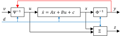
Figure 1: Exactly linearizable model

The HW model refers to the model in which (10) is restricted to the output-independent $u(t)=\Psi^{-1}(v(t),d(t))$. This simple extension allows the model to learn a wider range of dynamical systems than the S–HW model. Further, the S–HW model always has a unique equilibrium corresponding to each input, whereas the EL model can represent systems with multiple equilibria. This difference greatly improves the accuracy of the model but requires more careful treatment during control design.

We attempt to construct EL models introduced in Definition 1 from an input–output data sequence. Recall that functions $\Phi(\cdot,d)$ and $\Psi(\cdot,y,d)$ must be bijective mappings. We parameterize each mapping using a bijective neural network (BNN) (Baird et al., 2005) and a diagonal-BNN, respectively. A BNN represents bijective mapping as the $N$-layered neural network $\Phi(y,d)=\varphi^{(N)}\circ\varphi^{(N-1)}\circ\cdots\circ\varphi^{(1)}(y,d)$, where $\varphi^{(i)}(\cdot,d)(i=1,\ldots,N)$ are parametrized bijective mappings. For example, $\varphi^{(i)}(y,d)=\sinh^{-1}(c^{(i)}(d)+\sinh(W^{(i)}(d)y+b^{i}(d)))$, where $W^{(i)}(d)$ and $b^{(i)}(d),c^{(i)}(d)$ represents matrix-valued and vector-valued functions to be learned. If $W^{(i)}(d)$ is diagonal for all $d\in\mathbb{R}^{l}$ and $i=1,\cdots,N$, the input–output relationship of the BNN becomes element-wise, which we call the diagonal-BNN. Moreover, the function $\Xi(\cdot,\cdot,d)$ must be convex, and we adopt a partially input convex neural network (PICNN) (Amos et al., 2017) for parametrization. The structure of the PICNN is rather complex, and therefore, it is omitted in this paper for simplicity. This model includes many disturbance-dependent parameters such as $A,B,c,W^{(i)},b^{(i)},c^{(i)}(i=1,\cdots,N)$. All these can be arbitrary functions; however, in this study, a standard three-layer fully connected neural network is used to represent each element.

A summary of the superior properties of the EL model is presented below. First, the dynamical system can be considered linear because of the dynamic feedback. Second, the reference for $y$ can be replaced with that for $x$ because of the bijectivity of $\Phi$. Third, the admissible set of $u$ corresponding to the input constraint (1) is convex for any $x$ owing to the element-wise bijectivity of $\Psi$. Finally, the admissible set of $x,u$ corresponding to the output constraint (2) is convex because of the convexity of $\Xi$.

The learning process of the EL model is as follows: The EL model structure is similar to that of the S–HW model (Moriyasu et al., 2022), except that output $y$ is fed back into (10), to use the same procedure for learning the model. The outputs predicted by the model are expressed with a hat to distinguish it from real data. From (10)–(13), we obtain

$$\dot{\hat{y}} ={\left(\frac{\partial\Phi}{\partial y}\right)}^{-1}{\left(A(d)\Phi(y,d)+B(d)\Psi^{-1}(v,y,d)+c(d)-\frac{\partial\Phi}{\partial d}\dot{d}\right)},$$ (14)

$$\hat{z} =\Xi(\Phi(y,d),\Psi^{-1}(v,y,d),d).$$ (15)

A key point is that the bijectivity of the BNN enables these evaluations without using internal signals $x,u$. The data required to evaluate these are those of $v,y,d,\dot{d}$. The prediction error can be evaluated as $e:=[(\dot{\hat{y}}-\dot{y})^{\mathrm{T}},(\hat{z}-z)^{\mathrm{T}}]^{\mathrm{T}}$ using the answer data of $\dot{y},z$. Thus, model learning is reduced to an error minimization problem

$$\mathop{\mathrm{minimize}}\limits_{\theta}\frac{1}{N_{s}}\sum_{i=1}^{N_{s}}e_{i}^{\mathrm{T}}Q_{e}e_{i},$$ (16)

where $N_{s}$, $e_{i}$, $Q_{e}$, and $\theta$ represent the number of sampled data points, prediction error for the $i$ th data point, positive definite matrix, and model parameter vector, respectively.

3 Control Design

In this section, we describe a control method that satisfies constraints (1) and (2) and tracks the output $y$ to the reference value $y_{\mathrm{d}}$. This constrained reference-tracking control can be designed as a convex MPC using the S–HW model; however, the introduction of the output feedback in (10) does not ensure the convexity of the input admissible set in the finite-horizon optimal control problem. In this paper, we propose an alternative design method for an EL model that avoids this problem and attributes the control law to convex optimization instead.

3.1 Tracking Control

From the bijectivity of $\Phi$ and $\Psi$ in Definition 1, the tracking control problem for $y$ (using input $v$) can be reduced to a linear control problem for $x$ (using input $u$) for which the optimal design methods are well developed. For the simplicity of discussion, disturbance $d$ is assumed to be constant in the transformed linear dynamics in (10)–(12), such that

$$\dot{x} =A(\bar{d})x+B(\bar{d})u+c(\bar{d}),$$

$$x =\Phi(y,\bar{d}),\ u=\Psi^{-1}(v,y,\bar{d}).$$

Suppose that $y_{\mathrm{d}}$ is realizable as a steady state with $d=\bar{d}$; then, there exists $u_{\mathrm{d}}$ such that

$$A(\bar{d})x_{\mathrm{d}}+B(\bar{d})u_{\mathrm{d}}+c(\bar{d})=0,\ x_{\mathrm{d}}:=\Phi(y_{\mathrm{d}},\bar{d}).$$ (17)

We consider the control input $u(t)$ for the linear part that minimizes the cost function

$$J:=\int_{0}^{\infty}\tilde{x}^{\mathrm{T}}Q\tilde{x}+\tilde{u}^{\mathrm{T}}R\tilde{u}\ \mathrm{d}t$$ (18)

where $\tilde{x}:=x-x_{\mathrm{d}},\ \tilde{u}:=u-u_{\mathrm{d}}$. The optimal $u$ is given by a linear quadratic regulator

$$u=u_{\mathrm{d}}-K\tilde{x},\ K\coloneqq R^{-1}B^{\mathrm{T}}P$$ (19)

where $P$ represents a unique positive definite solution for the matrix Riccati equation

$$PA+A^{\mathrm{T}}P-PBR^{-1}B^{\mathrm{T}}P+Q=0.$$ (20)

The control input $v(t)$ is obtained by performing an inverse transformation of (10) for the control input $u(t)$ in (19).

The overall flow of the calculation of the control input $v(t)$ is shown in Fig. 3. The controller calculates the control input $v(t)$ from the output signal $y(t)$ obtained from the system to be controlled and the desired target value $y_{\mathrm{d}}$. In the controller, the output signal $y(t)$ is converted into the state variable $x(t)$ through the bijective map $\Phi$, and the internal input signal $u(t)$, which is linearly related to $x(t)$, is obtained using the linear control method (19). In addition, the control input $v(t)$ is obtained by mapping the internal input signal $u(t)$ using the bijective map $\Psi$.

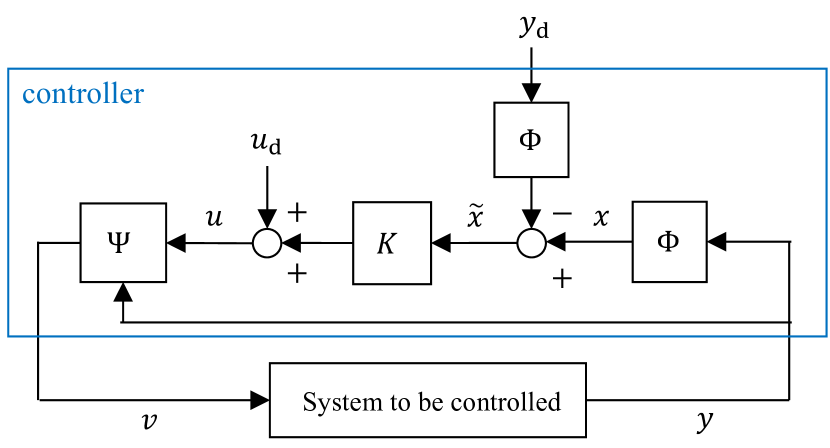
Figure 2: Controller implementation

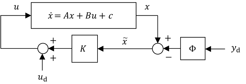
Figure 3: Controller design

Fig. 3 shows the resulting closed-loop system comprising Figs. 1 and 3, which perform feedback control on the linear dynamics $\dot{x}=Ax+Bu+c$. The structure is only a linear system in which the bijective maps $\Psi^{-1}$ and $\Phi^{-1}$ on both sides disappear. Figs. 3 and 3 omit the disturbance $\bar{d}$. The nonlinear optimal control theory can be employed for a more advanced control law than the linear feedback described here; see Appendix 2.

3.2 Constraint-Aware Control

Thus far, constraints (1) and (2) have not been considered. We introduce the control barrier function as one of the methods to satisfy these constraints.

Let us consider an input-affine nonlinear system

$$\dot{x} =f(x)+g(x)u,$$ (21)

$$z^{\prime} =h(x)$$ (22)

with $x\in X(\subset\mathbb{R}^{n}),u\in U(\subset\mathbb{R}^{m}),z^{\prime}\in\mathbb{R},h:X\rightarrow\mathbb{R}$. Note that (21) corresponds to (9) when applied to our EL models, and $U$ corresponds to the input constraint (1).

A continuous and differentiable function $h:X\rightarrow\mathbb{R}$ is called a control barrier function (CBF) if a class $\mathcal{K}_{\infty}$ function is $\alpha:\mathbb{R}_{\geq 0}\rightarrow\mathbb{R}_{\geq 0}$ such that $\sup_{u\in U}\left\{\mathcal{L}_{f}h(x)+\mathcal{L}_{g}h(x)u\right\}\leq\alpha(-h(x))$ for any $x\in X$, where $\mathcal{L}_{f}h(x):=\frac{\partial h}{\partial x}f(x)$. We can verify that if $x(0)\in\{x\in X:h(x)\leq 0\}=:\mathcal{C}$ and $u(t)$ is chosen such as $\mathcal{L}_{f}h(x)+\mathcal{L}_{g}h(x)u\leq\alpha(-h(x))$ for any $t$, then $x(t)$ does not exit $\mathcal{C}$. To employ this property for the required constraint satisfaction, we can use the solution $u^{*}$ for the quadratic optimization

$$\begin{cases}u^{\ast}=&\mathop{\mathrm{arg~{}min}}\limits_{u\in U}\|u-k(x)\|^{2}\\ \mathrm{s.t.}&\mathcal{L}_{f}h(x)+\mathcal{L}_{g}h(x)u\leq\alpha(-h(x))\end{cases}$$ (23)

as a control input, where $k(x)$ is a desirable control law, such as LQR (19). Thus, the output constraint $z^{\prime}=h(x)\leq 0$ is satisfied. In the above description, the constrained output $z^{\prime}$ is assumed to be scalar for simplicity; however, it can be easily extended to a vector by replicating the function $h$.

We consider setting $h(x,u)=\Xi(x,u)-\bar{z}=:h_{z}(x,u)$ to handle output constraint (2). However, the aforementioned framework is not directly applicable to this function because of the input dependency of $\Xi$, and the above discussion is only valid if $h$ depends only on $x$. To circumvent this issue, we restrict input signals to continuously differentiable ones, such as

$$\dot{u}=\lambda,$$ (24)

which is not restrictive for practical applications. The augmented system can then be written as

$$\frac{\mathrm{d}}{\mathrm{d}t}\begin{pmatrix}x\\ u\\ \end{pmatrix} =\begin{pmatrix}f(x)+g(x)u\\ \lambda\\ \end{pmatrix},$$ (25)

$$z^{\prime} =h(x,u).$$ (26)

Considering an augmented vector $[x^{\mathrm{T}},u^{\mathrm{T}}]^{\mathrm{T}}$ as a state and $\lambda$ as a new input, this system falls into the standard CBF framework because the input dependence of $h$ can be eliminated. The CBF obtained by this augmentation is called the integral CBF (I-CBF) (Ames et al., 2021). From a different perspective, the adoption of I-CBF allows the model to have an input dependence on the function $\Xi$. This motivated us to solve this problem

$$\begin{cases}\lambda^{\ast}=&\mathop{\mathrm{arg~{}min}}\limits_{\lambda}\frac{\mathrm{d}}{\mathrm{d}t}\|u-k(x)\|^{2}+a\|\lambda\|^{2}\\ \mathrm{s.t.}&\frac{\partial h}{\partial x}(f(x)+g(x)u)+\frac{\partial h}{\partial u}\lambda\leq\alpha(-h(x,u))\end{cases}$$ (27)

with a positive constant $a$. The first term aims at the quick convergence of $u$ to $k(x)$, and the second term is added to regularize the derivative of the input $u$. Although the input constraint $u\in U$ originally considered in (23) disappears in the above problem, it can be treated using this I-CBF approach. We can combine the vector function

$$h_{v}(x,u):=\begin{bmatrix}u-\Psi^{-1}(\bar{v},\Phi^{-1}(x))\\ \Psi^{-1}(\underline{v},\Phi^{-1}(x))-u\end{bmatrix}$$ (28)

to $h(x,u)$ for handling the input constraint (1). In summary, this approach can handle the constraints (1) and (2) by setting $h(x,u)=[h_{z}(x,u)^{\mathrm{T}},h_{v}(x,u)^{\mathrm{T}}]^{\mathrm{T}}$.

The function to be minimized in (27) is quadratic with respect to $\lambda$, and it is given by

$$F(\lambda) :=\frac{\mathrm{d}}{\mathrm{d}t}\|u-k(x)\|^{2}+a\|\lambda\|^{2}$$ (29)

$$=a\|\lambda\|^{2}+2(u-k(x))^{\mathrm{T}}\lambda-2(u-k(x))^{\mathrm{T}}\frac{\partial k(x)}{\partial x}(f(x)+g(x)u).$$

In addition, any constraint expressed in the form $h(x,u)\leq 0$ is reduced to the affine constraint for $\lambda$ in the I-CBF approach. Thus, the above optimization problem is QP and can be solved quickly using many ready-made solvers. Further, the EL model allows functions $h(x,u)$ corresponding to (1) and (2) to be convex to $u$ for any fixed $x$. This guarantees that $x,u$ at the equilibrium point of this system is the solution to the problem $\mathop{\mathrm{minimize}}\limits_{u}\|u-k(x)\|^{2}\ \mathrm{s.t.}\ h(x,u)\leq 0$ (See Appendix 3).

4 Experimental Evaluation

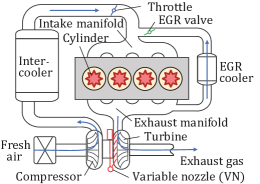
Figure 4: Engine air path and combustion system

The modeling accuracy of the proposed model and the control results are presented using an engine air path and combustion system, as shown in Fig. 4. The system included an internal combustion controller. The physical quantities of each variable are as follows: The output $y:=\left[y_{1},y_{2},y_{3}\right]$ is the net torque $\left[\mathrm{Nm}\right]$, the NOx concentration $\left[\log_{10}(\mathrm{ppm})\right]$, and the generated soot quantity $\left[\mathrm{filtered\ smoke\ number}\right]$. The constraint outputs $z:=\left[z_{1},z_{2}\right]$ are the combustion noise $\left[\mathrm{dB}\right]$ and maximum cylinder pressure $\left[\mathrm{MPa}\right]$, respectively. The inputs $v:=\left[v_{1},v_{2},v_{3}\right]$ are the variable nozzle (VN) closing degree $\left[\mathrm{\%}\right]$, throttle closing degree $\left[\mathrm{\%}\right]$, and exhaust gas recirculation (EGR) valve opening degree $\left[\mathrm{\%}\right]$. The disturbances $d:=\left[d_{1},d_{2}\right]$ are the engine speed $\left[\mathrm{rpm}\right]$ and fuel injection rate $\left[\mathrm{mm^{3}}\right]$, respectively.

The learning results are compared with those of the S–HW model (Moriyasu et al., 2022), EL model A (constraint output $z$ is independent of the internal input $u$), and EL model B (constraint output $z$ depends on the internal input $u$). The response results $\left\{y,z\right\}$ of each model to the input data $\left\{v,d\right\}$ are shown in Fig. 7, and the comparison of the decision coefficients $R^{2}$ is listed in Table 7. Fig. 7 shows that the response of the EL model (A, B) is qualitatively better fitted to real data than that of the S–HW model. Table 7 shows that there is a large difference in the coefficient of determination of the output $y$ between the S–HW and EL models (A, B). The results confirm that the modeling accuracy can be improved by adding the dependency of the internal input $u$ on the constraint output $z$.

We also present the control results for the EL model (B). In this study, we performed optimal control using the methods described in 3.1 and 3.2. That is, we solve QP (27) to calculate the control input online, where $k(x)$ represents LQR (19). The sampling time is $0.001\,\mathrm{sec}$ and the input and output constraints represented by (1) and (2) are $0\leq v_{i}\leq 100\,(i=1,\ldots,3)$ and $z_{1}\leq 80,z_{2}\leq 6.5$. In addition, the class $\mathcal{K}_{\infty}$ functions $\alpha_{i},\alpha_{j}\,(i=1,\ldots 3,j=1,2)$ in (27) are quadratic. The numerical results are shown in Figs. 7 and 7. In these figures, each result and color scheme are shown below.

• Reference $y_{\mathrm{d}}$ for the output $y$ (black solid),

• Bounds for the input $v$ and output $z$ (black dashed),

• Result of unconstrained control by LQR (19) (blue),

• Result of constrained control by QP (27) (green).

Therefore, QP realized the tracking control of output $y$ to the reference $y_{\mathrm{d}}$ while satisfying constraints (1) and (2). For input $v$, the control law based on (19) (blue line) fails to satisfy the constraint (1) (black dashed line), whereas the control law based on QP (green line) is within the constraints. For output $y$, the results of the QP deviate slightly from the reference $y_{\mathrm{d}}$ because there is no input $v$ such that $u=\Psi^{-1}(v,y_{\mathrm{d}},\bar{d})$ satisfies constraints (1) and (2). In other words, from (17), it is possible to obtain $x_{\mathrm{d}}$ and $u_{\mathrm{d}}$ corresponding to $y_{\mathrm{d}}$; however, the $v,z$ obtained by $\Psi$ in (10) and $\Xi$ in (13) do not satisfy the constraints (1), (2). Fig. 7 suggests that our proposed method automatically find a suitable steady input $v$ that achieves good tracking performance for the target $y_{\mathrm{d}}$ while satisfying constraints (1) and (2), which is the purpose of this study.

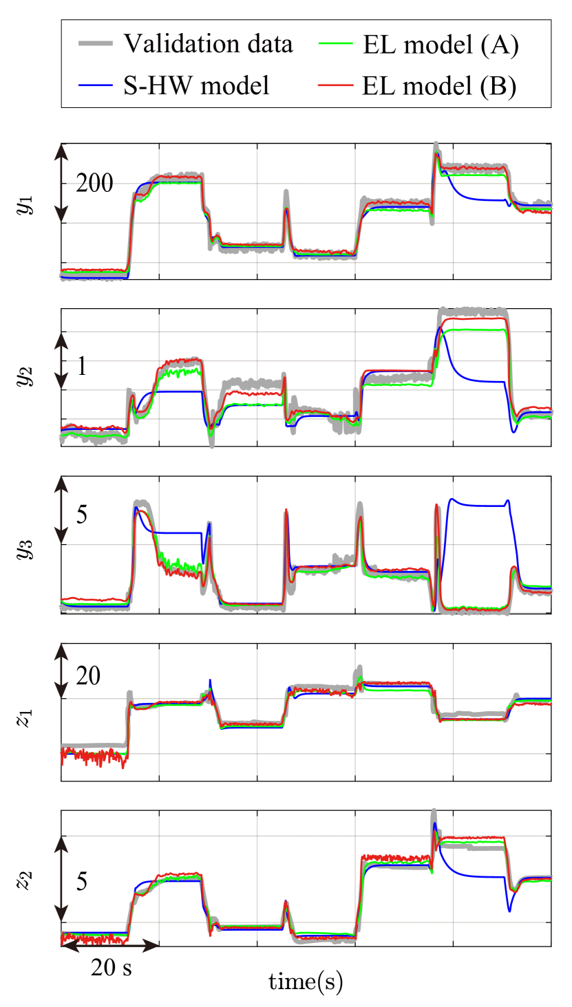
Figure 5: Results of model prediction

Table 1: Coefficient of determination $R^{2}$

	S–HW	EL(A)	EL(B)
$y_{1}$	0.968	0.974	0.976
$y_{2}$	0.841	0.905	0.948
$y_{3}$	0.802	0.960	0.956
$z_{1}$	0.883	0.890	0.925
$z_{2}$	0.947	0.966	0.970
Average	0.888	0.939	0.955

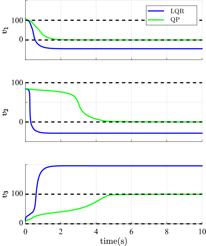
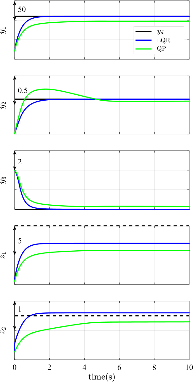
Figure 6: Control result of input $v$

Figure 7: Control result of output $y,z$

5 Conclusion

We extended the S–HW model proposed by Moriyasu et al. (2022) in terms of modeling and control design by proposing the output feedback for the input transformation $\Psi$ in modeling and by introducing an integral control barrier function (Ames et al., 2021) in the control. The experimental validation confirmed the improvement in modeling accuracy, which led to better control. However, the model structure proposed in this study did not cover the full range of linearizable classes. Our future work will cover a wider range of representational capabilities within the class and extensions to a wider class of dynamical systems that encompass the exactly linearizable class.

Appendix 1. Exactly Linearizable Condition (Su, 1982)

In this section, we provide the necessary and sufficient conditions for exact linearizability introduced in Section 2.2. The system of interest is represented by

$$\frac{dy}{dt}=\overline{f}(y)+\overline{g}(y)v.$$ (30)

However, we consider a single-input system ($v\in\mathbb{R}$) for simplicity. Exact linearization implies that we can transform (30) into the following linear system by applying a coordinate transformation (4) and feedback (5)

$$\frac{dx}{dt}=\begin{pmatrix}0&1&0&\cdots&0\\ 0&0&1&\cdots&0\\ \vdots&\vdots&&\ddots&0\\ 0&0&0&\cdots&1\\ 0&0&0&\cdots&0\end{pmatrix}x+\begin{pmatrix}0\\ 0\\ \vdots\\ 0\\ 1\end{pmatrix}u.$$ (31)

In addition, we define two notations.

Definition 2.

From (30), for functions $\overline{f},\overline{g}$, we define the operator $\mathbf{ad}_{\overline{f}}\overline{g}$ as We also refer to $\left[\overline{f},\overline{g}\right]$ as the lie brackets.

$$\mathbf{ad}_{\overline{f}}\overline{g} :=\left[\overline{f},\overline{g}\right],$$ (32)

$$\left[\overline{f},\overline{g}\right] :=\frac{\partial\overline{g}}{\partial y}\overline{f}(y)-\frac{\partial\overline{f}}{\partial y}\overline{g}(y).$$ (33)

Subsequently, the operator (32) acts as

$$\mathbf{ad}^{k+1}_{\overline{f}}\overline{g} =\left[\overline{f},\mathbf{ad}^{k}_{\overline{f}}\overline{g}\right],$$ (34)

$$\mathbf{ad}^{0}_{\overline{f}}\overline{g} =\overline{g}(y),$$ (35)

$$\mathcal{L}_{\mathbf{ad}_{\overline{f}}\overline{g}}\phi(y) =\mathcal{L}_{\overline{f}}\mathcal{L}_{\overline{g}}\phi(y)-\mathcal{L}_{\overline{g}}\mathcal{L}_{\overline{f}}\phi(y),$$ (36)

where $\phi(y)$ denotes the arbitrary function $y$.

The necessary and sufficient conditions for exact linearizability can be expressed as follows:

Theorem 3.

A necessary and sufficient condition for the existence of coordinate transformation (4) and feedback (5) that transform the equation of state (30) into a linear system (31) is the simultaneous satisfaction of the following two conditions:

1. $\left\{\mathbf{ad}^{0}_{\overline{f}}\overline{g},\mathbf{ad}^{1}_{\overline{f}}\overline{g},\cdots,\mathbf{ad}^{n-1}_{\overline{f}}\overline{g}\right\}(y)$ is linearly independent for any $y$.
   

2. $\left\{\mathbf{ad}^{0}_{\overline{f}}\overline{g},\mathbf{ad}^{1}_{\overline{f}}\overline{g},\cdots,\mathbf{ad}^{n-2}_{\overline{f}}\overline{g}\right\}(y)$ is involutive.

In this theorem, 1 is a condition for system controllability, and 2 provides the necessary and sufficient conditions for the unique existence of the coordinate transformation (4) and feedback (5) when 1 is satisfied by the Frobenius’ theorem (Su, 1982).

Appendix 2. Nonlinear Optimal Control for Exactly Linearizable Input-Affine Dynamics

We proposed a control design method that fully utilizes simple linear optimal control theory. In this section, we show how to utilize nonlinear optimal control theory based on the modeling framework in the present study, assuming that the system to be controlled is an input-affine nonlinear system.

Let us consider the following input-affine nonlinear system, as in (4) and (5). We can construct $\Psi_{1},\ \Psi_{2},\ A,\ B,\ c$ as

$$v(t) =\Psi_{1}(y(t))+\Psi_{2}(y(t))u(t),$$ (37)

$$\dot{x}(t) =Ax(t)+Bu(t)+c,$$ (38)

$$y(t) =\Phi^{-1}(x(t)),$$ (39)

using the data for $\{v,y,\dot{y}\}$, where $\Phi$ is bijective and $\Psi_{2}(y)$ is nonsingular for any $y$. Without the loss of generality, we assume $\Phi(0)=0$ and $c=0$. The obtained dynamics are input affines in the form of (3). Next, we define the control Lyapunov function (CLF), which is essential for explaining the Sontag-type stabilizing control law.

Definition 4 (Ames et al. (2019)).

A positive definite function $V:Y\rightarrow\mathbb{R}$ is called a CLF if there exists a class $\mathcal{K}$ function $\gamma$ such that

$$\inf_{v\in D}\left\{\mathcal{L}_{\bar{f}}V(y)+\mathcal{L}_{\bar{g}}V(y)v\right\}<-\gamma(V(y)).$$ (40)

For our model, we explicitly provide the CLF

$${V}(y)=\Phi(y)^{\mathrm{T}}P\Phi(y)$$ (41)

with the solution $P$ to (20). Once a CLF is found, we utilize several tools from the nonlinear control theory.

Theorem 5 (Sontag (1998)).

Let a positive definite function $V:Y\rightarrow\mathbb{R}$ be a CLF for system (3); then, the following Sontag-type control law $u=\alpha_{d}(y)$ asymptotically stabilizes the origin of the system (3).

$$u =\alpha_{d}(y)$$ (42)

$$\alpha_{d}(y) :=\begin{cases}-\frac{1}{r_{d}(y)}(\mathcal{L}_{g}V)^{\mathrm{T}},\ \ &(\mathcal{L}_{g}V\neq 0)\\ 0,&(\mathcal{L}_{g}V=0)\end{cases}$$ (43)

where the bounded function $r_{d}(y)>0$ is given by

$$r_{d}(y):=\frac{\mathcal{L}_{g}V(\mathcal{L}_{g}V)^{\mathrm{T}}}{\mathcal{L}_{f}V+\sqrt{\mathcal{L}_{f}V^{2}+(\mathcal{L}_{g}V(\mathcal{L}_{g}V)^{\mathrm{T}})^{2}}}.$$ (44)

This control law not only stabilizes, but also satisfies the inverse optimality for nonlinear dynamics (Khalil, 2002). This property makes the control law robust, as in the phase margin of the linear control theory. For a more extended framework, please refer to differential flatness (Fliess et al., 1995).

Appendix 3. Equilibrium Condition of Proposed Control System

The system proposed in Section 3.2 can be summarized as

$$\frac{\mathrm{d}}{\mathrm{d}t}\begin{pmatrix}x\\ u\\ \end{pmatrix}=\begin{pmatrix}f(x)+g(x)u\\ \lambda\\ \end{pmatrix},$$ (45)

$$\begin{cases}\lambda^{\ast}=&\mathop{\mathrm{arg~{}min}}\limits_{\lambda}\frac{\mathrm{d}}{\mathrm{d}t}\|u-k(x)\|^{2}+a\|\lambda\|^{2}\\ \mathrm{s.t.}&\frac{\partial h}{\partial x}(f(x)+g(x)u)+\frac{\partial h}{\partial u}\lambda\leq\alpha(-h(x,u))\end{cases},$$ (46)

where $a>0$ and $h(x,u)$ are convex with respect to $u$, for any fixed $x$. The convexity originated from the structure of the EL model. We can prove the optimality of the equilibrium as

Theorem 6.

If an equilibrium point $(x,u)$ exists in the system shown in (45) and (46), then the points satisfy $u=\mathop{\mathrm{arg~{}min}}\limits_{u}\|u-k(x)\|^{2}\ \mathrm{s.t.}\ h(x,u)\leq 0$.

Proof.

As the problem in (46) is strongly convex with $a>0$, the necessary and sufficient condition for first-order optimality can be written as

$$\nabla F(\lambda)+{\left(\nabla G(\lambda)\right)}^{\mathrm{T}}\mu=0,$$ (47)

$$\mu\geq 0,\ G(\lambda)\leq 0,\ \mu\circ G(\lambda)=0,$$ (48)

where $F(\lambda):=\frac{\mathrm{d}}{\mathrm{d}t}\|u-k(x)\|^{2}+a\|\lambda\|^{2},\ G(\lambda):=\frac{\partial h}{\partial x}(f(x)+g(x)u)+\frac{\partial h}{\partial u}\lambda-\alpha(-h(x,u))$, and $\mu$ represents a Lagrange multiplier. Considering the equilibrium condition of (45), i.e., $f(x)+g(x)u=0,\ \lambda=0$, the above optimality condition reduces to

$$2(u-k(x))+{\left(\frac{\partial h}{\partial u}\right)}^{\mathrm{T}}\mu=0,$$ (49)

$$\mu\geq 0,\ h(x,u)\leq 0,\ \mu\circ h(x,u)=0.$$ (50)

$h(x,u)$ is convex to $u$, and therefore, the above condition coincides with the necessary and sufficient condition of the first-order optimality of the optimization problem

$$\mathop{\mathrm{minimize}}\limits_{u}\|u-k(x)\|^{2}\ \mathrm{s.t.}\ h(x,u)\leq 0.$$ (51)

∎

References

- Ames et al. (2019) Aaron D. Ames, Samuel Coogan, Magnus Egerstedt, Gennaro Notomista, Koushil Sreenath, and Paulo Tabuada. Control Barrier Functions: Theory and Applications. 2019 18th European Control Conference (ECC), pages 3420–3431, jun 2019. doi: 10.23919/ECC.2019.8796030.
- Ames et al. (2021) Aaron D. Ames, Gennaro Notomista, Yorai Wardi, and Magnus Egerstedt. Integral control barrier functions for dynamically defined control laws. IEEE Control Systems Letters, 5(3):887–892, 2021. doi: 10.1109/LCSYS.2020.3006764.
- Amos et al. (2017) Brandon Amos, Lei Xu, and J. Zico Kolter. Input convex neural networks. 34th International Conference on Machine Learning, ICML 2017, 1:192–206, 2017.
- Baird et al. (2005) Leemon Baird, David Smalenberger, and Shawn Ingkiriwang. One-step neural network inversion with PDF learning and emulation. In Proceedings. 2005 IEEE International Joint Conference on Neural Networks, 2005., volume 2, pages 966–971. IEEE, 2005. doi: 10.1109/IJCNN.2005.1555983.
- Cervantes et al. (2003) Ania Lussón Cervantes, Osvaldo E. Agamennoni, and José L. Figueroa. A nonlinear model predictive control system based on wiener piecewise linear models. Journal of Process Control, 13(7):655–666, 2003. doi: https://doi.org/10.1016/S0959-1524(02)00121-X.
- Chen et al. (2019) Yize Chen, Yuanyuan Shi, and Baosen Zhang. Optimal control via neural networks: A convex approach. 7th International Conference on Learning Representations, ICLR 2019, pages 1–25, 2019.
- Fliess et al. (1995) Michel Fliess, Jean Levine, Philippe Martin, and Pierre Rouchon. Flatness and defect of non-linear systems: Introductory theory and examples. International Journal of Control, 61(6):1327–1361, 1995. ISSN 13665820. doi: 10.1080/00207179508921959.
- Fruzzetti et al. (1997) Keith P. Fruzzetti, Ahmet N. Palazoğlu, and Karen A. McDonald. Nolinear model predictive control using hammerstein models. Journal of Process Control, 7(1):31–41, 1997. ISSN 0959-1524. doi: https://doi.org/10.1016/S0959-1524(97)80001-B.
- Gros (2019) Sebastien Gros. Implicit non-convex model predictive control. In Handbook of Model Predictive Control, pages 305–333. Springer, 2019.
- Hammerstein (1930) A. Hammerstein. Nichtlineare integralgleichung nebst anwendungen. Acta Mathematica, 54:117–176, 1930.
- Hedjar (2013) Ramdane Hedjar. Adaptive neural network model predictive control. International Journal of Innovative Computing, Information and Control, 9:1245–1257, 01 2013.
- Khalil (2002) Hassan K. Khalil. Nonlinear Systems. Prentice Hall, 3rd ed edition, 2002.
- Kocijan et al. (2004) Juš Kocijan, Roderick Murray-Smith, Carl Edward Rasmussen, and Agathe Girard. Gaussian process model based predictive control. In 2004 American Control Conference, page ThA08.3, 2004.
- Ławryńczuk (2008) Maciej Ławryńczuk. Suboptimal Nonlinear Predictive Control Based on Neural Wiener Models. In Artificial Intelligence: Methodology, Systems, and Applications, pages 410–414. Springer Berlin Heidelberg, Berlin, Heidelberg, 2008. doi: 10.1007/978-3-540-85776-1“˙40.
- Lenz et al. (2015) Ian Lenz, Ross Knepper, and Ashutosh Saxena. DeepMPC: Learning deep latent features for model predictive control. Robotics: Science and Systems, 11, 2015. doi: 10.15607/RSS.2015.XI.012.
- Moriyasu et al. (2019) Ryuta Moriyasu, Sayaka Nojiri, Akio Matsunaga, Toshihiro Nakamura, and Tomohiko Jimbo. Diesel engine air path control based on neural approximation of nonlinear MPC. Control Engineering Practice, 91(April):104114, 2019. doi: 10.1016/j.conengprac.2019.104114.
- Moriyasu et al. (2022) Ryuta Moriyasu, Taro Ikeda, Sho Kawaguchi, and Kenji Kashima. Structured Hammerstein-Wiener Model Learning for Model Predictive Control. IEEE Control Systems Letters, 6:397–402, 2022. ISSN 2475-1456. doi: 10.1109/LCSYS.2021.3077201.
- Nghiem (2019) Truong X. Nghiem. Linearized Gaussian processes for fast data-driven model predictive control. In 2019 American Control Conference, pages 1629–1634, 2019.
- Sontag (1998) Eduardo Sontag. Mathematical Control Theory: Deterministic Finite-Dimensional Systems. 01 1998. doi: 10.1007/978-1-4612-0577-7.
- Su (1982) Renjeng Su. On the linear equivalents of nonlinear systems. Systems & Control Letters, 2(1):48–52, 1982. ISSN 0167-6911. doi: https://doi.org/10.1016/S0167-6911(82)80042-X.
- Wiener (1958) Norbert Wiener. Nonlinear problems in random theory. Wiley, 1958.