Harnessing graph state resources for robust quantum magnetometry under noise

Abstract

Precise measurement of magnetic fields is essential for various applications, such as fundamental physics, space exploration, and biophysics. Although recent progress in quantum engineering has assisted in creating advanced quantum magnetometers, there are still ongoing challenges in improving their efficiency and noise resistance. This study focuses on using symmetric graph state resources for quantum magnetometry to enhance measurement precision by analyzing the estimation theory under Markovian and non-Markovian noise models. The results show a significant improvement in estimating both single and multiple Larmor frequencies. In single Larmor frequency estimation, the quantum Fisher information spans a spectrum from the standard quantum limit to the Heisenberg limit within a periodic range of the Larmor frequency, and in the case of multiple Larmor frequencies, it can exceed the standard quantum limit for both Markovian and non-Markovian noise. This study highlights the potential of graph state-based methods for improving magnetic field measurements under noisy environments.

I Introduction

Quantum sensing utilizes quantum resources like non-classical states, entanglement, and squeezing to improve sensor capabilities beyond classical approaches Degen et al. (2017). Recent advances in quantum resource theory have been made in quantum-enhanced sensing using non-classical states Chalopin et al. (2018); Pezzè et al. (2018); Ho and Kondo (2019), entangled cluster and graph states Friis et al. (2017); Shettell and Markham (2020); Wang and Fang (2020); Le et al. (2023), many-body nonlocality and multiqubit systems Niezgoda and Chwedeńczuk (2021); Chu et al. (2023); Avdic et al. (2023), and squeezed resources Zhang and Duan (2014); Maccone and Riccardi (2020); Gessner et al. (2020); Troullinou et al. (2023). Furthermore, various techniques like machine learning algorithms Cimini et al. (2019); Jung et al. (2021); Costa et al. (2021); Cimini et al. (2023); Rinaldi et al. (2023), quantum error correction methods Kessler et al. (2014); Shettell et al. (2021); Yamamoto et al. (2022); Rojkov et al. (2022), network sensing Proctor et al. (2018); Rahim et al. (2023), and hybrid algorithms Koczor et al. (2020); Yang et al. (2021); Kaubruegger et al. (2021); Meyer et al. (2021); Marciniak et al. (2022); Le et al. (2023); Kaubruegger et al. (2023), are being explored for enhancing noise resilience and extracting insights from quantum sensing.

In quantum magnetometry, the precise measurement of magnetic fields is crucial in various subjects like fundamental physics research, space exploration, material science, geophysics, and medical biophysics. Recent advances in quantum engineering have led to the development of various quantum magnetometers, such as superconducting quantum interference device (SQUID) Portolés et al. (2022), diamond-based magnetometer Gulka et al. (2021); Carmiggelt et al. (2023), single-spin quantum magnetometer Huxter et al. (2022), submicron-scale NMR spectroscopy Sahin et al. (2022), cold atom magnetometer Garrido Alzar (2019), and 2D hexagonal boron nitride magnetic sensor Kumar et al. (2022). These innovations find applications in highly sensitive and broadband magnetic field measurements Gulka et al. (2021); Carmiggelt et al. (2023), scanning gradiometry Huxter et al. (2022), low magnetic fields Sahin et al. (2022), navigation Garrido Alzar (2019), and magnetic field imaging Kumar et al. (2022).

Improving the sensitivity of magnetometers is essential for different applications. However, the present methods are insufficient due to high quantum resource efficiency and noise resilience demands. Therefore, there is an urgent requirement for a novel resource that can enable the full potential of quantum magnetometry while being practical for experimental implementation.

Among various candidates, graph states have emerged as a promising avenue in the quest for quantum-enhanced magnetometry. Graph states are particular types of entangled states that can be represented by a graph, where the vertices represent qubits, and the edges represent entangling gates between the qubits Hein et al. (2006, 2004). Due to their multipartite entanglement, they have demonstrated great potential in quantum computation Bell et al. (2014a); Schlingemann and Werner (2001), communication Bell et al. (2014a, b), and metrology Shettell and Markham (2020); Wang and Fang (2020); Le et al. (2023). Within the context of quantum magnetometry, harnessing the capabilities of graph states introduces a novel dimension to the quest for precision and robustness in the presence of noise.

This work explores symmetric graph state resources for robust quantum magnetometry under Markovian and non-Markovian noise. Our approach begins by modeling an ensemble of $N$ spin-1/2 particles as a sensor probe for measuring Larmor frequencies of an external magnetic field. Initially, the probe state is set up in a star-graph configuration, where one vertex (spin particle) is connected to the remaining $N-1$ vertices through CZ gates. We study the influence of noise in the model by analyzing the measurement precision from the perspective of estimation theory and quantum Fisher information.

For uncorrelated probes, the variance of estimating a single phase $\phi$ follows $\Delta^{2}\phi=\mathcal{O}(N^{-1})$, commonly referred to as the standard quantum limit (SQL), whereas for entangled probes, it is possible to reach the Heisenberg limit (HL), where $\Delta^{2}\phi=\mathcal{O}(N^{-2})$ Pezzé and Smerzi (2009); Giovannetti et al. (2004, 2006). However, under Markovian noise, entangled sensors cannot surpass the SQL Huelga et al. (1997); Smirne et al. (2016). In the presence of non-Markovian noise, the variance can reach $\Delta^{2}\phi=\mathcal{O}(N^{-1.5})$ Matsuzaki et al. (2011); Chin et al. (2012); Tanaka et al. (2015), and similar results have been observed in the context of multiphase sensing Ho et al. (2020); Le et al. (2023).

In our investigation for single Larmor frequency estimation, we observe a transition from SQL to HL behavior for a periodic range of the Larmor frequency. For multiple Larmor frequencies, we find that the variance $\Delta^{2}\bm{\phi}$ can beat the SQL for both Markovian and non-Markovian noise sources. This marks the initial instance where we observe surpassing the SQL under Markovian noise. Our analysis of quantum magnetometry in these noise factors sheds light on the resilience and potential of graph state-based approaches for conducting highly precise magnetic field measurements in challenging and real-world conditions.

II Results

II.1 Measurement model and its initialization

Let us consider the measurement of an external magnetic field by employing a spin-1/2 system comprising $N$ particles as the probing mechanism. Each particle interacts with the field and provide information about the field strengths. The coupling Hamiltonian is given by Tekely (2002)

$$\mathcal{H}=-\sum_{k=1}^{N}\Big{(}\bm{\mu}^{(k)}\cdot\bm{B}\Big{)},$$ (1)

where $\bm{\mu}^{(k)}=\frac{1}{2}\gamma_{e}\bm{\sigma}^{(k)}$ represents the magnetic moment of the $k^{\rm th}$ spin. $\gamma_{e}$ denotes the gyromagnetic ratio, and $\bm{\sigma}^{(k)}=\big{(}\sigma_{x}^{(k)},\sigma_{y}^{(k)},\sigma_{z}^{(k)}\big{)}$ refers to the Pauli matrices. Here, $\bm{B}=(B_{x},B_{y},B_{z})$ signifies the external magnetic field. We define $\phi_{j}=|\gamma_{e}|B_{j}$ for all $j\in{x,y,z}$ as the Larmor frequency Tekely (2002), and $J_{j}=\frac{1}{2}\sum_{k}\sigma_{j}^{(k)}$ as the angular momentum. With this, the Hamiltonian recasts as

$$\mathcal{H}=\bm{\phi}\cdot\bm{J},$$ (2)

where $\bm{\phi}=(\phi_{x},\phi_{y},\phi_{z})$ represents the set of Larmor frequencies requiring estimation, and $\bm{J}=(J_{x},J_{y},J_{z})$ are three components of the collective angular momentum. Refer to App. A for a detailed model and its quantum circuit.

The probe is initialized as a graph state, which typically consists of a collection of vertices denoted by $V$ and edges represented by $E$ as

$$G(V,E)=\prod_{{i,j}\in E}{\rm CZ}_{ij}|+\rangle^{\otimes V},$$ (3)

where ${\rm CZ}_{ij}$ represents the controlled-Z gate connecting the $i^{\rm th}$ and $j^{\rm th}$ spins, and $|+\rangle$ is an element in the basis of Pauli $\sigma_{x}$. Graph states serve as valuable assets in quantum metrology Shettell and Markham (2020); Le et al. (2023), as demonstrated by their application in achieving Heisenberg scaling, as observed with star configurations where the quantum Fisher information (QFI) gives $(N-1)^{2}+1$, and with local Clifford (LC) operations where the QFI gives $N^{2}$ Shettell and Markham (2020). Hereafter, we examine the impact of graph-state resources on quantum-enhanced magnetometry within a noisy environment.

II.2 Single phase estimation

We examine the estimation of a single Larmor frequency denoted as $\bm{\phi}=(\phi,0,0)$. The coupling Hamiltonian is $\mathcal{H}=\phi J_{x}$, and the corresponding unitary operator is expressed as

$$\mathcal{U}(\phi)=\exp\big{(}-it\phi J_{x}\big{)}.$$ (4)

The initial probe state is prepared in a graph configuration $\rho_{0}=|G\rangle\langle G|$. After the interaction, it evolves to $\rho(\phi)=\mathcal{U}(\phi)\rho_{0}\mathcal{U}^{\dagger}(\phi)$. During the magnetic field coupling, the probe interacts with its surroundings and decoheres. Our analysis focuses on dephasing noise as a type of decoherence that leads to the evolution of the state

$$\rho({\phi,\gamma})=\Big{[}\prod_{k=1}^{N}e^{\gamma t\mathcal{L}^{(k)}}\Big{]}\rho(\phi),$$ (5)

where $\gamma$ is the dephasing rate. By employing the Kraus operators to account for dephasing noise as $\mathcal{K}_{0}={\rm diag}(1,\sqrt{1-\lambda}),\mathcal{K}_{1}={\rm diag}(0,\sqrt{\lambda})$, we obtain

$$e^{\gamma t\mathcal{L}^{(k)}}\rho(\phi)=\mathcal{K}_{0}^{(k)}\rho(\phi)\big{[}\mathcal{K}_{0}^{(k)}\big{]}^{\dagger}+\mathcal{K}_{1}^{(k)}\rho(\phi)\big{[}\mathcal{K}_{1}^{(k)}\big{]}^{\dagger},$$ (6)

where $\lambda=1-e^{-\gamma t}\in[0,1]$ is the dephasing probability. For other noisy scenarios, please see App. D.

The final state $\rho({\phi,\gamma})$ contains detailed information about the unknown Larmor frequency $\phi$. To evaluate the precision of the estimation, we examine the QFI $Q$. By decomposing $\rho({\phi,\gamma})=\sum_{k}\ell_{k}|\ell_{k}\rangle\langle\ell_{k}|$, the QFI yields PARIS (2009)

$$Q=2\sum_{i,j,\ell_{i}+\ell_{j}\neq 0}\dfrac{\big{|}\langle\ell_{i}|\partial_{\phi}\rho({\phi,\gamma})|\ell_{j}\rangle\big{|}^{2}}{\ell_{i}+\ell_{j}}.$$ (7)

For numerical calculation, let us fix the sensing time $t=1$ in an arbitrary unit. The results are presented in Fig. 1, focusing on the star-graph configuration and using $N=5$ as an illustrative example. In the absence of noise, i.e., $\lambda=0$, the QFI yields $Q=(N-1)^{2}+1$ Shettell and Markham (2020), which does not depend on $\phi$ as shown in the dashed red line. However, in the presence of noise, the QFI depends on both $\lambda$ and $\phi$. As $\lambda$ increases, the QFI gradually decreases, reaching its minimum value at $\lambda=1$. Interestingly, this minimum value remains nonzero for $\phi\neq 0$, which is demonstrated by the solid black curve. Specifically, for $\phi=\pi/2$, the QFI is even by $(N-1)^{2}$ (red circle). See App. B for detailed calculation.

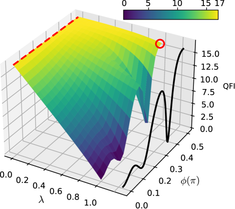
Figure 1: Quantum Fisher information in a single phase estimation. Plot of QFI vs the noise probability $\lambda$ and Larmor frequency $\phi$ for $N=5$ and $t=1$. For $\lambda=0$, the QFI reaches $Q=(N-1)^{2}+1\ \forall\phi$ (dashed red line). Increasing $\lambda$, the QFI gradually reduces and reaches the minimum at $\lambda=1$. Remarkably, this minimum is non-zero for a non-zero $\phi$ as illustrated by the soiled black curve. For $\phi=\pi/2$, it is given by $(N-1)^{2}$ (red circle).

A specific case of star graph is a GHZ state up to a local unitary (LU) transformation Hein et al. (2004); Dür et al. (2003). Let us consider the initial probe state to be a GHZ state

$$|\psi\rangle_{\rm GHZ}=\dfrac{1}{\sqrt{2}}\Big{(}|\nu_{\max}\rangle+|\nu_{\min}\rangle\Big{)},$$ (8)

where $|\nu_{\max}\rangle$ and $|\nu_{\min}\rangle$ are eigenstates of $J_{x}$ corresponding to the maximum and minimum eigenvalues $\nu_{\max}$ and $\nu_{\min}$, respectively. Particularly, this state can be prepared by applying a Hadamard gate to the first spin particle of the star graph state in Eq. (B.1). The QFI gives (see App. B)

$$Q_{\rm GHZ}=N^{2}.$$ (9)

Here, the QFI remains independent of $\phi$. Upon closer examination, it becomes evident that the QFI attains the Heisenberg limit of $N^{2}$ in the absence of noise. In the presence of dephasing noise, the QFI is is invariant, preserving its $N^{2}$ as detailed in App. B. This result is trivial as noise primarily affects the phase or coherence of quantum states along the $z$-axis, while GHZ here points toward the $x$-axis.

Next, we examine the quantum Cramér-Rao bound (QCRB) for various values of $N$. It is the ultimate bound that imposes the precision achievable in the estimation process, i.e, $M\cdot\Delta^{2}\phi\geq\mathsf{C_{F}}\geq\mathsf{C_{Q}}$, where $\Delta^{2}\phi=\langle(\phi-\hat{\phi})^{2}\rangle-\langle(\phi-\hat{\phi})\rangle^{2}$ is the variance of $\phi$, which indicates the difference between the true value $\phi$ and its estimated counterpart $\hat{\phi}$, $M$ is the repeated experiments. Here, $\mathsf{C_{F}}$ and $\mathsf{C_{Q}}$ are classical and quantum Cramér-Rao bound, respectively. The QCRB is determined through the inversion of the QFI as

$$\mathsf{C_{Q}}=Q^{-1},$$ (10)

which can be achieved in the single-phase estimation, such as using a Bayesian estimator or neural network technical (see Rinaldi et al. (2023) and Refs therein).

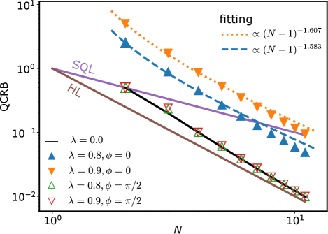
Figure 2: Quantum Cramér-Rao bound in a single phase estimation. The plot of QCRB as a function of the number of spins $N$ for various $\lambda$ and $\phi$. Additionally, SQL and HL are displayed for comparative purposes. The plot is presented with the star-graph configuration.

The numerical results are showcased in Fig. 2. For $\phi=0$, the QCRB can beat the SQL event for large noise. Here we illustrate for $\lambda=0.8$ ($\blacktriangle$) and 0.9 ($\blacktriangledown$), and the fitting curves are proportional to $(N-1)^{-1.583}$ (blue dashed line) and $(N-1)^{-1.607}$ (orange dotted line), respectively. Throughout the paper, we use the fitting function as $f(N)=a(N-1)^{b}\ \forall a,b\in\mathcal{R}$, which is inspired by the exact result when $\lambda=0$. For $\phi=\pi/2$, the analytical findings in Fig. 1 suggest that the QCRB fluctuates between $\frac{1}{(N-1)^{2}+1}$ and $\frac{1}{(N-1)^{2}}$ for $\lambda\in[0,1]$. Comparatively, the cases of $\lambda=0.8$ ($\vartriangle$) and 0.9 ($\triangledown$) align closely with the $\lambda=0$ scenario (the black line), exhibiting a remarkable match. Notably, they attain the Heisenberg scaling. For comparison, we show the standard quantum limit SQL = $N^{-1}$ and the Heisenberg limit HL = $N^{-2}$. This result represents an advanced approach in leveraging graph states for robust sensing in noisy environments, indicating a transition from the SQL to the HL within a periodic range of the Larmor frequency.

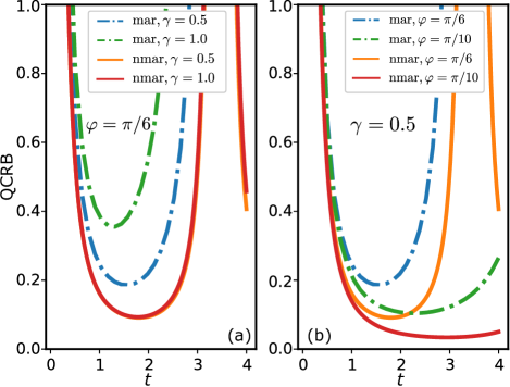
Figure 3: Quantum Cramér-Rao bound in a multiphase estimation. The plot of QCRB as a function of sensing time for Markovian (mar) and non-Markovian (nmar) noises. Here we fixed the Larmor frequencies $\phi_{x}=\phi_{y}=\phi_{z}\equiv\varphi=\pi/6$ in (a) and fixed $\gamma=0.5$ in (b). The QCRB initially decreases, reaches a minimum, and then increases with increasing sensing time.

II.3 Multiple phases estimation

We consider the estimation of Larmor frequencies as $\bm{\phi}=(\phi_{x},\phi_{y},\phi_{z})$ with the coupling Hamiltonian is given in Eq. (2). The unitary evolution yields

$$\mathcal{U}(\bm{\phi})=\exp\big{(}-it\bm{\phi}\cdot\bm{J}\big{)}.$$ (11)

We consider the Ornstein-Uhlenbeck noise model, originating from the stochastic fluctuations of the external magnetic field Uhlenbeck and Ornstein (1930). The noise is characterized by Kraus operators Yu and Eberly (2010)

$$\mathcal{K}_{0}(t)={\rm diag}\big{(}1,\sqrt{1-q(t)}\big{)},\mathcal{K}_{1}(t)={\rm diag}\big{(}0,\sqrt{q(t)}\big{)},$$ (12)

where $q(t)=1-e^{-f(t)}$ and $f(t)=\gamma[t+\tau_{c}(e^{-t/\tau_{c}}-1)]$. Here, $\tau_{c}$ signifies the memory time of the environment. In the limit of Markovian behavior ($\tau_{c}\to 0$), $f(t)=\gamma t$, aligning with the previous dephasing case. In the non-Markovian limit with a large $\tau_{c}$, such as when $t/\tau_{c}\ll 1$, the expression becomes $f(t)=\frac{\gamma t^{2}}{2\tau_{c}}$. The function $q(t)$ is defined as

$$q(t)=\begin{cases}1-\exp(-\gamma t)\;\;\;\;&\textrm{Markovian,}\\ 1-\exp(-\frac{\gamma t^{2}}{2\tau_{c}})\;\;\;&\textrm{non-Markovian.}\end{cases}$$ (13)

For the numerical simulation, $\tau_{c}$ is fixed at $\tau_{c}=20$. Figure 3 illustrates the QCRB concerning Markovian and non-Markovian noises as a function of time $t$. See detailed calculations in App. C. Consistent with findings reported in Ho et al. (2020); Le et al. (2023), a pivotal insight surfaces: an optimal sensing time emerges leads to minimized CRBs across the examined scenarios. For Markovian (mar) noise, the optimal sensing time tends to be shorter, whereas for non-Markovian (nmar) noise, an extended sensing time is favored. Remarkably, the presence of non-Markovian dephasing yields lower metrological bounds compared to the Markovian counterpart.

In Figure 4, we can observe the minimum QCRB for various values of $N$. The results demonstrate that as $N$ increases, non-Markovian noise consistently outperforms the SQL across all levels of noise (represented by open triangles). The relationship follows a fitted function that scales as $\propto(N-1)^{-1.071}$. Similarly, in the case of Markovian noise, the bounds tend to surpass the SQL as $N$ grows larger. This is the first instance we observe exceeding the SQL under Markovian noise.

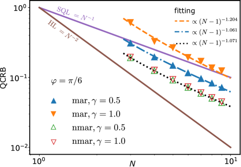
Figure 4: Quantum Cramér-Rao bound in a multiphase estimation. The plot of QCRB vs $N$ at fixed Larmor frequencies $\phi_{x}=\phi_{y}=\phi_{z}\equiv\varphi=\pi/6$ for two cases of Markovian and non-Markovian noise.

III Discussion

We discuss the Bayesian inference in estimating the single Larmor frequency. In this approach, the process begins with defining a likelihood function that expresses the probability of the observed data set $\{D\}$ concerning the parameter of interest $\phi$. In our scenario, the likelihood function is calculated as the product of probabilities while measuring the final state $\rho(\phi,\gamma)$ in Eq. (5) with the computational bases $\{|k\rangle\}$ as

$$P(D|\phi)=\prod_{k=1}^{2^{N}}{\rm Tr}\Big{[}\rho(\phi,\gamma)|k\rangle\langle k|\Big{]}.$$ (14)

The Bayesian theorem is then applied to compute the posterior distribution, which describes the uncertainty associated with the parameter as

$$P(\phi|D)=\dfrac{P(D|\phi)}{\int P(D|\phi)d\phi}.$$ (15)

Finally, the estimated phase is given by

$$\phi_{\rm estimated}=\int\phi P(\phi|D)d\phi.$$ (16)

Practically, sampling techniques such as Markov Chain Monte Carlo (MCMC) or Nested Sampling (NS) are used to generate samples from the posterior distribution Rinaldi et al. (2023). These samples are then used for estimates, typically as the posterior mean or credible intervals. These estimates convey not only the point estimate but also the related uncertainty.

To illustrate, we focus on the case where $\lambda=1$ and proceed to theoretically derive the likelihood function (14) using $\rho_{N}(\phi)$ from Eq.(B.12). The detailed calculation for obtaining the estimated $\phi_{\rm estimated}$ is provided in App. E. We present our findings in Fig. 5. In (a), a comparison is made between the true values and the estimated values. The true values are represented by the blue line when $\phi_{\rm true}=\phi_{\rm estimated}$. The average estimated values are indicated by orange dots with error bars, obtained through the Bayesian inference method from $M=100$ repeated experiments in a quantum circuit. In (b), we plot the squared error $\Delta^{2}\phi$ as a function of $\phi$ and compare it with the inverse QFI extracted from the black curve in Fig. 1 after re-scaling, i.e., $2.5\times\dfrac{1}{MQ}$. It indicates the QCRB relation as $\Delta^{2}\phi\geq\dfrac{1}{MQ}$.

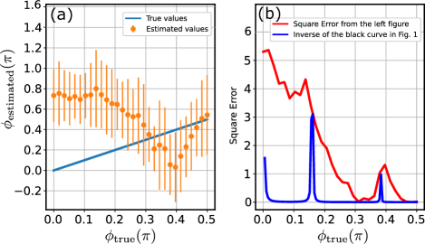
Figure 5: Bayesian inference. (a) A comparison between true and estimated values. The true values are represented by the blue line where $\phi_{\rm true}=\phi_{\rm estimated}$. The estimated values are indicated by orange dots along with error bars, derived from 100 repeated experiments using Bayesian inference. (b) Plot of squared errors as a function of $\phi$ and their comparison with the inverse QFI extracted from the black curve in Fig. 1. These results are presented for $\lambda=1$.

IV Conclusion

Harnessing graph-state resources for robust quantum magnetometry under noise shows promise for overcoming practical measurement challenges. Our demonstrations highlight substantial advancements in accurately measuring both single and multiple Larmor frequencies. These outcomes showcase a spectrum ranging from surpassing the standard quantum limit to achieving Heisenberg scaling, marking significant progress. Further research and development in graph state-based quantum metrology could revolutionize various fields and pave the way for practical quantum technologies despite the noise. We remark that with advancements in experimental generation of arbitrary photonic graph states via atomic Thomas et al. (2022) sources, and quantum-error-correcting code based on graph states Vigliar et al. (2021), this line of research will provide a theoretical basis for quantum-metrological advantages through experiments with graph states.

Appendix A Qubits model

We introduce a measurement model using qubits system. We first rewrite Eq. (11) as

$$\mathcal{U}(\bm{\phi}) =\exp\Big{[}-it(\phi_{x}J_{x}+\phi_{y}J_{y}+\phi_{z}J_{z})\Big{]}$$

$$=\exp\Big{[}-it\sum_{k=1}^{N}\big{(}\frac{\phi_{x}}{2}\sigma_{x}^{(k)}+\frac{\phi_{y}}{2}\sigma_{y}^{(k)}+\frac{\phi_{z}}{2}\sigma_{z}^{(k)}\big{)}\Big{]}$$

$$=\prod_{k=1}^{N}\exp\Big{[}-it(\frac{\phi_{x}}{2}\sigma_{x}^{(k)}+\frac{\phi_{y}}{2}\sigma_{y}^{(k)}+\frac{\phi_{z}}{2}\sigma_{z}^{(k)}\big{)}\Big{]}.$$ (A.1)

We set a single-qubit unitary as

$$\mathcal{U}_{1}(\bm{\phi})=\exp\Big{[}-it(\frac{\phi_{x}}{2}\sigma_{x}+\frac{\phi_{y}}{2}\sigma_{y}+\frac{\phi_{z}}{2}\sigma_{z}\big{)}\Big{]},$$ (A.2)

and apply it to all qubits in a quantum circuit. For a single-phase estimation, it becomes a rotation gate, i.e. $\mathcal{U}_{1}(\bm{\phi})=\exp\big{[}-it\frac{\phi_{x}}{2}\sigma_{x}$].

The quantum circuit is given in Fig. 6. The first block is the graph state generation with start configuration, wherein a Hadamard gate is applied to each qubit initially set in the state $|0\rangle$, transforming them into $|+\rangle$ states. These qubits are connected as a star, with the first qubit at the center and connects to the surrounding qubits through CZ gates. The second block is phase and noise encoding, given by applying $\mathcal{U}_{1}(\bm{\phi})$ and followed by the Kraus operators $\mathcal{K}=(\mathcal{K}_{0},\mathcal{K}_{1})$ apply to all qubits. The final state is used to calculate QFIM and QCRB Ho (2023).

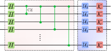
Figure 6: The quantum circuit designed for quantum magnetometry. The first block is a star configuration, applying Hadamard gates to $|0\rangle$ qubits to transform them into $|+\rangle$ states and connecting them as a star, with the first qubit at the center linked to the surrounding qubits via CZ gates. The second block involves phase and noise encoding using $\mathcal{U}_{1}(\bm{\phi})$, followed by Kraus operators $\mathcal{K}=(\mathcal{K}_{0},\mathcal{K}_{1})$ apply to all qubits.

Appendix B Deriving QFI for single parameter estimation

B.1 For star graph state

We first calculate the QFI with the initial star graph state in the case of without noise. We express the QFI in terms of its generator as

$$Q=4\langle\Delta\mathcal{H}^{2}_{\phi}\rangle=4\Big{[}\langle G|\mathcal{H}^{2}_{\phi}|G\rangle-(\langle G|\mathcal{H}_{\phi}|G\rangle)^{2}\Big{]},$$ (B.1)

where $\mathcal{H}_{\phi}=i\mathcal{U}^{\dagger}(\phi)\partial_{\phi}\mathcal{U}(\phi)$. For single-phase estimation, it gives $\mathcal{H}_{\phi}=J_{x}=\frac{1}{2}\sum_{k=1}^{N}\sigma_{x}^{(k)}$.

To calculate Eq. (B.1), we first expand the graph state to a star configuration, with one central qubit (qubit 1) connects to the remaining surrounding $N-1$ qubits:

$$|G\rangle =\prod_{k=2}^{N}{\rm CZ}_{1,k}|+\rangle^{\otimes N}$$

$$=\Big{(}{\rm CZ}_{1,N}{\rm CZ}_{1,N-1}\cdots{\rm CZ}_{1,2}\Big{)}|+\rangle^{\otimes N}$$

$$=\dfrac{1}{\sqrt{2}}\Big{(}|0\rangle|+\rangle^{\otimes(N-1)}+|1\rangle|-\rangle^{\otimes(N-1)}\Big{)}.$$ (B.2)

Next, we compute $\mathcal{H}_{\phi}|G\rangle$:

$$\mathcal{H}_{\phi}|G\rangle =\Big{[}\dfrac{1}{2}\sum_{k=1}^{N}\sigma_{x}^{(k)}\Big{]}|G\rangle$$

$$=\dfrac{1}{2\sqrt{2}}\Big{[}\Big{(}|1\rangle|+\rangle^{\otimes(N-1)}+|0\rangle|-\rangle^{\otimes(N-1)}\Big{)}+$$

$$\hskip 28.45274pt(N-1)\Big{(}|0\rangle|+\rangle^{\otimes(N-1)}-|1\rangle|-\rangle^{\otimes(N-1)}\Big{)}\Big{]}.$$ (B.3)

Using Eq. (B.1), the first term in Eq. (B.1) gives:

$$\langle G|\mathcal{H}^{2}_{\phi}|G\rangle=\langle G|\mathcal{H}_{\phi}\mathcal{H}_{\phi}|G\rangle=\dfrac{1}{4}\Big{(}1+(N-1)^{2}\Big{)}.$$ (B.4)

Using Eqs. (B.1,B.1), the second term in Eq. (B.1) yields

$$\langle G|\mathcal{H}_{\phi}|G\rangle^{2}=0.$$ (B.5)

As a result, the QFI in (B.1) gives

$$Q=1+(N-1)^{2},$$ (B.6)

and the corresponding QCRB is $\mathsf{C_{Q}}=\frac{1}{Q}=\frac{1}{1+(N-1)^{2}}$.

Now, we calculate the QFI under dephasing noise. We first recast the unitary Eq. (4) as

$$\mathcal{U}(\phi) =\Big{[}\exp\big{(}-i\frac{\phi}{2}\sigma_{x}\big{)}\Big{]}^{\otimes N}$$

$$=\Big{[}\cos(\phi^{\prime})I-i\sin(\phi^{\prime})\sigma_{x}\Big{]}^{\otimes N},$$ (B.7)

where we fixed $t=1$ and set $\phi^{\prime}=\phi/2$. The initial graph state $|G\rangle$ evolves to

$$|G(\phi)\rangle =\Big{[}\cos(\phi^{\prime})I-i\sin(\phi^{\prime})\sigma_{x}\Big{]}^{\otimes N}\cdot\dfrac{1}{\sqrt{2}}\Big{(}|0\rangle|+\rangle^{\otimes(N-1)}+|1\rangle|-\rangle^{\otimes(N-1)}\Big{)}$$

$$=\dfrac{1}{\sqrt{2}}\Big{\{}\Big{(}\cos(\phi^{\prime})|0\rangle-i\sin(\phi^{\prime})|1\rangle\Big{)}\otimes e^{-i\phi^{\prime}(N-1)}|+\rangle^{\otimes(N-1)}+$$

$$\hskip 113.81102pt\Big{(}\cos(\phi^{\prime})|1\rangle-i\sin(\phi^{\prime})|0\rangle\Big{)}\otimes e^{i\phi^{\prime}(N-1)}|-\rangle^{\otimes(N-1)}\Big{\}}$$

$$=\dfrac{1}{\sqrt{2}}\Bigg{\{}e^{-i\phi^{\prime}(N-1)}\begin{pmatrix}\cos\phi^{\prime}\\ -i\sin\phi^{\prime}\end{pmatrix}\otimes|+\rangle^{\otimes(N-1)}+e^{i\phi^{\prime}(N-1)}\begin{pmatrix}-i\sin\phi^{\prime}\\ \cos\phi^{\prime}\end{pmatrix}\otimes|-\rangle^{\otimes(N-1)}\Bigg{\}}.$$ (B.8)

The single-qubit dephasing is represented by Kraus operators $\mathcal{K}_{0}={\rm diag}(1,\sqrt{1-\lambda}),\mathcal{K}_{1}={\rm diag}(0,\sqrt{\lambda})$. They act on a qubit $i$ as $\mathcal{K}_{0}^{(i)}=I\otimes\cdots\mathcal{K}_{0}\cdots\otimes I$ and $\mathcal{K}_{1}^{(i)}=I\otimes\cdots\mathcal{K}_{1}\cdots\otimes I$. Under dephasing, the quantum state (6) explicitly gives

$$\rho_{k}(\phi)=\mathcal{K}_{0}^{(k)}\rho_{(k-1)}(\phi)\big{[}\mathcal{K}_{0}^{(k)}\big{]}^{\dagger}+\mathcal{K}_{1}^{(k)}\rho_{(k-1)}(\phi)\big{[}\mathcal{K}_{1}^{(k)}\big{]}^{\dagger},$$ (B.9)

for $k=1,\cdots,N$ with $\rho_{0}(\phi)=|G(\phi)\rangle\langle G(\phi)|$.

To simplify the calculation, we focus on the maximum noise probability, $\lambda=1$. We first calculate

$$\rho_{1}(\phi) =\mathcal{K}_{0}^{(1)}|G(\phi)\rangle\langle G(\phi)|\mathcal{K}_{0}^{(1)}+\mathcal{K}_{1}^{(1)}|G(\phi)\rangle\langle G(\phi)|\mathcal{K}_{1}^{(1)}$$

$$=\dfrac{1}{2}\Bigg{\{}\begin{pmatrix}\cos^{2}\phi^{\prime}&0\\ 0&\sin^{2}\phi^{\prime}\end{pmatrix}\otimes\big{(}|+\rangle\langle+|\big{)}^{\otimes(N-1)}$$

$$+e^{-2i\phi^{\prime}(N-1)}\dfrac{i}{2}\sin(2\phi^{\prime})\sigma_{z}\otimes\big{(}|+\rangle\langle-|\big{)}^{\otimes(N-1)}$$

$$+e^{2i\phi^{\prime}(N-1)}\dfrac{-i}{2}\sin(2\phi^{\prime})\sigma_{z}\otimes\big{(}|-\rangle\langle+|\big{)}^{\otimes(N-1)}$$

$$+\begin{pmatrix}\sin^{2}\phi^{\prime}&0\\ 0&\cos^{2}\phi^{\prime}\end{pmatrix}\otimes\big{(}|-\rangle\langle-|\big{)}^{\otimes(N-1)}\Bigg{\}},$$ (B.10)

Continuously we calculate $\rho_{2}(\phi)$ as:

$$\rho_{2}(\phi) =\mathcal{K}_{0}^{(2)}\rho_{1}(\phi)K_{0}^{(2)}+\mathcal{K}_{1}^{(2)}\rho_{1}(\phi)K_{1}^{(2)}$$

$$=\dfrac{1}{4}\Bigg{\{}\begin{pmatrix}\cos^{2}\phi^{\prime}&0\\ 0&\sin^{2}\phi^{\prime}\end{pmatrix}\otimes I\otimes\big{(}|+\rangle\langle+|\big{)}^{\otimes(N-2)}$$

$$+e^{-2i\phi^{\prime}(N-1)}\dfrac{i}{2}\sin(2\phi^{\prime})\sigma_{z}\otimes\sigma_{z}\otimes\big{(}|+\rangle\langle-|\big{)}^{\otimes(N-2)}$$

$$+e^{2i\phi^{\prime}(N-1)}\dfrac{-i}{2}\sin(2\phi^{\prime})\sigma_{z}\otimes\sigma_{z}\otimes\big{(}|-\rangle\langle+|\big{)}^{\otimes(N-2)}$$

$$+\begin{pmatrix}\sin^{2}\phi^{\prime}&0\\ 0&\cos^{2}\phi^{\prime}\end{pmatrix}\otimes I\otimes\big{(}|-\rangle\langle-|\big{)}^{\otimes(N-2)}\Bigg{\}},$$ (B.11)

and so on. Finally, we get

$$\rho_{N}(\phi)=\dfrac{1}{2^{N}}\Big{(}I^{\otimes N}+\sin(\phi)\sin[(N-1)\phi]\sigma_{z}^{\otimes N}\Big{)}.$$ (B.12)

To calculate the QFI, we use Eq. (7) in the main text with $\rho_{N}({\phi})=\sum_{k}\ell_{k}|\ell_{k}\rangle\langle\ell_{k}|$, and get

$$Q=2\sum_{i,j,\ell_{i}+\ell_{j}\neq 0}\dfrac{\big{|}\langle\ell_{i}|\partial_{\phi}\rho_{N}(\phi)|\ell_{j}\rangle\big{|}^{2}}{\ell_{i}+\ell_{j}}=(N-1)^{2},$$ (B.13)

where we first calculated $\partial_{\phi}\rho_{N}(\phi)$ from Eq. (B.12), and then used $\phi=\pi/2$.

B.2 For GHZ state

We consider the case where the initial probe state is a GHZ state. For the generator $\mathcal{H}_{\phi}=J_{x}=\frac{1}{2}\sum_{k=1}^{N}\sigma_{x}^{(k)}$, the defined GHZ state in Eq. (8) explicitly gives:

$$|\psi_{\rm GHZ}\rangle=\dfrac{1}{\sqrt{2}}\Big{(}|+\rangle^{\otimes N}+|-\rangle^{\otimes N}\Big{)},$$ (B.14)

where $|\pm\rangle^{\otimes N}$ are eigenstates of $\mathcal{H}_{\phi}$ corresponds to the maximum and minimum eigenvalues. This state can be prepared from a star-graph state by adding a Hadamard gate into the first qubits of Eq. (B.1).

We first compute two terms $\mathcal{H}_{\phi}|\psi_{\rm GHZ}\rangle$ and $\mathcal{H}^{2}_{\phi}|\psi_{\rm GHZ}\rangle$, where

$$\mathcal{H}_{\phi}|\psi_{\rm GHZ}\rangle =\Big{[}\dfrac{1}{2}\sum_{k=1}^{N}\sigma_{x}^{(k)}\Big{]}\frac{1}{\sqrt{2}}\Big{(}|+\rangle^{\otimes N}+|-\rangle^{\otimes N}\Big{)}$$

$$=\dfrac{N}{2\sqrt{2}}\Big{(}|+\rangle^{\otimes N}-|-\rangle^{\otimes N}\Big{)},$$ (B.15)

and

$$\mathcal{H}^{2}_{\phi}|\psi_{\rm GHZ}\rangle =\dfrac{N^{2}}{4}|\psi_{\rm GHZ}\rangle.$$ (B.16)

Then, we obtain $\langle\psi_{\rm GHZ}|\mathcal{H}_{\phi}|\psi_{\rm GHZ}\rangle=0$ and $\langle\psi_{\rm GHZ}|\mathcal{H}_{\phi}^{2}|\psi_{\rm GHZ}\rangle=N^{2}/4$. Finally, the QFIM yields

$$Q_{\rm GHZ} =4\Big{[}\langle\psi_{\rm GHZ}|\mathcal{H}_{\phi}^{2}|\psi_{\rm GHZ}\rangle-\big{(}\langle\psi_{\rm GHZ}|\mathcal{H}_{\phi}|\psi_{\rm GHZ}\rangle\big{)}^{2}\Big{]}$$

$$=N^{2}.$$ (B.17)

Similarly, for noisy cases, we have $Q_{\rm GHZ}=N^{2}$.

Appendix C Deriving QFIM for multiparameter estimation

The QFIM for a pure star graph state is given by

$$Q_{\alpha\beta}=\dfrac{1}{2}\langle G({\bm{\phi}})|\bigl{(}L_{\alpha}L_{\beta}+L_{\beta}L_{\alpha}\bigr{)}|G({\bm{\phi}})\rangle,$$ (C.1)

where $L$ is given in the symmetric logarithmic derivative (SLD) as

$$L_{\alpha}=2\bigl{(}|\partial_{\phi_{\alpha}}G({\bm{\phi}})\rangle\langle G({\bm{\phi}})|+|G({\bm{\phi}})\rangle\langle\partial_{\phi_{\alpha}}G({\bm{\phi}})|\bigr{)}.$$ (C.2)

For concreteness, we first derive

$$|\partial_{\phi_{\alpha}}G({\bm{\phi}})\rangle =\partial_{\phi_{\alpha}}\mathcal{U}(\bm{\phi})|G\rangle$$

$$=\partial_{\phi_{\alpha}}e^{-it\mathcal{H}}|G\rangle$$

$$=-i\int_{0}^{t}due^{-i(1-u)\mathcal{H}}[\partial_{\phi_{\alpha}}\mathcal{H}]e^{-iu\mathcal{H}}|G\rangle$$

$$=-ie^{-i\mathcal{H}}\int_{0}^{t}due^{iu\mathcal{H}}J_{\alpha}e^{-iu\mathcal{H}}|G\rangle$$

$$=-i\mathcal{U}(\bm{\phi})\mathcal{A}_{\alpha}|\psi\rangle,$$ (C.3)

where $\mathcal{H}$ is given in Eq. (2), and

$$\mathcal{A}_{\alpha}=\int_{0}^{t}du\ e^{iu\mathcal{H}}J_{\alpha}e^{-iu\mathcal{H}},$$ (C.4)

is a Hermitian operator Wilcox (2004); Ho et al. (2020).

Then, the SLD (C.2) and QFIM (C.1) are explicitly given as

$$L_{\alpha} =2i\mathcal{U}(\bm{\phi})\bigl{[}|G\rangle\langle G|,\mathcal{A}_{\alpha}\bigr{]}\mathcal{U}^{\dagger}(\bm{\phi}),$$ (C.5)

$$Q_{\alpha\beta} =4{\rm Re}\bigl{[}\langle G|\mathcal{A}_{\alpha}\mathcal{A}_{\beta}|G\rangle-\langle G|\mathcal{A}_{\alpha}|G\rangle\langle G|A_{\beta}|G\rangle\bigr{]}.$$ (C.6)

In quantum circuits, the QFIM can be calculated using a stochastic method Ho (2023).

For a general mixed state, such as a star graph under noise, i.e., $\rho({\bm{\phi}})=\sum_{k}\ell_{k}|\ell_{k}\rangle\langle\ell_{k}|$, the QFIM gives

$$Q_{\alpha\beta}=2\sum_{i,j,\ell_{i}+\ell_{j}\neq 0}\dfrac{\langle\ell_{i}|\partial_{\phi_{\alpha}}\rho(\bm{\phi})|\ell_{j}\rangle\langle\ell_{j}|\partial_{\phi_{\beta}}\rho(\bm{\phi})|\ell_{i}\rangle}{\ell_{i}+\ell_{j}}.$$ (C.7)

The QCRB in this case is given by $\mathsf{C_{Q}}={\rm Tr}[Q^{-1}]$.

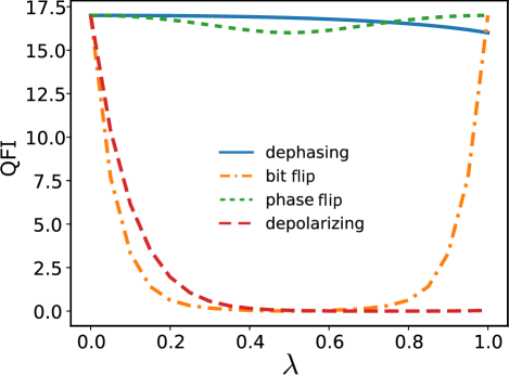
Figure 7: QFI under different noises.

Appendix D Noisy QFI of graph states

In this appendix, we examine how different types of noise impact the QFI. In addition to dephasing, we also encounter bit flip, phase flip, and depolarizing. The relevant Kraus operators are as follows:

$K_{0}=\sqrt{1-\gamma}\begin{pmatrix}1&0\\ 0&1\end{pmatrix};K_{1}=\sqrt{\gamma}\begin{pmatrix}0&1\\ 1&0\end{pmatrix},\text{ for bit flip},$ $K_{0}=\sqrt{1-\gamma}\begin{pmatrix}1&0\\ 0&1\end{pmatrix};K_{1}=\sqrt{\gamma}\begin{pmatrix}1&0\\ 0&-1\end{pmatrix},\text{ for phase flip},$ $K_{0}=\sqrt{1-\gamma}\begin{pmatrix}1&0\\ 0&1\end{pmatrix};K_{1}=\sqrt{\gamma/3}\begin{pmatrix}0&1\\ 1&0\end{pmatrix};K_{2}=\sqrt{\gamma/3}\begin{pmatrix}0&-i\\ i&0\end{pmatrix};K_{3}=\sqrt{\gamma/3}\begin{pmatrix}1&0\\ 0&-1\end{pmatrix},\text{ for depolarizing},$ where $\gamma\in[0,1]$ the noise probability. The QFI is shown in Fig. 7, with different noises.

Appendix E Bayes Inference

We start from the final state

$$\rho_{N}(\phi)=\dfrac{1}{2^{N}}\Big{(}I^{\otimes N}+\sin(\phi)\sin[(N-1)\phi]\sigma_{z}^{\otimes N}\Big{)},$$ (E.1)

when $\lambda=1$. Because $\sigma_{z}^{\otimes N}$ has the same numbers of component $+1$ and $-1$, the state would contain the same number of components $1+\sin(\phi)\sin[(N-1)\phi]$ and $1-\sin(\phi)\sin[(N-1)\phi]$ on the diagonal. Therefore

$$P(D|\phi) =\prod_{k=1}^{2^{N}}{\rm Tr}\Big{[}\rho_{N}(\phi)|k\rangle\langle k|\Big{]}$$

$$=\frac{1}{2^{N\cdot(2^{N})}}\Bigg{[}(1+\sin(\phi)\sin[(N-1)\phi])^{2^{(N-1)}}(1-\sin(\phi)\sin[(N-1)\phi])^{2^{(N-1)}}\Bigg{]}$$

$$=\frac{1}{2^{N\cdot(2^{N})}}\Bigg{[}1-\sin^{2}(\phi)\sin^{2}[(N-1)\phi]\Bigg{]}^{2^{(N-1)}}$$

$$=\frac{1}{2^{N\cdot(2^{N})}}\sum_{k=0}^{2^{N-1}}\binom{2^{N-1}}{k}(-1)^{k}\sin^{2k}(\phi)\sin^{2k}[(N-1)\phi],$$ (E.2)

And then $P(\phi|D)$ is

$$P(\phi|D)=\int P(D|\phi)d\phi =\frac{1}{2^{N\cdot(2^{N})}}\int\sum_{k=0}^{2^{N-1}}\binom{2^{N-1}}{k}(-1)^{k}\sin^{2k}(\phi)\sin^{2k}[(N-1)\phi]d\phi$$

$$=\frac{1}{2^{N\cdot(2^{N})}}\sum_{k=0}^{2^{N-1}}\binom{2^{N-1}}{k}(-1)^{k}\int\sin^{2k}(\phi)\sin^{2k}[(N-1)\phi]d\phi.$$ (E.3)

Finally, we obtain

$$\phi_{\rm estimated}=\int\phi P(\phi|D)d\phi.$$ (E.4)

The integrals in Eqs. (E, E.4) are derived numerically.

Data availability

Data are available from the corresponding authors upon reasonable request.

Code availability

All codes used to produce the findings of this study are incorporated into tqix Viet et al. (2023); Ho et al. (2021) and available at: https://github.com/echkon/tqix-developers.

Author contributions statement

P.T.N and T.K.L. wrote the initial code and implemented the numerical simulation. L.B.H. derived the theoretical framework, implemented the numerical simulation, and analyzed the results. L.B.H. and H.Q.N supervised the work. All authors discussed and wrote the manuscript.

Competing interests

The author declares no competing interests.

References

- Degen et al. (2017) C. L. Degen, F. Reinhard, and P. Cappellaro, Rev. Mod. Phys. 89, 035002 (2017).
- Chalopin et al. (2018) T. Chalopin, C. Bouazza, A. Evrard, V. Makhalov, D. Dreon, J. Dalibard, L. A. Sidorenkov, and S. Nascimbene, Nature Communications 9, 4955 (2018).
- Pezzè et al. (2018) L. Pezzè, A. Smerzi, M. K. Oberthaler, R. Schmied, and P. Treutlein, Rev. Mod. Phys. 90, 035005 (2018).
- Ho and Kondo (2019) L. B. Ho and Y. Kondo, Physics Letters A 383, 153 (2019).
- Friis et al. (2017) N. Friis, D. Orsucci, M. Skotiniotis, P. Sekatski, V. Dunjko, H. J. Briegel, and W. Dür, New Journal of Physics 19, 063044 (2017).
- Shettell and Markham (2020) N. Shettell and D. Markham, Phys. Rev. Lett. 124, 110502 (2020).
- Wang and Fang (2020) Y. Wang and K. Fang, Phys. Rev. A 102, 052601 (2020).
- Le et al. (2023) T. K. Le, H. Q. Nguyen, and L. B. Ho, Scientific Reports 13, 17775 (2023).
- Niezgoda and Chwedeńczuk (2021) A. Niezgoda and J. Chwedeńczuk, Phys. Rev. Lett. 126, 210506 (2021).
- Chu et al. (2023) Y. Chu, X. Li, and J. Cai, Phys. Rev. Lett. 130, 170801 (2023).
- Avdic et al. (2023) I. Avdic, L. M. Sager-Smith, I. Ghosh, O. C. Wedig, J. S. Higgins, G. S. Engel, and D. A. Mazziotti, Phys. Rev. Res. 5, 043097 (2023).
- Zhang and Duan (2014) Z. Zhang and L. M. Duan, New Journal of Physics 16, 103037 (2014).
- Maccone and Riccardi (2020) L. Maccone and A. Riccardi, Quantum 4, 292 (2020).
- Gessner et al. (2020) M. Gessner, A. Smerzi, and L. Pezzè, Nature Communications 11, 3817 (2020).
- Troullinou et al. (2023) C. Troullinou, V. G. Lucivero, and M. W. Mitchell, Phys. Rev. Lett. 131, 133602 (2023).
- Cimini et al. (2019) V. Cimini, I. Gianani, N. Spagnolo, F. Leccese, F. Sciarrino, and M. Barbieri, Phys. Rev. Lett. 123, 230502 (2019).
- Jung et al. (2021) K. Jung, M. H. Abobeih, J. Yun, G. Kim, H. Oh, A. Henry, T. H. Taminiau, and D. Kim, npj Quantum Information 7, 41 (2021).
- Costa et al. (2021) N. F. Costa, Y. Omar, A. Sultanov, and G. S. Paraoanu, EPJ Quantum Technology 8, 16 (2021).
- Cimini et al. (2023) V. Cimini, M. Valeri, E. Polino, S. Piacentini, F. Ceccarelli, G. Corrielli, N. Spagnolo, R. Osellame, and F. Sciarrino, Advanced Photonics 5, 016005 (2023).
- Rinaldi et al. (2023) E. Rinaldi, M. G. Lastre, S. G. Herreros, S. Ahmed, M. Khanahmadi, F. Nori, and C. S. Muñoz, “Parameter estimation by learning quantum correlations in continuous photon-counting data using neural networks,” (2023), arXiv:2310.02309 [quant-ph] .
- Kessler et al. (2014) E. M. Kessler, I. Lovchinsky, A. O. Sushkov, and M. D. Lukin, Phys. Rev. Lett. 112, 150802 (2014).
- Shettell et al. (2021) N. Shettell, W. J. Munro, D. Markham, and K. Nemoto, New Journal of Physics 23, 043038 (2021).
- Yamamoto et al. (2022) K. Yamamoto, S. Endo, H. Hakoshima, Y. Matsuzaki, and Y. Tokunaga, Phys. Rev. Lett. 129, 250503 (2022).
- Rojkov et al. (2022) I. Rojkov, D. Layden, P. Cappellaro, J. Home, and F. Reiter, Phys. Rev. Lett. 128, 140503 (2022).
- Proctor et al. (2018) T. J. Proctor, P. A. Knott, and J. A. Dunningham, Phys. Rev. Lett. 120, 080501 (2018).
- Rahim et al. (2023) M. T. Rahim, A. Khan, U. Khalid, J. u. Rehman, H. Jung, and H. Shin, Scientific Reports 13, 11630 (2023).
- Koczor et al. (2020) B. Koczor, S. Endo, T. Jones, Y. Matsuzaki, and S. C. Benjamin, New Journal of Physics 22, 083038 (2020).
- Yang et al. (2021) X. Yang, X. Chen, J. Li, X. Peng, and R. Laflamme, Scientific Reports 11, 672 (2021).
- Kaubruegger et al. (2021) R. Kaubruegger, D. V. Vasilyev, M. Schulte, K. Hammerer, and P. Zoller, Phys. Rev. X 11, 041045 (2021).
- Meyer et al. (2021) J. J. Meyer, J. Borregaard, and J. Eisert, npj Quantum Information 7, 89 (2021).
- Marciniak et al. (2022) C. D. Marciniak, T. Feldker, I. Pogorelov, R. Kaubruegger, D. V. Vasilyev, R. van Bijnen, P. Schindler, P. Zoller, R. Blatt, and T. Monz, Nature 603, 604 (2022).
- Kaubruegger et al. (2023) R. Kaubruegger, A. Shankar, D. V. Vasilyev, and P. Zoller, PRX Quantum 4, 020333 (2023).
- Portolés et al. (2022) E. Portolés, S. Iwakiri, G. Zheng, P. Rickhaus, T. Taniguchi, K. Watanabe, T. Ihn, K. Ensslin, and F. K. de Vries, Nature Nanotechnology 17, 1159 (2022).
- Gulka et al. (2021) M. Gulka, D. Wirtitsch, V. Ivády, J. Vodnik, J. Hruby, G. Magchiels, E. Bourgeois, A. Gali, M. Trupke, and M. Nesladek, Nature Communications 12, 4421 (2021).
- Carmiggelt et al. (2023) J. J. Carmiggelt, I. Bertelli, R. W. Mulder, A. Teepe, M. Elyasi, B. G. Simon, G. E. W. Bauer, Y. M. Blanter, and T. van der Sar, Nature Communications 14, 490 (2023).
- Huxter et al. (2022) W. S. Huxter, M. L. Palm, M. L. Davis, P. Welter, C.-H. Lambert, M. Trassin, and C. L. Degen, Nature Communications 13, 3761 (2022).
- Sahin et al. (2022) O. Sahin, E. de Leon Sanchez, S. Conti, A. Akkiraju, P. Reshetikhin, E. Druga, A. Aggarwal, B. Gilbert, S. Bhave, and A. Ajoy, Nature Communications 13, 5486 (2022).
- Garrido Alzar (2019) C. L. Garrido Alzar, AVS Quantum Science 1, 014702 (2019), https://pubs.aip.org/avs/aqs/article-pdf/doi/10.1116/1.5120348/14571801/014702_1_online.pdf .
- Kumar et al. (2022) P. Kumar, F. Fabre, A. Durand, T. Clua-Provost, J. Li, J. Edgar, N. Rougemaille, J. Coraux, X. Marie, P. Renucci, C. Robert, I. Robert-Philip, B. Gil, G. Cassabois, A. Finco, and V. Jacques, Phys. Rev. Appl. 18, L061002 (2022).
- Hein et al. (2006) M. Hein, W. Dür, J. Eisert, R. Raussendorf, M. V. den Nest, and H.-J. Briegel, “Entanglement in graph states and its applications,” in Proceedings of the International School of Physics ”Enrico Fermi”, Ebook Volume 162: Quantum Computers, Algorithms and Chaos (IOS Press, 2006) pp. 115–218.
- Hein et al. (2004) M. Hein, J. Eisert, and H. J. Briegel, Phys. Rev. A 69, 062311 (2004).
- Bell et al. (2014a) B. A. Bell, D. A. Herrera-Martí, M. S. Tame, D. Markham, W. J. Wadsworth, and J. G. Rarity, Nature Communications 5, 3658 (2014a).
- Schlingemann and Werner (2001) D. Schlingemann and R. F. Werner, Phys. Rev. A 65, 012308 (2001).
- Bell et al. (2014b) B. A. Bell, D. Markham, D. A. Herrera-Martí, A. Marin, W. J. Wadsworth, J. G. Rarity, and M. S. Tame, Nature Communications 5, 5480 (2014b).
- Pezzé and Smerzi (2009) L. Pezzé and A. Smerzi, Phys. Rev. Lett. 102, 100401 (2009).
- Giovannetti et al. (2004) V. Giovannetti, S. Lloyd, and L. Maccone, Science 306, 1330 (2004), https://www.science.org/doi/pdf/10.1126/science.1104149 .
- Giovannetti et al. (2006) V. Giovannetti, S. Lloyd, and L. Maccone, Phys. Rev. Lett. 96, 010401 (2006).
- Huelga et al. (1997) S. F. Huelga, C. Macchiavello, T. Pellizzari, A. K. Ekert, M. B. Plenio, and J. I. Cirac, Phys. Rev. Lett. 79, 3865 (1997).
- Smirne et al. (2016) A. Smirne, J. Kołodyński, S. F. Huelga, and R. Demkowicz-Dobrzański, Phys. Rev. Lett. 116, 120801 (2016).
- Matsuzaki et al. (2011) Y. Matsuzaki, S. C. Benjamin, and J. Fitzsimons, Phys. Rev. A 84, 012103 (2011).
- Chin et al. (2012) A. W. Chin, S. F. Huelga, and M. B. Plenio, Phys. Rev. Lett. 109, 233601 (2012).
- Tanaka et al. (2015) T. Tanaka, P. Knott, Y. Matsuzaki, S. Dooley, H. Yamaguchi, W. J. Munro, and S. Saito, Phys. Rev. Lett. 115, 170801 (2015).
- Ho et al. (2020) L. B. Ho, H. Hakoshima, Y. Matsuzaki, M. Matsuzaki, and Y. Kondo, Phys. Rev. A 102, 022602 (2020).
- Tekely (2002) P. Tekely, Magnetic Resonance in Chemistry 40, 800 (2002).
- PARIS (2009) M. G. A. PARIS, International Journal of Quantum Information 07, 125 (2009), https://doi.org/10.1142/S0219749909004839 .
- Dür et al. (2003) W. Dür, H. Aschauer, and H.-J. Briegel, Phys. Rev. Lett. 91, 107903 (2003).
- Uhlenbeck and Ornstein (1930) G. E. Uhlenbeck and L. S. Ornstein, Phys. Rev. 36, 823 (1930).
- Yu and Eberly (2010) T. Yu and J. Eberly, Optics Communications 283, 676 (2010), quo vadis Quantum Optics?
- Thomas et al. (2022) P. Thomas, L. Ruscio, O. Morin, and G. Rempe, Nature 608, 677–681 (2022).
- Vigliar et al. (2021) C. Vigliar, S. Paesani, Y. Ding, J. C. Adcock, J. Wang, S. Morley-Short, D. Bacco, L. K. Oxenløwe, M. G. Thompson, J. G. Rarity, and A. Laing, Nature Physics 17, 1137–1143 (2021).
- Ho (2023) L. B. Ho, EPJ Quantum Technology 10, 37 (2023).
- Wilcox (2004) R. M. Wilcox, Journal of Mathematical Physics 8, 962 (2004), https://pubs.aip.org/aip/jmp/article-pdf/8/4/962/7440792/962_1_online.pdf .
- Viet et al. (2023) N. T. Viet, N. T. Chuong, V. T. N. Huyen, and L. B. Ho, Computer Physics Communications 286, 108686 (2023).
- Ho et al. (2021) L. B. Ho, K. Q. Tuan, and H. Q. Nguyen, Computer Physics Communications 263, 107902 (2021).