Reasoning with the Theory of Mind for Pragmatic Semantic Communication

Abstract

In this paper, a pragmatic semantic communication framework that enables effective goal-oriented information sharing between two-intelligent agents is proposed. In particular, semantics is defined as the causal state that encapsulates the fundamental causal relationships and dependencies among different features extracted from data. The proposed framework leverages the emerging concept in machine learning (ML) called theory of mind (ToM). It employs a dynamic two-level (wireless and semantic) feedback mechanism to continuously fine-tune neural network components at the transmitter. Thanks to the ToM, the transmitter mimics the actual mental state of the receiver’s reasoning neural network operating semantic interpretation. Then, the estimated mental state at the receiver is dynamically updated thanks to the proposed dynamic two-level feedback mechanism. At the lower level, conventional channel quality metrics are used to optimize the channel encoding process based on the wireless communication channel’s quality, ensuring an efficient mapping of semantic representations to a finite constellation. Additionally, a semantic feedback level is introduced, providing information on the receiver’s perceived semantic effectiveness with minimal overhead. Numerical evaluations demonstrate the framework’s ability to achieve efficient communication with a reduced amount of bits while maintaining the same semantics, outperforming conventional systems that do not exploit the ToM-based reasoning.

I Introduction

Future 6G wireless systems will transmit and process large volume of data potentially under stringent requirements of ultra-low latency, ultra-reliability and high throughput, to support new connected intelligence (CI) applications such as haptics, brain-computer interaction, flying vehicles, extended reality (XR), and the metaverse [1]. 6G systems could transmit only essential information relevant to the end-user to meet this need for high-rate, high-reliability, and time-criticality for the aforementioned CI applications, . This concept forms the basis of semantic communication (SC) systems [2, 3, 4].

Despite a recent surge in SC research [5, 6], focus has been mainly on potential SC gains assuming an error-free SC channel. Nevertheless, no channel is error-free. With SC, the communication channel has two components: wireless and semantic. One critical challenge that often goes unnoticed is the need to dynamically adapt transmission strategies at the semantic level based on end-to-end performance. The evaluation of errors at the semantic channel was provided by [7] for the first time, showing that the semantic channel’s quality critically impacts the overall communication performance. In wireless communication, adaptive mechanisms adjust transceiver design based on estimated link quality for a trade-off between robustness and efficiency. This paper asserts the need for adaptive mechanisms at the semantic level as well [8]. This requires at the system architecture level the introduction of a semantic plane [9] where feedback information from the semantic receiver to the semantic transmitter can be exchanged over a dedicated plane. The adaptation of semantic encoder and decoder should be driven by the receiver’s performance in reconstructing semantic information, ensuring optimized communication and improved overall system efficiency. By addressing these challenges, we can pave the way for the successful integration of SC systems into existing digital communication infrastructure, with minimal changes to existing layered architecture. However, many existing works [5, 7, 6] 1) fix the parameters of transmitter and receiver neural network (NN) components during offline training and, 2) NN’s parameters are jointly learned to minimize semantic reconstruction errors. This approach is often adopted due to the increased complexity and re-training overhead to update the parameters via online learning. The training aims to minimize semantic reconstruction errors while maximizing a performance target such as semantic compression gain. Nevertheless, such approach to training does not guarantee expected semantic reliability [10] in dynamic communication scenarios where environment variations or task’s specifications changes may occur. Herein, a key concern arises: how should the semantic design components be adjusted to avoid or rectify errors at the semantic level in subsequent transmissions if the receiver cannot decode the information reliably? This question draws parallels to the concept of automatic repeat request (ARQ) used in traditional systems where a feedback control channel is used to inform on the positive or negative acknowledgement on received information. In an SC system, transmitters and receivers must extract (at the transmitter) and interpret (at the receiver) semantic messages based on different beliefs and knowledge. Such mismatch on logic and reasoning states at transmitter and receiver can cause critical errors, which most of the time are undetected and thus systematically repeated.

We propose harnessing the idea of “theory of mind” (ToM) [11] to tackle these challenges by operating before communication at the transmitter an estimate of the mental state of the receiver (a priori knowledge and believes). Thanks to such a pragmatic communication approach, we contribute to improving the overall SC communication accuracy, reliability, and reduction of needed communication and processing resources.

I-A Contributions

Our framework considers the semantic information present in the data to be the causal state extracted using graph NNs (GNN) [12] from observed time series data at the transmitter. We chose GNN since it provides a rigorous framework to extract the causal relations present among the features in the data as a directed acyclic graph. By leveraging ToM, we can dynamically adapt the parameters of NNs based on feedback measures of semantic effectiveness. This approach enables effective semantic design component adjustment, improving subsequent transmissions’ reliability and performance in SC systems. Additionally, to accurately reason about other nodes, we introduce a two-level feedback mechanism. The first level involves a semantic level of feedback, enabling dynamic adjustments to the semantic representation component and causal state extraction. The second level consists of conventional channel quality feedback, used to optimize the design of the constellation-constrained channel input. Finally, we demonstrate via simulations the superior spectral efficiency of the proposed ToM-based SC system compared to conventional schemes such as repetition coding and HARQ applied to SC systems. Additionally, we demonstrated that the proposed SC system requires fewer redundant semantic symbols to be transmitted in order to achieve close to perfect semantic reliability. This is in contrast to the state-of-the-art systems that do not employ ToM reasoning.

II System Model

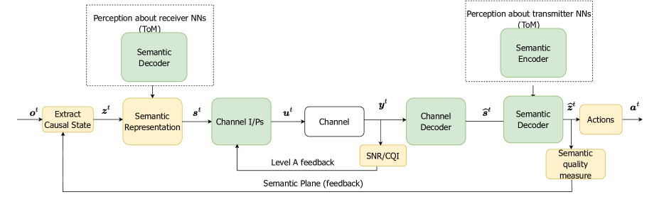
Figure 1: Proposed system model.

$$\vspace{-0mm}\begin{array}[]{l}C_{t}({\bm{s}}^{t},\widehat{{\bm{s}}}^{t})=\textrm{KLD}\left(\pi({\bm{a}}^{t}\mid\bm{z}^{t})\,\mid\mid\,\sum\limits_{{\bm{y}}^{t},\bm{u}^{t},\widehat{{\bm{s}}}^{t}}p({{\bm{y}}}^{t}\mid{\bm{u}}^{t})p(\widehat{{\bm{s}}}^{t}\mid{\bm{y}}^{t})p(\widehat{\bm{z}}^{t}\mid{{\bm{s}}}^{t})\pi({\bm{a}}^{t}\mid\widehat{\bm{z}}^{t})\right).\end{array}\vspace{-3mm}$$ (1)

We consider the SC system shown in Fig. 1. In this system, a transmitter has access to a sequence of observations represented as a time series data, where each $N-$dimensional vector of observations ${\bm{o}}^{t}$ belongs to a set $\mathcal{O}$. The transmitter’s goal is to transmit a concise description, $\bm{z}^{t}$, of the data ${\bm{o}}^{t}$ that can be efficiently interpreted at the receiver. This description captures the semantic information of the data, including the intrinsic causal relationships [2]. The receiver aims to use the reconstructed received messages $\widehat{\bm{z}}^{t}$ to perform a set of actions ${\bm{a}}^{t}\in\mathcal{A}$, sampled using the distribution $\pi({\bm{a}}^{t}\mid\widehat{\bm{z}}^{t})$. Contrary to previous works [5], we constrain the channel input to a finite constellation. As such, the channel inputs $\bm{u}^{t}$ are selected from a digital modulation scheme of order $M$, where the constellation symbols are represented by $\mathcal{M}=\{c_{1},\cdots,c_{M}\}$. Consequently, the channel input $\bm{u}^{t}$ is a digital sequence of varying dimension (that gets learned), with each element drawn from the constellation symbols $\mathcal{M}$. Hence, we refer to this sequence as a constellation symbol sequence.

The primary innovation that distinguishes this paper from the state-of-the-art [5, 7, 6] is the incorporation of receiver feedback, denoted as $d^{t}\in\mathcal{D}$ (a scalar value), through a feedback channel called the “semantic plane.” The set $\mathcal{D}$ here represents the semantic effectiveness measure. Semantic effectiveness captures the accuracy of the actions performed at the receiver using the reconstructed semantic state $\widehat{\bm{z}}^{t}$. In particular, to capture the semantic effectiveness, we introduce the metric $C_{t}$, which captures the causal impact of the transmitted message (via the receiver’s actions) as observed through a channel with a response characterized using $p({\bm{y}}^{t}\mid\bm{u}^{t})$ (this distribution could capture the fading and interference in the wireless environment). In other words, $C_{t}$ measures the semantic effectiveness (inversely proportional to $C_{t}$) of the transmitted message to the end-user and is written as (1), where $\textrm{KLD}(p\mid\mid q)$ represents the KL divergence between $p$ and $q$. Hence, the feedback $d^{t}$ gives the transmitter an indication of whether those are accurate in terms of achieving the system’s long term goal. The transmitter can adjust its transmission strategy and update its causal reasoning components by using the feedback received through the semantic plane. This dynamic nature of our proposed method ensures that the NN components are continuously updated based on the real-time feedback from the receiver. As a result, the system can adapt and optimize its performance dynamically during communication, leading to more efficient and effective semantic communication. We also consider a second level of feedback through classical measures like the signal-to-noise-ratio (SNR) or the channel quality indicator (CQI) measure, defined as $p^{t}$, which gets used by the channel encoder to dynamically adjust its constellation sequence.

As an illustrative example of the proposed system, we consider a variant of the problem of rendezvous between two robots exploring an unknown environment [13]. That is, how can two autonomous exploring agents that can communicate with one another over long distances meet if they start exploring at different locations in an unknown environment. The intended application is collaborative map exploration. Herein, we can consider the case in which only one of the robot, say $A$ has the necessary sensing modalities to detect the landmarks near it. Robot $A$ communicates this information to robot $B$, which receives it over a wireless channel. Moreover, utilizing the extracted information, $B$ attempts to make additional movements along the trail and feedback its actions back to robot $A$. Next, we define the causal generative model that describes the data generation and transmission signal.

II-A Causal discovery model

The causal relationships present within the source data can be represented as a causal graph, and the process of learning this graph is referred to as the causal discovery problem [14]. In a complex environment with high-dimensional observations, such as images or video, learning a compact latent state space that captures the causal dynamics of the environment has been shown to be more computationally efficient than learning predictions directly in the observation space [15]. This latent space, denoted ${\bm{s}}^{t}$ is the semantic representation here. The generative model for a dataset of observations and transmitter actions ($\bm{u}^{t}$), represented as $({\bm{o}}^{0:T},\bm{u}^{0:T})$, can be formulated as follows ($\bm{\theta}$ is the set of the NN parameters):

$$p({\bm{o}}^{0:T},\bm{u}^{0:T})= \int\prod\limits_{t}p_{\bm{\theta}}({\bm{o}}^{t}\mid\bm{z}^{t})p_{\bm{\theta}}(\bm{z}^{t}\mid\bm{z}^{t-1},d^{t-1})$$ (2)

$$\pi_{\bm{\theta}}({\bm{s}}^{t}\mid\bm{z}^{t})d\pi_{\bm{\theta}}(\bm{u}^{t}\mid\bm{z}^{t},p^{t-1})d\bm{z}^{0:T}d{\bm{s}}^{0:T},$$

where $p_{\bm{\theta}}({\bm{o}}^{t}\mid\bm{z}^{t})$ and $p_{\bm{\theta}}(\bm{z}^{t}\mid\bm{z}^{t-1},d^{t-1})$ are the observation model and the causal transition model, respectively. The causal structure $\bm{z}^{t}$ is represented as a sequence of entities (scalar variables present in ${\bm{o}}^{t}$) and their relations. While extracting the causal structure, any variables in ${\bm{o}}^{t}$ that remain unconnected in the graph can be considered irrelevant and will not be transmitted. As mentioned in previous studies [10, 16], acquiring causal representations can result in AI solutions that exhibit distribution invariance, enabling adaptability across various interventional distributions. In this paper, we opted not to delve into discussions about interventions as they have already been addressed in our previous work [10]. From SC perspective, this implies constructing solutions with reduced training overhead, leading to improved real-time decision-making capabilities compared to data-intensive AI approaches. It is important to note that none of the factors in equation (2) are known and must be learned from the data. The feedback of the receiver actions $d^{t}$ is reflected in the transmitter policy $\pi_{\bm{\theta}}({\bm{s}}^{t}\mid\bm{z}^{t})$ that chooses the transmitted semantic representation, at time $t$. The design of the representation ${\bm{s}}^{t}$ relies on the specific semantic information intended to be conveyed, which, in turn, is influenced by the receiver’s actions. Hence, we next define the semantic information $\mathbb{S}_{t}$, essential for the subsequent problem formulations.

II-B Semantic information measure

Using the novel semantic information measures in [10], we directly obtain the transmitted and received semantic information as follows. We omit the time superscript for convenience.

Lemma 1.

The semantic information conveyed by any causal state $\bm{z}\in\mathcal{C}_{1}$ can be written as the average across the information carried by the possible actions (${\bm{a}}$) that follow from $\bm{z}$. Further, mathematically, we can write the semantic information conveyed by $\bm{z}$ as

$$\vspace{-2mm}\mathbb{S}(\bm{z})=\sum\limits_{{\bm{a}}\in\mathcal{A}}\pi({\bm{a}}\mid\bm{z})\log\frac{\pi({\bm{a}}\mid\bm{z})}{\pi({\bm{a}})}=\textrm{KL}(\pi({\bm{a}}\mid\bm{z})\mid\mid\pi({\bm{a}})).$$ (3)

Leveraging [10, Corollary 1], we obtain the average semantic information extracted by the receiver as (5). $Z_{\widehat{\bm{z}}_{t}\bm{z}_{t}}$ is the semantic similarity between the transmitted and reconstructed causal states, which is defined in [10, Corollary 1].

$$\mathbb{E}_{\bm{u}_{t}}\left[S_{r,t}(\widehat{\bm{z}}_{k,t};\bm{u}_{k,t}\mid l_{k,t},[\widehat{\bm{z}}_{k,t-1}],\pi_{l,t})\right] =$$ (4)

$$\sum\limits_{\bm{u}_{t},{\bm{y}}_{k,t}}\!\!\!\!\pi\left(\bm{u}_{k,t}\mid[\bm{z}_{t}]\right)S({\bm{z}}_{t}\mid[\bm{z}_{t-1}])p({\bm{y}}_{t}\mid\bm{u}_{t})\left[\sum\limits_{\widehat{\bm{z}}_{t}}\pi_{\bm{z}_{t}}\log\frac{\pi_{\bm{z}_{t}}}{\pi(\widehat{\bm{z}}_{t}\mid\widehat{\bm{z}}_{t-1}])}Z_{\widehat{\bm{z}}_{t}\bm{z}_{t}}\right].$$ (5)

II-C Semantic reliability

Semantic reliability is quantified by the expression, $p\left(E_{t}\left({\bm{z}}^{t},{\widehat{\bm{z}}}^{t}\right)<\delta\right)\geq 1-\epsilon,$ where $E_{t}(\bm{z}^{t},{\widehat{\bm{z}}}^{t})=\left\lVert\bm{z}^{t}-\widehat{\bm{z}}^{t}\right\rVert^{2}$ represents semantic distortion and $\epsilon$ is arbitrarily small. This definition follows our previous works [10, 16]. This metric reflects the receiver’s ability to reliably reconstruct all the causal aspects in the decoded causal structure. Unlike classical reliability measures, in semantics, we can recover the actual meaning of transmitted messages even with a higher bit error rate (BER), as long as the semantic distortion remains within the set limit. This is illustrated by the choice of $\delta$ here, which depends on the concept of semantic space. The semantic space $\mathcal{K}$ is defined as an $N$-dimensional topological ball centered at the actual state $\bm{z}^{t}$, where all points inside the ball corresponding to the same semantic information. Formally, we can express this as $E_{t}(\bm{z}^{t},{\widehat{\bm{z}}}^{t})\leq\delta$ such that $\mathbb{I}_{\phi}(\bm{z}^{t})=\mathbb{I}_{\phi}(\widehat{\bm{z}}^{t})$, where $E_{t}$ is the topological distance between states $\bm{z}^{t}$ and $\widehat{\bm{z}}^{t}$, $\delta$ is the radius of the topological ball, and $\mathbb{I}_{\phi}$ is a mapping function that maps states to their corresponding semantic information.

Having defined the necessary metrics, we next formulate the problem for the transmitter and receiver components in our SC system.

III Theory of Mind based SC Design

Here, we first discuss the causal discovery component at the transmit side, that represents the mapping from ${\bm{o}}^{t}$ to $\bm{z}^{t}$.

III-A Causal discovery at the transmitter

The fundamental assumption underlying causal discovery here is that there exists a fixed function ${\bm{g}}$ that characterizes the dynamics of all samples ${\bm{o}}^{t}\in\mathcal{O}$, given their past observations up to time $t$ and the underlying causal graph $\mathcal{G}$. This can be written using the Granger causality concept [17] as follows:

$${\bm{o}}^{t+1}={\bm{g}}({\bm{o}}^{\leq t},\mathcal{G})+{\bm{n}}^{t+1}.$$ (6)

In this data-generating process, we model two variables: the causal graph $\mathcal{G}$, and the dynamics ${\bm{g}}$, which are shared across all samples. By separating the causal graph from the dynamics, we can design our model accordingly. Specifically, we introduce a causal discovery encoder $f_{\bm{\theta}}$, which learns to infer the causal graph $\mathcal{G}$ given the sample ${\bm{o}}^{t}$. $\bm{\theta}$ represents the NN parameters. Additionally, we introduce a dynamics decoder ${\bm{g}}_{\theta}$ that learns to approximate the dynamics ${\bm{g}}$. This division of the model allows us to effectively capture the relationship between the causal graph and the shared dynamics within the data.

III-A1 Problem formulation

To approach the problem of causal discovery, we adopt a probabilistic framework and model the functions $f_{\bm{\theta}}$ and $g_{\theta}$ using variational inference. We choose the encoder $f_{\bm{\theta}}$ by incorporating an encoding function $q_{\bm{\theta}}(\bm{z}\mid{\bm{o}})$, which produces a distribution over $\bm{z}$ that represents the predicted edges $\mathcal{E}^{\text{Enc}}$ in the causal graph. Simultaneously, we train a decoder $p_{\theta}({\bm{o}}\mid\bm{z})$ that probabilistically captures the dynamics of the time-series based on the predicted causal relationships.

In our framework, we select the negative log-likelihood as the loss function $\mathcal{V}_{f}$ for the decoder. Additionally, we incorporate a regularizer that measures the Kullback-Leibler divergence (KLD) to a prior distribution over $G$. This regularizer encourages the model to learn causal structures consistent with our prior knowledge. Overall, our loss function $\mathcal{V}_{f}$ represents a variational lower bound [18]:

$$\mathcal{V}_{f}=\mathbb{E}_{q_{\phi}(\bm{z}\mid{\bm{o}})}\log p_{\theta}({\bm{o}}\mid\bm{z})-\textrm{KL}(q_{\phi}(\bm{z}\mid{\bm{x}})\mid\mid p(\bm{z})).$$ (7)

Further, we formally write the causal discovery problem as (with variables $x^{*}$ representing the optimized quantities):

$$\left[\mathcal{G}^{*},\bm{z}_{t}^{*}\right]=\operatorname*{arg\,min}\limits_{\mathcal{G}}-\mathcal{V}_{f}.$$ (8)

III-A2 Causal discovery solution

To optimize (7), The encoder $q_{\bm{\theta}}(\bm{z}\mid{\bm{o}})$ is designed as a GNN [12], denoted as $f_{\text{enc},{\bm{\theta}}}$. The output $z_{ij}$ of the encoder represents the predicted edges $\mathcal{E}^{enc}$ in the causal graph $\mathcal{G}$. The decoder $p_{\theta}({\bm{o}}\mid\bm{z})$ captures the dynamics of the time-series data based on the predicted causal relations. It takes into account both the predicted causal relations $z_{ij}$ and ${\bm{o}}^{t}$ as its input. First, it propagates information along the predicted edges by applying a NN $f_{e}$, and compute $h_{ij}^{t}=\sum\limits_{e>0}z_{ij,e}f_{e}([o_{i}^{t},o_{j}^{t}])$. Then, the decoder accumulates the incoming messages to each node and applies a NN $f_{v}$ to predict the change between the current and the next time-step:

$$\begin{array}[]{l}\mu_{j}^{t+1}=o_{j}^{t}+f_{v}(\sum_{i\neq j}h_{ij}^{t}o_{j}^{t})\\ p_{\theta}(o_{j}^{t+1}\mid{\bm{o}}^{t},\bm{z})=\mathcal{N}(\mu_{j}^{t+1},\sigma^{2}).\end{array}$$ (9)

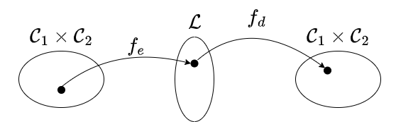
Figure 2: A semantic decoder function maps points in $\mathcal{C}_{1}\times\mathcal{C}_{2}$ to $\mathcal{C}_{1}\times\mathcal{C}_{2}$ via $\mathcal{L}$ (the semantic language), where $f_{e}$ is the encoder function and $f_{d}$ the decoder function.

Having discussed the causal discovery problem, we next move on to computing the semantic representation ${\bm{s}}^{t}$.

III-B Theory of mind based semantic representation

Communication is successful when the concept defined as $\bm{z}^{t}\in\mathcal{C}_{1}$ is perceived correctly by the receiver. This means that the extracted causal state at the receiver, $\widehat{\bm{z}}^{t}\in\mathcal{C}_{2}$ is such that it belongs to the semantic space (defined as the Euclidean space over which the semantic information conveyed by $\widehat{\bm{z}}$ is the same within a ball of radius $\delta$) [10]. $\mathcal{C}_{i}$ represents the conceptual space that includes the set of all possible meanings or structure present in the data [19]. The decoded state description at the listener, constrained to a semantic message space (represented as $\mathcal{S}_{z^{t}}$ corresponding to message $\bm{z}^{t}$), can convey the same semantic content (defined $S_{z^{t}}$). As a result, they are considered semantically similar. Hence, we can achieve the same semantic reliability. This semantic message space corresponding to $\widehat{\bm{z}}^{t}$ can be described as

$$\vspace{-1mm}E(\bm{z}^{t},{\widehat{\bm{z}}}^{t})\leq\delta,\,\,\mbox{s.t.}\,\,E({\mathbb{S}}_{t},{\widehat{\mathbb{S}}}_{t})=0,\vspace{-0mm}$$ (10)

where $E({\bm{x}},\widehat{{\bm{x}}})=\left\lVert{\bm{x}}-\widehat{{\bm{x}}}\right\rVert^{2}$. $\mathbb{S}_{t}$ denotes the semantic information conveyed by $\bm{z}^{t}$. From an SC point of view (see Fig. 2), the aim is to ensure that the pair of state descriptions $(\bm{z}^{t},\widehat{\bm{z}}^{t})\in\mathcal{C}_{1}\times\mathcal{C}_{2}$ satisfy the following conditions that represent a meeting of minds between transmitter and receiver,

$$\mathcal{L}(\bm{z}^{t},\widehat{\bm{z}}^{t})=(\bm{z}^{t},\widehat{\bm{z}}^{t}).$$ (11)

The language represented by $\mathcal{L}$ is a cascade of two functions, $\mathcal{L}=f_{d}\circ f_{e}$, where 1) the encoder function $f_{e}$ defined as ${\bm{s}}^{t\,*}=\operatorname*{arg\,max}\limits_{{\bm{s}}^{t}}\pi_{\bm{\theta}}({\bm{s}}^{t}\mid\bm{z}^{t},d^{t-1})$, and 2) the decoder function $f_{d}$ defined as $\widehat{\bm{z}}^{t\,*}=\operatorname*{arg\,max}\limits_{\bm{z}^{t}}p_{\bm{\phi}}(\bm{z}^{t}\mid\widehat{{\bm{s}}}^{t})$. Further, we make the following assumption on the transmitted symbol.

Assumption 1.

For every state description $\bm{z}^{t}$, extracted at time $t$, only one semantic symbol vector ${\bm{s}}^{t}$ is computed. Further, the feedback ($d^{t}$) about the actions executed at the receiver decide the future semantic states to be transmitted (indirectly represent retransmissions at the semantic level).

The semantic level of feedback $d^{t}$ serves as an indicator of the system’s overall performance, encompassing end-to-end aspects. By incorporating the semantic level of feedback, the requirement for multiple layers of feedback found in conventional digital communication systems can be mitigated, reducing control information overhead.

III-B1 Problem formulation at the transmitter

Given the causal state $\bm{z}^{t}$, we further discuss how to compute the mapping from $\bm{z}^{t}$ to the semantic symbol ${\bm{s}}^{t}$. Here, we assume that transmitter states can be decomposed into physical states and private receiver states, namely, $\widetilde{\mathcal{Z}}_{s}=\mathcal{C}_{1}\times\Omega_{r}$, where $\mathcal{C}_{1}$ is the transmitter state space ($\bm{z}^{t}$ belongs here), $\Omega_{r}$ is the receiver’s NN parameter space. Each element part of $\Omega_{r}$ is denoted as $\bm{\omega}_{r,i}$. For transmitter, it performs according to its value function, $Q_{s}:\widetilde{\mathcal{Z}}_{s}\times\mathcal{A}_{s}\rightarrow\mathcal{R}$, where $\mathcal{A}_{s}$ represents the action space (the semantic symbol set for transmitter). We can define the value of a state as $V^{\pi}({\bm{s}}^{t})=\mathbb{E}_{{\bm{s}}^{t},d^{t+1},\cdots}\sum\limits_{t}\gamma^{t}r(d^{t},{\bm{s}}^{t})$, where $d^{t}=\frac{1}{1+C_{t}({\bm{s}}^{t},\widehat{{\bm{s}}}^{t})}$, and $r(d^{t},{\bm{s}}^{t})$ is the reward obtained upon performing the control actions ${\bm{a}}^{t}$ by the receiver. Here, the semantic effectiveness measure fed back from the receiver represents the state transitions akin to reinforcement learning (RL). Further, we can also define the Q-function as $Q_{s}(d^{t},{\bm{s}}^{t})=r(d^{t},{\bm{s}}^{t})+\gamma\mathbb{E}_{d^{t+1}\sim p(d^{t+1}\mid d^{t},{\bm{s}}^{t})}\left[V^{\pi}({\bm{s}}^{t+1})\right]$. We define $\tau_{s}$ as transmitter’s observation and action history $\{d^{0},{\bm{s}}^{0},\cdots,d^{t},{\bm{s}}^{t}\}$. The transmitter estimates a belief about the receiver’s knowledge of the transmitted message (obtained through the respective NN parameters) and their private states. The transmitter must maintain a belief about the private state of receiver, denoted as $b_{s}^{t}(\bm{\omega}_{r,i})$. The transmitter policy averaged over the receiver’s belief distribution will be:

$$\pi_{s}({\bm{s}}^{t}\mid\bm{z}^{t},\bm{\omega}_{s}^{t},\tau_{s}^{t}) =$$ (12)

$$\frac{e^{\left(\beta\sum\limits_{\bm{\omega}_{r,i}\in\Omega_{r}}b_{s}^{t}(\bm{\omega}_{r,i}\mid\tau_{s}^{t})Q_{s}({\bm{s}}^{t},\bm{\omega}_{s},\bm{\omega}_{r,i})\right)}}{\sum\limits_{{\bm{s}}^{t\,\prime}\in\mathcal{S}_{t}}e^{\left(\beta\sum\limits_{\bm{\omega}_{r,i}\in\Omega_{r}}b_{s}^{t}(\bm{\omega}_{r,i}\mid\tau_{s}^{t})Q_{s}({\bm{s}}^{t},\bm{\omega}_{s},\bm{\omega}_{r,i})\right)}},$$

where $\bm{\omega}_{s}$ represents the NN parameters of transmitter. The next challenge lies in how the transmitter can maintain its belief given its observation history. We can utilize counterfactual reasoning in our belief update function [20]. The transmitter traverses all possible private states $\bm{\omega}_{r}$ and estimates how likely the actions it observed are taken given a specific set of private agent states are the correct one. Then, it updates its belief using Bayesian rule:

$$b_{s}^{t}(\bm{\omega}_{r,i}\mid\tau_{s}^{t})=P(\bm{\omega}_{r,i}\mid\tau_{s}^{t},{\bm{a}}^{t})\propto\widehat{\pi}_{r}({\bm{a}}^{t}\mid{\bm{s}}^{t},\bm{\omega}_{r,i})b_{s}^{t-1}(\bm{\omega}_{r,i}),$$ (13)

where $\widehat{\pi}_{r}$ is transmitter’s estimation of receiver policy, learned in centralized training. As per Assumption 1, the transmitter utilizes the fed back actions ${\bm{a}}^{t}$ (denoted $d^{t}$) from the receiver to compute (13). To complete the ToM framework, the transmitter must maintain a belief about the receiver’s private states, and conversely, the receiver must also estimate the transmitter’s state. This is because maintaining accurate beliefs about each other’s private states is crucial for effective coordination among agents. Utilizing the obverter technique [20], we let the transmitter holds a belief $\widehat{b}_{r}$ as the estimation of receiver’s belief about $\bm{\omega}_{s}$ (representing transmitter’s NN parameters). All we need is a belief update function, $f_{r}:\Delta(\Omega_{s})\times\mathcal{A}_{s}\times\widetilde{\mathcal{Z}}_{s}\rightarrow\Delta(\Omega_{s}),$ where $\Delta(\Omega_{s})$ represents a distribution. Belief update function $f_{r}$ takes in the old belief, transmitter’s action, the physical state and returns a new belief as its new estimation of receiver’s belief over $\omega_{s}$. The ability to correctly infer receiver’s private states from their actions and predict others belief about oneself introduces ToM into our agents. Given the semantic representation ${\bm{s}}^{t}$, which is a continuous signal, mapping to the nearest element in the constellation $\mathcal{M}_{t}$ can be computed using a scheme discussed in [21] and is beyond the scope of this paper.

III-B2 Problem formulation for ToM based receiver design

The generative model of the observations and actions sequence at the receiver side can be written as follows:

$$\vspace{-0mm}\begin{array}[]{l}p(\widehat{{\bm{s}}}^{0:T},{\bm{a}}^{0:T})=\\ \int\prod\limits_{t}p_{\bm{\theta}}(\widehat{{\bm{s}}}^{t}\mid\bm{u}^{t})p_{\bm{\theta}}(\bm{z}^{t}\mid\bm{z}^{t-1},\widehat{{\bm{s}}}^{t})\pi_{\bm{\theta}}({\bm{a}}^{t}\mid\bm{z}^{t})d\bm{z}^{0:T},\end{array}\vspace{-0mm}$$ (14)

where we split the observation model, $p_{\bm{\theta}}(\widehat{{\bm{s}}}^{t}\mid\bm{u}^{t})=\int_{{\bm{s}}^{t},\bm{z}^{t}}p_{\bm{\theta}}({\bm{y}}^{t}\mid\bm{u}^{t})p_{\bm{\theta}}(\bm{u}^{t}\mid{\bm{s}}^{t})p_{\bm{\theta}}({\bm{s}}^{t}\mid\bm{z}^{t})p_{\bm{\theta}}({\bm{s}}^{t}\mid\bm{z}^{t})dsdz$. In other words, receiver also learn the transmitter semantic encoder $p_{\bm{\theta}}({\bm{s}}^{t}\mid\bm{z}^{t})$, the channel model $p_{\bm{\theta}}({\bm{y}}^{t}\mid\bm{u}^{t})$ and the channel encoder $p_{\bm{\theta}}(\bm{u}^{t}\mid{\bm{s}}^{t})$. Here one can ask: how does receiver obtain the true transmit signal $\bm{u}^{t}$ to learn channel distribution? We propose that the receiver also have a transmitter model (including the semantic and channel encoders) that generates the transmit signal $\bm{u}^{t}$. Hence, it is essential the receiver’s NN model matches accurately with the transmitter model, if the receiver design can correct the errors in the channel and lead to higher semantic reliability.

Assume that, for every semantic state description, there is an optimal action distribution (receiver policy) from which the actions are sampled. This is represented as $\pi_{\theta}^{*}({\bm{a}}^{t}\mid\widehat{\bm{z}}^{t})$, which represents the implicit semantics that entails from the state description $\bm{z}^{t}$. The cross entropy loss for the pair $(\bm{z}^{t},\widehat{\bm{z}}^{t})$ by using any policy $\pi_{\theta}$ at the receiver can be written as:

$$\mathcal{L}_{CE}(t)=-\sum\limits_{{\bm{a}}^{t}}\pi_{\theta}^{*}\log\pi_{\theta}\vspace{-2mm}$$ (15)

Minimizing $\mathcal{L}_{CE}$ is equivalent to minimizing the KLD between $\pi_{\theta^{\ast}}$ and $\pi_{\theta}$. Here, at the receiver, we assume that, it is aware of the optimal $\pi_{\theta}^{*}({\bm{a}}^{t}\mid\bm{z}^{t})$, which is computed using the transmitter model available at its end. The average cross-entropy loss, which can be interpreted as the semantic effectiveness measure can be written as:

$$\bar{\mathcal{L}}_{CE}(t)=-\sum\limits_{\bm{z}^{t},\widehat{\bm{z}}^{t}}\sum\limits_{{\bm{a}}^{t}}p(\bm{z}^{t},\widehat{\bm{z}}^{t})KLD(\pi_{\theta}^{*}\mid\mid\pi_{\theta}),$$ (16)

where $p(\bm{z}^{t},\widehat{\bm{z}}^{t})=p(\bm{z}^{t})p(\widehat{\bm{z}}^{t}\mid\bm{z}^{t})=p(\bm{z}^{t})\int p(\widehat{\bm{z}}^{t}\mid\widehat{{\bm{s}}}^{t},[\widehat{\bm{z}}^{t-1}])p(\widehat{{\bm{s}}}^{t}\mid\bm{u}^{t})dsdu$.

Now, we have the necessary ingredients to formulate the problem at the receiver side, which can be written as:

$$p(\bm{z}^{t}\mid\widehat{{\bm{s}}}^{t})^{\ast}= \operatorname*{arg\,max}\limits_{p(\bm{z}^{t}\mid\widehat{{\bm{s}}}^{t})}\bar{\mathcal{L}}_{CE}(t)$$ (17)

s.t. $$p\left(E_{t}\left({\bm{z}}^{t},{\widehat{\bm{z}}}^{t}\right)<\delta\right)\geq 1-\epsilon.$$

Further, we obtain the augmented Lagrangian as follows:

$$\mathcal{P}_{2}: \left[p(\bm{z}^{t}\mid\widehat{{\bm{s}}}^{t})^{\ast}\right]$$ (18)

$$=\operatorname*{arg\,max}\limits_{p(\bm{z}^{t}\mid\widehat{{\bm{s}}}^{t})}\bar{\mathcal{L}}_{CE}(t)+\lambda\left(p\left(E_{t}\left({\bm{z}}^{t},{\widehat{\bm{z}}}^{t}\right)<\delta\right)-(1-\epsilon)\right).$$

The Lagrangian in (18) represents the $Q$-function for the receiver side ToM formulation.

Algorithm 1 Proposed Solution for Adaptive ToM Collaboration Emergence

Given: Randomly initialize $\bm{\theta}_{i},\widehat{\bm{\theta}}_{i},\eta_{Q},\eta_{\pi},\eta_{f},i\in\{1,\cdots,N\}$.
Learning rate $\eta$, Batch size $B$

1:for each round do

2:    for $i\in\{s,r\}$ do

3:       Initialize replay buffer $\mathcal{D}\leftarrow\emptyset$

4:       while train agent $i$ do

5:          repeat

6:             Agents sample actions according to equation (12)

7:             Agents update their beliefs

8:             Agents update their estimation of partners’ beliefs

9:          until game ends

10:          Update $\mathcal{D}$ with new trajectory

11:

12:          Sample $B$ trajectories $\{(\omega_{1:N},{\bm{s}}_{0:T},{\bm{a}}_{0:T},r_{0:T})$

13:          $y_{i}^{t,(k)}=r_{i}^{t,(k)}+\gamma\max_{{\bm{s}}\in\mathcal{A}_{s}}Q_{\widehat{\bm{\theta}}_{i}}({\bm{s}},d^{t+1,(k)},\bm{\omega}^{(k)},\widehat{b})$

14:          $L^{Q}=\sum_{t,k}\lvert Q_{\widehat{\bm{\theta}}_{i}}({\bm{s}},d^{t+1,(k)},\bm{\omega}^{(k)},\widehat{b})-y_{i}^{t,(k)}\rvert^{2}$.

15:          $L^{\pi}=\sum_{t,k}\mathbb{H}(\widehat{\pi}_{s}({\bm{a}}^{t}\mid d^{t+1,(k)},\bm{\omega}^{(k)}),\widehat{\pi}_{s}({\bm{a}}^{t}\mid))$

16:          $L^{f}=KL(\widehat{b}_{-i}\mid\mid f_{-i}(\widehat{b}_{-i},\widehat{a}_{-i}))$

17:          $\bm{\theta}_{i}\leftarrow\bm{\theta}_{i}-\nabla_{\bm{\theta}_{i}}(\eta^{Q}L^{Q}+\eta^{\pi}L^{\pi}+\eta^{f}L^{f})$

18:          Periodically update $\widehat{\bm{\theta}}_{i}\leftarrow\bm{\theta}_{i}$ for Q-learning

19:       end while

20:    end for

21:end for

III-B3 ToM Solution using centralized training

The algorithm details are provided in Algorithm 1. During centralized training, transmitter needs to learn three components, $Q_{s},\widehat{\pi}_{r},f_{r}$. Similarly, the receiver learns $Q_{r},\widehat{\pi}_{s},f_{s}$. The ToM in Algorithm. 1 involves three components and are inspired from the NN architecture in [11]. $Q_{\widehat{\bm{\theta}}_{i}}$ is learned using deep Q-learning. The belief network whose lose function is described as $L^{\pi}$ is implemented as a gated recurrent NNs (GRNN) [22]. Perception network represented by $\widehat{b}_{r}(\bm{\omega}_{s,i})$ is also implemented as GRNN.

III-C Training

The NN training is jointly performed at the transmitter and receiver using Algorithm 1. The transmitter is assumed to be unaware of the channel information and receiver action distribution. Despite the initial training overhead, the effective throughput remains unaffected as the transmitter NN model dynamically adjusts its parameters based on the two-level feedback information from the receiver. This adaptive approach ensures generalizability and practical feasibility of the SC systems, outperforming state-of-the-art methods [5, 6] in various wireless channel conditions and tasks.

IV Simulation Results

In this section, we comprehensively evaluate the proposed ToM-based SC system, assessing its performance based on metrics such as spectral efficiency, semantic reliability, and ability to adapt quickly to changing tasks. We begin with a dataset $\mathcal{X}=\{{\bm{x}}_{s}\}_{s=1}^{S}$ of $S$ samples where each sample ${\bm{x}}_{s}$ consists of $N$ stationary time-series ${\bm{x}}_{s}=\{{\bm{x}}_{s,1},{\bm{x}}_{s,2},\cdots,{\bm{x}}_{s,{N}}\}$ across time-steps $t=\{1,\cdots,T\}$. This dataset represent the states observed at the expert agent. We denote the $t$-th time-step of the $i$-th time-series of ${\bm{x}}_{s}$ as ${\bm{x}}_{s,i}^{t}\subset\mathcal{R}^{D}$. We consider an SCM captured by an associated DAG $\mathcal{G}_{s}^{1:T}=\{\mathcal{V}_{s}^{1:T},\mathcal{E}_{s}^{1:T}\}$. underlying the generative process of each sample. The SCM’s endogenous (observed) variables are vertices $v_{s,i}^{t}\in\mathcal{V}_{s}^{1:T}$ for each time-series $i$ and each time-step $t$. Every set of incoming edges to an endogenous variable defines inputs to a deterministic function $g^{t}_{s,i}$ which determines that variable’s value. Using GNN, our learned NN is assumed to follow the generation of ${\bm{x}}_{s}^{t}$ as ${\bm{x}}_{s}^{t+1}={\bm{g}}_{s}({\bm{x}}_{s}^{\leq t},\mathcal{G}_{s},\bm{\theta},{\bm{a}}^{t})+{\bm{v}}_{s}^{t+1}.$ We selected a multi-dimensional discrete Gaussian action distribution with its mean value proportional to the number of parents of any entity part of $\bm{z}^{t}$. This choice ensures that the vector of actions (with the same dimension as $\bm{z}^{t}$) are derived directly from the causal state rather than from the actual observations ${\bm{o}}^{t}$, which may contain variables irrelevant to the receiver actions.

For the constellation, we used BPSK and the single antenna channel between the nodes are chosen as $\mathcal{CN}(0,1)$. The noise variance is adjusted based on the received SNR value.

In Fig. 3, we validate the spectral efficiency of the proposed ToM-based SC system and compare it with 1) SC without ToM (our algorithm without the belief and perception components) and conventional wireless schemes (without any causal state extraction) with repetition coding scheme or HARQ schemes. The figure shows that inducing ToM at the communicating nodes provides better spectral efficiency at low to mid SNRs where the channel errors are predominant. The saturated values at high SNRs are also higher for SC schemes than conventional wireless due to the transmission efficiency arising from capturing semantics, resulting in a reduced number of redundant bit transmissions.

In Figure 4, we demonstrate the superior performance of our ToM method in terms of semantic reliability compared to several benchmarks. These benchmarks include: 1) causal reasoning-based SC without ToM [10], 2) imitation learning based implicit reasoning based SC proposed in [23], and classical AI-based wireless systems that do not extract causal relations [24] and utilize deep joint-source channel coding approach. The figure clearly illustrates that our proposed ToM method can dynamically adapt to task changes, resulting in higher semantic reliability than the other benchmark methods.

Figure. 5 illustrates that the proposed ToM-based SC system dynamically adjusts its NN parameters with fewer communication samples, resulting in higher semantic effectiveness. The action distribution changes around $3K$ samples, indicating a task change. However, state-of-the-art SC systems that do not incorporate ToM-based reasoning struggle when the task changes.

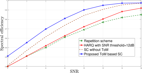
Figure 3: Spectral efficiency vs SNR for different SC schemes.

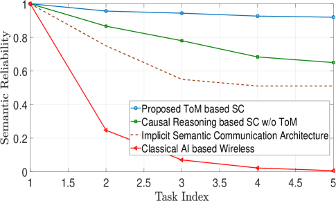
Figure 4: Semantic reliability vs SNR varying tasks.

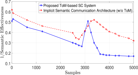
Figure 5: Semantic effectiveness vs number of samples, with task changing around $3K$ samples.

V Conclusion

In this paper, we have presented a new vision of semantic communication systems that relies upon ToM as a machinery to enable dynamic updates of the NN components at the transmit and receive side. We have formulated a ToM based joint transmit and receive design to learn an optimal representation space for transmission and extracting the semantic state description at the listener. The optimized AI components at the transmit side herein can be dynamically fine-tuned using the semantic level feedback from the receive side. The causal discovery component at the transmitter is implemented using the GNN and is learned as a directed acyclic graph. Simulation results have demonstrated superiority of our proposed SC in terms of improving the communication efficiency (minimal transmission) and reliability compared to classical communication and state of the art semantic communication.

References

- [1] C. Chaccour, M. N. Soorki, W. Saad, M. Bennis, and P. Popovski, “Can Terahertz Provide High-Rate Reliable Low-Latency Communications for Wireless VR,” IEEE Internet of Things Journal, vol. 9, no. 12, pp. 9712–9729, Jun. 2022.
- [2] C. Chaccour, W. Saad, M. Debbah, Z. Han, and H. V. Poor, “Less Data, More Knowledge: Building Next Generation Semantic Communication Networks,” arXiv preprint arXiv:2211.14343, Nov. 2022.
- [3] E. C. Strinati and S. Barbarossa, “6G Networks: Beyond Shannon Towards Semantic and Goal-Oriented Communications,” Computer Networks, Elsevier, vol. 190, May 2021.
- [4] E. Uysal, O. Kaya, A.Ephremides, J. Gross, M. Codreanu, P. Popovski, M. Assad, G. Liva, A. Munari, B. Soret, and T. Soleymani, “Semantic Communications in Networked Systems: A Data Significance Perspective,” IEEE Network, vol. 36, no. 4, pp. 233–240, Oct. 2022.
- [5] H. Xie, Z. Qin, G. Y. Li, and B-H. Juang, “Deep Learning Enabled Semantic Communication Systems,” IEEE Transactions on Signal Processing, vol. 69, pp. 2663–2675, Apr. 2021.
- [6] M. K. Farshbafan, W. Saad, and M. Debbah, “Curriculum Learning for Goal-Oriented Semantic Communications with a Common Language,” arXiv preprint arXiv:2111.08051, Feb. 2022.
- [7] M. Sana and E. C. Strinati, “Learning Semantics: An Opportunity for Effective 6G Communications,” in Proceedings of IEEE 19th Annual Consumer Communications and Networking Conference (CCNC), 2022, pp. 631–636.
- [8] E. Calvanese Strinati, “Semantic Data Exchange System with A Semantic Retransmission Channel ,” French Patent FR3111199, European Patent EP3923138, US patent US11706291, 24th, Aug. 2020.
- [9] P. Popovski, O. Simeone, F. Boccardi, D. Gündüz, and O. Sahin, “Semantic-Effectiveness Filtering and Control for Post-5G Wireless Connectivity ,” Journal of the Indian Institute of Science, vol. 100, no. 2, pp. 435–443, Apr. 2020.
- [10] C. K. Thomas and W. Saad, “Neuro-Symbolic Causal Reasoning Meets Signaling Game for Emergent Semantic Communications,” IEEE Transactions on Wireless Communications, Oct. 2023.
- [11] L. Yuan, Z. Fu, L. Zhou, K. Yang, and S-C Zhu, “Emergence of Theory of Mind Collaboration in Multiagent Systems,” arXiv preprint arXiv:2110.00121, pp. 424–438, 2021.
- [12] F. Scarselli, M. Gori, A. C. Tsoi, M. Hagenbuchner, and G. Monfardini, “The Graph Neural Network Model,” IEEE Transactions on Neural Networks, vol. 20, no. 1, pp. 561–80, Dec. 2008.
- [13] G. Dudek and N. Roy, “Multi-Robot Rendezvous in Unknown Environments,” in Proceedings of the AAAI National Conference Workshop on Online Search, Providence, Rhode Island, USA, 2009, pp. 22–29.
- [14] E. Bareinboim, J. D. Correa, D. Ibeling, and T. Icard, “On Pearl’s Hierarchy and the Foundations of Causal Inference,” in Probabilistic and Causal Inference: The Works of Judea Pearl (ACM Books), 2020.
- [15] D. Hafner, T. Lillicrap, T. Fischer, T. Villegas D. Ha, H. Lee, and J. Davidson, “Learning Latent Dynamics for Planning from Pixels,” Proceedings of the 36th International Conference on Machine Learning (PMLR), vol. 97, Jun. 2019.
- [16] C. K. Thomas, W. Saad, and Y. Xiao, “Causal Semantic Communication for Digital Twins: A Generalizable Imitation Learning Approach,” arXiv e-prints. Apr:arXiv-2304, 2023.
- [17] C. W. J. Granger, “Investigating Causal relations by Econometric Models and Cross-spectral Methods,” Journal of the Econometric Society, pp. 424–438, 1969.
- [18] C. W. Fox and S. J. Roberts, “A Tutorial on Variational Bayesian Inference,” Artificial intelligence review, vol. 38, pp. 85–95, 2012.
- [19] M. Warglien and P. Gärdenfors, “Semantics, Conceptual Spaces, and the Meeting of Minds.,” Synthese, vol. 190, no. 12, pp. 2165–2193, 2013.
- [20] L. Yuan, Z. Fu, L. Zhou, K. Yang, and S-C Zhu, “Emergence of Theory of Mind Collaboration in Multiagent Systems,” in 33rd Conference on Neural Information Processing Systems (NeurIPS), Vancouver, Canada, Dec. 2019.
- [21] T. Y. Tung, D. B. Kurka, M. Jankowski, and D. Gündüz, “DeepJSCC-Q: Constellation Constrained Deep Joint Source-Channel Coding,” IEEE Journal on Selected Areas in Information Theory, vol. 3, pp. 720 – 731, 2022.
- [22] J. Chung, C. Gulcehre, K. Cho, and Y. Bengio, “Empirical Evaluation of Gated Recurrent Neural Networks on Sequence Modeling,” arXiv preprint arXiv:1412.3555, 2014.
- [23] Y. Xiao, Z. Sun, G. Shi, and D. Niyato, “Imitation Learning-based Implicit Semantic-aware Communication Networks: Multi-layer Representation and Collaborative Reasoning,” IEEE Journal on Selected Areas in Communications, vol. 43, no. 1, Mar. 2023.
- [24] E. Bourtsoulatze, D. B. Kurka, and D. Gündüz, “Deep Joint Source-Channel Coding for Wireless Image Transmission,” IEEE Transactions on Cognitive Communications and Networking, vol. 5, no. 3, pp. 567–579, 2019.