Analytic approach to astrometric perturbations of critical curves by substructures

Abstract

Astrometric perturbations of critical curves in strong lens systems are thought to be one of the most promising probes of substructures down to small-mass scales. While a smooth mass distribution creates a symmetric geometry of critical curves with radii of curvature about the Einstein radius, substructures introduce small-scale distortions on critical curves, which can break the symmetry of gravitational lensing events near critical curves, such as highly magnified individual stars. We derive a general formula that connects the fluctuation of critical curves with the fluctuation of the surface density caused by substructures, which is useful when constraining models of substructures from observed astrometric perturbations of critical curves. We numerically check that the formula is valid and accurate as long as substructures are not dominated by a small number of massive structures. As a demonstration of the formula, we also explore the possibility that an anomalous position of an extremely magnified star, recently reported as ‘Mothra’, can be explained by fluctuations in the critical curve due to substructures. We find that cold dark matter subhalos with masses ranging from $5\times 10^{7}M_{\odot}/h$ to $10^{9}M_{\odot}/h$ can well explain the anomalous position of Mothra, while in the fuzzy dark matter model, the very small mass of $\sim 10^{-24}$ eV is needed to explain it.

I Introduction

Substructures within dark matter (DM) halos have been intensively studied in recent decades, motivated by a wide range of topics in cosmology. The abundance and distribution of substructures provide valuable insight into primordial perturbations, which are the initial seeds of cosmological structures. While observations of the cosmic microwave background and the large-scale structures have tightly constrained statistical properties of primordial perturbations on scales approximately larger than $1$ Mpc, or roughly higher than $10^{13}M_{\odot}$ in terms of mass of DM halos, our understanding of smaller scales, specifically those corresponding to substructures, remains limited [1, 2, 3, 4].

Properties of substructures can also potentially reflect the properties of DM. While current observations, especially of large-scale structures, strongly support cold dark matter (CDM), several deviations from the CDM prediction have been reported at smaller scales (see Refs. [5, 6] for review), which may hint alternatives to CDM, such as warm dark matter [7, 8, 9] and dark matter with a macroscopic de Broglie wavelength, referred to as fuzzy dark matter (FDM) [10, 11, 12, 13]. In the CDM paradigm, masses of substructures span a wide range, from approximately $10^{-6}M_{\odot}$ to around $10^{16}M_{\odot}$. In contrast, warm dark matter or FDM predict characteristic mass scales that preclude the formation of smaller substructures. FDM also predicts specific shapes of substructures, such as clumps resulting from quantum interference patterns and cores resulting from quantum pressure, often referred to as soliton cores. Therefore, detailed studies of substructures down to small mass scales may provide an important clue to the nature of DM.

One promising method to study substructures down to small mass scales is to use gravitational lensing effects [14]. In particular, strong gravitational lensing effects, which exhibit high magnification and multiple images of the distant source, are affected by substructures inside primary lens objects, such as massive galaxies and galaxy clusters. Several studies pointed out a link between strong gravitational lensing systems with anomalous flux ratios and substructures inside lens objects [15, 16, 17, 18, 19, 20, 21, 22, 23, 24]. In Ref. [24], they analyzed seven gravitational lensing events of radio quasars which show flux anomalies using the lens model, including substructures, stellar discs and line-of-sight haloes. Then they found a mass fraction of substructures $f_{\mathrm{sat}}$ as $0.8\%<f_{\mathrm{sat}}<1.9\%$, at the $68\%$ confidence level, with a median estimation of $f_{\mathrm{sat}}=1.2\%$, which is in agreement with the predictions from CDM hydrodynamical simulations within $1\sigma$. In addition, substructures can also be probed by observing the distortions in the surface brightness patterns of lensed giant arcs [25, 26, 27, 28].

Dai et al. [29] proposed a new method to search for substructures inside galaxy clusters focusing on astrometric perturbations. A smooth mass distribution creates a geometry that yields multiple images with symmetric configurations and critical curves with radii of curvature about the Einstein radius. Hereafter, we refer to such lens models as ‘macro’-lens models. The existence of substructures introduces small-scale distortions on such a macro-critical curve, which can distort or break the symmetry of the gravitational lensing events expected from the macro-critical curve. Such distortions of macro-critical curves can be probed by highly magnified individual stars that are observed in the vicinity of critical curves [30, 31]. It is argued that CDM subhalos of masses ranging from $10^{6}M_{\odot}$ to $10^{8}M_{\odot}$ produce fluctuations of the macro-critical curve that could be detected with $\sim 10$ hr integrations with the James Webb Space Telescope (JWST) in near-infrared bands (see also Ref. [32]).

In this paper, we derive a general formula that connects fluctuations in macro-critical curves with the fluctuation of the surface density caused by substructures. This formula allows us to analytically estimate the amplitude of the fluctuations from the surface density power spectrum of substructures, which is useful for discussing the mass of the substructures in the context of astrometric perturbations. As for the surface density power spectrum, previous studies have proposed the expressions for the different types of substructures such as CDM subhalos  [26] and quantum clumps of FDM [33]. We verify the validity of this formula by performing numerical simulations.

Recently, Diego et al. [34] reported an anomaly of an extremely magnified (likely binary) star, nicknamed ’Mothra’, in which the counterimage is not seen yet even though nearby stars are found in set with their counterimages (see Fig. 2 in Ref. [34]). They have argued that the anomaly could be explained by considering a local millilensing effect caused by a substructure. In this paper, as an immediate application of our formula, we discuss the possibility of explaining the Mothra’s anomalous observed position by fluctuations in the macro-critical curve due to substructures such as CDM subhalos and quantum clumps of FDM.

This paper is organized as follows. In Sect. II, we first review the macro-lens model and derive the general formula connecting fluctuations in macro-critical curves with the fluctuation of the surface density caused by substructures from the lens equation. In Sect. III, we numerically verify the formula and examine a parameter region in which this formula is accurate. In Sect. IV, we attempt an alternative interpretation of the anomalous lensing events utilizing the formula. In Sect. V, we conclude this paper.

Throughout this paper, we assume a flat $\Lambda$CDM cosmology and fix cosmological parameters to the Planck 2018 best-fit values [4].

II Fluctuations of macro-critical curves

To study fluctuations of macro-critical curves by substructures, let us first define a macro-lens model in which we set the origin of the coordinate system in the image and source planes on the critical curve and the caustic, respectively.

The lens equation relates the source position $\bm{\beta}=(\beta_{x},\beta_{y})$ with the image position $\bm{\theta}=(\theta_{x},\theta_{y})$ as

$$\begin{split}\bm{\beta}=\bm{\theta}-\nabla\psi(\bm{\theta}),\end{split}$$ (1)

with $\psi(\bm{\theta})$ being the lens potential. By expanding the lens potential up to the third order at the origin, we obtain

$$\begin{split}\begin{aligned} \psi(\bm{\theta})&=\frac{1}{2}\left(\psi_{,xx}\theta_{x}^{2}+2\psi_{,xy}\theta_{x}\theta_{y}+\psi_{,yy}\theta_{y}^{2}\right)\\ &+\frac{1}{6}\left(\psi_{,xxx}\theta_{x}^{3}+3\psi_{,xxy}\theta_{x}^{2}\theta_{y}+3\psi_{,xyy}\theta_{x}\theta_{y}^{2}+\psi_{,yyy}\theta_{y}^{3}\right),\end{aligned}\end{split}$$ (2)

where the subscription of $,x$ and $,y$ represents the derivative with respect to $\theta_{x}$ and $\theta_{y}$, respectively. Here, we drop the leading two terms by setting the origin of the image plane to the origin of the source plane. We denote the convergence at the origin as $\kappa_{0}$, which satisfies

$$\begin{split}\kappa_{0}=\frac{1}{2}(\psi_{,xx}+\psi_{,yy}).\end{split}$$ (3)

With the condition that the critical curve and the caustic pass through the origin and using Eq. (3), one can obtain

$$\begin{split}&\psi_{,xx}=\kappa_{0}+\left(1-\kappa_{0}\right)\cos\omega,\\ &\psi_{,yy}=\kappa_{0}-\left(1-\kappa_{0}\right)\cos\omega,\\ &\psi_{,xy}=-\left(1-\kappa_{0}\right)\sin\omega,\end{split}$$ (4)

using the arbitrary constant parameter $\omega$. For simplicity, we set $\omega=0$ in this work. Additionally, we henceforward consider a complete orthogonal coordinate system in which the critical curve and multiple images are perpendicular to each other by setting $\psi_{,xxy}=\psi_{,xyy}=\psi_{,yyy}=0$. Denoting $\psi_{,xxx}=\epsilon$, the lens potential can be written by

$$\begin{split}\psi(\bm{\theta})=\frac{1}{2}\left[\kappa_{0}\left(\theta_{x}^{2}+\theta_{y}^{2}\right)+\left(1-\kappa_{0}\right)\left(\theta_{x}^{2}-\theta_{y}^{2}\right)\right]-\frac{\epsilon}{6}\theta_{x}^{3}.\end{split}$$ (5)

With this lens potential, the lens equation becomes very simple as

$$\begin{split}\begin{aligned} &\beta_{x}=\frac{\theta_{x}^{2}}{2}\epsilon,\\ &\beta_{y}=2\left(1-\kappa_{0}\right)\theta_{y}.\end{aligned}\end{split}$$ (6)

Note that $\epsilon$ has the dimension of the inverse of the angle, whose value approximately corresponds to the inverse of the Einstein radius of the macro-lens model. The Jacobian matrix is written by

$$\begin{split}\left(\frac{\partial\bm{\beta}(\bm{\theta})}{\partial\bm{\theta}}\right)=\begin{pmatrix}\epsilon\theta_{x}&0\\ 0&2(1-\kappa_{0})\\ \end{pmatrix}.\end{split}$$ (7)

One can find that the $\theta_{y}$-axis corresponds to the critical curve by calculating the determinant of the matrix in Eq. (7).

Now, let us consider the fluctuations of the macro-critical curve due to substructures. Considering fluctuations of a point on the original critical curve (i.e., $\tilde{\bm{\theta}}=(\delta\theta_{x},\theta_{y}+\delta\theta_{y})$) caused by substructures, the Jacobian matrix up to linear order is given by

$$\begin{split}\left(\frac{\partial\bm{\beta}(\tilde{\bm{\theta}})}{\partial\bm{\theta}}\right)\approx\begin{pmatrix}\epsilon\delta\theta_{x}-\delta\kappa-\delta\gamma_{1}&-\delta\gamma_{2}\\ -\delta\gamma_{2}&2(1-\kappa_{0})-\delta\kappa+\delta\gamma_{1}\\ \end{pmatrix},\end{split}$$ (8)

where $\delta\kappa$, $\delta\gamma_{1}$, and $\delta\gamma_{2}$ represent the convergence and two components of the shear due to substructures, respectively. The determinant of the Jacobian matrix is given by

$$\begin{split}\mathrm{det}&\left(\frac{\partial\bm{\beta}(\tilde{\bm{\theta}})}{\partial\bm{\theta}}\right)\\ &\ \approx(\epsilon\delta\theta_{x}-\delta\kappa-\delta\gamma_{1})\left(2(1-\kappa_{0})-\delta\kappa+\delta\gamma_{1}\right)-\delta\gamma_{2}^{2}\\ &\ \approx 2(1-\kappa_{0})(\epsilon\delta\theta_{x}-\delta\kappa-\delta\gamma_{1}).\end{split}$$ (9)

Since the determinant must be equal to zero, the fluctuated critical curve satisfies

$$\begin{split}\delta\theta_{x}=\frac{1}{\epsilon}(\delta\kappa+\delta\gamma_{1}).\end{split}$$ (10)

From Eq. (10), we obtain the power spectrum of $\delta\theta_{x}$ as

$$\begin{split}P_{\delta\theta_{x}}=\frac{1}{\epsilon^{2}}\left(P_{\delta\kappa}+2P_{\delta\kappa\delta\gamma_{1}}+P_{\delta\gamma_{1}}\right),\end{split}$$ (11)

where $P_{\delta\theta_{x}}$, $P_{\delta\kappa}$, and $P_{\delta\gamma_{1}}$ are the auto two-dimensional power spectrum of $\delta\theta_{x}$, $\delta\kappa$, and $\delta\gamma_{1}$, respectively, and $P_{\delta\kappa\delta\gamma_{1}}$ represents the cross power spectrum between $\delta\kappa$ and $\delta\gamma_{1}$. Here, we define the two-dimensional power spectrum of $X$ and $Y$ as

$$\begin{split}\braket{X(\bm{k})Y(\bm{k}^{\prime})}=(2\pi)^{2}\delta^{\mathrm{2D}}(\bm{k}+\bm{k}^{\prime})P_{XY},\end{split}$$ (12)

where $\bm{k}$ is a wavenumber on a two-dimensional plane.

Using the relations between $\delta\kappa$ and $\delta\gamma_{1}$,

$$\begin{split}P_{\delta\gamma_{1}}=\cos^{2}(2\phi_{\ell})P_{\delta\kappa},\\ P_{\delta\kappa\delta\gamma_{1}}=\cos(2\phi_{\ell})P_{\delta\kappa},\end{split}$$ (13)

we obtain

$$\begin{split}P_{\delta\theta_{x}}=\frac{1}{\epsilon^{2}}(1+2\cos(2\phi_{\ell})+\cos^{2}(2\phi_{\ell}))P_{\delta\kappa},\end{split}$$ (14)

where $\phi_{\ell}$ is the azimuthal polar. Taking average of $\phi_{\ell}$, we finally obtain

$$\begin{split}P_{\delta\theta_{x}}=\frac{3}{2\epsilon^{2}}P_{\delta\kappa},\end{split}$$ (15)

and

$$\begin{split}\epsilon^{2}\braket{\delta\theta_{x}^{2}}=\frac{3}{2}\int d\log k~{}\frac{k^{2}}{2\pi}P_{\delta\kappa}=\frac{3}{2}\braket{\delta\kappa^{2}}.\end{split}$$ (16)

Note that $\epsilon^{2}\braket{\delta\theta_{x}^{2}}\approx\braket{\delta\theta_{x}^{2}}/\theta_{\mathrm{Ein}}^{2}$, given that $\epsilon\approx 1/\theta_{\mathrm{Ein}}$. Deriving these simple formulae of Eqs (15) and (16) is the main result in this paper. Although previous work has derived a formula between fluctuations of image positions and the surface density perturbations from substructures [19], as far as we are aware, this is the first time to derive the formulae between the critical curve fluctuations and the surface density perturbations. These formulae allow us to analytically estimate the variance of $P_{\delta\theta_{x}}$ or $\braket{\delta\theta_{x}^{2}}^{1/2}$ from the surface density power spectrum of substructures, $P_{\delta\kappa}$.

While Eq. (15) is derived assuming a complete orthogonal coordinate system, we argue that Eq. (15) holds rather generically because near the fold critical curve tangential and radial magnifications generally behaves as [35]

$$\begin{split}\mu_{\mathrm{t}}\approx\frac{\mu_{\mathrm{t0}}}{\delta\theta},\quad\mu_{\mathrm{r}}\approx\mathrm{const}.,\end{split}$$ (17)

where $\delta\theta$ denotes the distance from the critical curve. Since the tangential magnification is defined by $\mu_{\mathrm{t}}^{-1}=1-\kappa-\gamma$ with $\gamma=\sqrt{\gamma_{1}^{2}+\gamma_{2}^{2}}$, substructures modify the inverse of the tangential magnification as

$$\begin{split}\mu_{\mathrm{t}}^{-1}\approx\frac{\delta\theta}{\mu_{\mathrm{t0}}}-\delta\kappa-\frac{\gamma_{1}}{\gamma}\delta\gamma_{1}-\frac{\gamma_{2}}{\gamma}\delta\gamma_{2}.\end{split}$$ (18)

Since the perturbed critical curve satisfies $\mu_{\mathrm{t}}^{-1}=0$, we obtain

$$\begin{split}P_{\delta\theta}&=\mu_{\mathrm{t0}}^{2}\left[P_{\delta\kappa}+\left(\frac{\gamma_{1}}{\gamma}\right)^{2}P_{\delta\gamma_{1}}+\left(\frac{\gamma_{2}}{\gamma}\right)^{2}P_{\delta\gamma_{2}}\right]\\ &=\frac{3\mu_{\mathrm{t0}}^{2}}{2}P_{\delta\kappa},\end{split}$$ (19)

where we take an average of $\phi_{\ell}$. Equation (19) is essentially same as Eq. (15) if $\mu_{\mathrm{t0}}=1/\epsilon$.

While our analytic results are applicable to any form of substructures, here let us describe a specific form of $P_{\delta\kappa}(k)$ when substructures are CDM subhalos. Using the halo formalism [36] and assuming that the spatial correlation between subhalos can be negligible (i.e., subhalos are randomly distributed), we can compute the surface density power spectrum as an integral over the mass function weighted by their surface density profile as [26]

$$\begin{split}P_{\delta\kappa}(k)=\int^{M_{\mathrm{max}}}_{M_{\mathrm{min}}}\frac{dn^{\mathrm{2D}}}{dM}\left|\tilde{\kappa}_{M}(k)\right|^{2}dM,\end{split}$$ (20)

where $k=\sqrt{k_{x}^{2}+k_{y}^{2}}$, $M_{\mathrm{min}}$ and $M_{\mathrm{max}}$ are the minimum and maximum mass of subhalos, respectively, $dn^{\mathrm{2D}}/dM$ is the surface number density of subhalos with masses of $[M,M+\delta M]$, and $\tilde{\kappa}_{M}(k)$ is the Fourier transform of the convergence $\kappa_{M}$ provided by a subhalo of mass $M$. Here $\tilde{\kappa}_{M}(k)$ can be calculated by

$$\begin{split}\tilde{\kappa}_{M}(k)=\frac{M\tilde{u}_{M}(\bm{K}_{*}=(k_{x},k_{y},0))}{\Sigma_{\rm cr}},\end{split}$$ (21)

where $\Sigma_{\rm cr}$ is the critical surface density, and $\tilde{u}_{M}(\bm{K})$ is the Fourier transform of their three-dimensional density profile, $\rho_{M}$, (see Appendix A),

$$\begin{split}\tilde{u}_{M}(\bm{K})&=\int_{0}^{R_{\mathrm{vir}}}\frac{4\pi R^{2}}{M}\frac{\sin KR}{KR}\rho_{M}(R)\mathrm{d}R,\end{split}$$ (22)

where $K=|\bm{K}|$. In this paper, we simply adopt the ordinal Navarro-Frenk-White (NFW) profile [37], which is defined by

$$\begin{split}\rho_{\mathrm{NFW}}(R)=\frac{Mc_{\mathrm{vir}}^{3}}{4\pi R_{\mathrm{vir}}^{3}}\frac{f_{\mathrm{NFW}}(c_{\mathrm{vir}})}{\left(Rc_{\mathrm{vir}}/R_{\mathrm{vir}}\right)\left(1+Rc_{\mathrm{vir}}/R_{\mathrm{vir}}\right)^{2}},\end{split}$$ (23)

where $R_{\mathrm{vir}}$ is the virial radius, $c_{\mathrm{vir}}$ is the concentration parameter for virial radius, and $f_{\mathrm{NFW}}(c)\equiv 1/[\ln(1+c)-c/(1+c)]$. Then $\tilde{u}_{M}(K)$ can be expressed by [38],

$$\begin{split}\tilde{u}_{M}(K)&=f_{\mathrm{NFW}}(c_{\mathrm{vir}})\Biggl{\{}\sin\mathcal{K}[\operatorname{Si}(\mathcal{K}(1+c_{\mathrm{vir}}))-\operatorname{Si}(\mathcal{K})]\\ &~{}+\cos\mathcal{K}[\operatorname{Ci}(\mathcal{K}(1+c_{\mathrm{vir}}))-\operatorname{Ci}(\mathcal{K})]-\frac{\sin(\mathcal{K}c_{\mathrm{vir}})}{\mathcal{K}(1+c_{\mathrm{vir}})}\Biggr{\}},\end{split}$$ (24)

with $\mathcal{K}\equiv KR_{\mathrm{vir}}$, the sine integral functions, $\operatorname{Si}(X)=\int_{0}^{X}dt\sin(t)/t$, and the cosine integral function, $\operatorname{Ci}(X)=-\int_{X}^{\infty}dt\cos(t)/t$.

III Validity of the formula connecting $\braket{\delta\theta^{2}}$ and $\braket{\delta\kappa^{2}}$

In the previous section, we derive Eqs. (15) and (16), the simple analytical relations between fluctuations of the macro-critical curve and the fluctuation of the surface density due to substructures. Here, we check the validity of Eq. (16) by comparing it with direct numerical estimations of fluctuations of macro-critical curves due to substructures.

We first set up macro-lens models. We assume that the macro-lens object is a DM halo with a mass of $M_{\mathrm{hh}}=10^{15}~{}M_{\odot}/h$ located at redshift $z_{\mathrm{l}}=0.5$. We here focus on the tiny surface area near the critical curve caused by the DM halo adopting the lens potential defined by Eq. (5) with $\epsilon=1/$10\text{\,}\mathrm{\SIUnitSymbolArcsecond}$$ and the convergence $\kappa_{0}=0.5$.

We next set up lens models of substructures hosted by the DM halo. As an example, we here consider CDM subhalos as substructures. For the mass distribution of subhalos, we adopt the NFW profile in Eq. (23) with the concentration parameter computed by the mass-concentration relation presented in Ref. [39]. Note that we multiply the concentration parameter by $\left[200/\Delta_{\mathrm{vir}}\Omega_{\mathrm{m}}(z)\right]^{1/3}\left[H(z)/H_{0}\right]^{-2/3}$ with the virial overdensity computed from the spherical collapse model, $\Delta_{\mathrm{vir}}$, to convert from $c_{200}$ to $c_{\mathrm{vir}}$ [40].

We also assume that the density profile of the DM halo follows the NFW density profile, and the spatial distribution of subhalos also follows it. The surface number density of subhalos is then proportional to the surface NFW density as

$$\begin{split}n^{\mathrm{2D}}\equiv\frac{dN_{\mathrm{sub}}}{dS}\propto\Sigma_{\mathrm{NFW}}(r;M_{\mathrm{hh}}),\end{split}$$ (25)

where $dS=2\pi rdr$ with $r=\sqrt{x^{2}+y^{2}}$, $\Sigma_{\mathrm{NFW}}(r)$ is the surface density of the NFW profile. The concentration parameter for the host halos is estimated by the mass-concentration relation presented in Ref. [41]. The surface number density of subhalos with masses of $[M,M+\delta M]$ in Eq. (20) is given by

$$\begin{split}\frac{dn^{\mathrm{2D}}}{dM}=\frac{dN_{\mathrm{sub}}}{dM}\frac{\Sigma_{\mathrm{NFW}}(r;M_{\mathrm{hh}})}{M_{\mathrm{hh}}},\end{split}$$ (26)

where $dN_{\mathrm{sub}}/dM$ shows the total number of subhalos with masses of $[M,M+\delta M]$ inside their host halo. We adopt a simple analytic model presented in Ref. [42] for calculating $dN_{\mathrm{sub}}/dM$. We assume that the spatial correlation among subhalos can be neglected and distribute them with a constant surface number density assuming the Poisson distribution, which is justified by the tiny surface area in the vicinity of the critical curve considered here. This assumption may be validated by the fact that subhalos are exposed to the tidal gravity of their host halo.

Distributing CDM subhalos near the macro-critical curve by the Poisson distribution with the expected number from Eq. (26), we numerically calculate fluctuations of the macro-critical curves. We use an open software, Glafic code, presented in Refs. [43, 44]. To distribute subhalos, it is necessary to set $M_{\mathrm{min}}$ and $M_{\mathrm{max}}$ and the box size considered here. We explore six models with different sets of $(M_{\mathrm{min}},M_{\mathrm{max}})$ summarized in Table 1. The box size is basically set to $$3.0\text{\,}\mathrm{\SIUnitSymbolArcsecond}$\times$3.0\text{\,}\mathrm{\SIUnitSymbolArcsecond}$$ with the exception of $$1.5\text{\,}\mathrm{\SIUnitSymbolArcsecond}$\times$1.5\text{\,}\mathrm{\SIUnitSymbolArcsecond}$$ for model (b). These box sizes are determined for numerical reasons.

Table 1: Our models with different $(M_{\mathrm{min}},M_{\mathrm{max}})$ for the validation. We show numerical results as well as analytically estimated values of $\braket{\theta_{x}^{2}}^{1/2}$ by Eq. (16) for individual models.

Model	$M_{\mathrm{min}}~{}[M_{\odot}/h]$	$M_{\mathrm{max}}~{}[M_{\odot}/h]$	Numerical results	Analytic value	Remark
(a)	$5\times 10^{6}$	$10^{8}$	$0.0459\pm 0.0123$	$0.0422$	$$3.0\text{\,}\mathrm{\SIUnitSymbolArcsecond}$\times$3.0\text{\,}\mathrm{\SIUnitSymbolArcsecond}$$, 10 realizations
(b)	$10^{6}$	$10^{8}$	$0.0476\pm 0.0114$	$0.0467$	$$1.5\text{\,}\mathrm{\SIUnitSymbolArcsecond}$\times$1.5\text{\,}\mathrm{\SIUnitSymbolArcsecond}$$, 10 realizations
(c)	$5\times 10^{6}$	$10^{9}$	$0.0629\pm 0.0141$	$0.0730$	$$3.0\text{\,}\mathrm{\SIUnitSymbolArcsecond}$\times$3.0\text{\,}\mathrm{\SIUnitSymbolArcsecond}$$, 10 realizations
(d)	$5\times 10^{6}$	$10^{10}$	$0.0995\pm 0.0320$	$0.119$	$$3.0\text{\,}\mathrm{\SIUnitSymbolArcsecond}$\times$3.0\text{\,}\mathrm{\SIUnitSymbolArcsecond}$$, 10 realizations
(e)	$5\times 10^{6}$	$10^{11}$	$0.112\pm 0.044$	$0.186$	$$3.0\text{\,}\mathrm{\SIUnitSymbolArcsecond}$\times$3.0\text{\,}\mathrm{\SIUnitSymbolArcsecond}$$, 10 realizations
(f)	$5\times 10^{6}$	$10^{12}$	$0.129\pm 0.041$	$0.291$	$$3.0\text{\,}\mathrm{\SIUnitSymbolArcsecond}$\times$3.0\text{\,}\mathrm{\SIUnitSymbolArcsecond}$$, 10 realizations

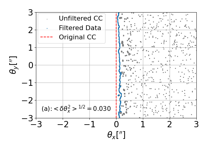
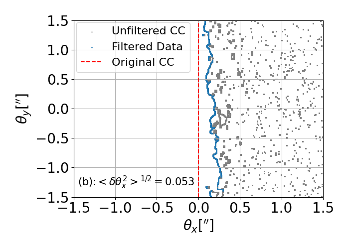
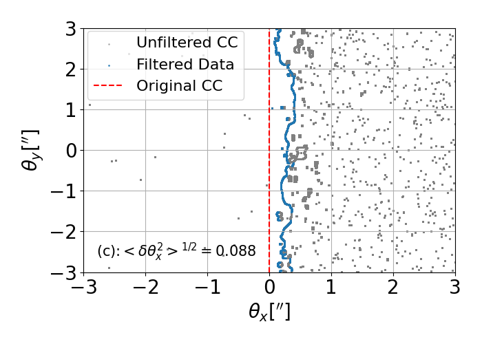
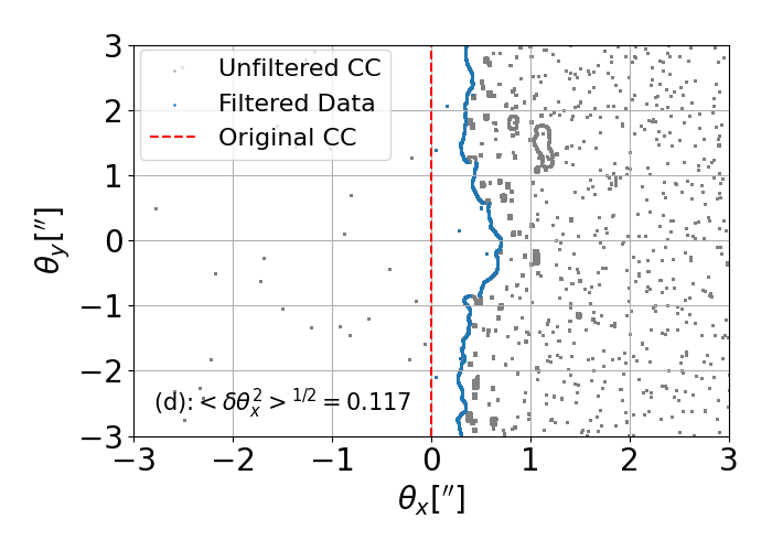
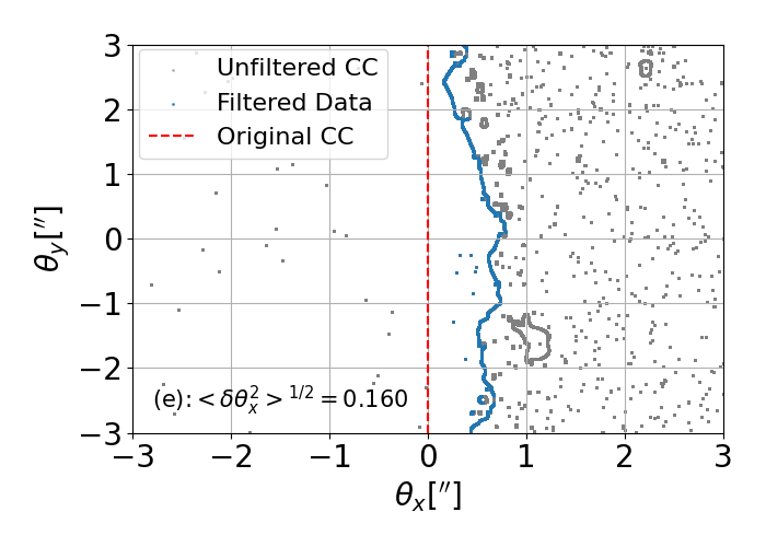
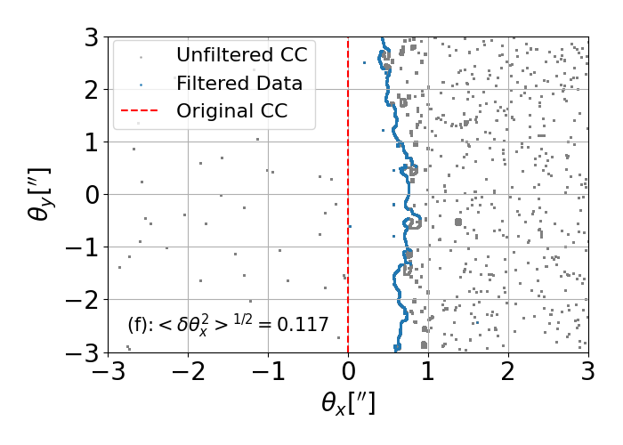
Figure 1: An example of fluctuated critical curves by CDM subhalos for each model summarized in Tab. 1. The red dashed vertical line shows the original macro-critical curve described in Sect. II. The grey points show critical curves calculated in Glafic, while the blue points show the fluctuated critical curves obtained by filtering, as explained in the text. The value of $\braket{\delta\theta_{x}^{2}}^{1/2}$ shows the standard deviation of $\theta_{x}$ for each panel. For the mean value of each model, see Tab. 1. Top left: Model (a), Top right: Model (b), Middle left: Model (c), Bottom right: Model (d), Bottom left: Model (e), Bottom right: Model (f).

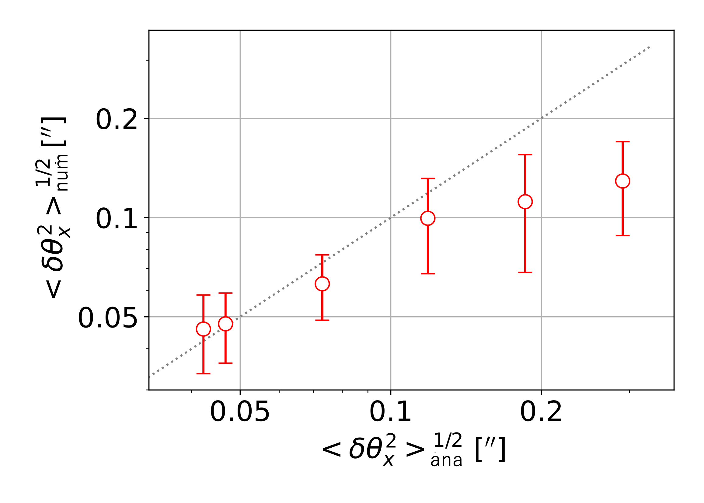
Figure 2: Comparison between analytically calculated values of $\braket{\delta\theta_{x}^{2}}^{1/2}$ from Eq. (16) and the ones numerically estimated using Glafic. Here we set $M_{\mathrm{hh}}=10^{15}~{}M_{\odot}/h$.

For each model of $(M_{\mathrm{min}},M_{\mathrm{max}})$, we run the calculations for ten realizations. From the obtained critical curves, we take the mean and variance of the fluctuations $\braket{\theta_{x}^{2}}^{1/2}$. A caveat is that Glafic outputs isolated critical curves that are associated with subhalos as well. In order to compute fluctuations of macro-model critical curves that are our main interest here, those critical curves associated with subhalos must be removed. To do so, we adopt a simple filtering method with three steps: (1) sorting points representing critical curves by $\theta_{y}$ coordinate, (2) subdividing the sorted points into several blocks with $\mathcal{O}(10^{2})$ data points, and (3) acquiring only the point with the smallest $\theta_{x}$ in each block. Figure 1 shows the resulting fluctuated critical curves for each model. In Fig. 1, the red dashed line shows the original macro-critical curve described in Sect. II. The grey points depict critical curves calculated in Glafic. The blue points show the fluctuated critical curves obtained by the filtering method described above. We find that the original critical curves are shifted in the positive direction of the $\theta_{x}$-axis. This is explained by the contribution of the additional mass of subhalos that moves the macro critical curve to the outer radii, which corresponds to the position $\theta_{x}$ in this coordinate system.

Table 1 also shows the numerical results of $\braket{\theta_{x}^{2}}^{1/2}$ estimated in the manner described above. We find that the values of $\braket{\theta_{x}^{2}}^{1/2}$ for models of (a)-(d) agree well with the analytically estimated values from Eq. (16). When the $M_{\mathrm{max}}$ becomes larger than $10^{10}M_{\odot}$, the numerically estimated values become smaller than the analytically estimated ones. This deviation may come from the non-Gaussianity due to massive subhalos; the probability of their existence is rare, i.e., there seldom exists such massive subhalos in our calculation box, while their analytical contribution to $\braket{\kappa^{2}}$ is significant. Alternatively, our filtering method to pick the smallest-$\theta_{x}$ data point in each block could lead to systematic underestimations in some simulations. In either case, we conclude that Eq. (16) is valid and accurate, at least as long as the substructure power spectrum is not dominated by a small number of massive structures. We summarize the comparison between the numerical and analytic values from Eq. (16) in Fig. 2.

IV Application to Mothra

This section will apply the formula in Eq. (16) for discussing the origin of an extremely magnified binary star at redshift $z=2.091$ recently reported in Ref. [34] with JWST/NIRCam data, nicknamed ‘Mothra’. Mothra is found in the strong lensing region in the galaxy cluster of MACS J0416.1-403 at $z=0.397$. The Mothra, formally called LS1, is observed only on one side of the critical curve with negative parity, and its counterimage is not seen even though nearby star clusters are found in a pair on both sides of the critical curve as shown in Fig. 2 of Ref. [34].

Although Ref. [34] argued that the anomaly could be explained by considering a local millilensing effect due to a substructure that demagnifies and hides one of the multiple images of Mothra, we here attempt to interpret this anomaly as caused by fluctuations in the macro-critical curve due to substructures. In our new interpretation, Mothra is regarded as an event similar to Earendel [31] that is located exactly on the macro-critical curve and whose multiple images are unresolved, but due to a fluctuated macro-critical curve Mothra is observed in an apparently offset position. With our analytic formula, we check which substructure models can explain the observed offset of Mothra.

The macro-lens model for the Mothra is set up as follows. We adopt $z_{\mathrm{s}}=2.091$ and $z_{\mathrm{l}}=0.397$. According to Ref. [45], the virial halo mass of MACS J0416.1-403 is estimated as $(1.24\pm 0.28)\times 10^{15}M_{\odot}$. Using the Glafic mass model of MACS J0416.1-403 [43, 46], the Einstein radius for this source redshift is estimated as $\theta_{\mathrm{Ein}}\approx$24.13\text{\,}\mathrm{\SIUnitSymbolArcsecond}$$. Combining the Einstein radius and the mass of the galaxy cluster, we also fix the concentration parameter $c_{\mathrm{vir}}=7.59$. Here, we assume the stellar-mass-halos-mass relation [47], galaxy-size relation [42], the Hernquist density profile for the stellar components [48], and the mass-concentration relation [41]. Note that the total stellar mass is estimated as $1.09\times 10^{12}M_{\odot}$, and the effective radius in the Hernquist profile is $\theta_{\mathrm{b}}=$1.22\text{\,}\mathrm{\SIUnitSymbolArcsecond}$$. The parameter $\epsilon$ should be determined by the local structure of the macro-model critical curve around Mothra. Again, we adopt the Glafic mass model to estimate the tangential magnification as a function of the distance from the macro-critical curve $\delta\theta$, finding $\mu_{\mathrm{t}}\approx$8\text{\,}\mathrm{\SIUnitSymbolArcsecond}$/\delta\theta$. Based on the discussion given in Sect. II, we set $\epsilon=1/$8\text{\,}\mathrm{\SIUnitSymbolArcsecond}$$ for our analytic estimates of fluctuations of macro-critical curves.

In our new interpretation, the macro-critical curve needs to be fluctuated by $\sim$0.07\text{\,}\mathrm{\SIUnitSymbolArcsecond}$$, especially to the negative parity side, as shown in Fig. 2 in Ref. [34]. Eq. (16) allows us to analytically estimate the fluctuation of the surface density power spectrum by substructures necessary to predict the fluctuation of the macro-critical curve needed to explain Mothra. We obtain $\braket{\delta\kappa^{2}}\sim 3.27\times 10^{-5}$ for $\braket{\delta\theta_{x}^{2}}^{1/2}\sim$0.07\text{\,}\mathrm{\SIUnitSymbolArcsecond}$$. In the following, we consider two cases as substructures as examples: CDM subhalos and quantum clumps of FDM halos.

IV.1 CDM subhalos

Combining Eq. (20) with Eq. (16), we estimate the parameter set of ($M_{\mathrm{min}}$, $M_{\mathrm{max}}$) needed to explain $\braket{\delta\kappa^{2}}\sim 3.27\times 10^{-5}$. We plot the contour of $\braket{\delta\theta_{x}^{2}}^{1/2}$ as a function of $M_{\mathrm{max}}$ and $M_{\mathrm{min}}/M_{\mathrm{max}}$ in Fig. 3. We find that models with $M_{\mathrm{max}}\sim 10^{8}-10^{9}~{}M_{\odot}/h$ well explain the observed offset of Mothra.

From Fig. 3, we choose a model with $(M_{\mathrm{min}},M_{\mathrm{max}})=(5\times 10^{7}~{}M_{\odot}/h,10^{9}~{}M_{\odot}/h)$, plotted in red cross, where the amplitude of the one-sigma fluctuation corresponds approximately to the offset of Mothra. This model has a sufficiently small $M_{\mathrm{max}}$ and satisfies the condition of no visible galaxy around Mothra. We examine this model further to investigate whether such fluctuations could affect the magnification ratio between $c$ and $c^{\prime}$, a nearby multiple image pair of a star cluster. As mentioned in Ref. [34], the magnification ratio should approximately correspond to the ratio of separations from $b$ to $c$ and from $b^{\prime}$ to $c^{\prime}$, $\sim(b-c)/(b^{\prime}-c^{\prime})\sim 0.39/0.32=1.22$. We numerically calculate fluctuated critical curves for this model in the same manner as in Sect. III by subdividing the data points and collecting only the point with the smallest $\theta_{x}$ in each block and, at the same time, record the values of the magnification $\mu$ at positions of $c$ and $c^{\prime}$ in each block. Running the calculations in ten realizations for each model, we take the 2000 parameter sets of $(\delta\theta_{x},\mu_{c},\mu_{c^{\prime}}).$

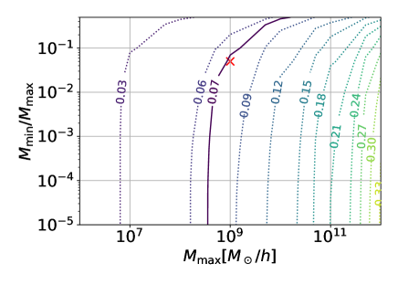
Figure 3: Contour of $\braket{\delta\theta_{x}^{2}}^{1/2}$ as a function of $M_{\mathrm{max}}$ and $M_{\mathrm{min}}/M_{\mathrm{max}}$ for the Mothra-like lens system. The value of each contour is shown in units of arcsec. The red cross shows the model that we calculate in detail to interpret the Mothra’s anomalous position.

Figure 4 shows the correlation between $\delta\theta_{x}$ and the magnification ratio $\mu_{c}/\mu_{c^{\prime}}$. The blue points show each parameter set, while the red dashed vertical line indicates the approximate required value of $\delta\theta_{x}$ to make the critical curve pass through the Mothra position. The red dashed horizontal line shows the magnification ratio between $c$ and $c^{\prime}$ expected from the distance ratio between $b-c$ and $b^{\prime}-c^{\prime}$. We find that there is no tight correlation between the value of $\delta\theta_{x}$ and $\mu_{c}/\mu_{c^{\prime}}$ and that there are models that satisfy both conditions.

Note that we must also consider perturbations of the image positions of $c,c^{\prime},b,$ and $b^{\prime}$ due to subhalos to confirm that those subhalos do not significantly affect observed positions of those additional multiple images. We leave it for future research.

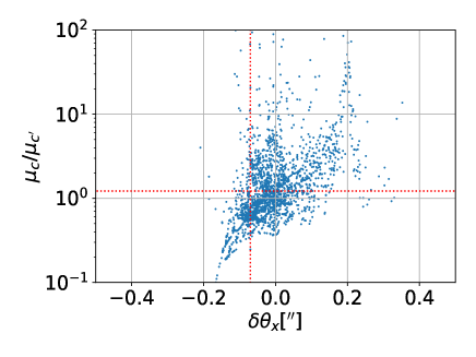
Figure 4: The correlation between $\delta\theta_{x}$ and the magnification ratio between $c$ and $c^{\prime}$, multiple image pair near Mothra. From the configuration of multiple images, the magnification ratio is predicted to be about $1.22$, represented by the horizontal red dotted line. The vertical red line shows the $\delta\theta_{x}$ to make the image at the Mothra’s offset an unresolved pair of images.

IV.2 Quantum clumps in FDM halos

Due to the wave nature of FDM, the quantum clumps (granular structures), which originate from the interference pattern, are observed in FDM halos. The size of each clump corresponds to the de Broglie wavelength. The surface density perturbations due to these clumps are analytically studied in Ref. [33], in which the sub-galactic matter power spectrum is calculated under the assumptions that the clumps are randomly distributed with the number density $\langle n\rangle=1/V_{\rm c}$, where $V_{\rm c}$ is the (constant) volume of each clump, and that the mass of each clump is determined by the local NFW density. In addition, the density profile of each clump is assumed to be Gaussian.

Without baryon components, the surface density power spectrum can be calculated as

$$P_{\delta\kappa,{\rm FDMonly}}(k)=\frac{\pi\int dz\ \rho_{\rm NFW}^{2}(R)}{6\Sigma_{\rm cr}^{2}}\lambda_{\rm c}^{3}\exp\left(-\frac{\lambda_{\rm c}^{2}k^{2}}{4}\right),$$ (27)

where $\lambda_{\rm c}$ is the de Broglie wavelength. From Eqs. (15) and (16), we can estimate the critical curve perturbation in FDM halos as

$$\braket{\delta\theta_{x,{\rm FDMonly}}^{2}}=\frac{\lambda_{c}}{4\epsilon^{2}}\frac{\int dz\ \rho_{\rm NFW}^{2}(R)}{\Sigma_{\rm cr}^{2}}.$$ (28)

Since the de Broglie wavelength is proportional to the inverse of the FDM mass $m$, we find the simple relation of $\braket{\delta\theta_{x,{\rm FDMonly}}^{2}}\propto 1/m$. We can rewrite Eq. (28) as

$$\epsilon^{2}\braket{\delta\theta_{x,{\rm FDMonly}}^{2}}=\frac{\lambda_{\rm c}}{4r_{\rm h}}\kappa_{\rm FDM}^{2},$$ (29)

where $r_{\rm h}$ is the effective radius in FDM halos introduced in Ref. [33]. From Eq. (29), the fluctuation of the macro-critical curve is found to be proportional to the convergence divided by the square root of the number of the clumps along the effective radius.

In the case where the baryon components distribute smoothly, the surface density power spectrum can be expressed with the same form as Eq. (27), while the de Broglie wavelength is modified due to the additional baryon component. The critical curve perturbation can be obtained as

$$\epsilon^{2}\braket{\delta\theta_{x,{\rm FDMbaryon}}^{2}}=\frac{\lambda_{\rm c}}{4r_{\rm h}}\left(\frac{\kappa_{\rm FDM}}{\kappa_{\rm tot}}\right)^{2}\kappa_{\rm tot}^{2},$$ (30)

where $\kappa_{\rm tot}=\kappa_{\rm FDM}+\kappa_{\rm baryon}$ denotes the convergence of the total mass. We can find that the smooth baryon profile reduces the fluctuation of the macro-critical curves.

Using these relations, we calculate the critical curve perturbation in the specific case, Mothra. Figure 5 shows the relation between the FDM mass and the fluctuation of the macro-critical curve. It is shown that the FDM mass of $mc^{2}\simeq 5.5\times 10^{-25}\ {\rm eV}$ is needed to explain the Mothra, which is significantly smaller than the typical FDM mass around $mc^{2}=10^{-23}$–$10^{-21}\ {\rm eV}$. We need a relatively small FDM mass to produce a sizable effect because, in galaxy clusters, the de Broglie wavelength is small due to large velocity dispersions and also, the averaging effect is larger due to the larger projection length along the line-of-sight.

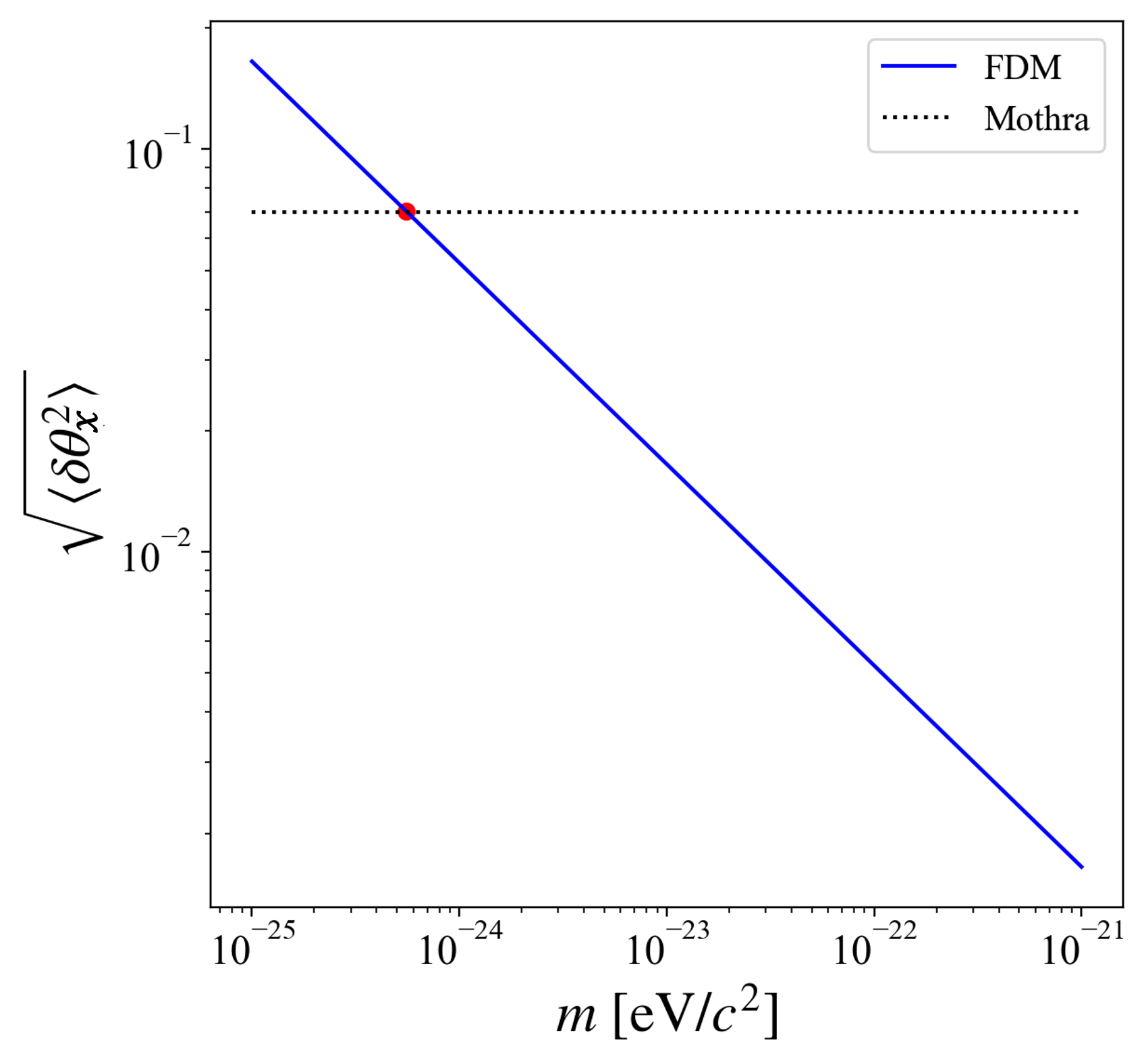
Figure 5: The relation between the critical curve perturbation and the FDM mass in the case of Mothra. The horizontal dotted line shows the fluctuation needed to explain the observed offset of Mothra.

V Conclusion

Astrometric perturbations of critical curves in strong lens systems serve as one of the most promising probes of small-scale substructures. A smooth mass distribution creates a geometry that yields multiple images with symmetric configurations around critical curves with radii of curvature about the Einstein radius. Substructures introduce small-scale fluctuations on the macro-critical curves created by smooth mass distributions, which indicates distortions or breaking the symmetry appearing in the macro-lens model. In this work, we have derived a general formula connecting fluctuations in the macro-critical curve with the fluctuations of the surface density due to substructures. This formula given in Eq. (16) allows us to analytically estimate the amplitude of the fluctuations from the surface density power spectrum of substructures.

We have explicitly checked the validity and accuracy of the formula in Eq. (16) using an open source code Glafic. Distributing subhalos near the macro-critical curve by the Poisson distribution, we have numerically computed critical curves with several models with different mass ranges of subhalos and calculated fluctuations of the macro-critical curves. We have found that our formula is indeed valid and accurate as long as substructures are not dominated by a small number of massive structures. The numerical results are summarized in Table 1.

As a demonstration of our analytic formula, we have explored the possibility that an extremely magnified binary star recently reported in Ref. [34] with JWST/NIRCam data, Mothra, can be explained by an unresolved magnified star whose position is offset due to the fluctuation of the macro-critical curve caused by substructures. We have found that CDM subhalos with masses ranging from $5\times 10^{7}~{}M_{\odot}/h$ to $10^{9}~{}M_{\odot}/h$ can well explain the anomalous position of Mothra. On the other hand, we have found that the FDM with a very small mass of $\sim 10^{-24}$ eV is needed to explain Mothra.

We expect that our analytic approach will be useful for studying fluctuations of macro-critical curve probed by highly magnified stars [29, 32] as well as by detailed mass modelling analysis of strong lensing systems [49, 50, 51, 52].

Appendix A The Fourier transformation of $\kappa$

The two-dimensional Fourier transformation of the two-dimensional surface density fluctuation is written by

$$\begin{split}\tilde{\kappa}_{\bm{k}}=\int d\bm{x}\kappa(\bm{x})e^{\-i\bm{k}\cdot\bm{x}}.\end{split}$$ (31)

$$\begin{split}\braket{\tilde{\kappa}_{\bm{k}}\tilde{\kappa}_{\bm{k}^{\prime}}}&=\int d\bm{x}\int d\bm{x}\prime~{}\braket{\kappa(\bm{x})\kappa(\bm{x}^{\prime})}e^{-i\bm{k}\cdot\bm{x}}e^{-i\bm{k}^{\prime}\cdot\bm{x}^{\prime}}\\ &\ =\int d\bm{X}\int d\bm{X}^{\prime}~{}\frac{1}{\Sigma_{\mathrm{cr}}^{2}}\braket{\rho(\bm{X})\rho(\bm{X}^{\prime})}e^{-i\bm{K}\cdot\bm{X}}e^{-i\bm{K}^{\prime}\cdot\bm{X}^{\prime}}|_{K_{Z}=K_{Z^{\prime}}=0}\\ &\ =\frac{1}{\Sigma_{\mathrm{cr}}^{2}}\int d\bm{X}\int d\bm{X}^{\prime}~{}e^{-i\bm{K}\cdot\bm{X}}e^{-i\bm{K}^{\prime}\cdot\bm{X}^{\prime}}\left\langle\sum_{i}m_{i}^{2}u(\bm{X}-\bm{X}_{i}|m)u(\bm{X}^{\prime}-\bm{X}_{i}|m)\right\rangle|_{K_{Z}=K_{Z^{\prime}}=0}\\ &\ =\frac{1}{\Sigma_{\mathrm{cr}}^{2}}\int d\bm{X}\int d\bm{X}^{\prime}\int d\bm{X}^{\prime\prime}\int dm~{}\frac{dn(\bm{X}^{\prime\prime})}{dm}m^{2}u(\bm{X}-\bm{X}^{\prime\prime}|m)u(\bm{X}^{\prime}-\bm{X}^{\prime\prime}|m)\\ &\ ~{}~{}~{}~{}~{}\times e^{-i\bm{K}\cdot(\bm{X}-\bm{X}^{\prime\prime})}e^{-i\bm{K}^{\prime}\cdot(\bm{X}^{\prime}-\bm{X}^{\prime\prime}))}e^{-i(\bm{K}+\bm{K}^{\prime})\cdot\bm{X}^{\prime\prime}}|_{K_{Z}=K_{Z^{\prime}}=0}\\ &\ =\frac{1}{\Sigma_{\mathrm{cr}}^{2}}\int d\bm{X}^{\prime\prime}~{}e^{-i(\bm{K}+\bm{K}^{\prime})\cdot\bm{X}^{\prime\prime}}\int dm~{}\frac{dn(\bm{X}^{\prime\prime})}{dm}m^{2}\tilde{u}_{\bm{K}}(m)\tilde{u}_{\bm{K}^{\prime}}(m)|_{K_{Z}=K_{Z^{\prime}}=0}\\ &\ =\frac{(2\pi)^{2}}{\Sigma_{\mathrm{cr}}^{2}}\int dZ^{\prime\prime}\int dm~{}\frac{dn(Z^{\prime\prime})}{dm}m^{2}\tilde{u}_{\bm{k}}(m)\tilde{u}_{\bm{k}^{\prime}}(m)\delta^{\mathrm{2D}}(\bm{k}+\bm{k}^{\prime})\\ &\ =(2\pi)^{2}\delta^{\mathrm{2D}}(\bm{k}+\bm{k}^{\prime})\frac{1}{\Sigma_{\mathrm{cr}}^{2}}\int dm~{}\frac{dn^{\mathrm{2D}}}{dm}m^{2}\tilde{u}_{\bm{k}}(m)\tilde{u}_{\bm{k}^{\prime}}(m),\end{split}$$ (32)

where $\bm{x}$ and $\bm{X}$ are two- and three-dimensional coordinates, respectively, $\bm{k}=(k_{x},k_{y})$, $\bm{K}=(k_{x},k_{y},K_{z})$, and we assume that the spatial correlations among subhalos can be neglected. We also assume that the subhalo number density depends only on the coordinate along the line of sight, i.e. redshift. In this equation, we denote

$$\begin{split}\tilde{u}_{\bm{K}}|_{K_{z}=0}=\tilde{u}_{\bm{k}}.\end{split}$$ (33)

On the other hand, we can calculate $\braket{\tilde{\kappa}_{\bm{k}}\tilde{\kappa}_{\bm{k}^{\prime}}}$ directly like

$$\begin{split}\braket{\tilde{\kappa}_{\bm{k}}\tilde{\kappa}_{\bm{k}^{\prime}}}&=\int d\bm{x}\int d\bm{x}\prime~{}\braket{\kappa(\bm{x})\kappa(\bm{x}^{\prime})}e^{-i\bm{k}\cdot\bm{x}}e^{-i\bm{k}^{\prime}\cdot\bm{x}^{\prime}}\\ &\ =\frac{1}{\Sigma_{\mathrm{cr}}^{2}}\int d\bm{x}\int d\bm{x}^{\prime}~{}\int d\bm{x}^{\prime\prime}\int dm\frac{dn^{\mathrm{2D}}}{dm}m^{2}u^{\mathrm{2D}}(\bm{x}-\bm{x}^{\prime\prime}|m)u^{\mathrm{2D}}(\bm{x}^{\prime}-\bm{x}^{\prime\prime}|m)\\ &\ ~{}~{}~{}~{}~{}\times e^{-i\bm{k}\cdot(\bm{x}-\bm{x}^{\prime\prime})}e^{-i\bm{k}^{\prime}\cdot(\bm{x}^{\prime}-\bm{x}^{\prime\prime})}e^{-i(\bm{k}+\bm{k}^{\prime})\cdot\bm{x}^{\prime\prime}}\\ &\ =(2\pi)^{2}\delta(\bm{k}+\bm{k}^{\prime})\frac{1}{\Sigma_{\mathrm{cr}}^{2}}\int dm\frac{dn^{\mathrm{2D}}}{dm}m^{2}\tilde{u}^{\mathrm{2D}}_{\bm{k}}(m)\tilde{u}^{\mathrm{2D}}_{\bm{k}^{\prime}}(m).\end{split}$$ (34)

Then one can find that $u_{\bm{k}}$ represented in Eq. (33) is actually the two-dimensional Fourier transformation of the two-dimensional (normalized) surface density profile.

References

- Reid et al. [2010] B. A. Reid, W. J. Percival, D. J. Eisenstein, L. Verde, D. N. Spergel, R. A. Skibba, N. A. Bahcall, T. Budavari, J. A. Frieman, M. Fukugita, J. R. Gott, J. E. Gunn, Ž. Ivezić, G. R. Knapp, R. G. Kron, R. H. Lupton, T. A. McKay, A. Meiksin, R. C. Nichol, A. C. Pope, D. J. Schlegel, D. P. Schneider, C. Stoughton, M. A. Strauss, A. S. Szalay, M. Tegmark, M. S. Vogeley, D. H. Weinberg, D. G. York, and I. Zehavi, Cosmological constraints from the clustering of the Sloan Digital Sky Survey DR7 luminous red galaxies, MNRAS 404, 60 (2010), arXiv:0907.1659 [astro-ph.CO] .
- Chabanier et al. [2019a] S. Chabanier, N. Palanque-Delabrouille, C. Yèche, J.-M. Le Goff, E. Armengaud, J. Bautista, M. Blomqvist, N. Busca, K. Dawson, T. Etourneau, A. Font-Ribera, Y. Lee, H. du Mas des Bourboux, M. Pieri, J. Rich, G. Rossi, D. Schneider, and A. Slosar, The one-dimensional power spectrum from the SDSS DR14 Ly forests, J. Cosmology Astropart. Phys 2019, 017 (2019a), arXiv:1812.03554 [astro-ph.CO] .
- Chabanier et al. [2019b] S. Chabanier, M. Millea, and N. Palanque-Delabrouille, Matter power spectrum: from Ly forest to CMB scales, MNRAS 489, 2247 (2019b), arXiv:1905.08103 [astro-ph.CO] .
- Planck Collaboration [2020] Planck Collaboration, Planck 2018 results. VI. Cosmological parameters, A&A 641, A6 (2020), arXiv:1807.06209 [astro-ph.CO] .
- Del Popolo and Le Delliou [2017] A. Del Popolo and M. Le Delliou, Small Scale Problems of the CDM Model: A Short Review, Galaxies 5, 17 (2017), arXiv:1606.07790 [astro-ph.CO] .
- Bullock and Boylan-Kolchin [2017] J. S. Bullock and M. Boylan-Kolchin, Small-Scale Challenges to the CDM Paradigm, ARA&A 55, 343 (2017), arXiv:1707.04256 [astro-ph.CO] .
- Colín et al. [2000] P. Colín, V. Avila-Reese, and O. Valenzuela, Substructure and Halo Density Profiles in a Warm Dark Matter Cosmology, ApJ 542, 622 (2000), arXiv:astro-ph/0004115 [astro-ph] .
- Bode et al. [2001] P. Bode, J. P. Ostriker, and N. Turok, Halo Formation in Warm Dark Matter Models, ApJ 556, 93 (2001), arXiv:astro-ph/0010389 [astro-ph] .
- Viel et al. [2005] M. Viel, J. Lesgourgues, M. G. Haehnelt, S. Matarrese, and A. Riotto, Constraining warm dark matter candidates including sterile neutrinos and light gravitinos with WMAP and the Lyman- forest, Phys. Rev. D 71, 063534 (2005), arXiv:astro-ph/0501562 [astro-ph] .
- Peebles [2000] P. J. E. Peebles, Fluid Dark Matter, ApJ 534, L127 (2000), arXiv:astro-ph/0002495 [astro-ph] .
- Hu et al. [2000] W. Hu, R. Barkana, and A. Gruzinov, Fuzzy Cold Dark Matter: The Wave Properties of Ultralight Particles, Phys. Rev. Lett. 85, 1158 (2000), arXiv:astro-ph/0003365 [astro-ph] .
- Schive et al. [2014] H.-Y. Schive, M.-H. Liao, T.-P. Woo, S.-K. Wong, T. Chiueh, T. Broadhurst, and W.-Y. P. Hwang, Understanding the core-halo relation of quantum wave dark matter from 3d simulations, Phys. Rev. Lett. 113, 261302 (2014).
- Hui et al. [2017] L. Hui, J. P. Ostriker, S. Tremaine, and E. Witten, Ultralight scalars as cosmological dark matter, Phys. Rev. D 95, 043541 (2017), arXiv:1610.08297 [astro-ph.CO] .
- Moore et al. [1999] B. Moore, S. Ghigna, F. Governato, G. Lake, T. Quinn, J. Stadel, and P. Tozzi, Dark Matter Substructure within Galactic Halos, ApJ 524, L19 (1999), arXiv:astro-ph/9907411 [astro-ph] .
- Mao and Schneider [1998] S. Mao and P. Schneider, Evidence for substructure in lens galaxies?, MNRAS 295, 587 (1998), arXiv:astro-ph/9707187 [astro-ph] .
- Metcalf and Madau [2001] R. B. Metcalf and P. Madau, Compound Gravitational Lensing as a Probe of Dark Matter Substructure within Galaxy Halos, ApJ 563, 9 (2001), arXiv:astro-ph/0108224 [astro-ph] .
- Chiba [2002] M. Chiba, Probing Dark Matter Substructure in Lens Galaxies, ApJ 565, 17 (2002), arXiv:astro-ph/0109499 [astro-ph] .
- Metcalf and Zhao [2002] R. B. Metcalf and H. Zhao, Flux Ratios as a Probe of Dark Substructures in Quadruple-Image Gravitational Lenses, ApJ 567, L5 (2002), arXiv:astro-ph/0111427 [astro-ph] .
- Dalal and Kochanek [2002] N. Dalal and C. S. Kochanek, Direct Detection of Cold Dark Matter Substructure, ApJ 572, 25 (2002), arXiv:astro-ph/0111456 [astro-ph] .
- Bradač et al. [2002] M. Bradač, P. Schneider, M. Steinmetz, M. Lombardi, L. J. King, and R. Porcas, B1422+231: The influence of mass substructure on strong lensing, A&A 388, 373 (2002), arXiv:astro-ph/0112038 [astro-ph] .
- Metcalf and Amara [2012] R. B. Metcalf and A. Amara, Small-scale structures of dark matter and flux anomalies in quasar gravitational lenses, MNRAS 419, 3414 (2012), arXiv:1007.1599 [astro-ph.CO] .
- Nierenberg et al. [2017] A. M. Nierenberg, T. Treu, G. Brammer, A. H. G. Peter, C. D. Fassnacht, C. R. Keeton, C. S. Kochanek, K. B. Schmidt, D. Sluse, and S. A. Wright, Probing dark matter substructure in the gravitational lens HE 0435-1223 with the WFC3 grism, MNRAS 471, 2224 (2017), arXiv:1701.05188 [astro-ph.CO] .
- Gilman et al. [2020] D. Gilman, S. Birrer, A. Nierenberg, T. Treu, X. Du, and A. Benson, Warm dark matter chills out: constraints on the halo mass function and the free-streaming length of dark matter with eight quadruple-image strong gravitational lenses, MNRAS 491, 6077 (2020), arXiv:1908.06983 [astro-ph.CO] .
- Hsueh et al. [2019] J.-W. Hsueh, W. Enzi, S. Vegetti, M. W. Auger, C. D. Fassnacht, G. Despali, L. V. E. Koopmans, and J. P. McKean, SHARP – VII. New constraints on the dark matter free-streaming properties and substructure abundance from gravitationally lensed quasars, Monthly Notices of the Royal Astronomical Society 492, 3047 (2019), https://academic.oup.com/mnras/article-pdf/492/2/3047/43927118/stz3177.pdf .
- Hezaveh et al. [2013] Y. Hezaveh, N. Dalal, G. Holder, M. Kuhlen, D. Marrone, N. Murray, and J. Vieira, Dark Matter Substructure Detection Using Spatially Resolved Spectroscopy of Lensed Dusty Galaxies, ApJ 767, 9 (2013), arXiv:1210.4562 [astro-ph.CO] .
- Hezaveh et al. [2016] Y. Hezaveh, N. Dalal, G. Holder, T. Kisner, M. Kuhlen, and L. Perreault Levasseur, Measuring the power spectrum of dark matter substructure using strong gravitational lensing, J. Cosmology Astropart. Phys 2016, 048 (2016), arXiv:1403.2720 [astro-ph.CO] .
- Birrer et al. [2017] S. Birrer, A. Amara, and A. Refregier, Lensing substructure quantification in RXJ1131-1231: a 2 keV lower bound on dark matter thermal relic mass, J. Cosmology Astropart. Phys 2017, 037 (2017), arXiv:1702.00009 [astro-ph.CO] .
- Asadi et al. [2017] S. Asadi, E. Zackrisson, and E. Freeland, Probing cold dark matter subhaloes with simulated ALMA observations of macrolensed sub-mm galaxies, MNRAS 472, 129 (2017), arXiv:1709.00729 [astro-ph.GA] .
- Dai et al. [2018] L. Dai, T. Venumadhav, A. A. Kaurov, and J. Miralda-Escud, Probing Dark Matter Subhalos in Galaxy Clusters Using Highly Magnified Stars, ApJ 867, 24 (2018), arXiv:1804.03149 [astro-ph.CO] .
- Kelly et al. [2018] P. L. Kelly, J. M. Diego, S. Rodney, N. Kaiser, T. Broadhurst, A. Zitrin, T. Treu, P. G. Pérez-González, T. Morishita, M. Jauzac, J. Selsing, M. Oguri, L. Pueyo, T. W. Ross, A. V. Filippenko, N. Smith, J. Hjorth, S. B. Cenko, X. Wang, D. A. Howell, J. Richard, B. L. Frye, S. W. Jha, R. J. Foley, C. Norman, M. Bradac, W. Zheng, G. Brammer, A. M. Benito, A. Cava, L. Christensen, S. E. de Mink, O. Graur, C. Grillo, R. Kawamata, J.-P. Kneib, T. Matheson, C. McCully, M. Nonino, I. Pérez-Fournon, A. G. Riess, P. Rosati, K. B. Schmidt, K. Sharon, and B. J. Weiner, Extreme magnification of an individual star at redshift 1.5 by a galaxy-cluster lens, Nature Astronomy 2, 334 (2018), arXiv:1706.10279 [astro-ph.GA] .
- Welch et al. [2022] B. Welch, D. Coe, J. M. Diego, A. Zitrin, E. Zackrisson, P. Dimauro, Y. Jiménez-Teja, P. Kelly, G. Mahler, M. Oguri, F. X. Timmes, R. Windhorst, M. Florian, S. E. de Mink, R. J. Avila, J. Anderson, L. Bradley, K. Sharon, A. Vikaeus, S. McCandliss, M. Bradač, J. Rigby, B. Frye, S. Toft, V. Strait, M. Trenti, S. Sharma, F. Andrade-Santos, and T. Broadhurst, A highly magnified star at redshift 6.2, Nature 603, 815 (2022), arXiv:2209.14866 [astro-ph.GA] .
- Williams et al. [2023] L. L. R. Williams, P. L. Kelly, T. Treu, A. Amruth, J. M. Diego, S. Kei Li, A. K. Meena, A. Zitrin, and T. J. Broadhurst, Flashlights: Properties of Highly Magnified Images Near Cluster Critical Curves in the Presence of Dark Matter Subhalos, arXiv e-prints , arXiv:2304.06064 (2023), arXiv:2304.06064 [astro-ph.CO] .
- Kawai et al. [2022] H. Kawai, M. Oguri, A. Amruth, T. Broadhurst, and J. Lim, An Analytic Model for the Subgalactic Matter Power Spectrum in Fuzzy Dark Matter Halos, ApJ 925, 61 (2022), arXiv:2109.04704 [astro-ph.CO] .
- Diego et al. [2023] J. M. Diego, B. Sun, H. Yan, L. J. Furtak, E. Zackrisson, L. Dai, P. Kelly, M. Nonino, N. Adams, A. K. Meena, S. P. Willner, A. Zitrin, S. H. Cohen, J. C. J. D. Silva, R. A. Jansen, J. Summers, R. A. Windhorst, D. Coe, C. J. Conselice, S. P. Driver, B. Frye, N. A. Grogin, A. M. Koekemoer, M. A. Marshall, N. Pirzkal, A. Robotham, M. J. Rutkowski, J. Ryan, Russell E., S. Tompkins, C. N. A. Willmer, and R. Bhatawdekar, JWST’s PEARLS: Mothra, a new kaiju star at z=2.091 extremely magnified by MACS0416, and implications for dark matter models, arXiv e-prints , arXiv:2307.10363 (2023), arXiv:2307.10363 [astro-ph.CO] .
- Blandford and Narayan [1986] R. Blandford and R. Narayan, Fermat’s Principle, Caustics, and the Classification of Gravitational Lens Images, ApJ 310, 568 (1986).
- Cooray and Sheth [2002] A. Cooray and R. Sheth, Halo models of large scale structure, Phys. Rep. 372, 1 (2002), arXiv:astro-ph/0206508 [astro-ph] .
- Navarro et al. [1996] J. F. Navarro, C. S. Frenk, and S. D. M. White, The Structure of Cold Dark Matter Halos, ApJ 462, 563 (1996), arXiv:astro-ph/9508025 [astro-ph] .
- Scoccimarro et al. [2001] R. Scoccimarro, R. K. Sheth, L. Hui, and B. Jain, How Many Galaxies Fit in a Halo? Constraints on Galaxy Formation Efficiency from Spatial Clustering, ApJ 546, 20 (2001), arXiv:astro-ph/0006319 [astro-ph] .
- Ishiyama and Ando [2020] T. Ishiyama and S. Ando, The abundance and structure of subhaloes near the free streaming scale and their impact on indirect dark matter searches, MNRAS 492, 3662 (2020), arXiv:1907.03642 [astro-ph.CO] .
- Nakamura and Suto [1997] T. T. Nakamura and Y. Suto, Strong Gravitational Lensing and Velocity Function as Tools to Probe Cosmological Parameters: Current Constraints and Future Predictions, Progress of Theoretical Physics 97, 49 (1997), https://academic.oup.com/ptp/article-pdf/97/1/49/5231233/97-1-49.pdf .
- Diemer and Kravtsov [2015] B. Diemer and A. V. Kravtsov, A Universal Model for Halo Concentrations, ApJ 799, 108 (2015), arXiv:1407.4730 [astro-ph.CO] .
- Oguri and Takahashi [2020] M. Oguri and R. Takahashi, Probing Dark Low-mass Halos and Primordial Black Holes with Frequency-dependent Gravitational Lensing Dispersions of Gravitational Waves, ApJ 901, 58 (2020), arXiv:2007.01936 [astro-ph.CO] .
- Oguri [2010] M. Oguri, The Mass Distribution of SDSS J1004+4112 Revisited, PASJ 62, 1017 (2010), arXiv:1005.3103 [astro-ph.CO] .
- Oguri [2021] M. Oguri, Fast Calculation of Gravitational Lensing Properties of Elliptical Navarro-Frenk-White and Hernquist Density Profiles, PASP 133, 074504 (2021), arXiv:2106.11464 [astro-ph.IM] .
- Umetsu et al. [2014] K. Umetsu, E. Medezinski, M. Nonino, J. Merten, M. Postman, M. Meneghetti, M. Donahue, N. Czakon, A. Molino, S. Seitz, D. Gruen, D. Lemze, I. Balestra, N. Benítez, A. Biviano, T. Broadhurst, H. Ford, C. Grillo, A. Koekemoer, P. Melchior, A. Mercurio, J. Moustakas, P. Rosati, and A. Zitrin, CLASH: Weak-lensing Shear-and-magnification Analysis of 20 Galaxy Clusters, ApJ 795, 163 (2014), arXiv:1404.1375 .
- Kawamata et al. [2016] R. Kawamata, M. Oguri, M. Ishigaki, K. Shimasaku, and M. Ouchi, Precise Strong Lensing Mass Modeling of Four Hubble Frontier Field Clusters and a Sample of Magnified High-redshift Galaxies, ApJ 819, 114 (2016), arXiv:1510.06400 [astro-ph.GA] .
- Behroozi et al. [2019] P. Behroozi, R. H. Wechsler, A. P. Hearin, and C. Conroy, UNIVERSEMACHINE: The correlation between galaxy growth and dark matter halo assembly from z = 0-10, MNRAS 488, 3143 (2019), arXiv:1806.07893 [astro-ph.GA] .
- Hernquist [1990] L. Hernquist, An Analytical Model for Spherical Galaxies and Bulges, ApJ 356, 359 (1990).
- Dai et al. [2020] L. Dai, A. A. Kaurov, K. Sharon, M. Florian, J. Miralda-Escudé, T. Venumadhav, B. Frye, J. R. Rigby, and M. Bayliss, Asymmetric surface brightness structure of caustic crossing arc in SDSS J1226+2152: a case for dark matter substructure, MNRAS 495, 3192 (2020), arXiv:2001.00261 [astro-ph.GA] .
- Amruth et al. [2023] A. Amruth, T. Broadhurst, J. Lim, M. Oguri, G. F. Smoot, J. M. Diego, E. Leung, R. Emami, J. Li, T. Chiueh, H.-Y. Schive, M. C. H. Yeung, and S. K. Li, Einstein rings modulated by wavelike dark matter from anomalies in gravitationally lensed images, Nature Astronomy 7, 736 (2023), arXiv:2304.09895 [astro-ph.CO] .
- Inoue et al. [2023] K. T. Inoue, T. Minezaki, S. Matsushita, and K. Nakanishi, ALMA Measurement of 10 kpc Scale Lensing-power Spectra toward the Lensed Quasar MG J0414+0534, ApJ 954, 197 (2023), arXiv:2109.01168 [astro-ph.CO] .
- Powell et al. [2023] D. M. Powell, S. Vegetti, J. P. McKean, S. D. M. White, E. G. M. Ferreira, S. May, and C. Spingola, A lensed radio jet at milli-arcsecond resolution - II. Constraints on fuzzy dark matter from an extended gravitational arc, MNRAS 524, L84 (2023), arXiv:2302.10941 [astro-ph.CO] .