Distributed Adaptive Greedy Quasi-Newton Methods with Explicit Non-asymptotic Convergence Bounds

Abstract

Though quasi-Newton methods have been extensively studied in the literature, they either suffer from local convergence or use a series of line searches for global convergence which is not acceptable in the distributed setting. In this work, we first propose a line search free greedy quasi-Newton (GQN) method with adaptive steps and establish explicit non-asymptotic bounds for both the global convergence rate and local superlinear rate. Our novel idea lies in the design of multiple greedy quasi-Newton updates, which involves computing Hessian-vector products, to control the Hessian approximation error, and a simple mechanism to adjust stepsizes to ensure the objective function improvement per iterate. Then, we extend it to the master-worker framework and propose a distributed adaptive GQN method whose communication cost is comparable with that of first-order methods, yet it retains the superb convergence property of its centralized counterpart. Finally, we demonstrate the advantages of our methods via numerical experiments.

,

[cor]Corresponding author

1 Introduction

Quasi-Newton methods contain a popular class of optimization algorithms where the exact Hessian in the Newton method is iteratively approximated, and have been extensively studied for quite a long history (Nocedal and Wright, 2006). Though they retain the superlinear convergence property of Newton methods near the optimal solution, they either suffer from local convergence with a small domain or require a series of line searches for global convergence whose number of searches per iterate is unpredictable.

Recently, Polyak and Tremba (2020) proposes a novel procedure for directly adjusting stepsizes in Newton methods to achieve a wide range of convergence (even globally) and local quadratic convergence. Unfortunately, such an adaptive idea cannot be directly applied to the quasi-Newton methods (e.g., DFP, BFGS, SR1) as their Hessian approximation errors cannot be evaluated or controlled. In this work, we adopt the greedy quasi-Newton (GQN) update in Rodomanov and Nesterov (2021a) which is a variant of the Broyden family with the greedily selected vectors to maximize a certain measure of progress and involves computing Hessian-vector products (HVPs). To ensure global convergence, we propose to use multiple GQN updates to uniformly bound the Hessian approximation errors, and then design a new simple mechanism to adaptively adjust stepsizes, leading to the line search free AGQN of this work. Under the strongly convex objective function with Lipschitz continuous Hessian, we derive explicit non-asymptotic bounds for both the global convergence rate and local superlinear rate. It is worthy mentioning that even for quasi-Newton methods, the (local) non-asymptotic convergence has been unknown until very recently (Rodomanov and Nesterov, 2022; Jin and Mokhtari, 2022; Rodomanov and Nesterov, 2021b). Our AGQN is the first QN method that is line search free and achieves global convergence with local superlinear rates.

Next, we extend to the distributed master-worker setting where the master updates the decision vector by using information from all workers. Though the distributed method can significantly accelerate the centralized one, how to fully explore the potential of second-order methods in the distributed setting largely remains open. One of the major bottlenecks lies in that any worker cannot compute the QN direction by itself and has to use information from other workers. This is in sharp contrast to the first-order methods where each worker independently computes its gradient direction in parallel, and thus it is relatively easy to achieve speed-up property.

A natural idea is that the worker only transmits a limited number of vectors to form the Hessian estimate or the QN direction. We propose a divide-and-combine strategy to ensure that each worker only sends a vector of dimension $O((\tau+1)n)$ per iterate to the master where $n$ is the dimension of decision vector and the integer valued $\tau\ll n$ is newly introduced to ensure global convergence. Noticeably, $\tau$ can be as small as one, and even zero if the algorithm enters the local region of superlinear convergence, which can be explicit in practice. From this perspective, the communication complexity per iterate is comparable to that of the first-order method in the master-worker setting. Yet our distributed method, namely DAGQN, not only retains the superb convergence property of the AGQN with non-asymptotic convergence bounds, but also is line search free. Specifically, we first divide the task of approximating Hessian among all workers, i.e., let each worker $i$ perform GQN updates to approximate its individual local Hessian and extracts the required vector for the GQN update to transmit to the master in a single packet. Since the master can reconstruct the same copies of local Hessian estimates, it simply aggregates them to compute the QN direction. Besides the low communication complexity, we are still able to establish explicit non-asymptotic bounds for both the global convergence rate and local superlinear rate for our distributed GQN method.

Many efforts have been made to reduce the communication cost for the distributed setting. For example, each worker in NL (Islamov et al., 2021) and FedNL (Safaryan et al., 2022) dynamically learns the Hessian at the optimum and sends compressed shift term to the master. Agafonov et al. (2022) builds upon FedNL with a more computation and memory efficient scheme. GIANT (Wang et al., 2018) learns the Newton direction via the harmonic mean of local Newton directions from workers, and each worker in DANE (Shamir et al., 2014) sends a solution vector of a local subproblem to the master. DINGO (Crane and Roosta, 2019) and DINO (Crane and Roosta, 2020) find descent directions by combining local Newton directions from workers. Fabbro et al. (2022) approximates Hessian with its principal eigenvectors, and transmits them in an incremental and sporadic manner to amortize the communication cost. Alimisis et al. (2021) vectorizes Hessian and performs lattice-based quantization before communication. DAve-QN (Soori et al., 2020) approximates Hessian with the classical BFGS but implements it using an asynchronous scheme. In comparison, our DAGQN has at least two sharp differences: (a) it only involves computing HVPs for updating, instead of explicitly computing Hessian or solving a subproblem per iteration. (b) The global convergence is achieved via adaptively tuning stepsize without line search and the local convergence has explicit superlinear rates.

Note that there are also distributed second-order methods for peer-to-peer networks, e.g., DAN-LA (Zhang et al., 2022) estimates the Hessian via an outer product of a moderate number of vectors that are obtained via the low-rank matrix approximation. And the decentralized BFGS method in Eisen et al. (2017) has a linear rate. See Mokhtari et al. (2016); Eisen et al. (2017); Lee et al. (2018); Tutunov et al. (2019); Soori et al. (2020); Mansoori and Wei (2020); Li et al. (2021, 2022); Zhang et al. (2022).

Finally, we adopt a logistic regression problem with real datasets to validate the advantages of our proposed methods. Numerical results validate that both AGQN and its distributed version are quite competitive for problems where HVPs can be efficiently computed. Overall, contributions of this work can be summarized as follows:

1. Our AGQN is the first QN method that is not only line search free, but also achieves global convergence and local superlinear convergence with explicit non-asymptotic bounds.

2. The AGQN is extended to the master-worker setting with a low communication complexity that is comparable to that of distributed first-order methods. Yet, it retains the superb convergence property of the AGQN.

The rest of this paper is organized as follows. In Section 2, we briefly review the GQN method. In Section 3, we propose the AGQN method and study its convergence. It should be noted that the preliminary results of this section have been presented in Du and You (2022). In Section 4 and 5, we propose the distributed AGQN method and conduct convergence analysis, respectively. In Section 6, we perform simulations to validate the performance of our methods.

Notation: $\|\cdot\|$ is the standard Euclidean norm, and $\langle\cdot,\cdot\rangle$ is the standard inner product in $\mathbb{R}^{n}$. For a twice differentiable function $f:\mathbb{R}^{n}\rightarrow\mathbb{R}$, denote its gradient and Hessian as $\nabla f$ and $\nabla^{2}f$, respectively. For a symmetric matrix $A$, denote $A\succ 0$ $(A\succeq 0)$ if $A$ is positive (semi-)definite. Given $A\succeq 0$ and $B\succeq 0$, the relation $A\succeq B$ means that $A-B\succeq 0$ and $\langle A,B\rangle=\textrm{Trace}(AB).$ For simplicity, we write $\|h\|_{A}=\langle Ah,h\rangle^{1/2}$ and $\|h\|_{A}^{*}=\langle A^{-1}h,h\rangle^{1/2},\forall h\in\mathbb{R}^{n}.$ For simplicity, we omit the iteration index $k$ and use $x$, $x^{-}$, $x^{+}$ to represent $x^{k}$, $x^{k-1}$, $x^{k+1}$, respectively. Similar notation will be applied to other vectors and variables.

2 The basics of greedy quasi-Newton and our objective

In this section, we review some basics of the greedy quasi-Newton (GQN) method in Rodomanov and Nesterov (2021a). In the literature, three QN methods have been widely used, see e.g., Nocedal and Wright (2006). Given symmetric positive definite matrices $A,G\in\mathbb{R}^{n\times n}$ and a vector $u\in\mathbb{R}^{n}$, satisfying that $G\succeq A$ and $Gu\neq Au$, the SR1 update is

$$\textrm{SR1}(G,A,u)=G-\frac{(G-A)uu^{\mathsf{T}}(G-A)}{\langle(G-A)u,u\rangle}$$ (1)

where $u\in\mathbb{R}^{n}$, and the DFP update is given by

$$\textrm{DFP}(G,A,u)={} G-\frac{Auu^{\mathsf{T}}G+Guu^{\mathsf{T}}A}{\langle Au,u\rangle}$$ (2)

$$+\left(\frac{\langle Gu,u\rangle}{\langle Au,u\rangle}+1\right)\frac{Auu^{\mathsf{T}}A}{\langle Au,u\rangle}.$$

A convex combination of the SR1 and the DFP leads to the celebrated Broyden family

$$\textrm{Broyd}(G,A,u)=$$ (3)

$$~{}~{}~{}~{}~{}~{}~{}~{}~{}~{}~{}~{}\phi\textrm{DFP}(G,A,u)+(1-\phi)\textrm{SR1}(G,A,u)$$

where $\phi$ can be chosen any value from $[0,1]$ at every call of (LABEL:equ:broyden_update_formula). Let $\phi={\langle Au,u\rangle}{\langle Gu,u\rangle}^{-1}\in(0,1]$, it reduces to the BFGS update

$$\textrm{BFGS}(G,A,u)=G-\frac{Guu^{\mathsf{T}}G}{\langle Gu,u\rangle}+\frac{Auu^{\mathsf{T}}A}{\langle Au,u\rangle}.$$ (4)

In the optimization progress, we use Broyd to update the estimate of the Hessian matrix via two vectors $u$ and $Au$, and thus avoid directly computing the Hessian matrix. If $A=\nabla^{2}f$, then the Hessian-vector product (HVP) $Au$ can be computed as a whole with similar computational efforts as that of $\nabla f$ Pearlmutter (1994). We use the following example to illustrate this point.

Example 1.

In applications, we usually require to solve empirical risk problems (ERP) in the form of the following generalized linear model (GLM)

$$\varphi(x)=\sum_{i=1}^{m}\varphi_{i}(a_{i}^{\mathsf{T}}x)$$ (5)

where $x\in\mathbb{R}^{n}$, $\varphi_{i}$ is a twice differentiable function and $a_{i}$ is a training sample. In the GLM, it is trivial that

$$\nabla\varphi(x)=\sum_{i=1}^{m}\varphi^{\prime}_{i}(a_{i}^{\mathsf{T}}x)a_{i},\ \ \nabla^{2}\varphi(x)=\sum_{i=1}^{m}\varphi^{\prime\prime}_{i}(a_{i}^{\mathsf{T}}x)a_{i}a_{i}^{\mathsf{T}}$$ (6)

$$\nabla^{2}\varphi(x)u=\sum_{i=1}^{m}\varphi_{i}^{\prime\prime}(a_{i}^{\mathsf{T}}x)a_{i}(a_{i}^{\mathsf{T}}u).$$

The computational complexities of $\nabla\varphi(x)$ and the HVP $\nabla^{2}\varphi(x)u$ are of the same as $O(nm)$, while the complexity of $\nabla^{2}\varphi(x)$ is $O(n^{2}m)$.∎

If we select $u$ in (LABEL:equ:broyden_update_formula) greedily from the standard unit vectors of $\mathbb{R}^{n}$, i.e.,

$$g_{A}(G)=\underset{u\in\{e_{1},\ldots,e_{n}\}}{\operatorname*{\text{argmax}}}\frac{\langle Gu,u\rangle}{\langle Au,u\rangle},$$ (7)

the GQN update is iteratively given by

$$G^{k+1} =\textrm{Broyd}(G^{k},A,g_{A}(G^{k}))$$ (8)

$$\overset{\textrm{def}}{=}\textrm{gBroyd}(G^{k},A).$$

A striking feature of the GQN is that we are able to explicitly evaluate the convergence rate of $\{G^{k}\}$ to $A$ via the following metric

$$\sigma_{A}(G)=\langle A^{-1},G-A\rangle=\langle A^{-1},G\rangle-n$$ (9)

where $n$ is the dimension of the vector space.

Lemma 1 (Rodomanov and Nesterov (2021a)).

If $0\prec\mu I\preceq A\preceq\omega I$ and $G^{k}\succeq A$ in (8), then

$$\sigma_{A}(G^{k+1})\leq(1-\mu/(n\omega))\sigma_{A}(G^{k}).$$ (10)

Under suitable conditions, the GQN method using a correction strategy has been shown to achieve a local explicit superlinear rate in Rodomanov and Nesterov (2021a). In this work, we design an adaptive GQN method to achieve global convergence in Section 3 and extend it to the master-worker setting in Section 4. Both can also achieve local linear and superlinear convergence. Moreover, the communication complexity of the distributed version is comparable to that of distributed first-order methods.

3 The adaptive greedy quasi-Newton method in the centralized setting

In this section, we first propose a novel adaptive GQN (AGQN) method where a simple mechanism is designed to adaptively adjust stepsizes to ensure its global convergence. Our key idea lies in the use of Lemma 1 to adaptively tune stepsizes to uniformly bound the Hessian approximation error. Then, we establish explicit non-asymptotic bounds for both the global convergence rate and local superlinear rate of the AGQN.

Consider an unconstrained optimization problem

$$\underset{x\in\mathbb{R}^{n}}{\operatorname*{minimize}}\ \ f(x).$$ (11)

Suppose that $x$ is the current iterate and $G\succ 0$ is an estimate of $\nabla^{2}f(x)$. A generic QN method has the following form

$$x^{+}=x-\alpha\cdot G^{-1}\nabla f(x)$$ (12)

where $0<\alpha\leq 1$ is the stepsize and $f$ satisfies the following condition.

Assumption 2.

1. $f$ is $\mu$-strongly convex and $\omega$-smooth, i.e.,

   $$\mu I\preceq\nabla^{2}f(x)\preceq\omega I,\forall x\in\mathbb{R}^{n}$$ (13)

   in which case we denote its condition number by $\kappa=\omega/\mu$.

2. The Hessian of $f$ is $L$-Lipschitz continuous:

   $$\|\nabla^{2}f(y)-\nabla^{2}f(x)\|\leq L\|y-x\|,\forall x,y\in\mathbb{R}^{n}.$$ (14)

Under Assumption 2, one can establish the so-called strong self-concordancy of $f$.

Lemma 3.

(Rodomanov and Nesterov (2021a)) Suppose that $f(x)$ satisfies Assumption 2. Then $f(x)$ is strongly self-concordant with a constant $M\leq L/\mu^{3/2}>0$, i.e., for all $x,y,z,w\in\mathbb{R}^{n}$, it holds that

$$\nabla^{2}f(y)-\nabla^{2}f(x)\preceq M\|y-x\|_{\nabla^{2}f(z)}\nabla^{2}f(w).$$ (15)

For convenience we shall directly use $M$ as the constant of strong self-concordancy in the sequel. Assumption 2 is common in the analysis of Newton-type methods (Polyak and Tremba, 2020; Boyd and Vandenberghe, 2004). Note that the strong self-concordancy is the key for the correction strategy to Rodomanov and Nesterov (2021a).

3.1 Adaptive stepsizes for the global uniform boundedness of Hessian estimate errors

The key idea for our AGQN is that the Hessian approximation error can be explicitly bounded in the optimization progress. Specifically, suppose that $G\succeq\nabla^{2}f(x)$ is a “good” approximation of $\nabla^{2}f(x)$, i.e., there exists a small constant $\varepsilon\geq 0$ such that

$$\sigma_{\nabla^{2}f(x)}(G)\leq\varepsilon.$$ (16)

To approximate $\nabla^{2}f(x^{+})$, a corrected $G$ is employed in the GQN, i.e.,

$$\overline{G}^{+}=(1+Mr^{+})G,~{}\textrm{and~{}}G^{+}=\textrm{gBroyd}(\overline{G}^{+},\nabla^{2}f(x^{+}))\\$$ (17)

where gBroyd is defined in (8) and

$$r^{+}=\|x^{+}-x\|_{\nabla^{2}f(x)}.$$ (18)

Note that $r^{+}$ can also be efficiently computed by the HVP (see Example 1). Such a correction strategy is essential as it not only ensures an upper Hessian estimate but also the error can be evaluated. Specifically, it follows from Rodomanov and Nesterov (2021a, Lemma 4.8) that

$$\sigma_{\nabla^{2}f(x^{+})}(G^{+})$$ (19)

$$\leq\left(1-\frac{1}{n\kappa}\right)(1+Mr^{+})^{2}\left(\varepsilon+\frac{2nMr^{+}}{1+Mr^{+}}\right).$$

Apparently, the Hessian approximation error at $x^{+}$ grows as $r^{+}$ increases. In the global analysis where $x$ can be arbitrarily far away from the optimal solution, we cannot bound $r^{+}$ and thus the Hessian approximation error is not restricted, which is the main challenge to establish global convergence for the GQN method.

To resolve it, we propose to use multiple gBroyd before (17) to refine our estimate of $G$. Specifically, let $G^{(0)}=G$ and

$$G^{(\tau)} =\textrm{gBroyd}(G^{(\tau-1)},\nabla^{2}f(x))$$ (20)

$$=\ldots=\textrm{gBroyd}^{(\tau)}(G^{(0)},\nabla^{2}f(x))$$

where $\tau$ is a nonnegative integer and $\textrm{gBroyd}^{(\tau)}$ denotes the $\tau$ times of compositions of $\textrm{gBroyd}(\cdot,\nabla^{2}f(x))$.

Let $G=G^{(\tau)}$ in (17), i.e.,

$$\overline{G}^{+}=(1+Mr^{+})G^{(\tau)},~{}\textrm{and}~{}G^{+}=\textrm{gBroyd}(\overline{G}^{+},\nabla^{2}f(x^{+})).\\$$ (21)

Jointly with Lemma 1, it holds that

$$\sigma_{\nabla^{2}f(x^{+})}(G^{+})\leq\left(1-{1}/{(n\kappa)}\right)\cdot$$ (22)

$$\hskip 28.45274pt\left(1+Mr^{+}\right)^{2}\left(\left(1-\frac{1}{n\kappa}\right)^{\tau}\varepsilon+\frac{2nMr^{+}}{1+Mr^{+}}\right)$$

which is a tighter upper bound than (LABEL:equ:error_G+).

Since $r^{+}$ in (LABEL:equ:Broyd_inequ2) can be upper bounded by the stepsizes, we are able to adaptively tune them to achieve a uniform upper bound of (LABEL:equ:Broyd_inequ2) in the form of (16). We formally state this result whose proof is given in Appendix A.

Lemma 4.

Consider the QN method of (12) where $G$ and its GQN update satisfy (16) and (21) respectively. Let

$$\alpha_{\tau}(x)=\frac{c_{\tau,\varepsilon}}{M\|\nabla f(x)\|_{G}^{*}}$$ (23)

where $\tau$ is a nonnegative integer,

$$c_{\tau,\varepsilon}=-\frac{\sigma_{\tau}}{\sigma_{\tau}+n}+\frac{\sqrt{\rho\sigma_{\tau}^{2}+(\sigma_{\tau}+n)(1-\rho^{\tau+1})\varepsilon}}{\sqrt{\rho}(\sigma_{\tau}+n)},$$ (24)

$\rho=1-1/(n\kappa)$ and $\sigma_{\tau}=\rho^{\tau}\varepsilon+n$. If $f$ satisfies Assumption 2 and $\alpha\leq\alpha_{\tau}(x)$, then it holds that

$$\sigma_{\nabla^{2}f(x^{+})}(G^{+})\leq\varepsilon.$$ (25)

In view of (16) and (LABEL:equ:G_error_inequ), the Hessian approximation error is uniformly bounded, which is not covered by the local results in Rodomanov and Nesterov (2021a). To capture the dependence of (24) on the main constants, one can easily derive a lower bound as $c_{\tau,\varepsilon}\geq\Omega((\tau+1)\varepsilon/((n+\varepsilon)(\kappa n+\tau)))$, where $\Omega(\cdot)$ is Big Omega notation.

By (LABEL:equ:error_G+) and (LABEL:equ:Broyd_inequ2), we use (20) to refine our estimate of $\nabla^{2}f(x)$ and adaptive stepsizes to achieve (LABEL:equ:G_error_inequ). Intuitively, a larger $\tau$ will lead to a smaller Hessian approximation error (cf. (LABEL:equ:Broyd_inequ2)) and possibly a larger objective reduction, though it also induces a higher computational cost. On the other hand, if $\tau$ is small, it follows from (24) that the allowable stepsize is small as well. In this view, $\tau$ can be considered as a tradeoff factor among the performance of approximating Hessian, the computational overhead and optimization stepsize. In practice we suggest to choose $\tau\ll n$.

3.2 Adaptive stepsizes for successive improvements and the AGQN method

Till now, we have established the uniform boundedness of Hessian estimate errors, which is key to the design of adaptive stepsizes to achieve successive improvements of the objective function. As in Polyak and Tremba (2020), we adopt the following metric to measure the algorithm performance

$$\beta(x)=L\|\nabla f(x)\|/(2\mu^{2}).$$ (26)

Lemma 5.

Suppose that all the conditions in Lemma 4 with

$$\varepsilon\leq\varepsilon_{0}\overset{\textrm{def}}{=}1/(2\kappa-1)$$ (27)

hold. Let

$$\bar{\alpha}_{\tau}(x)=\min\{\alpha_{\tau}(x),1\},$$ (28)

$$\alpha(x)=\min\{\alpha_{\tau}(x),1/(4\beta(x)),1\}.$$ (29)

If $f$ satisfies Assumption 2, then it holds that

$$\beta(x^{+})\leq\begin{cases}\beta(x)-1/16,\quad\quad\text{if}~{}\beta(x)>1/(4\bar{\alpha}_{\tau}(x)),\\ \ (1-\bar{\alpha}_{\tau}(x)/4)\beta(x),\quad\text{otherwise}.\end{cases}$$ (30)

The proof is given in Appendix B. By telescoping the definition of $\alpha_{\tau}(x)$ in (23) and using $G\succeq\nabla^{2}f(x)\succeq\mu I$, we have that $\alpha_{\tau}(x)\geq\sqrt{\mu}c_{\tau,\varepsilon_{0}}/(M\|\nabla f(x)\|)$, which is increasing as $\beta(x)$ decreases. This means that $\bar{\alpha}_{\tau}(x)$ has a monotonically increasing lower bound until it reaches 1 and thus $\beta(x)$ can be successively reduced.

To sum up, our adaptive stepsizes are explicitly given by

$$\alpha(x)=\min\{\alpha_{\tau}(x),1/(4\beta(x)),1\}$$ (31)

where $\alpha_{\tau}(x)$ and $\beta(x)$ are defined in Lemmas 4 and 5, respectively. Then, we obtain a novel Adaptive Greedy Quasi-Newton (AGQN) method in Alg. 1. Jointly with Lemma 4 and an initial condition $\sigma_{\nabla^{2}f(x^{0})}(G^{0})\leq\varepsilon_{0}$, Lemma 5 actually establishes global convergence of the AGQN since $\sigma_{\nabla^{2}f(x^{k})}(G^{k})\leq\varepsilon_{0}$ holds for all $k$ and $\beta(x^{k})$ will be decreased successively.

Algorithm 1 The line search free AGQN

• Initialization: Choose $x^{0}$, $G^{0}$ and $\tau\geq 0$.

• For $k\geq 0$ iterate:

  1. Compute $\nabla f(x^{k})$ and $\beta(x^{k})$ using (26).

  2. Select an adaptive stepsize $\alpha^{k}=\alpha(x^{k})$ by (31) and update

     $$x^{k+1}=x^{k}-\alpha^{k}(G^{k})^{-1}\nabla f(x^{k}).$$

  3. 1. Perform $\tau$ times of gBroyd updates on $G^{k}$ to refine our estimate of $\nabla^{2}f(x^{k})$, i.e.,

        $$\underline{G}^{k}=\textrm{gBroyd}^{(\tau)}(G^{k},\nabla^{2}f(x^{k})).$$

     2. Perform a gBroyd update to obtain an upper estimate of $\nabla^{2}f(x^{k+1})$, i.e.,

        $$G^{k+1}=\textrm{gBroyd}(\overline{G}^{k+1},\nabla^{2}f(x^{k+1}))$$

        where $\overline{G}^{k+1}=(1+Mr^{k+1})\underline{G}^{k}$ and $r^{k+1}=\|x^{k+1}-x^{k}\|_{\nabla^{2}f(x^{k})}.$

• Until a termination condition is satisfied.

Note that in Alg. 1, all the terms involving Hessian can be computed via HVPs. Besides the use of adaptive stepsizes that is different from the GQN in Rodomanov and Nesterov (2021a), we further perform $\tau$ updates of gBroyd for $G$ to refine our estimate of $\nabla^{2}f(x)$ for the global convergence. Since $\tau$ can be as small as one (see Lemma 4) and the cost of computing the HVP $\nabla^{2}f(x)g$ is similar with $\nabla f(x)$ (see Example 1), this extra computation cost can be acceptable. Also note that while gBroyd is not given in the form of directly updating $(G^{k})^{-1}$, one can still compute $(G^{k})^{-1}$ with an $O(n^{2})$ complexity by exploiting the low-rank structure of gBroyd and invoking the Sherman-Morrison-Woodbury formula (Horn and Johnson, 2012).

Remark 6.

The AGQN involves several constants $\mu$, $\omega$ and $L$ that are commonly used in the theoretical analysis of second-order methods (Rodomanov and Nesterov, 2022; Jin and Mokhtari, 2022; Rodomanov and Nesterov, 2021b). It is possible to design algorithms to estimate these parameters. For example, Polyak and Tremba (2020) proposes an adaptive Newton method to deal with the case of unknown $\mu$, but the cost is that the Newton direction is evaluated multiple times per iteration. There are also methods of estimating the smoothness parameters in Mishchenko (2021) and Malitsky and Mishchenko (2020). In practice, $f$ may have some specific structure, e.g., the logistic regression problem in Section 6, one can easily derive their bounds and then resort to manual tuning to improve performance if needed. Though such a problem is nontrivial, we are short of space for further investigation and use them directly to present our results.

3.3 Local convergence rates of the AGQN

When the iterate of the AGQN comes close enough to the optimal solution, the adaptive stepsize in (31) simply becomes one, after which we can discuss the local convergence behaviour of the AGQN. We define the following suboptimality metric for $f$

$$\lambda(x)=(\nabla f(x)^{\mathsf{T}}\nabla^{2}f(x)^{-1}\nabla f(x))^{1/2}.$$ (32)

Based on this, we give the following theorem to establish local convergence properties for the AGQN. It shows that, with bounded Hessian approximation error per iteration, the AGQN achieves a local constant linear rate and a local superlinear rate. The proof is in the Appendix C.

Theorem 7.

(Local convergence of AGQN) Suppose that Assumption 2 holds and $\sigma_{\nabla^{2}f(x^{0})}(G^{0})\leq\varepsilon_{0}$ (cf. (27)). Suppose that $x^{0}$ is sufficiently close to the solution, i.e.,

$$\|\nabla f(x^{0})\|\leq\min\{\dfrac{\sqrt{\mu}c_{\tau,\varepsilon_{0}}}{M},\dfrac{\mu^{2}}{2L}\}.$$ (33)

If

$$M\lambda(x^{0})\leq 1/4,$$ (34)

we obtain the following linear rate

$$\lambda(x^{k+1})\leq\dfrac{3}{4}\lambda(x^{k}).$$ (35)

Furthermore, if

$$M\lambda(x^{0})\leq\dfrac{\text{ln}2}{8(6n+1)},$$ (36)

we obtain the following superlinear rate

$$\lambda(x^{k+1})\leq\left(\max\{\rho^{\tau+1},\dfrac{3}{4}\rho\}\right)^{k}2\bar{\Phi}_{0}\cdot\lambda(x^{k})$$ (37)

where $\rho$ is in Lemma 4 and $\bar{\Phi}_{0}=\varepsilon_{0}+n\text{ln}2/(12n+2)$.

It is worth noting that both rates are better than those in Rodomanov and Nesterov (2021a), which is natural since we conduct $\tau$ additional gBroyd updates per iteration. Moreover, the superlinear rate in (37) can get better as $\tau$ increases, and if $\tau=0$ it also reduces to essentially the same rate in Theorem 4.9 in Rodomanov and Nesterov (2021a). Combining the global convergence guarantee in Lemma 5 and local convergence results in Theorem 7, we can establish the total iteration complexity of AGQN in the following corollary. Its proof is given in Appendix D.

Corollary 8.

Suppose that Assumption 2 holds and $\sigma_{\nabla^{2}f(x^{0})}(G^{0})\leq\varepsilon_{0}$. The totol iteration complexity for the AGQN in 1 to achieve $\|\nabla f(x)\|\leq\epsilon$ is given by

$$\widetilde{\mathcal{O}}\left(\frac{nL(\kappa n+\tau)\kappa}{\mu^{2}\tau}\|\nabla f(x^{0})\|\right)$$ (38)

$$\quad\quad\quad\quad+\mathcal{O}(\sqrt{\min\{4n\kappa/3,n\kappa+\tau\}}\sqrt{\log(\bar{\Phi}_{0}/\epsilon)}).$$

Different from FedNL (Safaryan et al., 2022) and GIANT (Wang et al., 2018), the superlinear rate in Theorem 7 depends on the condition number $\kappa$ and the dimension of decision vector $n$. This is perhaps due to that AGQN only has access to an incomplete Hessian via a limited number of HVPs while FedNL computes the full Hessian before compression and the GIANT solves a subproblem involving with the complete Hessian. Kindly note that even for the standard quasi-Newton methods, e.g., SR1, DFP and BFGS, the non-asymptotic local convergence rate was unknown until very recently, which also depends on the condition number, see eq. (50) in Rodomanov and Nesterov (2021b) and eq. (73) in Jin and Mokhtari (2022). Indeed, it is interesting to design methods to overcome such a limitation.

4 The distributed AGQN in the master-worker setting

In this section, we extend the AGQN to the master-worker setting, the purpose of which is to collaboratively solve the following distributed optimization problem

$$\underset{x\in\mathbb{R}^{n}}{\operatorname*{minimize}}\ \ f(x)=\sum_{i=1}^{p}f_{i}(x)$$ (39)

where each worker $i$ has access to a local objective function $f_{i}$ and the master computes the optimal decision vector using information from workers. We suppose that Assumption 2 holds for each $f_{i}$ with $\mu$, $\omega$ and $L$. This is reasonable since if Assumption 2 holds for $f_{i}$ with $\mu_{i}$, $\omega_{i}$ and $L_{i}$, we can simply take $\mu=\min_{i}\mu_{i}$, $\omega_{i}=\max_{i}\omega_{i}$ and $L=\max_{i}L_{i}$. Then the following lemma summarizes properties of $f$ and its proof is given in the Appendix E.

Lemma 9.

Suppose that Assumption 2 holds for each $f_{i}$ with $\mu$, $\omega$ and $L$. Let $M$ be the constant of strong self-concordance of each $f_{i}$. Then we have the following properties of $f$:

1. $f$ is $p\mu$-strongly convex and $p\omega$-smooth.

2. The Hessian of $f$ is $pL$-Lipschitz continuous.

3. $f$ is strongly self-concordant with constant $M_{f}$ where $M_{f}\leq\sqrt{p}M$.

4.1 The bottleneck of implementing the AGQN in the master-worker setting

It is nontrivial to implement the AGQN in the master-worker setting. For the master to complete one gBroyd in Step 3(a), it follows from (8) that the necessary information includes a greedy vector $g:=g_{\nabla^{2}f(x)}(G)$ and a HVP $\nabla^{2}f(x)g$. By (7), the computation of $g$ and $\nabla^{2}f(x)g$ requires the master to firstly pull all the diagonal elements of $\nabla^{2}f_{i}(x)$ and then $\nabla^{2}f_{i}(x)g$ from every worker $i$. Since $g$ is computed in the master, the worker $i$ cannot send them in a single packet. Thus, one update of gBroyd inevitably requires two rounds of coordinated communication between each worker and the master. By Step 3(a) and (b) in Alg. 1, distributedly updating $G$ requires to sequentially compute $(\tau+1)$ updates of gBroyd over the network. This implies that the number of communication rounds may become prohibitive in practice.

4.2 The distributed update of gBroyd

In this subsection, we propose a “divide-and-combine” strategy to ensure that each worker $i$ only needs to firstly pull the latest iterate from the master and then push a local vector $\mathcal{I}_{i}$ of size $O((\tau+1)n)$ to the master. Since $\tau$ can be as small as one, the size of $\mathcal{I}_{i}$ is an absolute constant number of times of that in the distributed first-order methods. However, our distributed algorithm still retains the superb convergence property of the centralized AGQN.

Our central idea of “divide” is that each worker $i$ maintains a local Hessian estimate $G_{i}$ of $\nabla^{2}f_{i}(x)$ and extracts an $f_{i}$-dependent local vector $\mathcal{I}_{i}$ for updating $G_{i}$ via gBroyds. Then, the worker pushes $\mathcal{I}_{i}$ to the master to help it to reconstruct the same copy of $G_{i}$ as that of the worker $i$, based on which the master simply “combines” these $G_{i}$s to form an estimate of $\nabla^{2}f(x)$ via $G=\sum_{i=1}^{p}G_{i}$. There are two remaining problems in such a natural idea, including (a) how to extract the local vector $\mathcal{I}_{i}$ and (b) the major result of Lemma 1 is no longer available as the iterate of the form (8) is destroyed under the “divide-and-combine” policy. We shall address the first problem in this subsection and leave the second to Section 5.

Once the worker $i$ pulls the latest iterate $x^{+}$ from the master, it firstly refines its previous estimate of  $\nabla^{2}f_{i}(x)$ via $\tau$ updates of gBroyd, i.e.,

$$\underline{G}_{i}=\textrm{gBroyd}^{(\tau)}(G_{i},\nabla^{2}f_{i}(x)).$$ (40)

By (7), the computation of (40) requires to use $\tau$ vectors of HVPs with respect to $\nabla^{2}f_{i}(x)$. Precisely, let the greedy vector be $g_{i}^{(t)}$ in the $t$-th update of gBroyd in (40), then $\nabla^{2}f_{i}(x)g_{i}^{(t)}$ is the corresponding HVP. Since $g_{i}^{(t)}$ is a standard unit vector of $\mathbb{R}^{n}$, it can be encoded by the position of its nonzero element and is denoted by an integer id$(g_{i}^{(t)})$. Hence, the following information that is generated in the worker $i$ is sufficient for implementing (40)

$$\mathcal{S}_{i}=\left\{\begin{array}[]{ll}\emptyset&\text{if}~{}\tau=0,\\ \left\{\text{id}(g_{i}^{(t)}),\nabla^{2}f_{i}(x)g_{i}^{(t)}\right\}_{t=1}^{\tau}&\text{if}~{}\tau>1.\end{array}\right.$$ (41)

That is, the worker $i$ uses $\underline{G}_{i}$ to refine its estimate of the Hessian matrix $\nabla^{2}f_{i}(x)$, which is similar to Step 3(a) of the AGQN of Alg. 1.

Then, it simply implements one gBroyd to estimate $\nabla^{2}f_{i}(x^{+})$, i.e.,

$$G_{i}^{+}=\textrm{gBroyd}(\overline{G}_{i}^{+},\nabla^{2}f_{i}(x^{+})),~{}\text{and}~{}\overline{G}_{i}^{+}=(1+Mr_{i}^{+})\underline{G}_{i}$$ (42)

where $r_{i}^{+}=\|x^{+}-x\|_{\nabla^{2}f_{i}(x)}$. Similarly, the gBroyd in (42) requires to use the index of a unit greedy vector $g_{i}$ and the associated HVP with respect to $\nabla^{2}f_{i}(x^{+})$.

Overall, the information that is required for updating $G_{i}$ to $G_{i}^{+}$ via (40) and (42) can be collectively summarized by a vector of size $\mathcal{O}((\tau+1)n)$, i.e.,

$$\mathcal{I}_{i}^{+}=\{\mathcal{S}_{i},\nabla^{2}f_{i}(x^{+})g_{i}^{+},\textrm{id}(g_{i}^{+}),r_{i}^{+}\},$$ (43)

which can be generated via a function Infvec in Alg. 2 by the worker $i$. Since $\mathcal{I}_{i}^{+}$ will be communicated to the master in a single packet, it can also update $G_{i}$ via Gupdate in Alg. 2. Clearly, such a communication scheme is the same as that of distributed first-order methods, e.g., Recht et al. (2011); Lian et al. (2015); Leblond et al. (2017); Liu et al. (2015); Du and You (2021).

Algorithm 2 Computation of local information vector and Hessian estimate - from the view of worker $i$.

• function $\mathcal{I}_{i}^{+}=\textsf{Infvec}(G_{i},x,x^{+},f_{i})$

  1. Use (40) and (41) to obtain $\underline{G}_{i}$ and $\mathcal{S}_{i}$.

  2. Perform (42) and (LABEL:equ:vec_pac_1) to obtain $\mathcal{I}_{i}^{+}$.

• function $G_{i}^{+}=\textsf{Gupdate}(G_{i},\mathcal{I}_{i}^{+})$

  1. Use (40) and (42) to obtain $G_{i}^{+}$.

4.3 The distributed adaptive greedy quasi-Newton method

For the master-worker setting, we propose the Distributed Adaptive Greedy Quasi-Newton (DAGQN) method in Alg. 3, which utilizes the adaptive stepsize given in (50) and the distributed update of gBroyd in Section 4.2. Similar with AGQN in Alg. 1, the main computation cost for the master comes from $d^{k}=(G^{k})^{-1}\nabla f(x^{k})$. If using the technique of Remark 13 and also invoking the Sherman-Morrison-Woodbury, one can compute $d^{k}$ with an $O(\min\{p,n\}n^{2})$ complexity, which can be better than direct matrix inversion when $p<n$.

Since the gBroyd formula of (8) is nonlinear, the relationship between $G^{k+1}$ and $G^{k}$ in Alg. 1 does not hold, meaning that we cannot use the key Lemma 1 to study the convergence of the DAGQN. Fortunately, we are still able to establish explicit non-asymptotic bounds for the DAGQN by exploring the structure of Alg. 3.

Table 1: Comparison with existing distributed second-order methods.

Methods	Types	Iteration complexity	Comm. per round	Comp. per iterate in a $\textrm{worker}^{(a)}$	Storage cost in the master
GIANT	local linear (GLM)	$\mathcal{O}\left(\frac{\log(n\kappa/\epsilon)}{\log(m/n)}\right)$	$\mathcal{O}(n)$	Hessian of $f_{i}$	$\mathcal{O}(pn)$
$\textrm{NL}^{(b)}$	local superlinear (GLM)	$\mathcal{O}\left(\sqrt{\alpha_{\textrm{c}}}\sqrt{\log\left(LR\Phi^{0}/\epsilon\right)}\right)$	$\mathcal{O}(n+*)$	Hessian of $f_{i}$	$\mathcal{O}(n^{2}+nmp)$
DANE	global linear (for quadratics)	$\mathcal{O}\left(\frac{\kappa^{2}}{m}\log\left(np/\delta\right)\log(1/\epsilon)\right)$	$\mathcal{O}(n)$	solve an $f_{i}$-dependent subproblem	$\mathcal{O}(n)$
DAGQN	global convergence, local superlinear	$\mathcal{O}(\sqrt{\min\{4n\kappa/3,n\kappa+\tau\}}\sqrt{\log(\bar{\Phi}_{0}/\epsilon)})$	$\mathcal{O}(\tau n)$	$\tau+1$ HPVs of $f_{i}$	$\mathcal{O}(pn^{2})$

• Except DANE, the cost of computing the gradient of $f_{i}$ is not included.

• $\alpha_{\textrm{c}}$ depends on the compressor of NL, $\Phi^{0}$ is the initial value of the potential function, $R=\max_{i,j}\|\xi_{ij}\|$ is the maximum norm of the training sample and $*$ denotes an implicit positive value. See Islamov et al. (2021) for details.

Algorithm 3 The DAGQN: the global view

• Initialization: Choose $x^{0}$ and $G_{i}^{0},\forall i\in\{1,\ldots,p\}$.

• For $k\geq 0$ iterate:

  Each worker $i$ performs the following steps in parallel.

  1. If $k=0$, push $\nabla f_{i}(x^{0})$ to the master.

  2. Pull communication:  Pull the latest iterate $x^{k+1}$ from the master.

  3. Local computation: Invoke the Infvec function to update the local vector

     $$\mathcal{I}_{i}^{k+1}=\textsf{Infvec}(G_{i}^{k},x^{k},x^{k+1},f_{i})$$

     and the Gupdate function to update the local Hessian estimate

     $$G_{i}^{k+1}=\textsf{Gupdate}(G_{i}^{k},\mathcal{I}_{i}^{k+1}).$$

  4. Push communication:  Push the local information vector $\mathcal{I}_{i}^{k+1}$ and gradient $\nabla f_{i}(x^{k+1})$ to the master.

  The master performs the following steps.

  1. Update the iterate: Compute the update direction $d^{k}=(G^{k})^{-1}\nabla f(x^{k})$ . Use (50) to determine an adaptive stepsize $\alpha^{k}=\alpha(x^{k})$. Then the decision vector is updated by

     $$x^{k+1}=x^{k}-\alpha^{k}d^{k}.$$

  2. Update Hessian estimate: Invoke the Gupdate function to compute $G_{i}^{k+1}=\textsf{Gupdate}(G_{i}^{k},\mathcal{I}_{i}^{k+1})$. Aggregate the local Hessian estimates and gradients

     $$G^{k+1}=\sum_{i=1}^{p}G_{i}^{k+1},~{}~{}~{}~{}\nabla f(x^{k+1})=\sum_{i=1}^{p}\nabla f_{i}(x^{k+1}).$$

• Until a termination condition is satisfied.

5 Convergence analysis of the DAGQN

In this section, we study the convergence of the DAGQN and compare with the distributed second-order methods in the literature.

5.1 Explicit non-asymptotic bounds for the DAGQN

Though Lemma 1 cannot be used to study the convergence of DAGQN in Alg. 3, this section proves that we can still give a similar convergence property of the AGQN and establishes explicit non-asymptotic bounds for its global convergence and local superlinear rate.

First, we exploit the structure of (39) and the distributed nature of DAGQN to propose a new metric to study how the Hessian approximation error grows. Specifically, let $G=\sum_{i=1}^{p}G_{i}$, $A=\sum_{i=1}^{p}A_{i}$ and $G_{i}\succeq A_{i}\succ 0,\forall i\in\mathcal{P}=\{1,\ldots,p\}$. The metric to quantify the gap between $G$ and $A$ is defined as

$$\Delta_{A}(G)\overset{\textrm{def}}{=}\sum_{i=1}^{p}\sigma_{A_{i}}(G_{i})=\sum_{i=1}^{p}\left(\langle A_{i}^{-1},G_{i}\rangle-n\right)$$ (44)

under which Lemma 1 is also revised accordingly.

Lemma 10.

Suppose that $0\prec\mu I\preceq A_{i}\preceq\omega I$ and $G_{i}\succeq A_{i}$ for each $i\in\mathcal{P}$. Let $G^{+}=\sum_{i=1}^{p}G^{+}_{i}$ and $G^{+}_{i}=\textrm{gBroyd}(G_{i},A_{i})$. Then, it holds that

$$\Delta_{A}(G^{+})\leq(1-1/(n\kappa))\Delta_{A}(G).$$ (45)

where $\kappa=\omega/\mu$.

The proof can be easily derived by applying Lemma 1 to each $G_{i},\forall i\in\mathcal{P}$ and then aggregating them.

In fact, $\Delta_{A}(G^{k})$ is an upper bound of $\sigma_{A}(G^{k})$ in (9) (see Lemma 15 in Appendix G). Similar with Lemma 4, the following lemma shows that Hessian estimate error of the DAGQN can also be restricted under certain level in terms of the metric $\Delta_{\nabla^{2}f(x)}(G)$.

Lemma 11.

For each $i\in\mathcal{P}$, suppose that Assumption 2 holds for $f_{i}$ with $\mu$, $\omega$ and $L$ and $G_{i}\succeq\nabla^{2}f_{i}(x)$. Suppose that $\Delta_{\nabla^{2}f(x)}(G)\leq\varepsilon$. Let $x^{+}$ be defined by (12), and let $G^{+}\overset{\textrm{def}}{=}\sum_{i=1}^{p}G_{i}^{+}$ where $G_{i}^{+}$ is given by (42) for all $i\in\mathcal{P}$. Let

$$\alpha_{\tau}(x)=\frac{c_{\tau,\varepsilon}}{M\|\nabla f(x)\|_{G}^{*}}$$ (46)

where $\tau$ is a nonnegative integer,

$$c_{\tau,\varepsilon}=-\frac{\sigma_{\tau}}{\sigma_{\tau}+n\sqrt{p}}+\frac{\sqrt{\rho\sigma_{\tau}^{2}+(\sigma_{\tau}+n\sqrt{p})(1-\rho^{\tau+1})\varepsilon}}{\sqrt{\rho}(\sigma_{\tau}+n\sqrt{p})},$$ (47)

$\rho=1-1/(n\kappa)$ and $\sigma_{\tau}=\rho^{\tau}\varepsilon+n\sqrt{p}$. If $\alpha\leq\alpha_{\tau}(x)$, then it holds that

$$\Delta_{\nabla^{2}f(x^{+})}(G^{+})\leq\varepsilon.$$ (48)

Since $f$ in (39) is $p\mu$-strongly convex and $pL$-Hessian Lipschitz, similar with (26), we define the following metric to measure the algorithm performance

$$\beta(x)=L\|\nabla f(x)\|/(2p\mu^{2}).$$ (49)

Then the adaptive stepsize for the DAGQN is given by

$$\alpha(x)=\min\{\alpha_{\tau}(x),1/(4\beta(x)),1\}$$ (50)

where $\alpha_{\tau}(x)$ is given in (46) and $\beta(x)$ is defined in (26). Similar with AGQN, we can establish non-asymptotic bounds for the DAGQN, containing global convergence guarantee, a local linear rate and a local superlinear rate. Its proof is deferred to the Appendix G.

Theorem 12.

(Explicit non-asymptotic bounds of DAGQN) For each $i\in\mathcal{P}$, suppose that Assumption 2 holds for $f_{i}$ with $\mu$, $\omega$ and $L$, and $G_{i}^{0}\succeq\nabla^{2}f_{i}(x^{0})$. Suppose that $\sigma_{\nabla^{2}f(x^{0})}(G^{0})\leq\varepsilon_{0}$ (cf. (27)).

1. (Global convergence) The DAGQN in Alg. 3 converges at the following explicit non-asymptotic rates:

   $$\beta(x^{k+1})\leq\begin{cases}\beta(x^{k})-1/16,~{}\text{if}~{}\beta(x^{k})>1/(4\bar{\alpha}_{\tau}(x^{k})),\\ (1-\bar{\alpha}_{\tau}(x^{k})/4)\beta(x^{k}),~{}\text{otherwise}\end{cases}$$ (51)

   where $\bar{\alpha}_{\tau}(\cdot)=\min\{\alpha_{\tau}(\cdot),1\}$ and $\alpha_{\tau}(\cdot)$ is defined in Lemma 11.

2. (Local convergence) Suppose that $x^{0}$ is sufficiently close to the optimal solution, i.e.,

   $$\|\nabla f(x^{0})\|\leq\min\{\dfrac{\sqrt{p\mu}c_{\tau,\varepsilon_{0}}}{M},\dfrac{p\mu^{2}}{2L}\},$$ (52)

   where $c_{\tau,\varepsilon_{0}}$ is defined in (47). If

   $$\sqrt{p}M\lambda(x^{0})\leq 1/4,$$ (53)

   we obtain the following linear rate

   $$\lambda(x^{k+1})\leq\dfrac{3}{4}\lambda(x^{k}).$$ (54)

   Furthermore, if

   $$\sqrt{p}M\lambda(x^{0})\leq\dfrac{\text{ln}2}{8(6n+1)},$$ (55)

   we obtain the following superlinear rate

   $$\lambda(x^{k+1})\leq\left(\max\{\rho^{\tau+1},\dfrac{3}{4}\rho\}\right)^{k}2\bar{\Phi}_{0}\cdot\lambda(x^{k})$$ (56)

   where $\rho=1-1/(n\kappa)$ and $\bar{\Phi}_{0}=\varepsilon_{0}+n\text{ln}2/(12n+2)$.

With Theorem 12, we can establish the iteration complexity of DAGQN is bounded by

$$\widetilde{\mathcal{O}}\left(\frac{n\sqrt{p}L(\kappa n+\tau)\kappa}{\mu^{2}\tau}\|\nabla f(x^{0})\|\right)$$ (57)

$$\quad\quad\quad\quad+\mathcal{O}(\sqrt{\min\{4n\kappa/3,n\kappa+\tau\}}\sqrt{\log(\bar{\Phi}_{0}/\epsilon)}).$$

Its proof is similar with Corollary 8 and we omit it due to space limitation. It is worth noting that compared with AGQN, our DAGQN has the same complexity for local superlinear convergence, which is the main concern of distributed second-order optimization.

5.2 Comparison with the existing distributed second-order methods

In the literature, the distributed methods are specially developed to solve ERPs that the local function $f_{i}$ in (39) is given in the following form

$$f_{i}(x)=\sum_{j=1}^{m}f_{ij}(x,\xi_{ij}),\ \ i\in\mathcal{P},$$ (58)

where $x\in\mathbb{R}^{n}$, $\xi_{ij}$ denotes a training sample and $m$ is the sample size in each worker. Particularly, the GIANT (Wang et al., 2018) and NL (Islamov et al., 2021) focus on the GLM, i.e.,

$$f_{ij}(x,\xi_{ij})=\phi_{ij}(\xi_{ij}^{\mathsf{T}}x),$$ (59)

and the convergence result of the DANE (Shamir et al., 2014) only holds for the case that $f_{ij}$ is quadratic with a fixed Hessian.

Then, we compare the DAGQN with above-mentioned methods in terms of iteration complexity to reach an accuracy that $\|x^{k}-x^{*}\|\leq\epsilon$, the number of scalars transmitted per round from each worker to the master, the computational cost per iterate in a worker and the number of scalars that are stored in the master. The details are given in Table 1. Since the major computational costs of the second-order methods are on the (quasi-)Newton direction, we only focus on the comparison of these costs. Note that our storage cost is still less than NL when $m\gg n$, and our DAGQN requires only one communication round between the master and workers per iteration, which is not the case for the DANE and GIANT.

It should also be noted that our line search free DAGQN achieves global convergence for the general finite sum problem (39), which clearly covers the GLM in (58).

Remark 13.

To simplify presentation, the DAGQN of the present form has a storage cost $\mathcal{O}(pn^{2})$ for the master. A possible solution is that the master only stores $G^{-}$ with a storage cost $\mathcal{O}(n^{2})$. By exploiting the low-rank structure of gBroyd, each worker sends all the vectors and scalars that are required to compute the difference, namely $G_{i}-G_{i}^{-}$, to the master, which again takes a storage cost $\mathcal{O}(n^{2})$. Then, the master only needs to sequentially add these differences to $G^{-}$, leading to that $G=G^{-}+\sum_{i\in\mathcal{P}}(G_{i}-G_{i}^{-})$. Thus the storage cost is reduced to $\mathcal{O}(n^{2})$, which is scalable to the number of workers. Due to the space limitation, we do not provide further details in this work.

6 Numerical results

In this section, we test the AGQN of Alg. 1 and DAGQN of Alg. 3 on the following logistic regression problem:

$$f(x)=\sum_{j=1}^{m}\text{ln}(1+e^{-b_{j}}\langle c_{j},x\rangle)+\frac{\gamma}{2}\|x\|^{2},\gamma>0$$ (60)

where $c_{j}\in\mathbb{R}^{n}$ and $b_{j}\in\{-1,1\}$ are training samples, and $\gamma$ is the regularization parameter.

6.1 Verify the perfomance of the AGQN

We firstly verify the performance of the AGQN on the phishing dataset (Chang and Lin, 2011) where $n=68$ and $m=11055$, and compare it with the Nesterov accelerated gradient descent (NAGD) (Nesterov, 2003) and the BFGS in (4) with line search to satisfy Wolfe condition (Nocedal and Wright, 2006). We set $\mu=0.02m$, $\omega=m$, $L=0.04m$, $M=2$ and $\tau=6$ for the gBroyd in AGQN and tune parameters for the NAGD and BFGS separately.

The initial point $x^{0}$ is randomly generated from the standard normal distribution. Fig. 1 depicts the convergence behavior of the algorithms in terms of iteration number. As expected, the NAGD converges at a linear rate while the BFGS and AGQN achieve local superlinear convergence and the AGQN is essentially faster than BFGS.

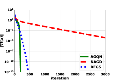
Figure 1: The convergence rates of NAGD, BFGS and the AGQN with respect to iteration number.

6.2 Verify the performance of the DAGQN

In this subsection, we test the DAGQN on the phishing and the ijcnn1 datasets from LIBSVM repertory (Chang and Lin, 2011), and compare with the distributed NAGD of first-order methods, and two second-order methods: DANE (Shamir et al., 2014) and GIANT (Wang et al., 2018). Since both DANE and GIANT need to solve a sub-problem per iteration, we adopt the conjugate gradient method (Nocedal and Wright, 2006). Besides, GIANT requires a line search method on a finite set of stepsizes for global convergence.

Firstly, for the ijcnn1 dataset where $n=22$ and $m=141691$, we set $p=100$ workers and $\tau=2$. All the training samples are divided equally among the workers. The parameters in DANE and GIANT are tuned via the methods in their original papers and are the same as that of Section 6.1 for the DAGQN and NAGD, except that the total dataset size $m$ is replaced by $m/p$. Now, we examine their convergence behaviors with respect to the communication cost between the master and a worker, which is measured by the number of communication rounds and the transmitted vectors. Then, we test two cases that $\gamma=1$ and $\gamma=0.1$. Fig. 2 confirms that the DAGQN significantly reduces the number of communication rounds. Note that both DANE and GIANT require multiple rounds of coordinated communications per iteration while one round is sufficient for the DAGQN. A similar observation can also be found in Fig. 3 for the case of transmitted $n$-dimension vectors. Besides, the smaller value of $\gamma=0.1$ slightly degrades the performance of all these methods. But the DAGQN still works better than others.

Then, for the phishing dataset, we set $p=10$ workers and $\tau=6$. And we use Fig. 4 to illustrate how the iteration number of DAGQN is affected by the parameter $\tau$, the repeated number of gBroyd updates per iteration. As expected, the total iteration number essentially decreases as $\tau$ increases.

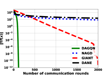
(a) ijcnn1, $\gamma=1$

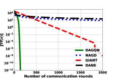
(b) ijcnn1, $\gamma=0.1$

Figure 2: $\|\nabla f\|$ versus the number of communication rounds between the master and each worker.

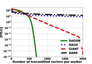
(a) ijcnn1, $\gamma=1$

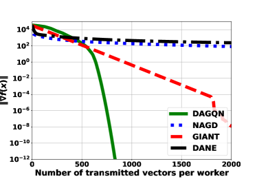
(b) ijcnn1, $\gamma=0.1$

Figure 3: $\|\nabla f\|$ versus the number of transmitted $n$-dimension vectors from each worker to the master.

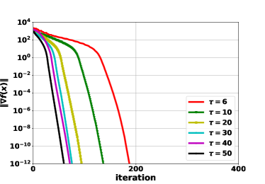
Figure 4: $\|\nabla f\|$ versus iteration number.

7 Conclusion

This paper has proposed two novel adaptive quasi-Newton methods for the both the centralized and distributed settings. They all enjoy explicit non-asymptotic bounds for both the global convergence rate and local superlinear rate, though the communication complexity of the distributed one is comparable to that of the distributed first-order methods. In the future, it is interesting to study their stochastic versions for the empirical risk problems.

Appendix A Proof of Lemma 4

Letting the right-hand side of (LABEL:equ:Broyd_inequ2) less than $\varepsilon$, we obtain a quadratic inequality in $r^{+}$, i.e.,

$$\rho(\sigma_{\tau}+n)(Mr^{+})^{2}+2\rho\sigma_{\tau}Mr^{+}+(\rho^{\tau+1}-1)\varepsilon\leq 0.$$ (61)

Since $\tau\geq 0$ and $\rho<1$, the quadratic inequality indeed has a positive solution. Specifically, if $0<Mr^{+}\leq c_{\tau,\varepsilon}$ (see (24)), then (LABEL:equ:r_inequ) holds and $\sigma_{\nabla^{2}f(x^{+})}(G^{+})\leq\varepsilon$.

By (12), $r^{+}$ can be directly controlled by $\alpha$, i.e.,

$$r^{+} =\alpha\|G^{-1}\nabla f(x)\|_{\nabla^{2}f(x)}$$ (62)

$$\leq\alpha\|G^{-1}\nabla f(x)\|_{G}=\alpha\|\nabla f(x)\|_{G}^{*}.$$

Plugging it into the above upper bound and solving the following inequality with respect to $\alpha\in(0,1]$

$$\alpha M\|\nabla f(x)\|_{G}^{*}\leq c_{\tau,\varepsilon},$$ (63)

we can easily obtain (23).

Additionally, we give a concise lower bound for $c_{\tau,\varepsilon}$ to exploit its dependence on key constants such as $n$, $\tau$ and $\kappa$. Using (24) and the ralation $\sqrt{1+a}\geq 1+\min\{a/3,\sqrt{a/3}\}$ for any $a\geq 0$, we have that

$$c_{\tau,\varepsilon}\geq$$ (64)

$$\dfrac{\sigma_{\tau}}{\sigma_{\tau}+n}\min\left\{\dfrac{\sigma_{\tau}+n}{3\rho\sigma_{\tau}^{2}}(1-\rho^{\tau+1})\varepsilon,\sqrt{\dfrac{\sigma_{\tau}+n}{3\rho\sigma_{\tau}^{2}}(1-\rho^{\tau+1})\varepsilon}\right\}.$$

Applying the relation $(1+a)^{r}\leq 1/(1-ra),a\in[-1,1/r),r\geq 0$ to $\rho^{\tau+1}$ (recall that $\rho=1-1(n\kappa)$), we have that

$$\rho^{\tau+1}\leq\dfrac{n\kappa}{n\kappa+\tau+1}.$$ (65)

Substituting it into (LABEL:equ:inequ_c), we obtain the following lower bound expressed in $\Omega(\cdot)$

$$c_{\tau,\varepsilon}\geq\dfrac{(\tau+1)\varepsilon n\kappa}{3\rho(4(n\kappa)^{2}\varepsilon+4n(n\kappa)^{2})}\geq\Omega\left(\dfrac{(\tau+1)\varepsilon}{(n+\varepsilon)(\kappa n+\tau)}\right).$$ (66)

Appendix B Proof of Lemma 5

By Assumption 2 and Eq. (LABEL:equ:G_error_inequ), we have that

$$\mu I\preceq\nabla^{2}f(x)\preceq\omega I$$ (67)

$$\nabla^{2}f(x)\preceq G\preceq(1+\varepsilon)\nabla^{2}f(x).$$

Then we bound $\|I-\nabla^{2}f(x)G^{-1}\alpha\|$ as follows

$$\|I-\nabla^{2}f(x)G^{-1}\alpha\|$$ (68)

$$=\|(1-\alpha)I+\alpha\nabla^{2}f(x)(\nabla^{2}f(x)^{-1}-G^{-1})\|$$

$$\leq(1-\alpha)+\alpha\|\nabla^{2}f(x)\|\|\nabla^{2}f(x)^{-1}-G^{-1}\|$$

$$\leq(1-\alpha)+\alpha\|\nabla^{2}f(x)\|\|\nabla^{2}f(x)^{-1}\|\varepsilon/(1+\varepsilon)$$

$$\leq(1-\alpha)+\alpha\varepsilon\kappa/(1+\varepsilon)\leq 1-\alpha/2$$

where the second inequality is due to relation (LABEL:equ:nabla_G_bounds) and the last inequality comes from (27).

Now let $d=-G^{-1}\nabla f(x)$ and expand $\nabla f(x+\alpha d)$ as

$$\nabla f(x+\alpha d) =\nabla f(x)+(\nabla^{2}f(x)\cdot d)\alpha$$ (69)

$$\quad+\left\{\int_{0}^{\alpha}\left[\nabla^{2}f(x+td)-\nabla^{2}f(x)\right]dt\right\}d$$

$$=(I-\nabla^{2}f(x)G^{-1}\alpha)\nabla f(x)$$

$$\quad+\left\{\int_{0}^{\alpha}\left[\nabla^{2}f(x+td)-\nabla^{2}f(x)\right]dt\right\}d.$$

Taking Euclidean norms on both sides leads to that

$$\|\nabla f(x+\alpha d)\|\leq\|I-\nabla^{2}f(x)G^{-1}\alpha\|\|\nabla f(x)\|$$ (70)

$$\quad\quad+\|d\|\left\{\int_{0}^{\alpha}\|\nabla^{2}f(x+td)-\nabla^{2}f(x)\|dt\right\}$$

$$\leq(1-\alpha/2)\|\nabla f(x)\|+L\alpha^{2}\|d\|^{2}/2$$

$$\leq(1-\alpha/2)\|\nabla f(x)\|+L\alpha^{2}\|\nabla f(x)\|^{2}/(2\mu^{2}).$$

where Assumption 2(b) is used in the first inequality and the last inequality is due to Assumption 2(a) and (16).

Multiplying both sides with $L/(2\mu^{2})$ yields that

$$\beta(x^{+})\leq(1-\alpha/2)\beta(x)+\beta(x)^{2}\alpha^{2}.$$ (71)

Then, an “optimal” stepsize can be derived by minimizing the quadratic function with respect to $\alpha$ on the right-hand side, the details of which are straightforward and thus omitted.

Appendix C Proof of Theorem 7

Firstly, we restate Lemma 4.3 in Rodomanov and Nesterov (2021a), which is a handy tool to depict local evolution of $\lambda(x^{k})$ when Hessian estimate error is bounded.

Lemma 14.

Let $x\in\mathbb{R}^{n}$, and let $G\in\mathbb{R}^{n\times n}$ be a positive definite matrix, satisfying

$$\nabla^{2}f(x)\preceq G\preceq\eta\nabla^{2}f(x)$$ (72)

for some $\eta\geq 1$. Let

$$x^{+}\overset{\textrm{def}}{=}x-G^{-1}\nabla f(x),$$ (73)

and suppose that $M\lambda(x)\leq 2$. Then $r^{+}\overset{\textrm{def}}{=}\|x^{+}-x\|_{\nabla^{2}f(x)}\leq\lambda(x)$, and

$$\lambda(x^{+})\leq\left(1+\dfrac{M\lambda(x)}{2}\right)\dfrac{\eta-1+M\lambda(x)/2}{\eta}\lambda(x).$$ (74)

Condition (33) ensures that the stepsize of the AGQN becomes 1. Jointly with Lemma 4, the initial condition $\sigma_{\nabla^{2}f(x^{0})}(G^{0})\leq\varepsilon$ ensures that (72) in Lemma 14 holds with $\eta=1+\varepsilon_{0}$ for all $k$. Then, by applying Lemma 14 for any $k$, we have that

$$\lambda(x^{k+1}) \leq\left(1+\dfrac{M\lambda(x^{k})}{2}\right)\dfrac{\varepsilon_{0}+M\lambda(x^{k})/2}{1+\varepsilon_{0}}\lambda(x^{k})$$ (75)

$$\leq\left(1-\dfrac{1}{1+\varepsilon_{0}}+\dfrac{M\lambda(x^{k})}{2}+\dfrac{(M\lambda(x^{k}))^{2}}{4(1+\varepsilon_{0})}\right)\lambda(x^{k})$$

$$\leq\left(\dfrac{1}{2}+\dfrac{M\lambda(x^{k})}{2}+\dfrac{(M\lambda(x^{k}))^{2}}{4}\right)\lambda(x^{k})$$

where the last inequality comes from the fact that $\varepsilon_{0}\in(0,1]$ (see (27) in Lemma 5). Then, by condition 34 and simple induction, we have that $\lambda(x^{k})$ is monotonically decreasing,

$$M\lambda(x^{k+1})\leq M\lambda(x^{k})\leq\cdots\leq M\lambda(x^{1})\leq M\lambda(x^{0})\leq 1/4.$$ (76)

Thus, we have that

$$\lambda(x^{k+1}) \leq\left(\dfrac{1}{2}+\dfrac{M\lambda(x^{k})}{2}+\dfrac{(M\lambda(x^{k}))^{2}}{4}\right)\lambda(x^{k})$$ (77)

$$\leq\left(\dfrac{1}{2}+M\lambda(x^{k})\right)\lambda(x^{k})\leq\dfrac{3}{4}\lambda(x^{k}).$$

Now we establish the superlinear rate. For the simplicity of notation, let $\lambda_{k}\overset{\textrm{def}}{=}\lambda(x^{k})$ and $\sigma_{k}\overset{\textrm{def}}{=}\sigma_{\nabla^{2}f(x^{k})}(G^{k})$. Define the following potential function:

$$\Phi_{k}\overset{\textrm{def}}{=}\sigma_{k}+4nM\lambda_{k}.$$ (78)

By invoking Lemma 14 again and we have that

$$\lambda_{k+1} \leq\left(1+\dfrac{M\lambda_{k}}{2}\right)\dfrac{\sigma_{k}+M\lambda_{k}/2}{1+\sigma_{k}}\lambda_{k}$$ (79)

$$\leq\left(1+\dfrac{M\lambda_{k}}{2}\right)\left(\sigma_{k}+4nM\lambda_{k}\right)\lambda_{k}$$

$$\leq e^{M\lambda_{k}/2}\Phi_{k}\lambda_{k}\leq e^{2M\lambda_{k}}\Phi_{k}\lambda_{k}.$$

Further, by Lemma 4.8 in Rodomanov and Nesterov (2021a) and the fact that our AGQN conducts $\tau$ additinonal gBroyd updates per iteration, we have that

$$\sigma_{k+1} \leq\rho\left(1+Mr^{k+1}\right)^{2}\left(\rho^{\tau}\sigma_{k}+\dfrac{2nMr^{k+1}}{1+Mr^{k+1}}\right)$$ (80)

$$\leq\rho\left(1+M\lambda_{k}\right)^{2}\left(\rho^{\tau}\sigma_{k}+2nM\lambda_{k}\right)$$

$$\leq\rho e^{2M\lambda_{k}}\left(\rho^{\tau}\sigma_{k}+2nM\lambda_{k}\right)$$

$$\leq e^{2M\lambda_{k}}\rho^{\tau+1}\sigma_{k}+\dfrac{3}{4}\rho e^{2M\lambda_{k}}\cdot 4nM\lambda_{k}$$

$$\leq\max\{\rho^{\tau+1},3\rho/4\}\cdot e^{2M\lambda_{k}}(\sigma_{k}+4nM\lambda_{k})$$

$$\leq\max\{\rho^{\tau+1},3\rho/4\}\cdot e^{2M\lambda_{k}}\Phi_{k}.$$

Then we focus on the evolution of $\Phi_{k}$:

$$\Phi_{k+1}=\sigma_{k+1}+4nM\lambda_{k+1}$$ (81)

$$\leq\max\{\rho^{\tau+1},3\rho/4\}\cdot e^{2M\lambda_{k}}\Phi_{k}+4nMe^{2M\lambda_{k}}\Phi_{k}\lambda_{k}$$

$$\leq\max\{\rho^{\tau+1},3\rho/4\}\cdot e^{2M\lambda_{k}}\Phi_{k}\left(1+\dfrac{4nM\lambda_{k}}{\max\{\rho^{\tau+1},3\rho/4\}}\right).$$

To avoid the trivial case, we assume that $n\geq 2$, then we have that

$$\max\{\rho^{\tau+1},3\rho/4\}\geq 3\rho/4 =3/4\times(1-1/(n\kappa))$$ (82)

$$\geq 3/4\times 1/2=3/8.$$

Subsequently,

$$\Phi_{k+1} \leq\max\{\rho^{\tau+1},3\rho/4\}\cdot e^{2M\lambda_{k}}\Phi_{k}\left(1+12nM\lambda_{k}\right)$$ (83)

$$\leq\max\{\rho^{\tau+1},3\rho/4\}\cdot\Phi_{k}e^{2M(6n+1)\lambda_{k}}$$

$$\leq\left(\max\{\rho^{\tau+1},3\rho/4\}\right)^{k+1}\cdot\Phi_{0}e^{2M(6n+1)\sum_{i=0}^{k}\lambda_{i}}.$$

Using the local linear rate of $\lambda_{k}$ in the above, we have that

$$e^{2M(6n+1)\sum_{i=0}^{k}\lambda_{i}} \leq e^{2(6n+1)M\lambda_{0}\sum_{i=0}^{k}(3/4)^{i}}$$ (84)

$$\leq e^{8(6n+1)M\lambda_{0}}\leq 2$$

where the last inequality uses condition (36). Thus we establish the linear convergence of the potential $\Phi_{k}$:

$$\Phi_{k+1}\leq\left(\max\{\rho^{\tau+1},3\rho/4\}\right)^{k+1}\cdot 2\Phi_{0}$$ (85)

where

$$\Phi_{0}=\sigma_{0}+4nM\lambda_{0}\leq\varepsilon_{0}+n\text{ln}2/(12n+2)=\bar{\Phi}_{0}.$$ (86)

Finally, we establish the superlinear convergence of $\lambda_{k}$:

$$\lambda_{k+1}\leq e^{2M\lambda_{k}}\Phi_{k}\lambda_{k}\leq e^{2M(6n+1)\lambda_{k}}\Phi_{k}\lambda_{k}$$ (87)

$$\leq e^{2M(6n+1)\lambda_{k}}\left(\max\{\rho^{\tau+1},3\rho/4\}\right)^{k}$$

$$\quad\cdot\Phi_{0}e^{2M(6n+1)\sum_{i=0}^{k-1}\lambda_{i}}\lambda_{k}$$

$$\leq\left(\max\{\rho^{\tau+1},3\rho/4\}\right)^{k}\cdot\Phi_{0}e^{2M(6n+1)\sum_{i=0}^{k}\lambda_{i}}\lambda_{k}$$

$$\leq\left(\max\{\rho^{\tau+1},3\rho/4\}\right)^{k}\cdot 2\Phi_{0}\lambda_{k}$$

$$\leq\left(\max\{\rho^{\tau+1},3\rho/4\}\right)^{k}\cdot 2\bar{\Phi}_{0}\lambda_{k}.$$

Appendix D Proof of Corollary 8

Starting from any $x^{0}\in\mathbb{R}^{n}$, we first consider the complexity of global stage, i.e., the number of iterations required before reaching the superlinear rate in Theorem 7. By Lemma 5, we have that

$$\beta(x^{k+1})\leq\begin{cases}\beta(x^{k})-1/16,\quad\quad\text{if}~{}\beta(x^{k})>1/(4\bar{\alpha}_{\tau}(x^{k})),\\ \ (1-\bar{\alpha}_{\tau}(x^{k})/4)\beta(x^{k}),\quad\text{otherwise}.\end{cases}$$ (88)

Telescoping the second case,

$$\beta(x^{k+1})\leq(1-\min\{\alpha_{\tau}(x^{k}),1\}/4)\beta(x^{k})$$ (89)

$$\leq\max\{(3/4)\beta(x^{k}),(1-\alpha_{\tau}(x^{k})/4)\beta(x^{k})\}$$

$$=\max\{(3/4)\beta(x^{k}),(1-c_{\tau,\varepsilon_{0}}/(4M\|\nabla f(x^{k})\|_{G^{k}}^{*}))\beta(x^{k})\}$$

$$\leq\max\{(3/4)\beta(x^{k}),(1-\sqrt{\mu}c_{\tau,\varepsilon_{0}}/(4M\|\nabla f(x^{k})\|))\beta(x^{k})\}$$

$$=\max\{(3/4)\beta(x^{k}),\beta(x^{k})-\sqrt{\mu}Lc_{\tau,\varepsilon_{0}}/(8M\mu^{2})\}$$

where the second inequality uses the fact that $G^{k}\succeq\nabla^{2}f(x^{k})\succeq\mu I$. Combining it with the first case, we have that

$$\beta(x^{k+1})\leq$$ (90)

$$\quad\max\left\{\frac{3}{4}\beta(x^{k}),\beta(x^{k})-\frac{\sqrt{\mu}Lc_{\tau,\varepsilon_{0}}}{8M\mu^{2}},\beta(x^{k})-\frac{1}{16}\right\}.$$

Equivalently,

$$\|\nabla f(x^{k+1})\|$$ (91)

$$\leq\max\left\{\frac{3}{4}\|\nabla f(x^{k})\|,\|\nabla f(x^{k})\|-\min\left\{\frac{\sqrt{\mu}c_{\tau,\varepsilon_{0}}}{4M},\frac{\mu^{2}}{8L}\right\}\right\}$$

$$\leq\max\left\{\frac{3}{4}\|\nabla f(x^{k})\|,\|\nabla f(x^{k})\|-\frac{\mu^{2}}{4L}\min\{c_{\tau,\varepsilon_{0}},1/2\}\right\}$$

where we use the relation $M\leq L/\mu^{3/2}$. Then the complexity to reach condition (33) is bounded by

$$\mathcal{O}\left(\max\left\{\log\left(\frac{M\|\nabla f(x^{0})\|}{\sqrt{\mu}c_{\tau,\varepsilon_{0}}}\right),\log\left(\frac{2L\|\nabla f(x^{0})\|}{\mu^{2}}\right)\right\}\right.$$ (92)

$$\quad\quad\left.+\frac{4L\|\nabla f(x^{0})\|}{\mu^{2}\min\{c_{\tau,\varepsilon_{0}},1/2\}}\right).$$

Using $M\leq L/\mu^{3/2}$, (66) and (27) and hiding the $\log$ term, it becomes that

$$\widetilde{\mathcal{O}}\left(\frac{nL(\kappa n+\tau)\kappa}{\mu^{2}\tau}\|\nabla f(x^{0})\|\right).$$ (93)

For condition 36, considering that $\lambda(x)\leq\|\nabla f(x)\|/\sqrt{\mu}$, its complexity can be similarly bounded by (93) and we omit it.

For the superlinear stage, using (65), we have that

$$\max\{\rho^{\tau+1},3\rho/4\} \leq\rho\max\{n\kappa/(n\kappa+\tau),3/4\}$$ (94)

$$\leq 1-\max\{n\kappa/(n\kappa+\tau),3/4\}/n\kappa$$

$$=1-\max\{1/(n\kappa+\tau),3/(4n\kappa)\}.$$

Then we can simply convert the local superlinear rate in (37) to the second part of complexity in Corollary 8 by the same way as in Safaryan et al. (2022).

Appendix E Proof of Lemma 9

The proof part (a) and (b) are trivial and we omit them. By Lemma 3, for any $x,y,z,w\in\mathbb{R}^{n}$, we have that

$$\nabla^{2}f(x)-\nabla^{2}f(y)=\sum_{i=1}^{p}(\nabla^{2}f_{i}(x)-\nabla^{2}f_{i}(y))$$ (95)

$$\leq M\sum_{i=1}^{p}\|x-y\|_{\nabla^{2}f_{i}(z)}\nabla^{2}f_{i}(w)$$

$$\leq M\nabla^{2}f(w)\sum_{i=1}^{p}\|x-y\|_{\nabla^{2}f_{i}(z)}$$

$$\leq M\nabla^{2}f(w)p\left((1/p)\sum_{i=1}^{p}\|x-y\|^{2}_{\nabla^{2}f_{i}(z)}\right)^{1/2}$$

$$=\sqrt{p}M\nabla^{2}f(w)\|x-y\|_{\nabla^{2}f(z)}$$

where the second inequality uses $\nabla^{2}f_{i}(w)\succ 0$, the third inequality comes from the power mean inequality $(1/p)\sum_{i=1}^{p}a_{i}\leq((1/p)\sum_{i=1}^{p}a_{i}^{2})^{1/2}$ for any $a_{i}\geq 0$. The proof is finished.

Appendix F Proof of Lemma 11

Similar with the proof of Lemma 4 (see Appendix A), using Lemma 10 and 16, we actually want the following to hold:

$$\rho(1+Mr^{+})^{2}\left(\rho^{\tau}\varepsilon+\dfrac{2n\sqrt{p}Mr^{+}}{1+Mr^{+}}\right)\leq\varepsilon.$$ (96)

Rearrange it and we obtain the following inequality in $r^{+}$,

$$\rho(\sigma_{\tau}+n\sqrt{p})(Mr^{+})^{2}+2\rho\sigma_{\tau}Mr^{+}+(\rho^{\tau+1}-1)\varepsilon\leq 0$$ (97)

where $\sigma_{\tau}=\rho^{\tau}\varepsilon+n\sqrt{p}$. It is straightforward to verify that if $Mr^{+}\leq c_{\tau,\varepsilon}$ (see (47)), (LABEL:equ:r_inequ_Delta) holds and thus $\Delta_{\nabla^{2}f(x^{+})}(G^{+})\leq\varepsilon$.

Then by $G=\sum_{i=1}^{p}G^{i}\succeq\sum_{i=1}^{p}\nabla^{2}f_{i}(x)=\nabla^{2}f(x)$, we have that

$$r^{+} =\alpha\|G^{-1}\nabla f(x)\|_{\nabla^{2}f(x)}$$ (98)

$$\leq\alpha\|G^{-1}\nabla f(x)\|_{G}=\alpha\|\nabla f(x)\|_{G}^{*}.$$

Plugging it into $Mr^{+}\leq c_{\tau,\varepsilon}$, we have that

$$\alpha M\|\nabla f(x)\|_{G}^{*}\leq c_{\tau,\varepsilon}.$$ (99)

Solve it with respect to $\alpha$ and obtain (46).

Appendix G Proof of Theorem 12

Firstly we give a lemma to show that $\Delta_{\nabla^{2}f(x)}(G)$ is an upper bound of $\sigma_{\nabla^{2}f(x)}(G)$.

Lemma 15.

Suppose that $G=\sum_{i=1}^{p}G_{i}$ and $G_{i}\succeq\nabla^{2}f_{i}(x)\succ 0$ for each $i\in\mathcal{P}$. It holds that

$$\sigma_{\nabla^{2}f(x)}(G)\leq\Delta_{\nabla^{2}f(x)}(G).$$ (100)

By the definition of $\sigma_{A}(G)$ in (9), we have that

$$\sigma_{\nabla^{2}f(x)}(G) =\langle\nabla^{2}f(x)^{-1},G-\nabla^{2}f(x)\rangle$$ (101)

$$=\sum_{i=1}^{p}\langle\nabla^{2}f(x)^{-1},G_{i}-\nabla^{2}f_{i}(x)\rangle$$

$$\leq\sum_{i=1}^{p}\langle\nabla^{2}f_{i}(x)^{-1},G_{i}-\nabla^{2}f_{i}(x)\rangle$$

$$=\sum_{i=1}^{p}\sigma_{\nabla^{2}f_{i}(x)}(G_{i})=\Delta_{\nabla^{2}f(x)}(G)$$

where the inequality comes from the fact that $\nabla^{2}f(x)=\sum_{i=1}^{p}\nabla^{2}f_{i}(x)\succ\nabla^{2}f_{i}(x)$ since $\nabla^{2}f_{i}(x)\succ 0$ for all $i$.

The following lemma quantifies how $\Delta_{\nabla^{2}f(x)}(G)$ evolves as $x$ is updated to $x^{+}$.

Lemma 16.

Let $x\in\mathbb{R}^{n}$, and let $G\overset{\textrm{def}}{=}\sum_{i=1}^{p}G_{i}$ where $G_{i}\in\mathbb{R}^{n\times n}$ is a positive definite matrix satisfying $\nabla^{2}f_{i}(x)\preceq G_{i}$ for all $i\in\mathcal{P}$. Let $x^{+}\in\mathbb{R}^{n}$, $r_{i}^{+}\overset{\textrm{def}}{=}\|x^{+}-x\|_{\nabla^{2}f_{i}(x)}$ and $G^{+}\overset{\textrm{def}}{=}\sum_{i=1}^{p}G_{i}^{+}$ where

$$G_{i}^{+}=\textrm{gBroyd}(\overline{G}^{+},\nabla^{2}f_{i}(x^{+})),~{}~{}~{}\overline{G}_{i}^{+}=(1+Mr_{i}^{+})G_{i}.$$ (102)

Then we have that

$$\Delta_{\nabla^{2}f(x^{+})}(G^{+})$$ (103)

$$\quad\quad\leq\rho(1+Mr^{+})^{2}\left(\Delta_{\nabla^{2}f(x)}(G)+\dfrac{2n\sqrt{p}Mr^{+}}{1+Mr^{+}}\right)$$

where $r^{+}\overset{\textrm{def}}{=}\|x^{+}-x\|_{\nabla^{2}f(x)}$ and $\rho\overset{\textrm{def}}{=}1-1/(n\kappa)$.

Applying Lemma 4.8 to each $G_{i}$, we have that

$$\sigma_{\nabla^{2}f_{i}(x^{+})}(G_{i}^{+})$$ (104)

$$\quad\quad\leq\rho(1+Mr_{i}^{+})^{2}\left(\sigma_{\nabla^{2}f_{i}(x)}(G_{i})+\dfrac{2nMr_{i}^{+}}{1+Mr_{i}^{+}}\right).$$

Taking sum over $i$, we have that

$$\Delta_{\nabla^{2}f(x^{+})}(G^{+})$$ (105)

$$\leq\rho\sum_{i=1}^{p}(1+Mr_{i}^{+})\left(\sigma_{\nabla^{2}f_{i}(x)}(G_{i})(1+Mr_{i}^{+})+2nMr_{i}^{+}\right)$$

$$\leq\rho(1+Mr^{+})\left(\sum_{i=1}^{p}\sigma_{\nabla^{2}f_{i}(x)}(G_{i})(1+Mr_{i}^{+})\right.$$

$$\quad\left.+2nM\sum_{i=1}^{p}r_{i}^{+}\right)$$

$$\leq\rho(1+Mr^{+})\left((1+Mr^{+})\Delta_{\nabla^{2}f(x)}(G)+2n\sqrt{p}Mr^{+}\right)$$

$$=\rho(1+Mr^{+})^{2}\left(\Delta_{\nabla^{2}f(x)}(G)+\dfrac{2n\sqrt{p}Mr^{+}}{1+Mr^{+}}\right),$$

which the second and third equalities come from the relation $r^{+}=(\sum_{i=1}^{p}(r_{i}^{+})^{2})^{1/2}\geq r_{i}^{+}$ and the power mean equality $(1/p)\sum_{i=1}^{p}a_{i}\leq((1/p)\sum_{i=1}^{p}a_{i}^{2})^{1/2}$.

G.1 Proof of part (a)

With the initial conditions in Theorem 12, applying Lemma 11 and Lemma 15, we have that

$$\nabla^{2}f(x^{k})\preceq G^{k} \preceq(1+\sigma_{x}(G^{k}))\nabla^{2}f(x^{k})$$ (106)

$$\preceq(1+\Delta_{x}(G^{k}))\nabla^{2}f(x^{k})$$

$$\preceq(1+\epsilon_{0})\nabla^{2}f(x^{k}),~{}~{}~{}\forall k.$$

Note that $f$ has the same condition number $\kappa$ as each $f_{i}$. The remaining proof is the same as that of Lemma 5 (see the Appendix B) except that $\alpha_{\tau}(x)$ now is given by Lemma 11 and $\beta(x)$ for $f$ in (39) is defined in (49).

G.2 Proof of part (b)

With the initial condition given in (52) and the global convergence guarantee, it is straightforward to verify that $\alpha(x^{k})=1$ for all $k\geq 0$. Given (106) and the initial condition (53), we can apply Lemma 14 for any $k$, and have that

$$\lambda(x^{k+1}) \leq\left(1+\dfrac{M_{f}\lambda(x^{k})}{2}\right)\dfrac{\varepsilon_{0}+M_{f}\lambda(x^{k})/2}{1+\varepsilon_{0}}\lambda(x^{k}).$$ (107)

The remaining proof is the same as that of Theorem 7 (see Appendix C) and we omit it.

G.3 Proof of part (c)

For the simplicity of notation, let $\lambda_{k}\overset{\textrm{def}}{=}\lambda(x^{k})$ and $\Delta_{k}\overset{\textrm{def}}{=}\Delta_{\nabla^{2}f(x^{k})}(G^{k})$. Define the following potential function:

$$\Phi_{k}\overset{\textrm{def}}{=}\sigma_{k}+4n\sqrt{p}M\lambda_{k}.$$ (108)

Since all the conditions of part (b) are also satisfied in part(c), we can invoke Lemma 14 again and have that

$$\lambda_{k+1} \leq\left(1+\dfrac{M_{f}\lambda_{k}}{2}\right)\dfrac{\Delta_{k}+M_{f}\lambda_{k}/2}{1+\Delta_{k}}\lambda_{k}$$ (109)

$$\leq\left(1+\dfrac{M_{f}\lambda_{k}}{2}\right)\left(\Delta_{k}+4n\sqrt{p}M\lambda_{k}\right)\lambda_{k}$$

$$\leq e^{M_{f}\lambda_{k}/2}\Phi_{k}\lambda_{k}\leq e^{2\sqrt{p}M\lambda_{k}}\Phi_{k}\lambda_{k}$$

where the second and last inequality use the relation $M_{f}\leq\sqrt{p}M$ in Lemma 9.

Further, by Lemma 10 and 16, we have that

$$\Delta_{k+1} \leq\rho\left(1+Mr^{k+1}\right)^{2}\left(\rho^{\tau}\Delta_{k}+\dfrac{2n\sqrt{p}Mr^{k+1}}{1+Mr^{k+1}}\right)$$ (110)

$$\leq\rho\left(1+M\lambda_{k}\right)^{2}\left(\rho^{\tau}\Delta_{k}+2n\sqrt{p}M\lambda_{k}\right)$$

$$\leq\rho e^{2M\lambda_{k}}\left(\rho^{\tau}\Delta_{k}+2n\sqrt{p}M\lambda_{k}\right)$$

$$\leq e^{2M\lambda_{k}}\rho^{\tau+1}\Delta_{k}+\dfrac{3}{4}\rho e^{2M\lambda_{k}}\cdot 4n\sqrt{p}M\lambda_{k}$$

$$\leq\max\{\rho^{\tau+1},3\rho/4\}\cdot e^{2M\lambda_{k}}(\Delta_{k}+4n\sqrt{p}M\lambda_{k})$$

$$\leq\max\{\rho^{\tau+1},3\rho/4\}\cdot e^{2M\lambda_{k}}\Phi_{k}.$$

Then we focus on the evolution of $\Phi_{k}$:

$$\Phi_{k+1}=\Delta_{k+1}+4n\sqrt{p}M\lambda_{k+1}$$ (111)

$$\leq\max\{\rho^{\tau+1},3\rho/4\}\cdot e^{2M\lambda_{k}}\Phi_{k}+4n\sqrt{p}Me^{2\sqrt{p}M\lambda_{k}}\Phi_{k}\lambda_{k}$$

$$\leq\max\{\rho^{\tau+1},3\rho/4\}\cdot\Phi_{k}\left(1+\dfrac{4n\sqrt{p}M\lambda_{k}}{\max\{\rho^{\tau+1},3\rho/4\}}\right)\cdot$$

$$\quad e^{2\sqrt{p}M\lambda_{k}}.$$

By (82), we have that

$$\max\{\rho^{\tau+1},3\rho/4\}\geq=3/8.$$ (112)

Then,

$$\Phi_{k+1} \leq\max\{\rho^{\tau+1},3\rho/4\}\cdot e^{2\sqrt{p}M\lambda_{k}}\Phi_{k}\left(1+12n\sqrt{p}M\lambda_{k}\right)$$ (113)

$$\leq\max\{\rho^{\tau+1},3\rho/4\}\cdot\Phi_{k}e^{2\sqrt{p}M(6n+1)\lambda_{k}}$$

$$\leq\left(\max\{\rho^{\tau+1},3\rho/4\}\right)^{k+1}\cdot\Phi_{0}e^{2\sqrt{p}M(6n+1)\sum_{i=0}^{k}\lambda_{i}}.$$

Using the local linear rate of $\lambda_{k}$ in part (b), we have that

$$e^{2\sqrt{p}M(6n+1)\sum_{i=0}^{k}\lambda_{i}} \leq e^{2(6n+1)\sqrt{p}M\lambda_{0}\sum_{i=0}^{k}(3/4)^{i}}$$ (114)

$$\leq e^{8(6n+1)\sqrt{p}M\lambda_{0}}\leq 2$$

where the last inequality uses condition (55). Thus we establish the linear convergence of the potential $\Phi_{k}$:

$$\Phi_{k+1}\leq\left(\max\{\rho^{\tau+1},3\rho/4\}\right)^{k+1}\cdot 2\Phi_{0}$$ (115)

where

$$\Phi_{0}=\Delta_{0}+4n\sqrt{p}M\lambda_{0}\leq\varepsilon_{0}+n\text{ln}2/(12n+2)=\bar{\Phi}_{0}.$$ (116)

Finally, we establish the superlinear convergence of $\lambda_{k}$:

$$\lambda_{k+1}\leq e^{2\sqrt{p}M\lambda_{k}}\Phi_{k}\lambda_{k}\leq e^{2\sqrt{p}M(6n+1)\lambda_{k}}\Phi_{k}\lambda_{k}$$ (117)

$$\leq e^{2\sqrt{p}M(6n+1)\lambda_{k}}\left(\max\{\rho^{\tau+1},3\rho/4\}\right)^{k}\cdot\lambda_{k}$$

$$\quad\cdot\Phi_{0}e^{2\sqrt{p}M(6n+1)\sum_{i=0}^{k-1}\lambda_{i}}$$

$$\leq\left(\max\{\rho^{\tau+1},3\rho/4\}\right)^{k}\cdot\lambda_{k}\Phi_{0}e^{2\sqrt{p}M(6n+1)\sum_{i=0}^{k}\lambda_{i}}$$

$$\leq\left(\max\{\rho^{\tau+1},3\rho/4\}\right)^{k}\cdot 2\Phi_{0}\lambda_{k}$$

$$\leq\left(\max\{\rho^{\tau+1},3\rho/4\}\right)^{k}\cdot 2\bar{\Phi}_{0}\lambda_{k}$$

where the fifth inequality follows from (114). The proof is finished.

References

• (1)
• Agafonov et al. (2022) Agafonov, A., Kamzolov, D., Tappenden, R., Gasnikov, A. and Takáč, M. (2022), ‘Flecs: A federated learning second-order framework via compression and sketching’, arXiv preprint arXiv:2206.02009 .
• Alimisis et al. (2021) Alimisis, F., Davies, P. and Alistarh, D. (2021), Communication-efficient distributed optimization with quantized preconditioners, in ‘International Conference on Machine Learning’, pp. 196–206.
• Boyd and Vandenberghe (2004) Boyd, S. and Vandenberghe, L. (2004), Convex Optimization, Cambridge University Press.
• Chang and Lin (2011) Chang, C.-C. and Lin, C.-J. (2011), ‘Libsvm: a library for support vector machines’, ACM Transactions on Intelligent Systems and Technology 2(3), 1–27.
• Crane and Roosta (2019) Crane, R. and Roosta, F. (2019), Dingo: Distributed newton-type method for gradient-norm optimization, in ‘Advances in Neural Information Processing Systems 32’, pp. 9498–9508.
• Crane and Roosta (2020) Crane, R. and Roosta, F. (2020), DINO: distributed newton-type optimization method, in ‘International Conference on Machine Learning’, pp. 2174–2184.
• Du and You (2021) Du, Y. and You, K. (2021), ‘Asynchronous stochastic gradient descent over decentralized datasets’, IEEE Transactions on Control of Network Systems 8(3), 1212–1224.
• Du and You (2022) Du, Y. and You, K. (2022), Greedy quasi-newton methods with explicit superlinear convergence, in ‘61st IEEE Conference on Decision and Control, Cancun, Mexico, USA’.
• Eisen et al. (2017) Eisen, M., Mokhtari, A. and Ribeiro, A. (2017), ‘Decentralized quasi-newton methods’, IEEE Transactions on Signal Processing 65(10), 2613–2628.
• Fabbro et al. (2022) Fabbro, N. D., Dey, S., Rossi, M. and Schenato, L. (2022), ‘A newton-type algorithm for federated learning based on incremental hessian eigenvector sharing’, arXiv preprint arXiv:2202.05800 .
• Horn and Johnson (2012) Horn, R. A. and Johnson, C. R. (2012), Matrix Analysis, Cambridge University Press.
• Islamov et al. (2021) Islamov, R., Qian, X. and Richtarik, P. (2021), Distributed second order methods with fast rates and compressed communication, in ‘International Conference on Machine Learning’, pp. 4617–4628.
• Jin and Mokhtari (2022) Jin, Q. and Mokhtari, A. (2022), ‘Non-asymptotic superlinear convergence of standard quasi-Newton methods’, Mathematical Programming pp. 1–49.
• Leblond et al. (2017) Leblond, R., Pedregosa, F. and Lacoste-Julien, S. (2017), Asaga: asynchronous parallel saga, in ‘Artificial Intelligence and Statistics’, pp. 46–54.
• Lee et al. (2018) Lee, C.-p., Lim, C. H. and Wright, S. J. (2018), A distributed quasi-newton algorithm for empirical risk minimization with nonsmooth regularization, in ‘ACM SIGKDD International Conference on Knowledge Discovery and Data Mining’, pp. 1646–1655.
• Li et al. (2021) Li, Y., Gong, Y., Freris, N. M., Voulgaris, P. and Stipanović, D. (2021), BFGS-ADMM for large-scale distributed optimization, in ‘60th IEEE Conference on Decision and Control’, pp. 1689–1694.
• Li et al. (2022) Li, Y., Voulgaris, P. G. and Freris, N. M. (2022), A communication efficient quasi-Newton method for large-scale distributed multi-agent optimization, in ‘IEEE International Conference on Acoustics, Speech and Signal Processing’, pp. 4268–4272.
• Lian et al. (2015) Lian, X., Huang, Y., Li, Y. and Liu, J. (2015), Asynchronous parallel stochastic gradient for nonconvex optimization, in ‘Advances in Neural Information Processing Systems 28’, pp. 2737–2745.
• Liu et al. (2015) Liu, J., Wright, S. J., Re, C., Bittorf, V. and Sridhar, S. (2015), ‘An asynchronous parallel stochastic coordinate descent algorithm’, Journal of Machine Learning Research 16(1), 285–322.
• Malitsky and Mishchenko (2020) Malitsky, Y. and Mishchenko, K. (2020), Adaptive gradient descent without descent, in ‘International Conference on Machine Learning’, pp. 6702–6712.
• Mansoori and Wei (2020) Mansoori, F. and Wei, E. (2020), ‘A fast distributed asynchronous newton-based optimization algorithm’, IEEE Transactions on Automatic Control 65(7), 2769–2784.
• Mishchenko (2021) Mishchenko, K. (2021), ‘Regularized newton method with global $o(1/k^{2})$ convergence’, arXiv preprint arXiv:2112.02089 .
• Mokhtari et al. (2016) Mokhtari, A., Ling, Q. and Ribeiro, A. (2016), ‘Network newton distributed optimization methods’, IEEE Transactions on Signal Processing 65(1), 146–161.
• Nesterov (2003) Nesterov, Y. (2003), Introductory lectures on convex optimization: A basic course, Vol. 87, Springer Science & Business Media.
• Nocedal and Wright (2006) Nocedal, J. and Wright, S. (2006), Numerical optimization, Springer Science & Business Media.
• Pearlmutter (1994) Pearlmutter, B. A. (1994), ‘Fast exact multiplication by the hessian’, Neural computation 6(1), 147–160.
• Polyak and Tremba (2020) Polyak, B. and Tremba, A. (2020), ‘New versions of newton method: step-size choice, convergence domain and under-determined equations’, Optimization Methods and Software 35(6), 1272–1303.
• Recht et al. (2011) Recht, B., Re, C., Wright, S. and Niu, F. (2011), Hogwild: A lock-free approach to parallelizing stochastic gradient descent, in ‘Advances in Neural Information Processing Systems 24’, pp. 693–701.