Abstract

High-dimensional time series data poses challenges due to its dynamic nature, varying lengths, and presence of missing values. This kind of data requires extensive preprocessing, limiting the applicability of existing Time Series Classification and Time Series Extrinsic Regression techniques. For this reason, we propose BORF, a Bag-Of-Receptive-Fields model, which incorporates notions from time series convolution and 1D-SAX to handle univariate and multivariate time series with varying lengths and missing values. We evaluate BORF on Time Series Classification and Time Series Extrinsic Regression tasks using the full UEA and UCR repositories, demonstrating its competitive performance against state-of-the-art methods. Finally, we outline how this representation can naturally provide saliency and feature-based explanations.

1 Introduction

High-dimensional time series data is becoming more widely available to decision-makers, domain experts, and researchers. This kind of data, by definition, captures dynamic changes over time and is used in many fields, including finance, healthcare, and environmental science (Shumway et al.,, 2000). Sensors often record such data at different frequencies or for varying lengths of time, resulting in signals with a different number of observations. Sensors can also fail, leaving gaps and missing values in time series signals. Because of these factors, real-world time series data is frequently “dirty” and difficult to handle, necessitating extensive preprocessing (Kreindler and Lumsden,, 2006). These complexities present significant challenges to most existing time series analysis techniques, frequently developed and tested on very clean datasets, limiting their applicability in real-world scenarios (Bagnall et al.,, 2017; Ruiz et al.,, 2021).

Within time series analysis (TSA), Time Series Classification (TSC), and Time Series Extrinsic Regression (TSER) are extremely relevant tasks. TSC is the task of predicting a categorical value from a time series, for example, distinguishing between a healthy and unhealthy patient given vital signals (Bagnall et al.,, 2017). TSER is instead the task of predicting a scalar, i.e., a continuous value (Tan et al.,, 2021). TSER differs from time series forecasting (TSF), also called time series regression (TSR). The term “extrinsic” emphasizes that, in TSER, contrary to TSF (or TSR), the predicted value may not be the future of the analyzed series (Tan et al.,, 2021). Research into TSER has received much less attention in the time series research community, even if it models interesting problems (Tan et al.,, 2020), such as predicting energy consumption by monitoring rooms in houses (Hebrail and Berard,, 2012). Further, TSER and TSC approaches should be as interpretable as possible to ensure applicability in critical domains. In contrast, state-of-the-art models for TSA are mainly black-box models (Theissler et al.,, 2022). Additionally, when the number of observations in a time series dataset is irregular or there are missing values, these models require several preprocessing steps.

Given these challenges, we propose borf, a Bag-Of-Receptive-Fields. borf is a deterministic time series transform that converts any time series dataset into an easier-to-handle, understandable tabular representation. borf is very flexible in the input type, allowing the processing of real-world multivariate time series with irregular signals of different lengths and containing missing values. This is achieved by processing signals independently and generalizing pattern discretization through complete case analysis. Further, to ensure an expressive representation, we introduce convolutional operators to extract receptive fields from the time series. Unlike standard subsequences, receptive fields can better describe the development of a time series at different resolutions and highlight its local and global characteristics. We show that the novel connection between convolutional operators and multi-resolution symbolic patterns allows for great performance in TSC and TSER. We test borf on the full UEA and UCR repositories, comprising $177$ datasets, against several state-of-the-art approaches, $12$ for TSC and $6$ for TSER. We show that borf challenges competitor models in TSC and outperforms them in TSER. Finally, we propose a scalable heuristic in time and space complexity and define a connection between feature and saliency-based explanations in a borf representation, outlining its natural interpretability.

The rest of the paper is organized as follows. Sec. 2 discusses the related work and main competitors, while Sec. 3 summarizes the background of our proposal. borf is presented in Sec. 4, and tested in Sec. 5. Finally, we present our conclusions in Sec. 6.

2 Related Work

The field of time series predictors encompasses a wide range of approaches (Ruiz et al.,, 2021; Tan et al.,, 2021). Our proposal belongs to the dictionary-based category, which extracts features from time series by recording characteristics of discretized subpatterns (Bagnall et al.,, 2017). These methods segment time series into subsequences, convert them into symbolic words, and create histograms of feature counts (Baydogan et al.,, 2013). For this reason, they rely heavily on effective time series approximation methods such as the Symbolic Aggregate approXimation (SAX) (Lin et al.,, 2007) and Symbolic Fourier Approximation (SFA) (Schäfer and Högqvist,, 2012). SAX uses Piecewise Aggregate Approximation (PAA) (Keogh et al.,, 2001) for segmentation and binning, while SFA focuses on spectral properties using Fourier coefficients (Schäfer and Högqvist,, 2012). Although informative for certain applications, SFA loses temporal information and has higher computational complexity than SAX (Schäfer and Högqvist,, 2012). Notably, 1D-SAX was introduced to enhance SAX representation by using Piecewise Linear Approximation (PLA) (Hung and Anh,, 2007) instead of PAA, to infer segment slopes (Malinowski et al.,, 2013), but it has yet to be adopted in dictionary-based approaches.

In general, even if subsequence extraction can be implemented in supervised and unsupervised ways, it is mainly applied to TSC. The first dictionary-based method is the traditional Bag-of-Patterns (bop) (Lin et al.,, 2012), which uses SAX to generate discretized subsequences, counting their frequency. Other methods rely on supervised techniques by introducing a tf-idf weighing of features (sax-vsm) (Senin and Malinchik,, 2013), or by filtering subsequences extracted with SAX and SFA through a Chi-squared bound (mr-sqm) (Nguyen and Ifrim,, 2022). boss (Bag-of-SFA-Symbols) (Schäfer,, 2015) and its more recent extension, weasel+muse (Schäfer and Leser,, 2017), focus on the sole usage of SFA and achieve state-of-the-art performance in multivariate time series classification. Being specifically developed for TSC, the main limitation of these classifiers is that they cannot be easily extended to other tasks. Specifically, to the best of our knowledge, none was ever tested on TSER. Unlike most of the previously mentioned approaches, borf is unsupervised and, to the best of our knowledge, is the first dictionary-based method capable of effectively tackling both TSC and TSER tasks. We achieve superior performance by proposing theoretical and practical extensions, introducing several generalizations addressing the primary limitations of bop. Specifically, borf allows for extracting multi-resolution 1D-SAX patterns from univariate and multivariate time series data, accommodating signals of varying lengths and those with missing values. Dictionary-based features, i.e., time series patterns, seem particularly well-suited for explaining prediction outcomes via feature importance or saliency maps. Yet, the interpretability of such approaches is rarely evaluated (Theissler et al.,, 2022). For instance, in (Spinnato et al.,, 2022), SAX words are employed to explain tree-based models, but the explanation is limited to feature importance and lacks mapping to time series as saliency maps. Le Nguyen et al., (2019) demonstrate how coefficients assigned to SAX words in a linear model can be mapped back to the original time series. However, this explanation is class-wise and insufficient for interpreting the prediction outcomes of individual time series instances. We emphasize how borf naturally enables local explanations based on saliency maps and feature importance.

The most famous pattern-based TSC approaches are based on shapelets. These methods focus on finding short patterns that define a class independently of the position of the pattern (Ye and Keogh,, 2011). The discriminative feature is usually a distance, which can be used to convert the time series dataset into a tabular one through the so-called shapelet transform (Lines et al.,, 2012). Many approaches in this field use different ways of extracting shapelets and building the subsequent classifier. For example, in the Random Shapelet Forest (rsf) algorithm (Karlsson et al.,, 2016), the shapelets are sampled randomly, building a forest of decision trees with these shapelets as splitting points. According to (Bagnall et al.,, 2017), the Shapelet Transform (st) (Hills et al.,, 2014) algorithm is still the most accurate shapelet approach, with the drawback of the high computational complexity resulting in rather long training and inference times. To the best of our knowledge, rsf is the only shapelet-based approach that can be used for TSER.

Interval-based classifiers, such as Time Series Forest (tsf) (Deng et al.,, 2013) and bag-of-features framework (tsbf) (Baydogan et al.,, 2013), divide time series into random intervals and extract summary statistics like mean, standard deviation, and slope, training a random forest on the resulting dataset. The state-of-the-art approach in this category is the Canonical Interval Forest (cif) (Middlehurst et al.,, 2020), which combines tsf and Random Interval Spectral Ensemble (rise) (Flynn et al.,, 2019) methods. Notably, these approaches heavily rely on randomization, causing variations in the areas of interest used by the classifier across runs. In contrast, borf is entirely deterministic, generating repeatable representations.

Finally, rocket (Dempster et al.,, 2020) generates many random convolutional kernels to transform time series into feature vectors, which can be used with any linear classifier or regressor, often achieving high accuracy and processing speed even with large and complex datasets. rocket is currently the best-performing model in both TSC and TSER (Ruiz et al.,, 2021; Tan et al.,, 2021). Inspired by the great performance of such an approach, we also introduce convolution operators inside borf. As a final note, deep learning approaches often fall behind in this task (Ruiz et al.,, 2021), given that they require ad-hoc fine-tuning, often dependent on the specific task and dataset.

3 Background

This section provides all the necessary concepts to understand our proposal. We begin by defining time series data.

Definition 1 (Time Series Data).

A time series dataset, $\mathcal{{X}}=\{{X}_{1},\dots,{X}_{n}\}\in\dot{\mathbb{R}}^{n\times c\times m}$, is a collection of $n$ time series. A time series, ${X}$, is a collection of $c$ signals (or channels), ${X}=\{\textbf{x}_{1},\dots,\textbf{x}_{c}\}\in\dot{\mathbb{R}}^{c\times m}$. A signal, x, is a sequence of $m$ real-valued observations sampled at equal time intervals, $\textbf{x}=[x_{1},\dots,x_{m}]\in\dot{\mathbb{R}}^{m}$. Associated with each signal, is a timestep vector $\textbf{t}=[t_{1},\dots,t_{m}]=[1,\dots,m]\in\mathbb{N}^{m}$, which contains the index of the recorded observation.

When $c=1$, the time series is univariate, else it is multivariate. For simplicity of notation, we use a unique symbol $m$ to denote the lengths of the time series. However, signals in each time series can generally have different lengths. We use the overdot over a set, (e.g., $\dot{\mathbb{R}}$) to indicate the extension to NaN values, representing a symbol for a missing observation (e.g., $\mathbb{R}\cup\{\textit{NaN}\}$).

Time series datasets can be used in a variety of tasks. This work focuses on supervised learning, particularly time series extrinsic predictions.

Definition 2 (Time Series Extrinsic Prediction).

Given a time series dataset, $\mathcal{{X}}$, Time Series Extrinsic Prediction is the task of training a model, $f$, to predict an output, $y$, for each input time series, ${X}$, i.e., $f(\mathcal{{X}})=[f({X}_{1}),\dots,f({X}_{n})]=\textbf{y}$.

If the values in y are categorical, i.e., $\textbf{y}\in\mathbb{N}^{n}$, the task is called Time Series Classification (TSC). If the values are scalars, i.e., $\textbf{y}\in\mathbb{R}^{n}$, the task is called Time Series Extrinsic Regression (TSER).

Two of the most common XAI techniques for explaining extrinsic predictions are feature importance and saliency maps (Bodria et al.,, 2023).

Definition 3 (Feature Importance).

Give an instance of a tabular dataset, $\textbf{p}\in\mathbb{R}^{h}$, a feature importance vector, $\boldsymbol{\phi}=[\phi_{1},\dots,\phi_{h}]\in\mathbb{R}^{h}$, contains a score for each value in p.

Definition 4 (Saliency Map).

Given a time series, ${X}$, a saliency map, $\Psi=[\psi_{1,1},\dots,\psi_{c,m}]\in\mathbb{R}^{c,m}$, contains a score, $\psi_{k,j}$, for every observation, $x_{k,j}$, in ${X}$.

These are similar concepts that differ in the input type. Feature importance highlights the relevance of features in a tabular dataset, while saliency maps are adopted in computer vision to highlight the contribution of single observations toward time series predictions. These explanations are strongly connected in our proposal, as shown in Section 5.

4 Proposed Method

Input: $\mathcal{{X}}$ - time series dataset, $w$ - window size, $d$ - dilation, $s$ - stride, $l$ - word length, $a_{\mu}$ - mean alphabet size, $a_{\beta}$ - slope alphabet size, $\theta$ - standard deviation threshold

Output: ${P}$ - Bag-of-Receptive-Fields

1 ${P}\leftarrow\emptyset$;

2for ${X}_{i}\in\mathcal{{X}}$ do

3       for $\textbf{x}\in{X}$ do

4             ${R}\leftarrow\textit{{{windowize}}}(\textbf{x},w,d,s)$;

5             for $\textbf{r}\in{R}$ do

6                   $\textbf{r}\leftarrow\textit{{{normalize}}}(\textbf{r},\textbf{x},\theta)$;

7                   $\tilde{\textbf{r}}\leftarrow\textit{{1d-sax-na}}(\textbf{r},l,a_{\mu},a_{\beta})$;

8                  

9                  if $[*,\tilde{\textbf{r}}]\in P$ then

10                        

11                        $P[i,\tilde{\textbf{r}}]\leftarrow P[i,\tilde{\textbf{r}}]+1$;

12                  else

13                        $P[i,\tilde{\textbf{r}}]\leftarrow 1$;

return ${P}$

Algorithm 1 borf (training)

The Bag-Of-Receptive-Fields (borf) introduces a novel connection between convolutional operators and pattern extraction by generalizing the concept of subsequence to that of a receptive field.

Definition 5 (Receptive Field).

Given a signal x, a receptive field of length $w\geq 1$ and dilation $d\geq 1$, is an ordered sequence of values, $\textbf{r}=[x_{j},x_{j+d},\dots,x_{j+d(w-1)}]$.

In convolutional neural networks, the receptive field refers to the spatial extent of input data that influences the activation of a particular neuron in the network. Applied to our setting, it can be viewed as a generalized time series subsequence, i.e., a temporal pattern. borf is an unsupervised transform that can convert any time series dataset into a tabular representation in which entries represent the frequency of appearance of temporal patterns in the time series.

Definition 6 (Bag-Of-Receptive-Fields).

Given a time series dataset $\mathcal{{X}}\in\dot{\mathbb{R}}^{n\times c\times m}$ and a set of $h$ patterns of length $w$, ${R}\in\mathbb{R}^{h\times w}$, a Bag-Of-Receptive-Fields is a dataset ${P}\in\mathbb{N}^{n\times h}$, where $p_{i,j}$ is the number of appearances of temporal pattern $j$ in the time series $i$.

borf can take any real-world univariate and multivariate time series as input, allowing the presence of irregular signals and missing values. This flexibility is given by the proposed extension of 1d-sax through complete case analysis to be able to deal with missing observations, and the sparse borf representation to manage the high amount of extracted patterns. The borf representation can be used for TSA, having the advantage of more comprehensible features, which naturally connect feature and saliency-based explanations.

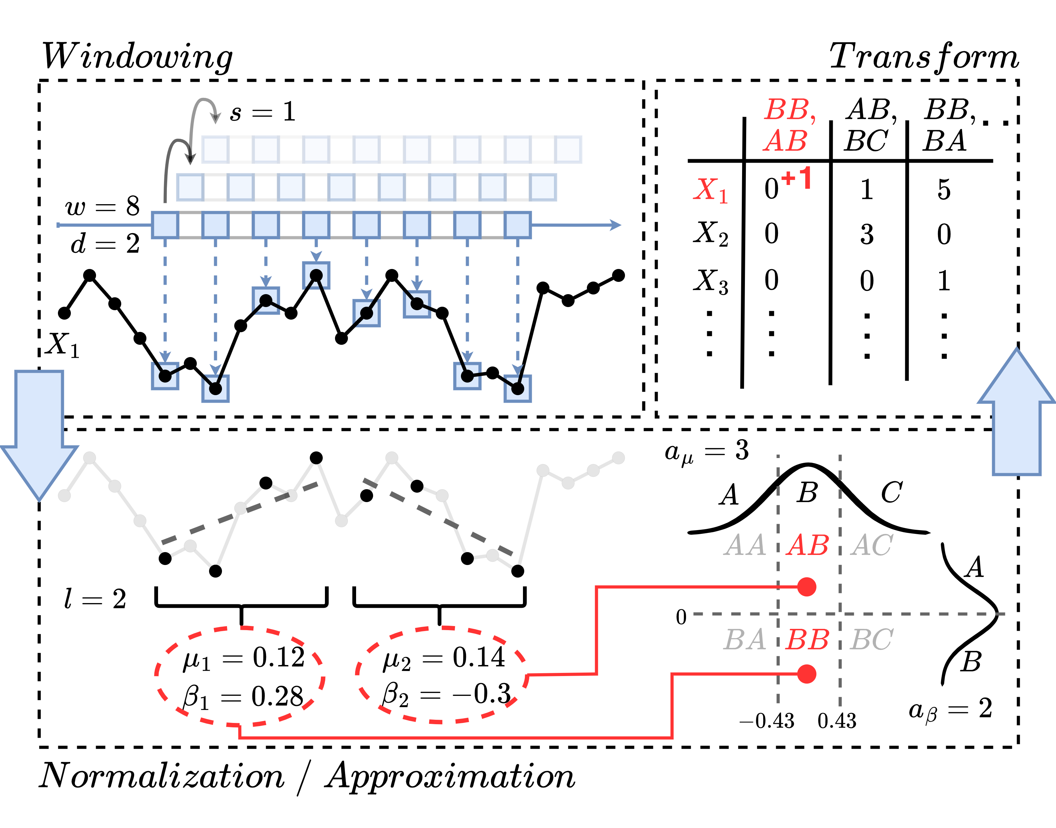
Figure 1: A simplified borf schema for a univariate time series ${X}_{1}$. A receptive field with size $8$ ($w=8$), dilation $2$ ($d=2$), and stride $1$ ($s=1$) is first extracted. Then, it is normalized and approximated using a modified version of 1d-sax (1d-sax-na), to obtain a pattern with a word length of 2 ($l=2)$, and using 3 symbols for the mean ($a_{\mu}=3$) and 2 for the slope ($a_{\beta}=2$). Finally, the borf representation is updated by adding $1$ to the number of times the pattern “$BB,AB$” was observed in ${X}_{1}$.

borf can be schematized into four steps: windowing, normalization, approximation, and transform, depicted in Figure 1, and presented in Algorithm 1. borf takes as input a time series dataset, $\mathcal{{X}}$, and outputs a Bag-of-Receptive-Fields ${P}$, using a few hyperparameters that define the characteristics of the extracted patterns. The first step is to initialize the empty Bag-Of-Receptive-Fields, ${P}$ (line 1). For building ${P}$, we use the sparse coordinate format (COO). In this format, the non-zero elements of a matrix are stored along with their corresponding row and column indices in a three-column matrix. This format is ideal in our setting where ${P}$ needs to be built incrementally. For ease of understanding, in Algorithm 1 and Figure 1, we represent this data structure as a single array, ${P}$. However, ${P}$ is never stored in its dense form to ensure space efficiency.

Once ${P}$ is initialized, borf iterates over each signal of each time series (lines 2-3) to divide it into equally-sized receptive fields (line 4). This is the windowing step, depicted in Figure 1 (top-left). Each receptive field is then standardized in the normalization step, using a threshold to identify constant segments (lines 5-6). The normalization ensures that the pattern’s scale does not influence its final symbolic representation. In the approximation step (line 7), the pattern is then discretized using a generalized version of 1d-sax, (1d-sax-na), and thus converted into a symbolic word (Figure 1, bottom). Finally, ${P}$ is updated in the transform step (lines 8-11) by checking if the retrieved word is already in ${P}$ (line 8). If that is the case, the Bag-of-Receptive-Fields entry is increased by $1$ (Figure 1, top-right, and line 9), else a new entry is created and set to $1$ (lines 10-11).

Algorithm 1 shows the training process for a single configuration of borf. We iterate this procedure $g$ times, changing hyperparameters to obtain patterns at multiple resolutions, i.e., receptive fields that capture different input signal properties. If two runs with different configurations yield the same pattern, they will be treated as two separate patterns with separate counts. In simple words, patterns from each configuration are independent, and the resulting borf representations are stacked horizontally: ${P}=\left[{P}_{1}\,|\,{P}_{2}\,|\,\ldots\,|\,{P}_{g}\right]$ . This allows for running the algorithm with multiple configurations in a parallel fashion. In the experimental section, we discuss parameters for the multiple resolutions and the algorithm’s complexity with empirical evidence of its scalability, showing its possible usage as an interpretable machine learning approach. All the steps are thoroughly explained in the following sections.

Windowing.

This step introduces a strided and dilated windowing approach to extract receptive fields. Dilation plays an essential role in convolution, offering control over receptive field size and determining the spacing between convolutional filter elements, enabling the capture of long-range dependencies and patterns. By introducing gaps between elements, dilation expands the receptive field and facilitates the incorporation of distant information. Via sliding window, we can extract a set of receptive fields, which capture different aspects of a time series at various levels of resolution. Formally, we define a windowize function that takes as input a signal x, and, by varying $j$, extracts a set of receptive fields ${R}={\textit{windowize}}(\textbf{x},w,d,s)$, with $j=1+i\cdot s$ and $0\leq i\leq\left\lfloor\nicefrac{{(m-w-(d-1)(w-1))}}{{s}}\right\rfloor$. The stride $s$ determines the displacement of the filter as it moves along the input data, allowing for downsampling and adjustment of output resolution. The receptive field definition generalizes the concept of subsequence, i.e., a subsequence obtained through a standard sliding window is a receptive field having $d=1$ and $s=1$.

Normalization.

For each extracted receptive field, $\textbf{r}\in{R}$, borf performs normalization through a thresholded standardization in the normalize function. Formally, given a single point $x$ of r:

$${\textit{normalize}}(x)=\dfrac{x-\mu_{\textbf{r}}}{\sigma_{\textbf{r}}}\cdot\textbf{1}\left[\dfrac{\sigma_{\textbf{r}}}{\sigma_{\textbf{x}}}\geq\theta\right]$$

where $\mu_{\textbf{r}}$ and $\sigma_{\textbf{r}}$ are the average and standard deviation of r, $\sigma_{\textbf{x}}$ is the standard deviation of the full signal, x, $0\leq\theta\leq 1$ is a threshold parameter, and 1 is the indicator function. This threshold avoids blowing up the noise of (almost) constant, receptive fields. If ${\sigma_{\textbf{r}}}/{\sigma_{\textbf{x}}}<\theta$, we assume the segment to be constant, and we directly set it to $0$. At this step, we deal with missing values through complete case analysis, ignoring them in the computation of the mean and standard deviation. If the receptive field, or even the full signal, lacks valid values, we leave the NaN vector as is.

Approximation.

Once the receptive fields are extracted and normalized, they can be converted to symbolic words through the 1d-sax-na function. We specifically chose 1d-sax as it is a standard generalization of sax, and for its linear complexity and easy interpretability. Given r, we first segment the receptive fields in $l$ segments containing $q=w/l$ points. Contrary to the original sax, in the case where $w$ is not divisible by $l$, we allow segments to have a slightly different number of observations. The edges indices are therefore computed as follows: $\textbf{e}=\left[1,\left\lfloor\nicefrac{{(w-1)}}{{{l}}}\right\rfloor+1,\left\lfloor\nicefrac{{(2w-1)}}{{l}}\right\rfloor+1,\ldots,\left\lfloor\nicefrac{{(lw-1)}}{{l}}\right\rfloor+1\right]\in\mathbb{N}^{l+1}$. The receptive field is divided then into a set of segments, $S=\{\textbf{r}_{e_{1}:e_{2}},\dots,\textbf{r}_{e_{l}:e_{l+1}}\}\in\dot{\mathbb{R}}^{l\times q}$, with their respective original time index, $T=\{\textbf{t}_{e_{1}:e_{2}},\dots,\textbf{t}_{e_{l}:e_{l+1}}\}\in{\mathbb{N}}^{l\times q}$. Given that each segment can possibly contain missing values, we generalize PLA through complete case analysis. For each of the (almost) equal-length segments, $\textbf{r}_{e_{i}:e_{i+1}}$ and $\textbf{t}_{e_{i}:e_{i+1}}$, (r and t for simplicity), we create an index vector, containing only the indices of valid values, i.e., $\textbf{i}=[i\mid r_{i}\neq\textit{NaN}]$. We can now perform a modified PLA via least squares. We compute the sample mean, iterating over the index vector i:

$$\mu=\begin{cases}|\textbf{i}|^{-1}\sum_{i\in\textbf{i}}x_{t_{i}}&\quad|\textbf{i}|\geq 1,\\ \textit{NaN}&\quad\textit{otherwise}.\end{cases}$$

Then, the slope can be computed as follows:

$$\beta=\begin{cases}\dfrac{\sum_{i\in\textbf{i}}(t_{i}-|\textbf{i}|^{-1}\sum_{i\in\textbf{i}}t_{i})(x_{t_{i}}-\mu)}{\sum_{i\in\textbf{i}}(t_{i}-|\textbf{i}|^{-1}\sum_{i\in\textbf{i}}t_{i})^{2}}&\quad|\textbf{i}|\geq 2,\\ 0&\quad|\textbf{i}|=1,\\ \textit{NaN}&\quad\textit{otherwise}.\end{cases}$$

In simple terms, the slope can be computed via PLA only if at least two valid observations exist in the segment. If only one valid value exists, the slope is set to zero. Finally, the slope and average are set to NaN if no valid value exists. At this point, we have two vectors, one containing the averages $\boldsymbol{\mu}=[{\mu}_{1},\dots,{\mu}_{l}]\in\dot{\mathbb{R}}^{l}$, and one containing the slopes, $\boldsymbol{\beta}=[\beta_{1},\dots,\beta_{l}]\in\dot{\mathbb{R}}^{l}$, of each segment of the receptive field. Values in each vector are then quantized using two separate alphabets, $\mathbb{{A}}_{\mu}$ and $\mathbb{{A}}_{\beta}$, containing $a_{\mu}\geq 2$ and $a_{\beta}\geq 1$ symbols, respectively. In practice, depending on their value, elements in the vectors are assigned a symbol. Specifically, the average values are quantized using $a_{\mu}$ symbols, obtained through the quantiles of the Gaussian distribution $\mathcal{N}(0,1)$, while the slope values are quantized on $a_{\beta}$ levels according to the quantiles of the Gaussian distribution $\mathcal{N}(0,\nicefrac{{0.03}}{{(w\cdot d)}})$, where $0.03$ is a scaling factor proposed by Malinowski et al., (2013) in the original 1d-sax paper, and $w\cdot d$ is the effective time-span adjusted by the dilation of the receptive field. Once quantized, the symbols are concatenated to form the final approximated receptive field $\textit{{1d-sax-na}}(\textbf{r},l,a_{\mu},a_{\beta})=[\textit{prefix},\tilde{\mu}_{1}\tilde{\beta}_{1},\dots,\tilde{\mu}_{l}\tilde{\beta}_{l}]=\tilde{\textbf{r}}\in\mathbb{A}^{l+1}$ with $|\mathbb{A}|=a_{\mu}\cdot a_{\beta}+1$, where the $+1$ counts for the symbol added for denoting $NaN$ average and slope values. The prefix contains the configuration and signal id, i.e., words extracted from different configurations and different time series signals are independent of each other. If $a_{\beta}=1$, 1d-sax-na reduces to standard sax.

Transform.

Given a newly created word, $\tilde{\textbf{r}}$, we need to store it. First, we check if $\tilde{\textbf{r}}$ already exists in ${P}$. If it does, i.e., $[*,\tilde{\textbf{r}}]\in P$, we increase the count in the entry ${P}[i,\tilde{\textbf{r}}]$ by $1$, where $i$ is the index of the time series we are processing. If, instead, the word was never observed, the update process differs at training and inference time. At training time, we initialize a new entry in ${P}[i,\tilde{\textbf{r}}]$ by setting it to $1$. At inference time, we can not consider it, given that it was never observed during training. In other words, at inference time, the algorithm only performs updates of ${P}$ for words found at training time, i.e., no new word is added in this phase. At the end of the algorithm, ${P}$ contains the overall count of appearances of each word in each time series. Thus, any model trained on this data will base its predictions on easily understandable features.

5 Experiments

Datasets.

We test borf on TSC and TSER on the full main repositories proposed in the literature. For TSC, we use the 158 datasets from the UCR and UEA TSC repositories (Bagnall et al.,, 2018; Dau et al.,, 2019), which contain 128 univariate and 30 multivariate datasets. For TSER, we use the UEA and UCR Time Series Extrinsic Regression Repository (Tan et al.,, 2020), which contains 19 datasets, 4 univariate, and 15 multivariate. We adopt the default training and test splits. Some datasets contain time series with a variable number of observations, and some contain missing values. For methods that do not support this kind of data, we apply missing value imputation by linear interpolation and last value padding. Further, we concatenate all signals in a single axis for algorithms that do not support multivariate time series.

BORF Hyperparameters.

Following the current trend in TSC and TSER (Tan et al.,, 2021; Ruiz et al.,, 2021), instead of fine-tuning borf to maximize performance for specific applications, we propose a model that achieves good results in a wide range of problems. Since several hyperparameters exist, we provide a heuristic that computes a vector of window sizes, dilations, and word lengths as follows: $\textbf{w}=[2^{2},2^{3},\dots,2^{\lfloor\log_{2}m\rfloor}]$, $\textbf{d}=[2^{0},2^{1},\dots,2^{\lfloor\log_{2}(\log_{2}m)\rfloor}]$, $\textbf{l}=[2^{0},2^{1},2^{2},2^{3}]$. Once these vectors are computed, each valid combination of elements is used as a configuration of borf, resulting in a multi-resolution representation of the time series. The stride is always set to $1$, $s=1$. We only tune the following $3$ parameters once for each task. For TSC we set $a_{\mu}=2$, $a_{\beta}=3$, and $\theta=0.15$. For TSER, $a_{\mu}=3$, $a_{\beta}=1$ and $\theta=0.05$.

After the transformation, many models can be used to perform supervised tasks. We focused on fast linear or tree-based approaches. From preliminary benchmarks on a subset of datasets, we found that linear models tend to perform best in TSC, while tree-based models are better suited for TSER. Linear models usually benefit from more normally-shaped features. For this reason, we apply an arcsinh function element-wise after the borf transform and before a linear-svc classifier with default parameters. For TSER, we use a LightGBM regressor with default parameters.

Competitors.

We compare borf against several state-of-the-art approaches presented in Section 2. For TSC, as a common baseline, we use KNN with DTW as distance and a Sakoe-Chiba band of $0.1$ (knn-dtw). For competitor dictionary-based approaches, we test bop, sax-vsm, mr-sqm, a boss ensemble, and muse. For interval-base approaches, we use Time Series Bag of Features (tsbf), Time Series Forest (tsf), and Canonical Interval Forest (cif). For shapelet-based, we benchmark Random Shapelet Forest (rsf) and the standard Shapelet Transform (st). Finally, we also compare against rocket. For TSER, there are fewer choices, and we benchmark all of the previous that can be directly applied to TSER, i.e., knn-dtw, bop, tsf, sf, and rocket. We also directly test a LightGBM regressor (lgbm) on the raw time series. All models are trained with the default library hyperparameters or values proposed in the respective papers. Each model is allowed approximately one week ($10,000$ minutes) for training and inference on each dataset, and is allocated $256GB$ of memory. A run is considered failed if it exceeds the maximum time or crashes due to out-of-memory errors. Each benchmark is performed $3$ times with different seeds for models with a random component, and the average performance is taken.

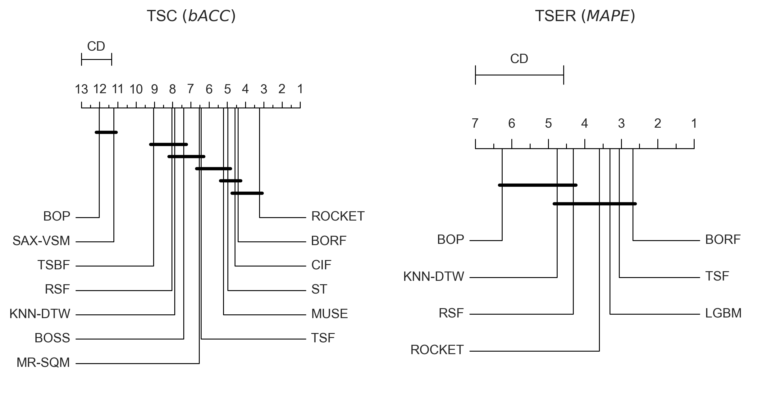
Figure 2: CD diagram for TSC in terms of bACC (left), and for TSER in terms of MAPE (right). Best models to the right.

Results.

The comparison of the ranks of all methods against each other considering all datasets is presented in Figure 2 with Critical Difference (CD) diagrams (Demsar,, 2006). Two methods are tied if the null hypothesis that their performance is the same cannot be rejected using the Nemenyi test at $\alpha{=}0.05$. The performance metric used for TSC is Balanced Accuracy (bACC) (Brodersen et al.,, 2010), which accounts for both false positives and false negatives when dealing with imbalanced data. For TSER, we adopt Mean Absolute Percentage Error (MAPE). In both plots, best values have lower ranks and appear on the right-hand side. For TSC, borf scores second place and is statistically tied to rocket. Notably, borf outperforms significantly SAX-based methods such as mr-sqm and sax-vsm, and is the best-performing dictionary-based approach. For TSER, borf is the overall best approach, outperforming even state-of-the-art black-box competitors. It is interesting to see that lgbm, which does not consider the sequentiality of data, outperforms every other method, except borf and tsf. A similar observation was made in (Tan et al.,, 2021), highlighting the need for more research for this task. Another issue is the lack of big repositories for TSER, which produces a CD plot that cannot definitively separate the top-performing approaches.

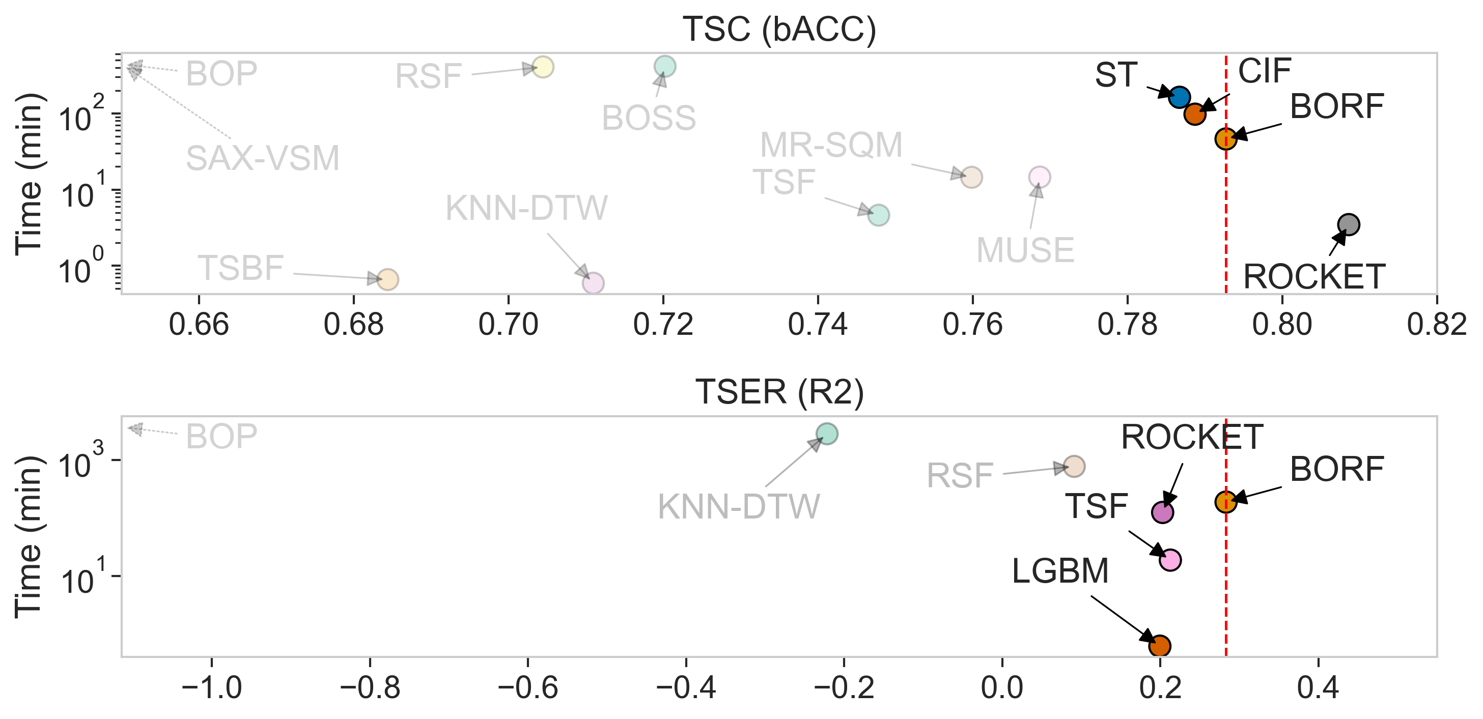
Figure 3: Mean performance and training time between borf and competitors for TSC (top) and TSER (bottom). Best models to the right.

For this reason, we also present a performance versus time comparison in Figure 3 (less competitive approaches are shaded). The x-axis shows the mean performance of the models, in terms of bACC for TSC, and R2 for TSER. Therefore, the best-performing models are on the right. On the y-axis is the training time in minutes. Thus, faster approaches are at the bottom. Regarding TSC, the overall best approach is rocket, while cif and st are close to borf but are also slower. We highlight that while rocket performs better in TSC, it is also a black-box, completely opaque from a human standpoint. In TSER, borf is the best-performing method. lgbm, tsf, and rocket are the only comparable ones, with a noticeable performance gap. In that group lgbm performs comparably to tsf and rocket, while being notably faster. In general, while borf exhibits average training runtimes, it is also the only approach that offers competitive performance while being deterministic, which is a crucial feature for XAI purposes. Additionally, it is worth noting that because not all approaches support parallel computation, runtimes are recorded using a single thread to ensure better comparability. These results represent worst-case scenarios, and many of the benchmarked approaches, including borf, can be significantly accelerated through multiprocessing.

Complexity and Scalability.

The complexity of borf is dominated by that of 1d-sax-na, which for a sequence of $w$ points is linear, i.e., $O(w)$ (Malinowski et al.,, 2013). For a single signal, 1d-sax-na has to be performed one time for each receptive field, i.e., $\left\lfloor\nicefrac{{(m-w-(d-1)(w-1))}}{{s}}\right\rfloor+1$ times. The worst case scenario is when $d=1$, $s=1$, and $w=\nicefrac{{(m+1)}}{{2}}$. Applied to the full dataset and repeated for $g$ configurations, the time complexity of borf is $O(g\cdot n\cdot c\cdot m^{2})$.

Regarding space complexity, there are two aspects to consider. First, the number of possible extracted words for a given configuration depends on the word length, $l$, and alphabet size, $a$, and is exponential, $O(a^{l})$. However, there cannot be more words than receptive fields. Thus, in the worst case scenario, when there are no duplicate words, the complexity is $O(g\cdot c\cdot\min(a^{l},n\cdot m^{2}))$. Given the proposed heuristic, the effective number of receptive fields is at least one order of magnitude smaller than this bound, as shown in Figure 4 (left). For each dataset, Figure 4 (left) shows the number of time series points (x-axis) versus the number of extracted patterns (y-axis, blue) and the theoretical maximum of extractable patterns (y-axis, orange). In particular, the empirical space complexity is linear w.r.t. the number of points and very close to $n\cdot c\cdot m$. Further, as shown in Figure 4 (right), the density (x-axis) of the borf representation naturally decreases as the number of features increases (y-axis), with the density, $\rho$, being defined as the ratio between the number of non-zero entries w.r.t. the number of entries in ${P}$, $\rho=\textit{nnz}({P})/|{P}|$. Models developed for this kind of representation tend to be more efficient as the number of features increases, exploiting the increasingly lower proportion of non-zero elements in the input matrix (Pedregosa et al.,, 2011).

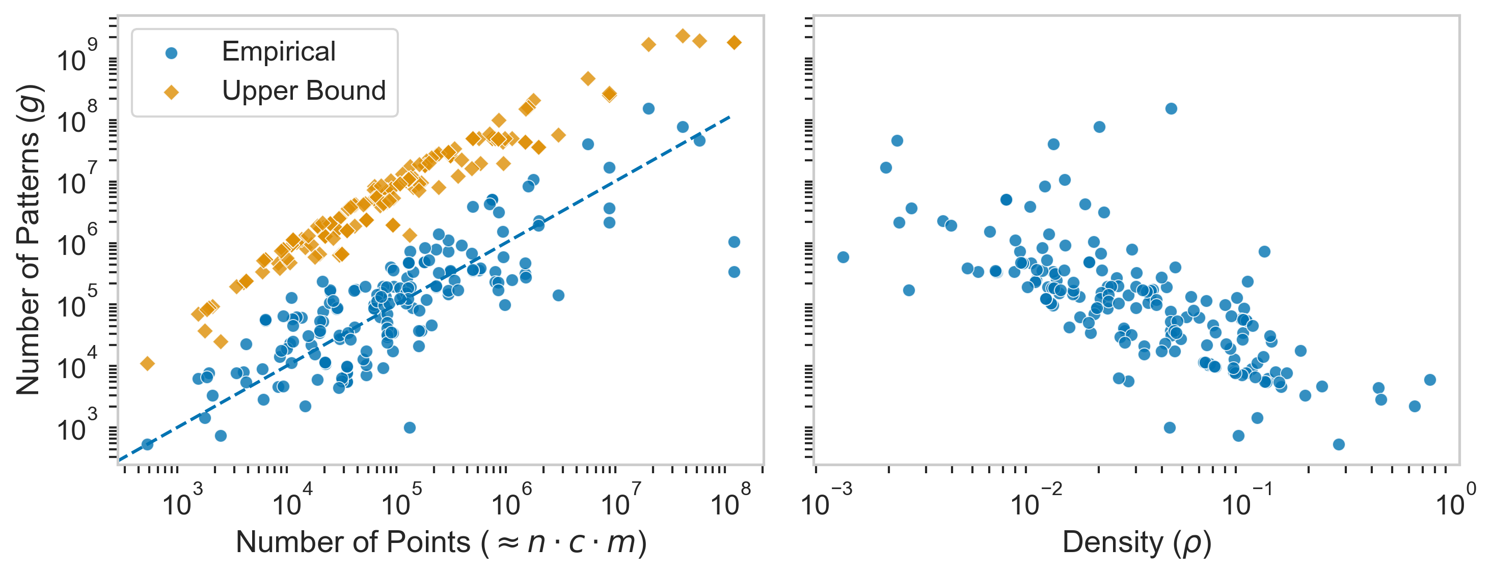
Figure 4: Number of points against extracted patterns (left). Density against number of patterns (right).

Interpretability.

Here we show how a feature-based explanation can be partially mapped to a saliency map in an borf representation. Given a time series, ${X}$, its borf conversion, p, and a feature importance vector, $\boldsymbol{\phi}$, obtained through some local explainer, such as SHAP (Lundberg and Lee,, 2017), we propose a way to build a saliency map, $\Psi$. A single feature importance, $\phi_{i}$, for a single symbolic pattern, $p_{i}$, can be mapped back to the original timesteps only if $p_{i}$ is contained in the time series, i.e., $p_{i}>0$. If that is the case, we can retrieve the multiset $T_{i}=\{(k_{1},j_{1}),(k_{2},j_{2}),\dots\}$, containing all the alignment indices, possibly duplicate, for $p_{i}$. The saliency matrix is then defined as $\Psi^{*}=[\psi_{1,1},\dots,\psi_{c,m}]\in\mathbb{R}^{c\times m}$, where $\psi_{k,j}=\sum_{i=1}^{h}\phi_{i}\cdot|\{(k,j)\in T_{i}\}|.$ To obtain the final saliency map, $\Psi^{*}$ is multiplied by a scaling factor:

$$\Psi=\Psi^{*}\cdot\frac{\sum_{i=1}^{h}{\phi_{i}\cdot\textbf{1}[p_{i}>0]}}{\sum_{k=1}^{c}\sum_{j=1}^{m}{\psi_{k,j}}}$$

In practice, the sum of the saliency values is scaled to equal the sum of the feature importances of contained patterns. Hence, the final explanation comprises a saliency map explaining the contained patterns, and a feature importance vector, explaining the contribution of not-contained patterns.

In Figure 5, we show an example of such an explanation on one of the most challenging and novel tasks from an interpretability standpoint, i.e., multivariate TSER. The time series is from the HouseholdPowerConsumption1 dataset, containing $5$ signals of the minutely voltage, current and sub-meter energy of a house near Paris, France (Hebrail and Berard,, 2012). The task is to predict the global active power in kiloWatt (kW), and the prediction of borf ($1460.4kW$) is extremely close to the real one ($1460.9kW$). The feature importance vector of p is obtained through SHAP. In Figure 5 (left), the multivariate time series is shown, and each point is colored based on its importance. Positive SHAP values (red) indicate that the observation “pushes” the prediction toward higher active power, while negative values indicate lower power consumption. Values close to $0$ are not relevant to the prediction. On the right, we show each signal’s most important not-contained patterns, i.e., $p_{i}=0$, colored based on their contribution toward the prediction. These shapes are obtained by averaging all the receptive fields corresponding to a specific SAX word, for each instance of the training set. At first glance, it is easy to see that the most important signals for the regression are sub-meter energy 2 and 3 ($SubMt_{2}$ and $SubMt_{3}$), followed by the current ($Amp$). Voltage ($Volt$) and $SubMt_{1}$ are almost all gray, so they do not contribute significantly toward the prediction. From a layman’s point of view, it seems that rapid increases in sub-meter energy ($SubMt_{2}$, $SubMt_{3}$) are indicators of an increase in consumption. Further, the most important pattern for $SubMt_{2}$ is “U-shaped”, and its absence strongly indicates increased active power. $SubMt_{3}$ mainly pushes the prediction toward lower power consumption, and the not-contained patterns are harder to interpret, having a higher frequency. In this case, the explanation is more technical and requires a domain expert.

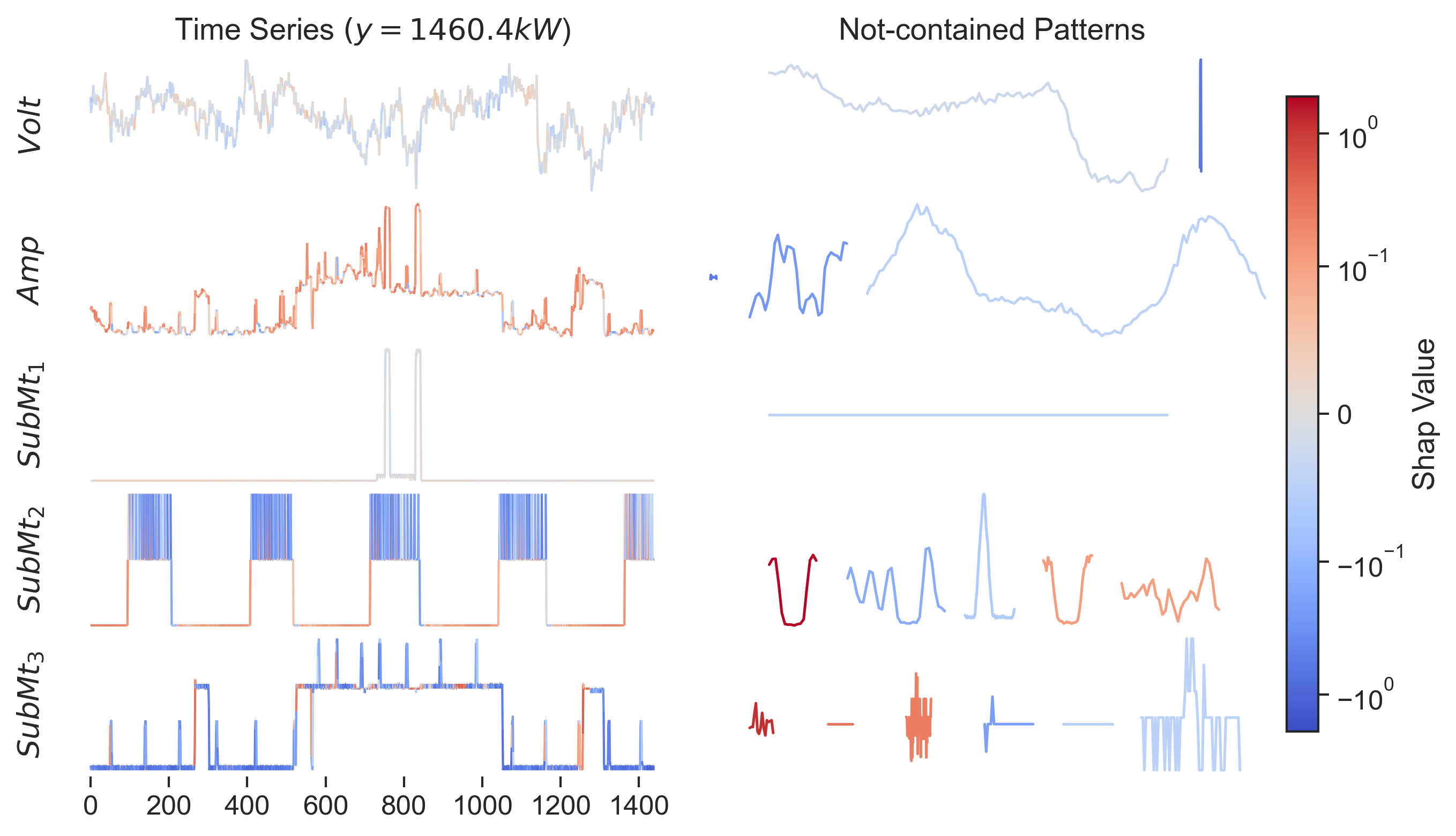
Figure 5: A saliency and feature-based explanation on a multivariate time series of the HouseholdPowerConsumption1 dataset. (left) original time series; (right) most important not-contained patterns. The more intense the color, the more important the feature.

6 Conclusion

We have presented borf, a Bag-Of-Receptive-Fields deterministic transform that, by incorporating time series convolution operators and 1d-sax, addresses the limitations of existing TSA techniques, offering improved performance, interpretability, and applicability in real-world scenarios. We evaluated borf on TSC and TSER tasks, showcasing its superior performance in TSER and competitive results in TSC. Additionally, we outlined how borf can be used to achieve saliency and feature-based explanations. A limitation of borf for very big datasets is the quadratic time complexity w.r.t. the number of observations. For future research directions, we plan on exploring the stride parameter to achieve lower running times without sacrificing performance. Further, we plan on extending univariate receptive fields to multivariate ones to generate symbolic words that can span more than one signal. Regarding data, the next natural obstacle is being able to deal with unequally sampled time series in which the time dimension is not constant. Finally, we plan on extending borf to achieve interpretable time series forecasting and test it on unsupervised tasks like clustering and anomaly detection.

References

- Bagnall et al., (2018) Bagnall, A., Dau, H. A., Lines, J., Flynn, M., Large, J., Bostrom, A., Southam, P., and Keogh, E. (2018). The uea multivariate time series classification archive, 2018. arXiv preprint arXiv:1811.00075.
- Bagnall et al., (2017) Bagnall, A., Lines, J., Bostrom, A., Large, J., and Keogh, E. (2017). The great time series classification bake off: a review and experimental evaluation of recent algorithmic advances. Data mining and knowledge discovery, 31:606–660.
- Baydogan et al., (2013) Baydogan, M. G., Runger, G., and Tuv, E. (2013). A bag-of-features framework to classify time series. IEEE transactions on pattern analysis and machine intelligence, 35(11):2796–2802.
- Bodria et al., (2023) Bodria, F., Giannotti, F., Guidotti, R., Naretto, F., Pedreschi, D., and Rinzivillo, S. (2023). Benchmarking and survey of explanation methods for black box models. Data Mining and Knowledge Discovery, pages 1–60.
- Brodersen et al., (2010) Brodersen, K. H., Ong, C. S., Stephan, K. E., and Buhmann, J. M. (2010). The balanced accuracy and its posterior distribution. In 2010 20th international conference on pattern recognition, pages 3121–3124. IEEE.
- Dau et al., (2019) Dau, H. A., Bagnall, A., Kamgar, K., Yeh, C.-C. M., Zhu, Y., Gharghabi, S., Ratanamahatana, C. A., and Keogh, E. (2019). The ucr time series archive. IEEE/CAA Journal of Automatica Sinica, 6(6):1293–1305.
- Dempster et al., (2020) Dempster, A., Petitjean, F., and Webb, G. I. (2020). Rocket: exceptionally fast and accurate time series classification using random convolutional kernels. Data Mining and Knowledge Discovery, 34(5):1454–1495.
- Demsar, (2006) Demsar, J. (2006). Statistical comparisons of classifiers over multiple data sets. J. Mach. Learn. Res., 7:1–30.
- Deng et al., (2013) Deng, H., Runger, G., Tuv, E., and Vladimir, M. (2013). A time series forest for classification and feature extraction. Information Sciences, 239:142–153.
- Flynn et al., (2019) Flynn, M., Large, J., and Bagnall, T. (2019). The contract random interval spectral ensemble (c-rise): the effect of contracting a classifier on accuracy. In Hybrid Artificial Intelligent Systems: 14th International Conference, HAIS 2019, León, Spain, September 4–6, 2019, Proceedings 14, pages 381–392. Springer.
- Hebrail and Berard, (2012) Hebrail, G. and Berard, A. (2012). Individual household electric power consumption. UCI Machine Learning Repository. DOI: https://doi.org/10.24432/C58K54.
- Hills et al., (2014) Hills, J., Lines, J., Baranauskas, E., Mapp, J., and Bagnall, A. (2014). Classification of time series by shapelet transformation. Data mining and knowledge discovery, 28:851–881.
- Hung and Anh, (2007) Hung, N. Q. V. and Anh, D. T. (2007). Combining sax and piecewise linear approximation to improve similarity search on financial time series. In 2007 International Symposium on Information Technology Convergence (ISITC 2007), pages 58–62. IEEE.
- Karlsson et al., (2016) Karlsson, I., Papapetrou, P., and Boström, H. (2016). Generalized random shapelet forests. Data mining and knowledge discovery, 30:1053–1085.
- Keogh et al., (2001) Keogh, E., Chakrabarti, K., Pazzani, M., and Mehrotra, S. (2001). Dimensionality reduction for fast similarity search in large time series databases. Knowledge and information Systems, 3:263–286.
- Kreindler and Lumsden, (2006) Kreindler, D. M. and Lumsden, C. J. (2006). The effects of the irregular sample and missing data in time series analysis. Nonlinear dynamics, psychology, and life sciences, 10(2):187–214.
- Le Nguyen et al., (2019) Le Nguyen, T., Gsponer, S., Ilie, I., O’reilly, M., and Ifrim, G. (2019). Interpretable time series classification using linear models and multi-resolution multi-domain symbolic representations. Data mining and knowledge discovery, 33:1183–1222.
- Lin et al., (2007) Lin, J., Keogh, E., Wei, L., and Lonardi, S. (2007). Experiencing sax: a novel symbolic representation of time series. Data Mining and knowledge discovery, 15:107–144.
- Lin et al., (2012) Lin, J., Khade, R., and Li, Y. (2012). Rotation-invariant similarity in time series using bag-of-patterns representation. Journal of Intelligent Information Systems, 39:287–315.
- Lines et al., (2012) Lines, J., Davis, L. M., Hills, J., and Bagnall, A. (2012). A shapelet transform for time series classification. In Proceedings of the 18th ACM SIGKDD international conference on Knowledge discovery and data mining, pages 289–297.
- Lundberg and Lee, (2017) Lundberg, S. M. and Lee, S.-I. (2017). A unified approach to interpreting model predictions. Advances in neural information processing systems, 30.
- Malinowski et al., (2013) Malinowski, S., Guyet, T., Quiniou, R., and Tavenard, R. (2013). 1d-sax: A novel symbolic representation for time series. In Advances in Intelligent Data Analysis XII: 12th International Symposium, IDA 2013, London, UK, October 17-19, 2013. Proceedings 12, pages 273–284. Springer.
- Middlehurst et al., (2020) Middlehurst, M., Large, J., and Bagnall, A. (2020). The canonical interval forest (cif) classifier for time series classification. In 2020 IEEE international conference on big data (big data), pages 188–195. IEEE.
- Nguyen and Ifrim, (2022) Nguyen, T. L. and Ifrim, G. (2022). Fast time series classification with random symbolic subsequences. In International Workshop on Advanced Analytics and Learning on Temporal Data, pages 50–65. Springer.
- Pedregosa et al., (2011) Pedregosa, F., Varoquaux, G., Gramfort, A., Michel, V., Thirion, B., Grisel, O., Blondel, M., Prettenhofer, P., Weiss, R., Dubourg, V., Vanderplas, J., Passos, A., Cournapeau, D., Brucher, M., Perrot, M., and Duchesnay, E. (2011). Scikit-learn: Machine learning in Python. Journal of Machine Learning Research, 12:2825–2830.
- Ruiz et al., (2021) Ruiz, A. P., Flynn, M., Large, J., Middlehurst, M., and Bagnall, A. (2021). The great multivariate time series classification bake off: a review and experimental evaluation of recent algorithmic advances. Data Mining and Knowledge Discovery, 35(2):401–449.
- Schäfer, (2015) Schäfer, P. (2015). The boss is concerned with time series classification in the presence of noise. Data Mining and Knowledge Discovery, 29:1505–1530.
- Schäfer and Högqvist, (2012) Schäfer, P. and Högqvist, M. (2012). Sfa: a symbolic fourier approximation and index for similarity search in high dimensional datasets. In Proceedings of the 15th international conference on extending database technology, pages 516–527.
- Schäfer and Leser, (2017) Schäfer, P. and Leser, U. (2017). Multivariate time series classification with weasel+ muse. arXiv preprint arXiv:1711.11343.
- Senin and Malinchik, (2013) Senin, P. and Malinchik, S. (2013). Sax-vsm: Interpretable time series classification using sax and vector space model. In 2013 IEEE 13th international conference on data mining, pages 1175–1180. IEEE.
- Shumway et al., (2000) Shumway, R. H., Stoffer, D. S., and Stoffer, D. S. (2000). Time series analysis and its applications, volume 3. Springer.
- Spinnato et al., (2022) Spinnato, F., Guidotti, R., Nanni, M., Maccagnola, D., Paciello, G., and Farina, A. B. (2022). Explaining crash predictions on multivariate time series data. In International Conference on Discovery Science, pages 556–566. Springer.
- Tan et al., (2020) Tan, C. W., Bergmeir, C., Petitjean, F., and Webb, G. I. (2020). Monash university, uea, ucr time series extrinsic regression archive. arXiv preprint arXiv:2006.10996.
- Tan et al., (2021) Tan, C. W., Bergmeir, C., Petitjean, F., and Webb, G. I. (2021). Time series extrinsic regression: Predicting numeric values from time series data. Data Mining and Knowledge Discovery, 35:1032–1060.
- Theissler et al., (2022) Theissler, A., Spinnato, F., Schlegel, U., and Guidotti, R. (2022). Explainable ai for time series classification: A review, taxonomy and research directions. IEEE Access.
- Ye and Keogh, (2011) Ye, L. and Keogh, E. (2011). Time series shapelets: a novel technique that allows accurate, interpretable and fast classification. Data mining and knowledge discovery, 22:149–182.