Filtered Semi-Markov CRF

Abstract

Semi-Markov CRF has been proposed as an alternative to the traditional Linear Chain CRF for text segmentation tasks such as Named Entity Recognition (NER). Unlike CRF, which treats text segmentation as token-level prediction, Semi-CRF considers segments as the basic unit, making it more expressive. However, Semi-CRF suffers from two major drawbacks: (1) quadratic complexity over sequence length, as it operates on every span of the input sequence, and (2) inferior performance compared to CRF for sequence labeling tasks like NER. In this paper, we introduce Filtered Semi-Markov CRF, a variant of Semi-CRF that addresses these issues by incorporating a filtering step to eliminate irrelevant segments, reducing complexity and search space. Our approach is evaluated on several NER benchmarks, where it outperforms both CRF and Semi-CRF while being significantly faster. The implementation of our method is available on Github.

1 Introduction

Sequence segmentation, the process of dividing a sequence into distinct, non-overlapping segments, has various applications, including Named Entity Recognition and Chinese Word Segmentation Tjong Kim Sang and De Meulder (2003); Li and Yuan (1998). In the past, this task has been approached as a sequence labeling problem using pre-defined templates, such as the BIO and BILOU schemes Ratinov and Roth (2009). The Conditional Random Field (CRF) Lafferty et al. (2001) has become a popular method for sequence labeling problems due to its ability to model the dependency between adjacent token tags. However, the CRF model may not efficiently capture the underlying structure of the sequence, as it is limited to modeling relationships between individual tokens rather than segments.

The Semi-Markov CRF Sarawagi and Cohen (2005) has been proposed as a variant of the CRF, allowing for the incorporation of higher-level segment features, such as segment width. While the Semi-CRF allows for a more natural approach to sequence segmentation, it suffers from slower learning and inference due to its quadratic complexity with respect to the sequence length. Additionally, the Semi-CRF often underperforms CRF, showing only marginal improvements in some cases Liang (2005); Daumé and Marcu (2005); Andrew (2006), which can be attributed to the Semi-CRF’s significantly larger solution space, complicating the search for optimal solutions.

To address the limitations of Semi-CRF, we propose Filtered Semi-CRF, which introduces a filtering step to prune irrelevant segments using a lightweight local segment classifier. By leveraging transformer-based features, such as BERT (Devlin et al., 2019), this classifier can identify high-quality candidate segments. Consequently, the task of the Semi-CRF is simplified to selecting the best segments from the pool of high-quality candidates. Our experiments demonstrate that this filtering step not only accelerates the decoding process but also improves the overall model performance.

Although pruning techniques have been applied to accelerate parsing algorithms (Roark and Hollingshead, 2008; Bodenstab et al., 2011), they often involve a trade-off between accuracy and inference speed. In contrast, our filtering approach is learned jointly and collaboratively with the Semi-CRF during training, resulting in a model that not only increases efficiency but also improves overall performance.

When evaluated on Named Entity Recognition, our model significantly outperforms both the CRF and Semi-CRF, achieving F1 score improvements of up to 2.5 and 1.1 points, respectively, on the CoNLL 2003 dataset. Additionally, our model also accelerates the decoding process to a speed that can be up to 20 times and 137 times faster than CRF and Semi-CRF, respectively.

2 Background

2.1 Probabilistic structured predictor

In this paper, we aim to produce a structured output ${\bm{y}}$ given an input sequence ${\bm{x}}$. To assess the compatibility between the input and output, we employ a parameterized score function ${\bm{S}}_{\theta}({\bm{y}}|{\bm{x}})$. The probability of a structure ${\bm{y}}$ given ${\bm{x}}$ is computed as follows:

$$p_{\theta}({\bm{y}}|{\bm{x}})=\frac{\exp{\bm{S}}_{\theta}({\bm{y}}|{\bm{x}})}{\sum_{{\bm{y}}^{\prime}\in\mathcal{Y}({\bm{x}})}\exp{\bm{S}}_{\theta}({\bm{y}}^{\prime}|{\bm{x}})}$$ (1)

where $\mathcal{Y}({\bm{x}})$ represents the set of all possible outputs for ${\bm{x}}$, and the denominator serves as a normalization constant, referred to as the partition function, denoted by $\mathcal{Z}_{\theta}({\bm{x}})$.

Training

During training, the goal is to update the model’s parameters $\theta$ to maximize the likelihood of the training data. The loss function for a pair of data points $({\bm{x}},{\bm{y}})$ is computed as follows:

$$\begin{split}\mathcal{L}({\bm{x}},{\bm{y}})&=-\log p_{\theta}({\bm{y}}|{\bm{x}})\\ &=-{\bm{S}}_{\theta}({\bm{y}}|{\bm{x}})+\log\mathcal{Z}_{\theta}({\bm{x}})\end{split}$$ (2)

This loss function can be optimized using a stochastic gradient descent algorithm on the training data. Computing the partition function $\mathcal{Z}_{\theta}({\bm{x}})$ can be challenging when the output space is large, but it can be calculated efficiently using dynamic programming in some cases.

Inference

During inference, the goal is to produce the most likely output:

$${\bm{y}}^{*}=\operatorname*{arg\,max}_{{\bm{y}}\in\mathcal{Y}({\bm{x}})}{\bm{S}}_{\theta}({\bm{y}}|{\bm{x}})$$ (3)

All the models we present in this paper follow this type of probabilistic modeling. For the remainder of this paper, we omit the dependency on $\theta$ for better readability.

2.2 Linear Chain CRF

The Linear-Chain CRF (Lafferty et al., 2001) is a sequence labeling model that assigns a label to each token in the input sequence, taking into account dependencies between adjacent labels. The score function of the CRF has the following form:

$${\bm{S}}({\bm{y}}|{\bm{x}})=\sum_{i=1}^{|{\bm{x}}|}\bm{\psi}(y_{i}|{\bm{x}})+\sum_{i=2}^{|{\bm{x}}|}{\bm{T}}[y_{i-1},y_{i}]$$ (4)

Here, $\bm{\psi}(y_{i}|{\bm{x}})\in\mathbb{R}$ is the sequence label score at position $i$, and ${\bm{T}}\in\mathbb{R}^{|Y|\times|Y|}$ is a learnable label transition matrix. The partition function is computed using the Forward algorithm and the Viterbi algorithm (Rabiner, 1989) is used to determine the optimal labeling, both with a computational complexity of $\mathcal{O}(L|Y|^{2})$ (More details in Appendix A.2).

2.3 Semi-Markov CRF

The Semi-CRF, proposed by (Sarawagi and Cohen, 2005), operates at the segment level and allows for the modeling of features that cannot be captured by traditional linear-chain CRFs. It produces a segmentation ${\bm{y}}$ of length $M$ for an input sequence ${\bm{x}}$ of length $L$ ($L\geq M$). A segmentation ${\bm{y}}=\{s_{1},\ldots,s_{M}\}\in\mathcal{Y}({\bm{x}})$ satisfies the following properties:

• Each segment $s_{k}=(i_{k},j_{k},l_{k})\in{\bm{y}}$ consists of a start position $i_{k}$, an end position $j_{k}$, and a label $l_{k}\in Y$.

• The segments have positive lengths and completely cover the input sequence positions $1,\ldots,L$ without overlapping. In other words, the start and end positions satisfy $i_{1}=1$, $j_{M}=L$, and for every $j_{k}$ and $i_{k}$ we have $1\leq i_{k}\leq j_{k}\leq L$, and $i_{k+1}=j_{k}+1$.

Consider a sentence from a Named Entity Recognition (NER) task: "Alain Farley works at McGill University". It would be segmented as ${\bm{y}}$=[(1,2,PER), (3,3,O), (4,4,O), (5,6,ORG)], considering assumption from Sarawagi and Cohen (2005) that non-entity segments (referred to as O or null segments) have unit length. Furthermore, the Semi-CRF score function is defined as follows:

$${\bm{S}}({\bm{y}}|{\bm{x}})=\sum_{k=1}^{M}\bm{\phi}(s_{k}|{\bm{x}})+{\bm{T}}[l_{k-1},l_{k}]$$ (5)

Here, $\bm{\phi}(s_{k}|{\bm{x}})\in\mathbb{R}$ represents the score of the $k$-th segment of ${\bm{y}}$, and ${\bm{T}}[l_{k-1},l_{k}]$ denotes the label transition score. Additionally, ${\bm{T}}[l_{0},l_{1}]=0$. The partition function of the Semi-CRF can be computed in polynomial time using a modified version of the Forward algorithm and the segmental Viterbi algorithm is used to compute optimal segmentation (Appendix A.3 for details). The computational complexity of the Semi-CRF increases quadratically with both the sequence length and the number of labels, i.e $\mathcal{O}(L^{2}|Y|^{2})$.

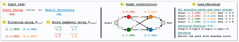
Figure 1: Filtered Semi-CRF for NER. The model takes as text sequence and output the best entity segments.

2.4 Graph-based Formulation of Semi-CRF

In this section, we present a graph-based formulation of the Semi-CRF. As explained in § 2.3 , a sequence ${\bm{x}}$ of length $L$ is divided into $M$ labeled segments $(i_{k},j_{k},l_{k})$, with $i_{k}$, $j_{k}$ and $l_{k}$ denoting respectively the start position, end position and the label. We define a directed graph $\mathcal{G}(V_{\text{full}},E)$, with $V_{\text{full}}$ its set of nodes composed of all possible segments $s_{k}$ of ${\bm{x}}$:

$$V_{\text{full}}=\bigcup_{i=1}^{L}\bigcup_{j=i}^{L}\bigcup_{l=1}^{\left|Y\right|}\{(i,j,l)\},$$ (6)

and an edge $s_{k^{\prime}}\rightarrow s_{k}\in E$ exists if and only if the start position of $s_{k}$ immediately follows the end position of $s_{k^{\prime}}$, i.e., $j_{k^{\prime}}+1=i_{k}$. The weight of an edge $s_{k^{\prime}}\rightarrow s_{k}$ is defined as:

$$w(s_{k^{\prime}}\rightarrow s_{k}|{\bm{x}})=\phi(s_{k}|{\bm{x}})+{\bm{T}}[l_{k^{\prime}},l_{k}],$$ (7)

where $\phi(s_{k}|{\bm{x}})$ is the score of the segment $s_{k}$ and ${\bm{T}}[l_{k^{\prime}},l_{k}]$ is the label transition score. Moreover, Any directed path ${s_{1},s_{2},\ldots,s_{M}}$ of the graph $\mathcal{G}$ corresponds to a valid segmentation of ${\bm{x}}$ if it verifies the segmentation properties described in § 2.3 . Additionally, the score of a valid path is computed as the sum of the edge scores, and is equivalent to the Semi-CRF score of the segmentation (Eq. 5):

The search for the best segmentation of the sequence ${\bm{x}}$ is equivalent to finding the maximal weighted path of the graph $\mathcal{G}$ that starts at $i_{1}=1$ and ends at $j_{M}=L$. This search can be done using a generic shortest path algorithm such as Bellman-Ford, whose complexity is of $L^{3}$. Nevertheless, taking into account the lattice structure of the problem, the Viterbi algorithm (Viterbi, 1967; Rabiner, 1989) can achieve this while reducing the complexity to $L^{2}$.

3 Filtered Semi-Markov CRF

In this section, we propose an alternative model to Semi-CRF, named Filtered Semi-CRF, which aims to address two fundamental weaknesses of the original model. First, the Semi-CRF is not well-suited for long texts due to its quadratic complexity and the prohibitively large search space. Secondly, in tasks such as Named Entity Recognition (NER), where certain segments are labeled as null (representing non-entity segments), the Semi-CRF graph can create multiple redundant paths, all leading to the same set of entities. For instance, consider the scenario described in § 2.3. In this scenario, multiple segmentations, such as ${\bm{y}}$=[(1,2,PER), (3,3,O), (4,4,O), (5,6,ORG)] or ${\bm{y}}$=[(1,2,PER), (3,4,O), (5,6,ORG)], would yield the same final set of labeled entities, specifically (1,2, PER) and (5,6,ORG) in this case. To remedy these shortcomings, our proposed model incorporates a filtering step that eliminates irrelevant segments using a lightweight local classifier. By leveraging transformer-based features, this classifier effectively selects high-quality candidate segments, significantly reducing the task of the Semi-CRF to merely choosing the best among already high-quality candidates.

3.1 Filtering

Local classifier

We first define the local classifier $\phi_{\text{local}}$ as a model that assigns a score to a labelled segment $s=(i,j,l)$ given an input sequence $\mathbf{x}$:

$$\phi_{\text{local}}(s=(i,j,l)|{\bm{x}})={{\bm{w}}_{l}}^{T}f({\bm{h}}_{i},\ldots,{\bm{h}}_{j})$$ (9)

where $\mathbf{h}_{i}\in\mathbb{R}^{D}$ is the token representation at position $i$ (computed by a pretrained transformer such as BERT), and $\mathbf{w}_{l}\in\mathbb{R}^{D}$ is a learnable weight associated with the label $l$. The function $f$ represents the segment featurizer, which aggregates token representations into a single feature representation. We found that a simple sum operation provides strong performance across settings.

Filtered graph

The filtering consists in removing the segments $s_{k}=(i_{k},j_{k},l_{k})$ for which $l_{k}=\operatorname*{arg\,max}_{l}\phi_{local}(i_{k},j_{k},l|x)$ and $l_{k}=\texttt{null}$:

This new set of filtered nodes $V$ requires to define the set of edges $E$ differently from the definition of § 2.4. Thus, we propose to define the edges following Liang et al. (1991): $\forall(s_{k^{\prime}},s_{k})\in V^{2}$, $s_{k^{\prime}}\rightarrow s_{k}\in E$ if $j_{k^{\prime}}<i_{k}$ and there is no $s_{k^{*}}\in V$ such that $j_{k^{\prime}}<i_{k^{*}}$ and $i_{k^{*}}<j_{k}$. This definition means that $s_{k^{\prime}}\rightarrow s_{k}$ is an edge if the start position of $s_{k}$ follows the end position of $s_{k^{\prime}}$, and that no other segment lies completely in between these two positions $(j_{k^{\prime}},i_{k})$. This formulation generalizes the Semi-CRF to graphs with missing segments. However, with missing segments, the starting and ending positions of segmentations do not necessarily verify $i_{1}=1$ and $j_{M}=L$. Thus, we simply add two terminal nodes start and end, verifying:

In this context, a segmentation is simply a path in the graph starting at start and ending at end node (see Figure 1). Referring back to the example in § 2.3, the correct segmentation of "Alain Farley works at McGill University" using the Filtered Semi-CRF would be ${\bm{y}}$=[start, (1, 2, PER), (5, 6, ORG), end], where all remaining part of the segmentation are considered as having null labels.

3.2 Segmentation scoring

In the filtered graph, the score of a segmentation, ${\bm{y}}=\{\texttt{start},s_{1},\ldots,s_{M},\texttt{end}\}$ is computed by summing its edge scores as for the Semi-CRF described in § 2.4:

$$\begin{split}{\bm{S}}({\bm{y}}|{\bm{x}})&=\sum_{s_{k}\in{\bm{y}}}w(s_{k^{\prime}}\rightarrow s_{k}|{\bm{x}})\\ &=\sum_{s_{k}\in{\bm{y}}}\bm{\phi}_{global}(s_{k}|{\bm{x}})+{\bm{T}}[l_{k^{\prime}},l_{k}]\end{split}$$ (11)

where $\phi_{global}$ is a model that computes score of the nodes/segments in the filtered graph, defined similarly as $\phi_{local}$ in § 3.1 and they share the same feature $f$. ${\bm{T}}[l_{k^{\prime}},l_{k}]$ represents the transition score between the adjacent labels. By default, we set $w(\texttt{start}\rightarrow s_{1})=\phi_{global}(s_{1}|{\bm{x}})$ and $w(s_{M}\rightarrow\texttt{end})=0$. See figure 1 for a visual example.

4 Training

In this section, we present our FSemiCRF training which involves updating the whole model parameters to minimize the following loss function:

$$\mathcal{L}=\mathcal{L}_{\textit{local}}+\mathcal{L}_{\textit{global}}$$ (12)

Here, $\mathcal{L}_{\textit{local}}$ and $\mathcal{L}_{\textit{global}}$ represent the filtering loss and the segmentation loss, respectively.

4.1 Filtering loss

The filtering loss is the sum of the negative log-probability of all gold-labeled segments, $V^{*}$:

In practice, we assign a lower weight to the loss of null segments to account for the imbalanced nature of the task. For that, we down-weight the loss for the label $l=\texttt{null}$ by a ratio $\beta\in]0,1]$, tuned on the dev set.

4.2 Segmentation loss

The segmentation loss is the negative log-likelihood of the gold path ${\bm{y}}$ in the filtered graph:

$$\mathcal{L}_{\textit{global}}=-{\bm{S}}({\bm{y}}|{\bm{x}})+\log\mathcal{Z}({\bm{x}})$$ (14)

${\bm{S}}({\bm{y}}|{\bm{x}})$ is the segmentation score as per § 3.2, and the partition function $\mathcal{Z}({\bm{x}})$, the sum of exponentiated scores for all valid paths in the graph from start to end. It can be computed efficiently via a message-passing algorithm (Wainwright and Jordan, 2008):

1

2Topologically sort the nodes in $V$

3$\alpha[\texttt{start}]=1$ and $\alpha[k]=0$ otherwise for $k\in V$

4forall $k\neq\texttt{start}$ in $V$ do

5       forall $k^{\prime}$ such that $k^{\prime}\rightarrow k\in E$ do

6             $\alpha[k]\leftarrow\alpha[k]+\alpha[k^{\prime}]\exp\{w(s_{k^{\prime}}\rightarrow s_{k})|{\bm{x}}\}$

7      

8

$\mathcal{Z}({\bm{x}})=\alpha[\texttt{end}]$

Algorithm 1 Computing $\mathcal{Z}({\bm{x}})$

In practice, this implementation of $\mathcal{Z}({\bm{x}})$ can be unstable, thus, all computations were performed in log space to prevent issues of overflow or underflow. The complexity of the algorithm is $\mathcal{O}(|V|+|E|)$ as it performs a topological sort (which visits each node and edge once), and then iterates over each node and its incoming edges exactly once, performing constant time operations.

During training, we impose certain constraints to ensure that the gold segmentation ${\bm{y}}$ forms a valid path in the filtered graph (with nodes $V$), which is critical for maintaining a positive loss, i.e., $\log\mathcal{Z}(\mathbf{x})>{\bm{S}}(\mathbf{y}|\mathbf{x})$: 1) All segments in $V$ that do not overlap with at least one segment from the gold segmentation ${\bm{y}}$ are excluded. 2) All segments from the gold segmentation, even those not initially selected in the filtering step, are included in $V$.

4.3 Inference

During inference, the first step is to obtain the candidate segments $V$ through filtering, and then constructing the graph $\mathcal{G}(V,E)$ (see § 3.1). The final results is obtained by identifying the path, from start to end, in the graph that has the highest score. We achieve this by using a max-sum dynamic programming algorithm, which has a similar structure to Algorithm 1:

1

2Topologically sort the nodes in $V$

3$\delta[\texttt{start}]=0$

4forall $k\neq\texttt{start}$ in $V$ do

5       $\delta[k]=\max_{\begin{subarray}{c}k^{\prime}\\ (k^{\prime}\rightarrow k)\in E\end{subarray}}\delta[k^{\prime}]+w(s_{k^{\prime}}\rightarrow s_{k}|{\bm{x}})$

6

7${\bm{y}}^{*}=\texttt{Traced}(\delta[\texttt{end}])$

Algorithm 2 Decoding

The highest scoring path ${\bm{y}}^{*}$, represented by $\text{argmax}_{{\bm{y}}}{\bm{S}}({\bm{y}}|{\bm{x}})$, is identified by the path traced by $\delta[\texttt{end}]$, which can be obtained through backtracking. This algorithm has a computational complexity of $\mathcal{O}(|V|+|E|)$, the same as that of computing the partition function $\mathcal{Z}({\bm{x}})$ in Algorithm 1.

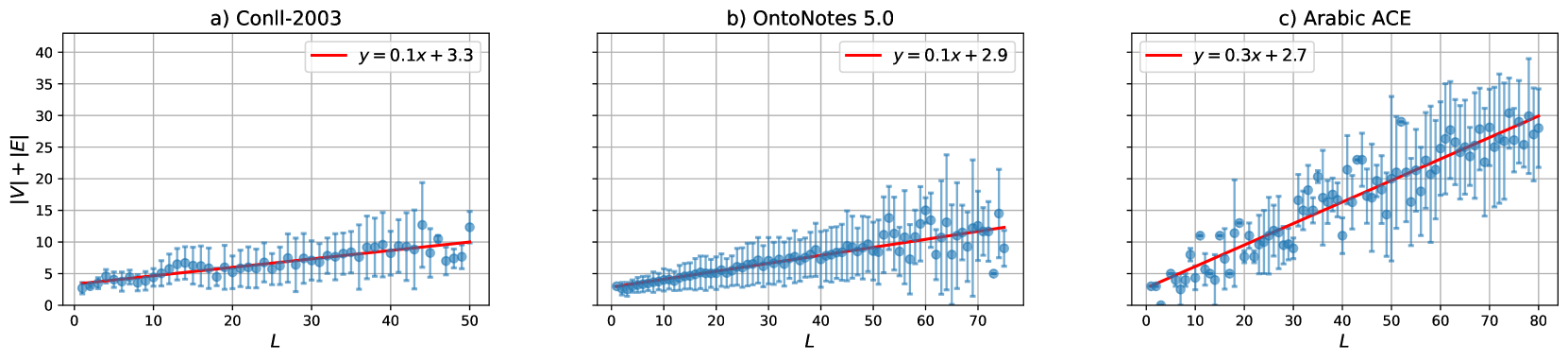
Figure 2: Empirical complexity analysis. We conducted an empirical complexity analysis using trained Filtered Semi-CRF models. The plot showcases the relationship between the size of the filtered graph ($|V|+|E|$) and the input sequence length $L$ on three NER datasets. As the length of the input sequence increases, the graph size seems to grow in a linear fashion.

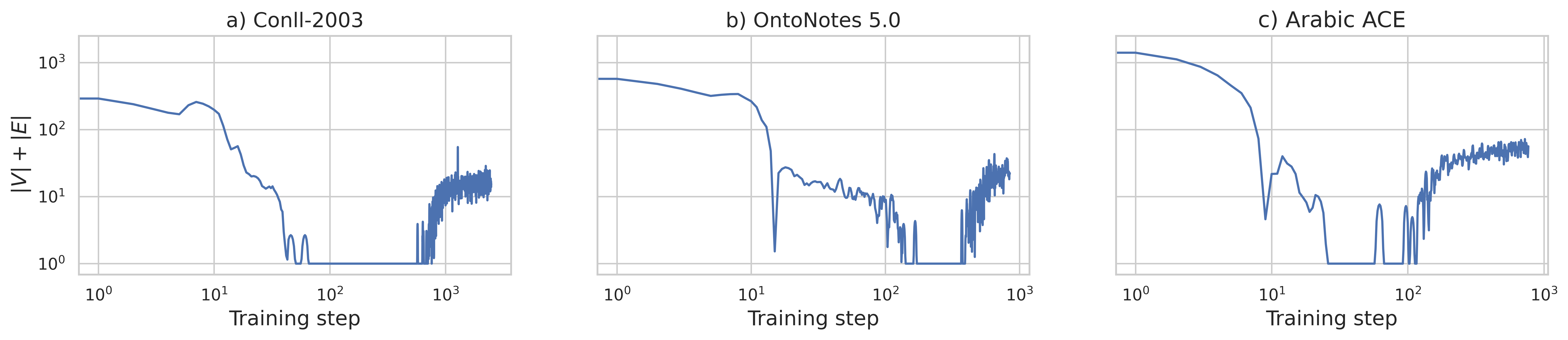
Figure 3: Graph Size during Training. The graph size ($|V|+|E|+1$) undergoes three stages during training: 1) initially large when the filtering classifier is untrained, 2) decreasing in the second stage as most of segments in the training set have a null label (biasing the classifier toward this label), and 3) increasing again as the classifier improves, better aligning with the training dataset statistics.

4.4 Complexity analysis

In this section, we analyze the complexity of the algorithms 1 and 2, $\mathcal{O}(|V|+|E|)$, as a function of the input sequence length $L$. Note that the size of $V$ does not depend on the number of labels $|Y|$ since there is at most one label per segment due to the filtering step in equation 10.

Proposition 4.1.

The number of nodes in a Semi-CRF graph (as described in § 2.4) with an input length of $L$ is given by $\frac{L(L+1)}{2}$.

Proposition 4.2.

The number of edges in a Semi-CRF graph (as described in § 2.4) with an input length of $L$ is given by $\frac{L(L-1)(L+1)}{6}$.

We employ these propositions to determine the complexity of the Filtered Semi-CRF model in the following. The proofs for these propositions can be found in Appendix § A.1.

Worst case complexity

In the worst case scenario, the filtering model $\bm{\phi}_{local}$ does not filter any segments, resulting in all segments being retained. By utilizing Propositions 3.1 and 3.2, we can deduce that in the worst case, $\mathcal{O}(|V|)=\mathcal{O}(L^{2})$ and $\mathcal{O}(|E|)=\mathcal{O}(L^{3})$. This implies that the complexity of our algorithm in the worst case is cubic with respect to the sequence length $L$, as $\mathcal{O}(|V|+|E|)=\mathcal{O}(L^{3})$. However, it is worth noting that in this worst case scenario, the resulting graph is the Semi-CRF and the complexity can be reduced to $L^{2}$ by utilizing the Forward algorithm during training and the Viterbi algorithm during inference (Eq. 19 and Eq. 18).

Best Case Complexity

In the ideal scenario, the filtering process is optimal, resulting in the number of nodes in the graph $|V|$ being equal to the true number of non-null segments in the input sequence, denoted by $\mathcal{S}$. Furthermore, since $\mathcal{S}$ does not contain overlapping segments, $|\mathcal{S}|\leq L$ with $|\mathcal{S}|=L$ if all segments in $\mathcal{S}$ have unit length and cover the entire sequence, i.e., $\mathcal{S}=\{(i,i,l_{i})|i=1\ldots L,l_{i}\neq\texttt{null}\}$. Additionally, $|E|=|\mathcal{S}|-1\leq L-1$ as optimal filtering implies that the path number is unique. As a result, in this best case scenario, the complexity of the algorithm is linear with respect to the sequence length $L$, i.e., $\mathcal{O}(L)$.

Empirical Analysis

In this study, we assess our model’s empirical complexity by examining the correlation between the graph size ($|V|+|E|$) and the input sequence length $L$. We use three popular NER datasets for this analysis - CoNLL-2003, OntoNotes 5.0, and Arabic ACE. Our findings (shown in Figure 2) indicate a linear increase in the graph size as the sequence length increases. Interestingly, the graph size always stays smaller than the sequence length. This suggests that in practice, the computational complexity of the FSemiCRF model is at worst, $\mathcal{O}(L)$. However, during the initial stages of model training, the graph size may be large because the filtering model, which is responsible for reducing the graph size, is not fully trained, as depicted in Figure 3. But, the graph size decreases rapidly after a few training steps as the filtering classifier is improving.

Models	CoNLL-2003			OntoNotes 5.0			Arabic ACE
	P	R	F	P	R	F	P	R	F
Yu et al. (2020)	93.7	93.3	93.5	91.1	91.5	91.3	-	-	-
Yan et al. (2021)	92.61	93.87	93.24	89.99	90.77	90.38	-	-	-
Zhu and Li (2022)	93.61	93.68	93.65	91.75	91.74	91.74	-	-	-
Shen et al. (2022)	93.29	92.46	92.87	91.43	90.73	90.96	-	-	-
Zaratiana et al. (2022a)	94.29	93.33	93.81	90.21	91.21	90.71	85.35	83.64	84.49
El Khbir et al. (2022)	-	-	-	-	-	-	84.42	84.05	84.23
Our experiments
CRF	93.29	92.21	92.75	89.00	90.16	89.57	82.79	84.44	83.61
Semi-CRF	92.37	90.49	91.42	88.91	89.78	89.34	82.97	84.24	83.60
+ Unit size null†	92.08	91.41	91.74	89.17	89.76	89.47	83.35	83.62	83.48
FSemiCRF	94.72	93.09	93.89	90.69	91.31	91.00	83.43	85.51	84.46
– w/o $\mathcal{L}_{\textit{global}}$ (14)†	94.24	92.70	93.46	90.85	89.57	90.21	83.73	83.56	83.64

Table 1: Main Results. All English models employ bert-large-cased as token representations for English datasets, except (Yan et al., 2021) that uses bart-large. ^† See the ablation study (§ 7) for details.

5 Experimental setups

Datasets and evaluation

We evaluate our models on on three diverse Named Entity Recognition (NER) datasets: CoNLL-2003 and OntoNotes 5.0, both English, and Arabic ACE (further details in Appendix A.4). We adopt the standard NER evaluation methodology, calculating precision (P), recall (R), and F1-score (F), based on the exact match between predicted and actual entities.

Hyperparameters

To produce contextual token representations, we used bert-large-cased (Devlin et al., 2019) for both CoNLL-2003 and OntoNotes 5.0 datasets, and bert-base-arabertv2 (Antoun et al., 2020) for Arabic ACE. For simplicity, we do not use auxiliary embeddings (eg. character embeddings). All models are trained with Adam optimizer (Kingma and Ba, 2015). We employed a learning rate of 2e-5 for the pre-trained parameters and a learning rate of 5e-4 for the other parameters. We used a batch size of 8 and trained for a maximal epoch of 15. We keep the best model on the validation set for testing. In this work, for all segment-based model, we restrict the segment to a maximum width $K$ to reduce complexity without harming the recall score on the training set (however some segments may be missed for the test set). By bounding the maximum width of the segments, we reduce the number of segments from $L^{2}$ to $LK$. Under this setup, the complexity of the Semi-Markov CRF becomes $O(LK|Y|^{2})$. We implemented our model with PyTorch (Paszke et al., 2019). The pre-trained transformer models were loaded from HuggingFace’s Transformers library, we used AllenNLP (Gardner et al., 2018) for data preprocessing and the seqeval library (Nakayama, 2018) for evaluating the sequence labeling models. Our Semi-CRF implementation is based on pytorch-struct (Rush, 2020). We trained all the models on a server with V100 GPUs.

Baselines

We compare our Filtered Semi-CRF model against the CRF (Lafferty et al., 2001) and Semi-CRF (Sarawagi and Cohen, 2005). Additionally, we include results from previous studies: BiaffineNER (Yu et al., 2020), BartNER (Yan et al., 2021), Boundary Smoothing (Zhu and Li, 2022), PIQN (Shen et al., 2022), GSS (Zaratiana et al., 2022a) and ArabIE El Khbir et al. (2022). For English datasets, models use bert-large-case (except BartNER with bart-large). Our model for Arabic data utilizes bert-base-arabertv2.

6 Main results

FSemiCRF vs. CRF and Semi-CRF

As shown in Table 1, our FSemiCRF model outperforms both the CRF and Semi-CRF reference models in all datasets, validating its effectiveness. The Semi-CRF model, while providing competitive results, often lags behind, either matching or slightly underperforming the CRF model. This observation is in line with the findings of Liang (2005).

Comparison to pior works

In our work, we mainly compare our approach with previous work that we consider comparable, i.e. that uses sentence-level context and the same backbone model. As shown in the Table 1, on all datasets, we found that our FSemiCRF achieves competitive results on all the datasets. For example, our approach outperforms a span-based model we proposed earlier Zaratiana et al. (2022a), which uses the Maximum weighted independent set to select the best spans.

	CoNLL-2003 (|Y| = 4)			OntoNotes 5.0 (|Y| = 18)			Arabic ACE (|Y| = 7)
	CRF	Semi-CRF	FSemiCRF	CRF	Semi-CRF	FSemiCRF	CRF	Semi-CRF	FSemiCRF
Scoring	3.9	3.9	3.9	4.8	4.9	4.9	8.1	8.3	8.3
Decoding	2.7	3.7	0.2	4.4	27.5	0.2	6.0	10.1	0.3
Decoding Speedup	1.3x	1.0x	18.5x	6.2x	1.0x	137x	1.7x	1.0x	33.7x
Overall	6.6	7.6	4.1	9.2	32.4	5.1	14.1	18.4	8.6
Overall Speedup	1.1x	1.0x	1.8x	3.5x	1.0x	6.3x	1.30x	1.0x	2.1x

Table 2: Inference Wall Clock Time (lower is better). Comparison of required wall-clock time for the scoring (tokens for CRF, segments for Semi-CRF/FSemiCRF) and decoding processes, measured in milliseconds / sample.

7 Ablation study

Semi-CRF + Unit null

We study a variation of the Semi-CRF that only allows for the use of null labels for unit length segments. To do this, we simply modify the original Semi-CRF by eliminating/masking segmentation paths that contain null segments with a size greater than one. The motivation for this study is to fix the multiple redundant paths problem of the Semi-CRF (§ 3). The results show that this approach improves performance on most of the datasets, but still does not perform as well as the other methods, thus validating the importance of segment filtering.

FSemiCRF w/o global loss

We investigate the impact of removing the global loss (Eq. 14) component on our FSemiCRF model, resulting in a local span classfication model. The results are presented in Table 1 (w/o $\mathcal{L}_{\textit{global}}$), and show that even without the global loss component, the model still performs competitively. However, including global loss consistently improves the overall scores of FSemiCRF across all the datasets.

7.1 Efficiency analysis

This section focuses on the computational efficiency of different models, for both training and inference. For this experiment, all the models use a base size for the encoder to ensure a fair comparison.

Inference wall clock time

The wall clock time analysis for scoring and decoding operations, summarized in Table 2, highlights subtle differences in scoring times across all models. However, when it comes to decoding, FSemiCRF significantly outperforms both CRF and Semi-CRF models on all datasets. Notably, FSemiCRF achieves a remarkable 137x speedup over Semi-CRF on the OntoNotes 5.0. Overall, FSemiCRF demonstrates superior performance, being up to 6x and 2x faster than CRF and Semi-CRF, respectively.

Training throughput

Figure 4 presents the training throughput of the models, which measures the number of batches processed per second using a batch size of 8. It reveals that, in general, CRF is the fastest during training, with FSemiCRF following closely as the second fastest model. This can be attributed to the larger graph size of FSemiCRF during training, particularly in the early stages, which can potentially slow down the process, as discussed in the complexity analysis (4.4). However, the differences in training performance between the models are not as pronounced as during inference.

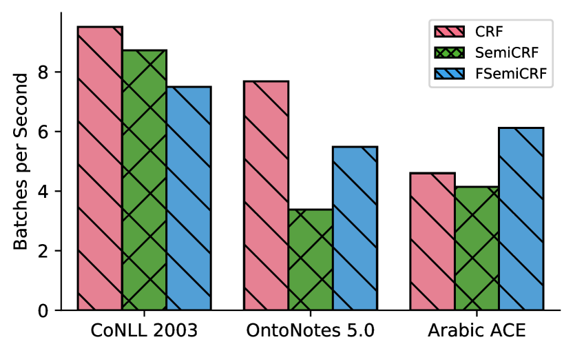
Figure 4: Training throughput in batches per second.

8 Related Work

Linear-chain CRF

Numerous frameworks exist for text segmentation. The commonly used Linear-Chain CRF (Lafferty et al., 2001) treats this task as token-level prediction, training through sequence-level objectives and using the Viterbi algorithm (Viterbi, 1967; Forney, 2010) for decoding. Variants have evolved from using handcrafted features (Lafferty et al., 2001; Gross et al., 2006; Roth and tau Yih, 2005) to automated feature learning through neural networks (Do and Artières, 2010; van der Maaten et al., 2011; Kim et al., 2015; Huang et al., 2015; Lample et al., 2016). Higher order dependencies (Markov order $N>1$) have been explored for enhanced performance, but their adoption is limited due to complexity and marginal gains (Ye et al., 2009; Cuong et al., 2014).

Semi-Markov CRF

Semi-CRF (Sarawagi and Cohen, 2005) is an alternative operating at segment level, applied to tasks like Chinese word segmentation (Kong et al., 2016) and Named Entity Recognition (Sarawagi and Cohen, 2005; Andrew, 2006; Zhuo et al., 2016; Liu et al., 2016a; Ye and Ling, 2018). It has the advantage of incorporating segment-level features but suffers from quadratic complexity and generally equivalent or marginally better performance than CRFs (Liang, 2005; Daumé and Marcu, 2005; Andrew, 2006).

Dynamic Programming Pruning

Prior research has investigated the use of pruning techniques in dynamic programming to improve the efficiency of structured prediction tasks (Roark and Hollingshead, 2008; Rush and Petrov, 2012; Bodenstab et al., 2011; Vieira and Eisner, 2017). These approaches aim to optimize runtime by selectively discarding hypotheses during inference. However, these methods often involve a trade-off between efficiency and performance. In contrast, our Filtered Semi-CRF model introduces a learned filtering step that collaboratively improves both efficiency and overall model performance.

Named Entity Recognition

NER is an important task in Natural Language Processing and is used in many downstream information extraction applications such as relation extraction (Zaratiana et al., 2023) and taxonomy construction (Zhang et al., 2018; Dauxais et al., 2022). Usually, NER tasks are designed as sequence labelling (Huang et al., 2015; Lample et al., 2016; Akbik et al., 2018) where the goal is to predict tagged sequence (eg. BIO tags). Recently, different approaches have been proposed to perform NER tasks that go beyond traditional sequence labelling. One approach that has been widely adopted is the span-based approach (Liu et al., 2016b; Fu et al., 2021; Li et al., 2021; Zaratiana et al., 2022a, b, c; Lou et al., 2022; Corro, 2023) where the prediction is done in the span level instead of entity level. Futhermore, the use of the sequence-to sequence models for Named Entity Recognition has become popular recently. For instance, Yan et al. (2021) uses the BART (Lewis et al., 2019) model to generate named entity using encoder-decoder with copy mechanism.

9 Conclusion

In this paper, we introduce Filtered Semi-CRF, a novel algorithm for text segmentation tasks. By applying our method to NER, we show substantial performance gains over traditional CRF and Semi-CRF models on several datasets. Additionally, our algorithm exhibits improved efficiency, speed, and scalability compared to the baselines. As future work, we plan to investigate the extension of Filtered Semi-CRF to nested segment structures.

Limitations

While our Filtered Semi-CRF model offers several advantages, it also has limitations that should be considered:

Sensitivity to Filtering Quality

The overall performance and efficiency heavily rely on the accuracy of the filtering process in identifying high-quality candidate segments. Inaccurate filtering or the introduction of errors during this step can adversely affect the model’s performance.

Restriction to Non-overlapping Entities

Our model is designed specifically for non-overlapping entity segmentation. It assumes that entities within the text do not overlap with each other. While this assumption is valid for many applications and datasets, scenarios exist where specific cases of entity overlap occurs, such as nested entities.

Appendix A Appendix

A.1 Proofs

Proposition 3.1

The number of nodes in a Semi-CRF graph (as described in § 2.4) with an input length of $L$ is given by $\frac{L(L+1)}{2}$.

Proof.

Nodes are the enumeration of all segments (regardless of labels). Thus,

$$V=\bigcup_{i=1}^{L}\bigcup_{j=i}^{L}(i,j)\Longrightarrow|V| =\sum_{i=1}^{L}\sum_{j=i}^{L}1=\sum_{i=1}^{L}(L+1-i)$$

$$=\sum_{i=1}^{L}(L+1)-\sum_{i=1}^{L}i=L(L+1)-\frac{L(L+1)}{2}$$ (15)

$$|V| =\frac{L(L+1)}{2}$$

∎

Proposition 3.2

The number of edges in a Semi-CRF graph (as described in § 2.4) with an input length of $L$ is given by $\frac{L(L-1)(L+1)}{6}$.

Proof.

We know that in the complete segment graph

1. By definition, $(i_{k},j_{k})\rightarrow(i_{k^{\prime}},j_{k^{\prime}})\in E$ iff $j_{k}+1=i_{k^{\prime}}$

2. There are $j_{k}$ segments ending at $j_{k}$ i.e $|\bigcup_{i=1}^{j_{k}}(i,j_{k})|={\color[rgb]{0,0,1}j_{k}}$

3. There are $L-j_{k}$ segments starting at $i_{k^{\prime}}$ i.e $|\bigcup_{i=i_{k^{\prime}}}^{L}(i_{k^{\prime}},i)|=L-i_{k^{\prime}}+1={\color[rgb]{1,0,0}L-j_{k}}$

From 1, 2 and 3, we can deduce that there is ${\color[rgb]{0,0,1}j_{k}}({\color[rgb]{1,0,0}L-j_{k}})$ segments starting at $i_{k^{\prime}}$ and ending at $j_{k}$. Finally, the total number of edges of the graph is the sum over all $j_{k}$ from $0$ to $L$:

$$|E| =\sum_{j_{k}=1}^{L}{\color[rgb]{0,0,1}j_{k}}({\color[rgb]{1,0,0}L-j_{k}})=L\sum_{j_{k}=1}^{L}j_{k}-\sum_{j_{k}=1}^{L}j_{k}^{2}$$

$$=L\frac{L(L+1)}{2}-\frac{L(L+1)(2L+1)}{6}=L(L+1)(\frac{L}{2}-\frac{2L+1}{6})$$ (16)

$$|E| =\frac{L(L+1)(L-1)}{6}$$

∎

A.2 CRF

Partition function

The partition function $\mathcal{Z}({\bm{x}})$ of the CRF (Lafferty et al., 2001) is computed using the forward algorithm, with $\alpha(1,y)=\bm{\psi}(y|{\bm{x}})$ and for $i=2\ldots L$:

$$\begin{split}\alpha(i,y)=\sum_{y^{\prime}\in Y}\alpha(i-1,y^{\prime})\exp\{\bm{\psi}(y|{\bm{x}})+{\bm{T}}[y^{\prime},y]\}\\ \mathcal{Z}({\bm{x}})=\sum_{y\in Y}\alpha(L,y)\end{split}$$ (17)

Decoding

The decoding of CRF is done with the Viterbi algorithm, with $\delta(1,y)=\bm{\psi}(y|{\bm{x}})$

$$\delta(i,y)=\max_{y^{\prime}\in Y}\delta(i-1,y^{\prime})+\bm{\psi}(y|{\bm{x}})+{\bm{T}}[y^{\prime},y]$$ (18)

The best labeling is given by the path traced by $\max_{y\in Y}\delta(L,y)$. Both the computation of the partition function and the decoding of the CRF have a complexity of $\mathcal{O}(L|Y|^{2})$.

A.3 Semi-CRF

Partition function

The partition function of the Semi-CRF (Sarawagi and Cohen, 2005) $\mathcal{Z}({\bm{x}})$ is computed using the following dynamic program (a modification of the forward algorithm) with $\alpha(0,:)=1$ and $\alpha(m,:)=0$ if $m<0$ and otherwise:

$$\begin{split}\alpha(m,y)=\sum_{d=1}^{L}\sum_{y^{\prime}\in Y}\alpha(m-d,y^{\prime})\exp\left\{\bm{\phi}((i=m-d+1,j=m,l=y)|{\bm{x}})+{\bm{T}}[y^{\prime},y]\right\}\\ \mathcal{Z}({\bm{x}})=\sum_{y\in Y}\alpha(L,y)\end{split}$$ (19)

Decoding

The decoding of the Semi-CRF is done with the segmental/Semi-Markov Viterbi algorithm with $\delta(0,:)=0$ and $\delta(m,:)=-\infty$ if $m<0$ and otherwise:

$$\delta(m,y)=\max_{\begin{subarray}{c}y^{\prime}\in Y\\ d=1\ldots L\end{subarray}}\delta(i-d,y^{\prime})+\bm{\phi}((i=m-d+1,j=m,l=y)|{\bm{x}})+{\bm{T}}[y^{\prime},y]$$ (20)

The highest scoring segmentation is the path traced by $\max_{y\in Y}\delta(L,y)$. Both the computation of the partition function and the decoding of the Semi-CRF have a complexity of $\mathcal{O}(L^{2}|Y|^{2})$.

A.4 Datasets

We evaluate our models on three diverse datasets of Named Entity Recognition. CoNLL-2003 (Tjong Kim Sang and De Meulder, 2003) is a dataset from the news domain designed for extracting entities such as Person, Location, and Organization. OntoNotes 5.0 (Weischedel et al., 2013) is a large corpus comprising various kinds of text, including newswire, broadcast news, and telephone conversation, with a total of 18 different entity types, such as Person, Organization, Location, Product, or Date. Arabic ACE is the Arabic portion of the multilingual information extraction corpus, ACE 2005 (Walker et al., 2006). It includes texts from a wide range of genres, such as newswire, broadcast news, and weblogs, with a total of 7 entity types.

References

- Akbik et al. (2018) Alan Akbik, Duncan Blythe, and Roland Vollgraf. 2018. Contextual string embeddings for sequence labeling. In Proceedings of the 27th International Conference on Computational Linguistics, pages 1638–1649, Santa Fe, New Mexico, USA. Association for Computational Linguistics.
- Andrew (2006) Galen Andrew. 2006. A hybrid Markov/semi-Markov conditional random field for sequence segmentation. In Proceedings of the 2006 Conference on Empirical Methods in Natural Language Processing, pages 465–472, Sydney, Australia. Association for Computational Linguistics.
- Antoun et al. (2020) Wissam Antoun, Fady Baly, and Hazem Hajj. 2020. AraBERT: Transformer-based model for Arabic language understanding. In Proceedings of the 4th Workshop on Open-Source Arabic Corpora and Processing Tools, with a Shared Task on Offensive Language Detection, pages 9–15, Marseille, France. European Language Resource Association.
- Bodenstab et al. (2011) Nathan Bodenstab, Aaron Dunlop, Keith Hall, and Brian Roark. 2011. Beam-width prediction for efficient context-free parsing. In Proceedings of the 49th Annual Meeting of the Association for Computational Linguistics: Human Language Technologies, pages 440–449, Portland, Oregon, USA. Association for Computational Linguistics.
- Corro (2023) Caio Corro. 2023. A dynamic programming algorithm for span-based nested named-entity recognition in . In Proceedings of the 61st Annual Meeting of the Association for Computational Linguistics (Volume 1: Long Papers), pages 10712–10724, Toronto, Canada. Association for Computational Linguistics.
- Cuong et al. (2014) Nguyen Viet Cuong, Nan Ye, Wee Sun Lee, and Hai Leong Chieu. 2014. Conditional random field with high-order dependencies for sequence labeling and segmentation. Journal of Machine Learning Research, 15(28):981–1009.
- Daumé and Marcu (2005) Hal Daumé and Daniel Marcu. 2005. Learning as search optimization: approximate large margin methods for structured prediction. Proceedings of the 22nd international conference on Machine learning.
- Dauxais et al. (2022) Yann Dauxais, Urchade Zaratiana, Matthieu Laneuville, Simon David Hernandez, Pierre Holat, and Charlie Grosman. 2022. Towards automation of topic taxonomy construction. In Advances in Intelligent Data Analysis XX: 20th International Symposium on Intelligent Data Analysis, IDA 2022, Rennes, France, April 20–22, 2022, Proceedings, page 26–38, Berlin, Heidelberg. Springer-Verlag.
- Devlin et al. (2019) Jacob Devlin, Ming-Wei Chang, Kenton Lee, and Kristina Toutanova. 2019. BERT: Pre-training of deep bidirectional transformers for language understanding. In Proceedings of the 2019 Conference of the North American Chapter of the Association for Computational Linguistics: Human Language Technologies, Volume 1 (Long and Short Papers), pages 4171–4186, Minneapolis, Minnesota. Association for Computational Linguistics.
- Do and Artières (2010) Trinh Minh Tri Do and Thierry Artières. 2010. Neural conditional random fields. In AISTATS.
- El Khbir et al. (2022) Niama El Khbir, Nadi Tomeh, and Thierry Charnois. 2022. ArabIE: Joint entity, relation and event extraction for Arabic. In Proceedings of the The Seventh Arabic Natural Language Processing Workshop (WANLP), pages 331–345, Abu Dhabi, United Arab Emirates (Hybrid). Association for Computational Linguistics.
- Forney (2010) Jr. G. Forney. 2010. Viterbi algorithm. In Encyclopedia of Machine Learning.
- Fu et al. (2021) Jinlan Fu, Xuanjing Huang, and Pengfei Liu. 2021. SpanNER: Named entity re-/recognition as span prediction. In Proceedings of the 59th Annual Meeting of the Association for Computational Linguistics and the 11th International Joint Conference on Natural Language Processing (Volume 1: Long Papers), pages 7183–7195, Online. Association for Computational Linguistics.
- Gardner et al. (2018) Matt Gardner, Joel Grus, Mark Neumann, Oyvind Tafjord, Pradeep Dasigi, Nelson F. Liu, Matthew Peters, Michael Schmitz, and Luke Zettlemoyer. 2018. AllenNLP: A deep semantic natural language processing platform. In Proceedings of Workshop for NLP Open Source Software (NLP-OSS), pages 1–6, Melbourne, Australia. Association for Computational Linguistics.
- Gross et al. (2006) Samuel Gross, Olga Russakovsky, Chuong B., and Serafim Batzoglou. 2006. Training conditional random fields for maximum labelwise accuracy. In Advances in Neural Information Processing Systems, volume 19. MIT Press.
- Huang et al. (2015) Zhiheng Huang, Wei Xu, and Kai Yu. 2015. Bidirectional lstm-crf models for sequence tagging.
- Kim et al. (2015) Young-Bum Kim, Karl Stratos, and Ruhi Sarikaya. 2015. Pre-training of hidden-unit CRFs. In Proceedings of the 53rd Annual Meeting of the Association for Computational Linguistics and the 7th International Joint Conference on Natural Language Processing (Volume 2: Short Papers), pages 192–198, Beijing, China. Association for Computational Linguistics.
- Kingma and Ba (2015) Diederik P. Kingma and Jimmy Ba. 2015. Adam: A method for stochastic optimization. In 3rd International Conference on Learning Representations, ICLR 2015, San Diego, CA, USA, May 7-9, 2015, Conference Track Proceedings.
- Kong et al. (2016) Lingpeng Kong, Chris Dyer, and Noah A. Smith. 2016. Segmental recurrent neural networks. CoRR, abs/1511.06018.
- Lafferty et al. (2001) John D. Lafferty, Andrew McCallum, and Fernando C. N. Pereira. 2001. Conditional random fields: Probabilistic models for segmenting and labeling sequence data. In Proceedings of the Eighteenth International Conference on Machine Learning, ICML ’01, page 282–289, San Francisco, CA, USA. Morgan Kaufmann Publishers Inc.
- Lample et al. (2016) Guillaume Lample, Miguel Ballesteros, Sandeep Subramanian, Kazuya Kawakami, and Chris Dyer. 2016. Neural architectures for named entity recognition. In North American Chapter of the Association for Computational Linguistics.
- Lewis et al. (2019) Mike Lewis, Yinhan Liu, Naman Goyal, Marjan Ghazvininejad, Abdelrahman Mohamed, Omer Levy, Ves Stoyanov, and Luke Zettlemoyer. 2019. Bart: Denoising sequence-to-sequence pre-training for natural language generation, translation, and comprehension.
- Li and Yuan (1998) Haizhou Li and Baosheng Yuan. 1998. Chinese word segmentation. In Proceedings of the 12th Pacific Asia Conference on Language, Information and Computation, pages 212–217, Singapore. Chinese and Oriental Languages Information Processing Society.
- Li et al. (2021) Yangming Li, lemao liu, and Shuming Shi. 2021. Empirical analysis of unlabeled entity problem in named entity recognition. In International Conference on Learning Representations.
- Liang (2005) Percy Liang. 2005. Semi-supervised learning for natural language.
- Liang et al. (1991) Y.D. Liang, S.K. Dhall, and S. Lakshmivarahan. 1991. On the problem of finding all maximum weight independent sets in interval and circular-arc graphs. In [Proceedings] 1991 Symposium on Applied Computing, pages 465–470.
- Liu et al. (2016a) Yijia Liu, Wanxiang Che, Jiang Guo, Bing Qin, and Ting Liu. 2016a. Exploring segment representations for neural segmentation models. In IJCAI.
- Liu et al. (2016b) Yijia Liu, Wanxiang Che, Jiang Guo, Bing Qin, and Ting Liu. 2016b. Exploring segment representations for neural segmentation models. In Proceedings of the Twenty-Fifth International Joint Conference on Artificial Intelligence, IJCAI’16, page 2880–2886. AAAI Press.
- Lou et al. (2022) Chao Lou, Songlin Yang, and Kewei Tu. 2022. Nested named entity recognition as latent lexicalized constituency parsing. In Proceedings of the 60th Annual Meeting of the Association for Computational Linguistics (Volume 1: Long Papers), pages 6183–6198, Dublin, Ireland. Association for Computational Linguistics.
- Nakayama (2018) Hiroki Nakayama. 2018. seqeval: A python framework for sequence labeling evaluation. Software available from https://github.com/chakki-works/seqeval.
- Paszke et al. (2019) Adam Paszke, Sam Gross, Francisco Massa, Adam Lerer, James Bradbury, Gregory Chanan, Trevor Killeen, Zeming Lin, Natalia Gimelshein, Luca Antiga, Alban Desmaison, Andreas Kopf, Edward Yang, Zachary DeVito, Martin Raison, Alykhan Tejani, Sasank Chilamkurthy, Benoit Steiner, Lu Fang, Junjie Bai, and Soumith Chintala. 2019. Pytorch: An imperative style, high-performance deep learning library. In H. Wallach, H. Larochelle, A. Beygelzimer, F. d'Alché-Buc, E. Fox, and R. Garnett, editors, Advances in Neural Information Processing Systems 32, pages 8024–8035.
- Rabiner (1989) L.R. Rabiner. 1989. A tutorial on hidden markov models and selected applications in speech recognition. Proceedings of the IEEE, 77(2):257–286.
- Ratinov and Roth (2009) Lev Ratinov and Dan Roth. 2009. Design challenges and misconceptions in named entity recognition. In Proceedings of the Thirteenth Conference on Computational Natural Language Learning (CoNLL-2009), pages 147–155, Boulder, Colorado. Association for Computational Linguistics.
- Roark and Hollingshead (2008) Brian Roark and Kristy Hollingshead. 2008. Classifying chart cells for quadratic complexity context-free inference. In Proceedings of the 22nd International Conference on Computational Linguistics (Coling 2008), pages 745–752, Manchester, UK. Coling 2008 Organizing Committee.
- Roth and tau Yih (2005) Dan Roth and Wen tau Yih. 2005. Integer linear programming inference for conditional random fields. Proceedings of the 22nd international conference on Machine learning.
- Rush (2020) Alexander Rush. 2020. Torch-struct: Deep structured prediction library. In Proceedings of the 58th Annual Meeting of the Association for Computational Linguistics: System Demonstrations, pages 335–342, Online. Association for Computational Linguistics.
- Rush and Petrov (2012) Alexander Rush and Slav Petrov. 2012. Vine pruning for efficient multi-pass dependency parsing. In The 2012 Conference of the North American Chapter of the Association for Computational Linguistics: Human Language Technologies (NAACL ’12), page Best Paper Award.
- Sarawagi and Cohen (2005) Sunita Sarawagi and William W Cohen. 2005. Semi-markov conditional random fields for information extraction. In Advances in Neural Information Processing Systems, volume 17. MIT Press.
- Shen et al. (2022) Yongliang Shen, Xiaobin Wang, Zeqi Tan, Guangwei Xu, Pengjun Xie, Fei Huang, Weiming Lu, and Yue Ting Zhuang. 2022. Parallel instance query network for named entity recognition. In ACL.
- Tjong Kim Sang and De Meulder (2003) Erik F. Tjong Kim Sang and Fien De Meulder. 2003. Introduction to the CoNLL-2003 shared task: Language-independent named entity recognition. In Proceedings of the Seventh Conference on Natural Language Learning at HLT-NAACL 2003, pages 142–147.
- van der Maaten et al. (2011) Laurens van der Maaten, Max Welling, and Lawrence K. Saul. 2011. Hidden-unit conditional random fields. In AISTATS.
- Vieira and Eisner (2017) Tim Vieira and Jason Eisner. 2017. Learning to prune: Exploring the frontier of fast and accurate parsing. Transactions of the Association for Computational Linguistics, 5:263–278.
- Viterbi (1967) A. Viterbi. 1967. Error bounds for convolutional codes and an asymptotically optimum decoding algorithm. IEEE Transactions on Information Theory, 13(2):260–269.
- Wainwright and Jordan (2008) Martin J. Wainwright and Michael I. Jordan. 2008. Graphical models, exponential families, and variational inference. Foundations and Trends® in Machine Learning, 1(1–2):1–305.
- Walker et al. (2006) Christopher Walker, Stephanie Strassel, Julie Medero, and Kazuaki Maeda. 2006. Ace 2005 multilingual training corpus.
- Weischedel et al. (2013) Ralph Weischedel, Martha Palmer, Mitchell Marcus, Eduard Hovy, Sameer Pradhan, Lance Ramshaw, Nianwen Xue, Ann Taylor, Jeff Kaufman, Michelle Franchini, Mohammed El-Bachouti, Robert Belvin, and Ann Houston. 2013. OntoNotes Release 5.0.
- Yan et al. (2021) Hang Yan, Tao Gui, Junqi Dai, Qipeng Guo, Zheng Zhang, and Xipeng Qiu. 2021. A unified generative framework for various NER subtasks. In Proceedings of the 59th Annual Meeting of the Association for Computational Linguistics and the 11th International Joint Conference on Natural Language Processing (Volume 1: Long Papers), pages 5808–5822, Online. Association for Computational Linguistics.
- Ye et al. (2009) Nan Ye, Wee Lee, Hai Chieu, and Dan Wu. 2009. Conditional random fields with high-order features for sequence labeling. In Advances in Neural Information Processing Systems, volume 22. Curran Associates, Inc.
- Ye and Ling (2018) Zhixiu Ye and Zhen-Hua Ling. 2018. Hybrid semi-Markov CRF for neural sequence labeling. In Proceedings of the 56th Annual Meeting of the Association for Computational Linguistics (Volume 2: Short Papers), pages 235–240, Melbourne, Australia. Association for Computational Linguistics.
- Yu et al. (2020) Juntao Yu, Bernd Bohnet, and Massimo Poesio. 2020. Named entity recognition as dependency parsing. In Proceedings of the 58th Annual Meeting of the Association for Computational Linguistics, pages 6470–6476, Online. Association for Computational Linguistics.
- Zaratiana et al. (2022a) Urchade Zaratiana, Niama Elkhbir, Pierre Holat, Nadi Tomeh, and Thierry Charnois. 2022a. Global span selection for named entity recognition. In Proceedings of the Workshop on Unimodal and Multimodal Induction of Linguistic Structures (UM-IoS), pages 11–17, Abu Dhabi, United Arab Emirates (Hybrid). Association for Computational Linguistics.
- Zaratiana et al. (2022b) Urchade Zaratiana, Nadi Tomeh, Pierre Holat, and Thierry Charnois. 2022b. GNNer: Reducing overlapping in span-based NER using graph neural networks. In Proceedings of the 60th Annual Meeting of the Association for Computational Linguistics: Student Research Workshop, pages 97–103, Dublin, Ireland. Association for Computational Linguistics.
- Zaratiana et al. (2022c) Urchade Zaratiana, Nadi Tomeh, Pierre Holat, and Thierry Charnois. 2022c. Named entity recognition as structured span prediction. In Proceedings of the Workshop on Unimodal and Multimodal Induction of Linguistic Structures (UM-IoS), pages 1–10, Abu Dhabi, United Arab Emirates (Hybrid). Association for Computational Linguistics.
- Zaratiana et al. (2023) Urchade Zaratiana, Nadi Tomeh, Pierre Holat, and Thierry Charnois. 2023. An autoregressive text-to-graph framework for joint entity and relation extraction. In ICML 2023 Workshop on Structured Probabilistic Inference & Generative Modeling.
- Zhang et al. (2018) Chao Zhang, Fangbo Tao, Xiusi Chen, Jiaming Shen, Meng Jiang, Brian Sadler, Michelle Vanni, and Jiawei Han. 2018. Taxogen: Unsupervised topic taxonomy construction by adaptive term embedding and clustering. In Proceedings of the 24th ACM SIGKDD International Conference on Knowledge Discovery & Data Mining, KDD ’18, page 2701–2709, New York, NY, USA. Association for Computing Machinery.
- Zhu and Li (2022) Enwei Zhu and Jinpeng Li. 2022. Boundary smoothing for named entity recognition. In Proceedings of the 60th Annual Meeting of the Association for Computational Linguistics (Volume 1: Long Papers), pages 7096–7108, Dublin, Ireland. Association for Computational Linguistics.
- Zhuo et al. (2016) Jingwei Zhuo, Yong Cao, Jun Zhu, Bo Zhang, and Zaiqing Nie. 2016. Segment-level sequence modeling using gated recursive semi-Markov conditional random fields. In Proceedings of the 54th Annual Meeting of the Association for Computational Linguistics (Volume 1: Long Papers), pages 1413–1423, Berlin, Germany. Association for Computational Linguistics.