Subsystem CSS codes, a tighter stabilizer-to-CSS mapping, and Goursat’s Lemma

Abstract

The CSS code construction is a powerful framework used to express features of a quantum code in terms of a pair of underlying classical codes. Its subsystem extension allows for similar expressions, but the general case has not been fully explored. Extending previous work of Aly et. al. [quant-ph/0610153], we determine subsystem CSS code parameters, express codewords, and develop a Steane-type decoder using only data from the two underlying classical codes. We show that any subsystem stabilizer code can be “doubled” to yield a subsystem CSS code with twice the number of physical, logical, and gauge qudits and up to twice the code distance. This mapping preserves locality and is tighter than the Majorana-based mapping of Bravyi, Leemhuis, and Terhal [New J. Phys. 12 083039 (2010)]. Using Goursat’s Lemma, we show that every subsystem stabilizer code can be constructed from two nested subsystem CSS codes satisfying certain constraints, and we characterize subsystem stabilizer codes based on the nested codes’ properties.

I Introduction and summary of results

An extensive theory of quantum error-correcting codes has been developed to protect quantum computers from noise [1, 2, 3] . Qualitatively, a quantum error-correcting code describes how to “hide” quantum information within a protected subsystem of a quantum system, such that noise within the quantum system can be detected and removed from the protected subsystem. The class of quantum error-correcting codes called stabilizer codes [4, 5] remains the most promising route to a working and robust quantum computer, in part due to extra structure that is useful for promptly detecting and correcting errors.

We are interested in the special class of subsystem stabilizer codes [6, 7] , which correspond to the nontrivial normal subgroups of a Pauli group. While subsystem stabilizer codes can be derived from subspace stabilizer codes by using only a subset of the original logical qudits to store quantum information, such codes can exhibit advantageous and/or inherently different properties from subspace stabilizer codes such as lower weights of check operators [8], new fault-tolerant protocols [9], the association with more general types of anyon theories in two dimensions [10], as well as single-shot error correction in three dimensions [11, 12]. The extra data used to define subsystem stabilizer codes yields a richer code structure, warranting its own investigation.

A large part of our work studies subsystem CSS codes [13, 14] , where the corresponding normal subgroup admits a generating set consisting of $X$-type and $Z$-type Pauli operators. Subsystem CSS codes generalize subspace CSS codes [15, 16, 17] , of which there are many useful examples [18, 19], recently culminating in the first asymptotically good quantum low-density parity-check codes [20, 21, 22]. Subspace CSS codes have rich connections to classical coding theory [23, 24, 25] and homology theory [26, 27, 28], and they admit a recovery procedure that utilizes classical linear codes to independently correct $X$-type and $Z$-type Pauli errors [15, 29]. Thus, it is interesting to investigate the generalization of subspace CSS codes to the subsystem setting. Indeed, many subsystem stabilizer codes are CSS [30, 31, 32], so a general theory of subsystem CSS codes would apply to a broad class of examples developed to date.

To study subsystem CSS codes, we adopt a linear-algebraic perspective that streamlines previous proofs and distills the essential mathematical ideas [33]. This places subsystem CSS codes on the same footing as subspace CSS codes, allowing us to generalize many important features of subspace CSS codes to the subsystem setting.

Our main tool is the symplectic representation, which allows us to view a subsystem stabilizer code as a subspace of a vector space by considering Pauli groups modulo phase factors. In this representation, the structure and parameters of a subsystem stabilizer code are encoded in a “tower” of subspaces, which can then be manipulated using tools from linear algebra [34, 35, 36] to yield several general results.

Our results include a mapping from subsystem stabilizer codes to subsystem CSS codes, a fleshing out of the connection between subsystem CSS codes and classical coding theory, a general recovery procedure for subsystem CSS codes, and a characterization of subsystem stabilizer codes based on Goursat’s Lemma from group theory.

In Section II, we review the theory of Pauli groups and subsystem stabilizer codes, and we explain how to translate these objects to the linear algebraic framework.

In Section III, we review the subspace CSS construction and its generalization to the subsystem case. While the subspace CSS construction utilizes two classical linear codes [37] under certain constraints, the subsystem CSS construction utilizes two classical linear codes with no constraints. We express the logical and gauge codewords in terms of the two underlying classical linear codes.

In Section IV, we show that the performance of subsystem CSS codes is comparable to that of subsystem stabilizer codes. More precisely, we show that every modular-qudit subsystem stabilizer code can be “doubled” to yield a subsystem CSS code with twice the number of physical, logical, and gauge qudits and up to twice the code distance.

In Section V, we present an error-correction procedure for subsystem CSS codes that generalizes the well-known Steane procedure for subspace CSS codes (see, e.g., [15, 29, 38]). While specific instances of this procedure have been presented previously [39, 40, 41, 42, 43, 44, 45], we are unaware of a presentation of the general case that uses only information from the underlying classical linear codes. Our error-correction procedure for subsystem CSS codes decodes up to arbitrary actions on the gauge qudits, and the corresponding classical step in our error-correction procedure decodes up to prescribed “redundant” subcodes obtained from the underlying classical codes. We explore an alternative decoder that generalizes the recovery procedure for the Bacon–Shor code [30] in Appendix C.

In Section VI, we show that every subsystem stabilizer code can be constructed from two subsystem CSS codes satisfying certain constraints, much as every subsystem CSS code can be constructed from two classical codes. We investigate the structure of a given subsystem stabilizer code in terms of its two underlying subsystem CSS codes, and we define two code families that can be viewed as generalizations of subsystem CSS codes from this perspective (see Fig. 2).

Finally, we provide concluding remarks in Section VII. Most proofs have been deferred to Appendix A for readability.

II Preliminaries

In Section II.1, we review the construction of Pauli groups. In Section II.2, we explain how to interpret Pauli groups as vector spaces, and we review the related theory of bilinear forms on vector spaces. In Section II.3, we review the construction of subsystem stabilizer codes. Finally, in Section II.4, we explain how to interpret subsystem stabilizer codes as subspaces of vector spaces, and we define the properties of subsystem stabilizer codes in the vector space setting.

II.1 Pauli groups

Consider a quantum system with $n$ prime qudits, each of dimension $p$. The Hilbert space of this system is given by the quantization of $G\coloneqq\mathbb{F}_{p}^{n}$, i.e.,

$$\mathbb{H}\coloneqq\left\langle\{\left|g\right\rangle\mid g\in G\}\right\rangle\cong{\left(\mathbb{C}^{p}\right)}^{\otimes n}.$$ (1)

Acting on this space is a special class of linear operators called Pauli operators, denoted by $X^{a},Z^{b}$ for any $a,b\in G$. For any basis vector $\left|g\right\rangle\in\mathbb{H}$, the Pauli operators act as

$$X^{a}\left|g\right\rangle \coloneqq\left|a+g\right\rangle\text{ and}$$ (2)

$$Z^{b}\left|g\right\rangle \coloneqq e^{\frac{2\pi i}{p}b\cdot g}\left|g\right\rangle,$$ (3)

where $\cdot$ is the usual dot product on $G$. One verifies the relations

$$X^{a}Z^{b}X^{c}Z^{d} =e^{\frac{2\pi i}{p}b\cdot c}X^{a+c}Z^{b+d}\text{ and}$$ (4)

$$X^{a}Z^{b}X^{c}Z^{d} =e^{\frac{2\pi i}{p}(b\cdot c-a\cdot d)}X^{c}Z^{d}X^{a}Z^{b}$$ (5)

among the Pauli operators. We define the weight of a Pauli operator to be the number of qudits on which it acts nontrivially. The Pauli operators generate the Pauli group, which is given explicitly by

$$\mathcal{P} \coloneqq\left\langle\left\{X^{a},Z^{b}\,\middle|\,a,b\in G\right\}\right\rangle$$ (6)

$$=\left\{e^{\frac{2\pi i}{p}\kappa}X^{a}Z^{b}\,\middle|\,\kappa\in\mathbb{F}_{p},a,b\in G\right\}.$$

We remark that in other works, the phase factors included in the Pauli group may differ depending on whether $p$ is odd or even [46, 10, 47]. This will not matter much for our work, since we will henceforth consider Pauli groups modulo phase factors.

II.2 Pauli groups as vector spaces

In light of Eqs. (4) and (6), one sees that the Pauli group modulo phases is essentially equivalent to the vector space $G\times G$. Formally, letting

$$\Phi\coloneqq\left\{e^{\frac{2\pi i}{p}\kappa}\,\middle|\,\kappa\in\mathbb{F}_{p}\right\}$$ (7)

denote the collection of phases in the Pauli group, one verifies that the map

$$\mathcal{P}/\Phi \to G\times G$$ (8)

$$\Phi X^{a}Z^{b} \mapsto(a,b)$$

is a vector space isomorphism. For most of this work, it will be convenient to view the Pauli group modulo phases as the vector space $G\times G$. We review the necessary theory below [33, 34].

A function $\xi:G\times G\to\mathbb{F}_{p}$ is called bilinear if

$$\xi(a+\lambda\,b,c) =\xi(a,c)+\lambda\,\xi(b,c)\text{ and}$$ (9)

$$\xi(a,b+\lambda\,c) =\xi(a,b)+\lambda\,\xi(a,c),$$

symmetric if

$$\xi(a,b)=\xi(b,a),$$ (10)

antisymmetric if

$$\xi(a,b)=-\xi(b,a),$$ (11)

and nondegenerate if

$$\xi(a,G)=0\implies a=0.$$ (12)

We call $\xi$ a form if it is bilinear and nondegenerate. Henceforth, $\xi$ will denote a symmetric or antisymmetric form, $\theta$ will denote a symmetric form, and $\omega$ will denote an antisymmetric form. Every subspace $H\leq G$ has a complement with respect to $\xi$

$$H^{\xi}\coloneqq\left\{a\in G\,\middle|\,\xi(a,H)=0\right\}\leq G.$$ (13)

One verifies that

$$\dim H+\dim H^{\xi} =\dim G\text{ and}$$ (14)

$$\left(H^{\xi}\right)^{\xi} =H.$$ (15)

Moreover, if $K\leq G$ is another subspace, then

$$(H+K)^{\xi} =H^{\xi}\cap K^{\xi}\text{ and}$$ (16)

$$(H\cap K)^{\xi} =H^{\xi}+K^{\xi}.$$ (17)

A symmetric form $\theta$ on $G$ passes naturally to a symmetric form

$$((a,b),(c,d))\mapsto\theta(a,c)+\theta(b,d)$$ (18)

on $G\times G$, which by abuse of notation we also call $\theta$ (note that for the Pauli group, $\theta$ is the dot product). In addition, the original symmetric form $\theta$ on $G$ induces the antisymmetric form

$$\omega((a,b),(c,d))\coloneqq\theta(b,c)-\theta(a,d)$$ (19)

on $G\times G$ (note that for the Pauli group, $\omega$ encodes the commutation of the Pauli operators as in Eq. (5)). Direct products behave well with respect to these induced forms. Indeed, if $H_{X}\times H_{Z}\leq G\times G$, then

$$\left(H_{X}\times H_{Z}\right)^{\theta} =H_{X}^{\theta}\times H_{Z}^{\theta}\text{ and}$$ (20)

$$\left(H_{X}\times H_{Z}\right)^{\omega} =H_{Z}^{\theta}\times H_{X}^{\theta}.$$ (21)

For any $a=(a_{1},\ldots,a_{n}),b=(b_{1},\ldots,b_{n})\in G$, we call

$$\operatorname{wt}(a)\coloneqq\left|\left\{j\in\left\{1,\ldots,n\right\}\mid a_{j}\neq 0\right\}\right|$$ (22)

the weight of $a$, and we call

$$\operatorname{swt}(a,b)\coloneqq\left|\left\{j\in\left\{1,\ldots,n\right\}\mid\left(a_{j},b_{j}\right)\neq(0,0)\right\}\right|$$ (23)

the symplectic weight of $(a,b)$. For any nontrivial $S\subseteq G$ and $T\subseteq G\times G$, we write

$$\min\operatorname{wt}(S) \coloneqq\underset{a\in S\setminus\{0\}}{\min}\operatorname{wt}(a)\text{ and}$$ (24)

$$\min\operatorname{swt}(T) \coloneqq\underset{(a,b)\in T\setminus\{0\}}{\min}\operatorname{swt}(a,b).$$ (25)

Note that the weight of a Pauli operator $X^{a}Z^{b}$ is equal to the symplectic weight of the corresponding vector $(a,b)$.

Finally, for any algebraic objects $G,H$, we write

(26)

to indicate that $H\leq G$ and, if $G,H$ are vector spaces, that $\dim G/H=l$.

II.3 Subsystem stabilizer codes

A subsystem stabilizer code can be interpreted as a subspace stabilizer code with some of its logical qudits relegated to gauge qudits. This necessitates the use of a “gauge group” to determine the gauge qudits.

In the usual formalism for subsystem stabilizer codes [6, 47], one begins with an abelian “stabilizer group” $\mathcal{S}\leq\mathcal{P}$ whose intersection with $\Phi$ is trivial. Then, one considers the centralizer of $\mathcal{S}$, denoted $\mathcal{C}(\mathcal{S})$, which is the subgroup of all Pauli operators that commute with everything in $\mathcal{S}$. Finally, one selects a “gauge group” $\mathcal{G}\leq\mathcal{C}(\mathcal{S})$ whose center is $\left\langle\Phi,\mathcal{S}\right\rangle$. These relationships can be summarized in the tower of normal subgroups

(27)

which encodes the parameters of the subsystem stabilizer code. Indeed, the number of logical (resp. gauge) qudits in $\mathcal{G}$ is given by half the size of any minimal generating set for $\mathcal{C}(\mathcal{S})/\mathcal{G}$ (resp. $\mathcal{G}/{\left\langle\Phi,\mathcal{S}\right\rangle}$). Moreover, the distance of $\mathcal{G}$ is defined to be the minimum weight of a Pauli operator in $\mathcal{C}(\mathcal{S})\setminus\mathcal{G}$.

Observe that every tower as in Eq. (27) determines a gauge group $\Phi\leq\mathcal{G}\leq\mathcal{P}$. Conversely, every gauge group $\Phi\leq\mathcal{G}\leq\mathcal{P}$ determines a tower as in Eq. (27). Thus, in the usual formalism, a subsystem stabilizer code is defined to be a subgroup $\Phi\leq\mathcal{G}\leq\mathcal{P}$. Moreover, one calls $\mathcal{G}$ a subsystem CSS code if $\mathcal{G}$ admits a generating set that consists only of $X$-type or $Z$-type Pauli operators.

Any subsystem stabilizer code $\mathcal{G}$ generates a von Neumann algebra $\operatorname{Alg}\mathcal{G}$ of linear operators on the physical Hilbert space $\mathbb{H}$. This algebra induces an orthogonal decomposition of $\mathbb{H}$ as [6, 47, 48]

$$\mathbb{H}\cong\underset{\tau\mathcal{C}(\mathcal{S})\in\mathcal{P}/\mathcal{C}(\mathcal{S})}{\bigoplus}\tau(\mathbb{L}\otimes\mathbb{G}),$$ (28)

where $\mathbb{L}\otimes\mathbb{G}$ is the subspace of $\mathbb{H}$ fixed by the stabilizer group $\mathcal{S}$. With respect to this decomposition, the algebra $\operatorname{Alg}\mathcal{G}$ takes the form

$$\operatorname{Alg}\mathcal{G}\cong\underset{\tau\mathcal{C}(\mathcal{S})\in\mathcal{P}/\mathcal{C}(\mathcal{S})}{\bigoplus}\tau{\left(\mathbbm{1}_{\mathbb{L}}\otimes\operatorname{End}(\mathbb{G})\right)}\tau^{-1},$$ (29)

where $\operatorname{End}(\mathbb{G})$ denotes the collection of linear operators on $\mathbb{G}$. We call $\mathcal{G}$ a subspace stabilizer code if the gauge space $\mathbb{G}$ is one-dimensional.

II.4 Subsystem stabilizer codes as subspaces of vector spaces

In this work, we find it convenient to consider the tower in Eq. (27) modulo phase factors, since this allows us to apply tools from linear algebra to analyze subsystem stabilizer codes. To begin, recall that $\mathcal{P}/\Phi\cong G\times G$, so there exists some subspace $H\leq G\times G$ corresponding to the gauge group modulo phases, $\mathcal{G}/\Phi\cong H$. Now, let $\mathcal{C}(\mathcal{G})$ denote the centralizer of $\mathcal{G}$. Then by Eq. (5), we have $\mathcal{C}(\mathcal{G})/\Phi\cong H^{\omega}$. Since $\left\langle\Phi,\mathcal{S}\right\rangle$ is the center of $\mathcal{G}$ and $\mathcal{C}(\mathcal{S})$ is the centralizer of $\left\langle\Phi,\mathcal{S}\right\rangle$, we have

$$\leavevmode\hbox to106.53pt{\vbox to144.67pt{\text{[drawing]}}}. \mathcal{P}/\Phi \mathcal{C}(\mathcal{S})/\Phi \mathcal{G}/\Phi {\left\langle\Phi,\mathcal{S}\right\rangle}/\Phi \Phi/\Phi \cong \cong \cong \cong \cong G\times G H+H^{\omega} H H\cap H^{\omega} 0 \mathcal{P}/\Phi \mathcal{C}(\mathcal{S})/\Phi \mathcal{G}/\Phi {\left\langle\Phi,\mathcal{S}\right\rangle}/\Phi \Phi/\Phi \cong \cong \cong \cong \cong G\times G H+H^{\omega} H H\cap H^{\omega} 0$$ (30)

We claim that this tower still encodes the parameters of the original subsystem stabilizer code. To see this, note that by the third and fourth isomorphism theorems [49], we have

$$\mathcal{C}(\mathcal{S})/\mathcal{G} \cong{\left(H+H^{\omega}\right)}/H\text{ and}$$ (31)

$$\mathcal{G}/{\left\langle\Phi,\mathcal{S}\right\rangle} \cong H/{\left(H\cap H^{\omega}\right)},$$ (32)

so the number of logical and gauge qudits can still be detected in Eq. (30). Moreover, note that the weight of a Pauli operator is phase invariant, so the code distance can still be detected in Eq. (30). This motivates the following proposition, which describes the parameters of a subsystem stabilizer code in the vector space setting (see also [50, Theorem 5]).

Proposition 1.

Let $\omega$ be an antisymmetric form on $G\times G$, let $H\leq G\times G$, and let $n\coloneqq\dim G$. Then

(33)

for some $k,r\in\mathbb{Z}$. Moreover, we can write

$$d=\min\operatorname{swt}\left({\left(H+H^{\omega}\right)}\setminus H\right)$$ (34)

for some $d\in\mathbb{Z}$.

Proof.

See Appendix A.1. ∎

This discussion leads to an alternative definition of subsystem stabilizer codes in the vector space setting.

Definition 1.

A subsystem stabilizer code is a subspace $H\leq G\times G$. We call $H$ a subsystem CSS code if $H$ is a direct product of subspaces of $G$. With $n,k,r,d$ as in Proposition 1, we say that $H$ encodes $k$ logical qudits and $r$ gauge qudits into $n$ physical qudits, and that $H$ has distance $d$. To summarize these parameters, we call $H$ an $\left[\left[n,k,r,d\right]\right]$ code.

Name	Subgroup of ${\cal P}$	Subspace of $G\times G$
		Subsystem Stabilizer	Subsystem CSS	Subspace CSS
Centralizer	${\cal C}({\cal S})/\Phi$	$H+H^{\omega}$	$H_{X}+H_{Z}^{\theta}\times H_{Z}+H_{X}^{\theta}$	$H_{Z}^{\theta}\times H_{X}^{\theta}$
Gauge	${\cal G}/\Phi$	$H$	$H_{X}\times H_{Z}$	$H_{X}\times H_{Z}$
Stabilizer	${\left\langle\Phi,{\cal S}\right\rangle}/\Phi$	$H\cap H^{\omega}$	$H_{X}\cap H_{Z}^{\theta}\times H_{Z}\cap H_{X}^{\theta}$	$H_{X}\times H_{Z}$
Logical Paulis	${\cal C}({\cal S})/{\cal G}$	$(H+H^{\omega})/H$	${(H_{X}+H_{Z}^{\theta})/H_{X}\times(H_{Z}+H_{X}^{\theta})/H_{Z}}$	${H_{Z}^{\theta}/H_{X}\times H_{X}^{\theta}/H_{Z}}$
Gauge Paulis	${\cal G}/{{\left\langle\Phi,{\cal S}\right\rangle}}$	$H/(H\cap H^{\omega})$	$H_{X}/(H_{X}\cap H_{Z}^{\theta})\times H_{Z}/(H_{Z}\cap H_{X}^{\theta})$	$0$
Gauge-preserving	${\cal C}({\cal G})/\Phi$	$H^{\omega}$	$H_{Z}^{\theta}\times H_{X}^{\theta}$	$H_{Z}^{\theta}\times H_{X}^{\theta}$
Bare logical Paulis	${\cal C}({\cal G})/{\left\langle\Phi,{\cal S}\right\rangle}$	$H^{\omega}/H\cap H^{\omega}$	$H_{Z}^{\theta}/{\left(H_{X}\cap H_{Z}^{\theta}\right)}\times{H_{X}^{\theta}/{\left(H_{Z}\cap H_{X}^{\theta}\right)}}$	${H_{Z}^{\theta}/H_{X}\times H_{X}^{\theta}/H_{Z}}$

Table 1: Dictionary between the names (first column), Pauli group representations (second column), and vector space representations of seven components of a subsystem stabilizer code (third column), subsystem CSS code (fourth column), and subspace CSS code (fifth column) (see also [51, Table 2]). For a subsystem stabilizer code, these components are derived from one object — the gauge group $H$ — up to the phases of the stabilizer group elements. For a subsystem CSS code, these components are derived from two objects — $H_{X}$ and $H_{Z}$ — which are two unrelated classical linear codes. Imposing the relations in Eq. (36) yields the subspace CSS construction.

III Subsystem CSS codes

In this section, we summarize what is known about subsystem CSS codes, and we fill in some details that, to our knowledge, have been missing in the general case.

Subsystem CSS codes are constructed from two classical linear codes $C_{1}$ and $C_{2}$, which are subspaces of the vector space $G=\mathbb{F}_{p}^{n}$. The subsystem CSS construction does not require any relations between the two classical codes. Our construction is the same as that in Ref. [13, Corollary 4] via the association $C_{1}\leftrightarrow H_{X}$ and $C_{2}\leftrightarrow H_{Z}$; we define the gauge group to be the direct product of the two classical codes, i.e.,

$$H\coloneqq H_{X}\times H_{Z}.$$ (35)

Restricting to the subspace case requires additionally that the gauge group and stabilizer group coincide up to phases, which forces the gauge group to be abelian. This imposes the relations

$$H_{X}\leq H_{Z}^{\theta}\quad\text{and}\quad H_{Z}\leq H_{X}^{\theta},$$ (36)

which are the well-known relations between the two classical codes in the subspace CSS construction.

In general, $H_{X}$ does not have to be a subspace of $H_{Z}^{\theta}$, and the overlap between the two spaces controls the parameters of the subsystem CSS code. For example, suppose that we fix the dimensions of $H_{X}$ and $H_{Z}$, but we choose $H_{Z}$ such that $H_{Z}^{\theta}$ has less overlap with $H_{X}$. Then the resulting subsystem CSS code encodes more logical and gauge qudits into the same number of physical qudits. This is demonstrated in the following proposition, which expresses the tower in Eq. (33) and the code parameters in Proposition 1 in terms of $H_{X}$ and $H_{Z}$.

Proposition 2.

Let $H=H_{X}\times H_{Z}\leq G\times G$ be an $\left[\left[n,k,r,d\right]\right]$ subsystem CSS code. Then

(37)

Moreover, let

$$d^{H_{X}}\coloneqq\min\operatorname{wt}\left({\left(H_{X}+H_{Z}^{\theta}\right)}\setminus H_{X}\right)$$ (38)

be the minimum weight of a non-gauge $X$-type logical operator, and let

$$d^{H_{Z}}\coloneqq\min\operatorname{wt}\left({\left(H_{Z}+H_{X}^{\theta}\right)}\setminus H_{Z}\right)$$ (39)

be the minimum weight of a non-gauge $Z$-type logical operator. Then

$$d=\min{\left\{d^{H_{X}},d^{H_{Z}}\right\}}.$$ (40)

Proof.

See Appendix A.2. ∎

The above tower (Eq. (37)) is summarized in the fourth column of Table 1, while the fifth column shows the consequences of the subspace restriction (Eq. (36)). Each subspace in these columns is a direct product, where the second factor is obtained from the first factor by switching the letters $X$ and $Z$. This illustrates the $X\leftrightarrow Z$ symmetry of the CSS construction.

Recall that the subspace CSS construction yields a simple expression for a basis of logical codewords in terms of cosets of the underlying classical codes [15, 29, 38]. Indeed, the logical $X$-type Paulis commute and generate the entire codespace (up to scalars) when acting on the all-zero logical state, so their labels — cosets of $H_{X}$ in $H_{Z}^{\theta}$ — form a complete set of quantum numbers with which we can label a basis of logical codewords. Since a subsystem code can be interpreted as a subspace code with some of its logical qudits relegated to gauge qudits, we can extend this construction to subsystem CSS codes.

In the subsystem case, the logical and gauge qudits are labeled by elements of their own subspaces, $(H_{X}+H_{Z}^{\theta})/H_{X}$ and $H_{X}/(H_{X}\cap H_{Z}^{\theta})$. A basis for the codespace is given by the collection of vectors of the form

$$\left|l,g\right\rangle\coloneqq\frac{1}{\sqrt{{\left|H_{X}\cap H_{Z}^{\theta}\right|}}}\sum_{s\in H_{X}\cap H_{Z}^{\theta}}\left|l+g+s\right\rangle,$$ (41)

where $l$ and $g$ represent elements in $(H_{X}+H_{Z}^{\theta})/H_{X}$ and $H_{X}/(H_{X}\cap H_{Z}^{\theta})$, respectively (see Appendix D). This reduces to the subspace CSS construction upon imposing Eq. (36).

IV Stabilizer-to-CSS mapping

In this section, we show that every subsystem stabilizer code can be used to construct a subsystem CSS code with comparable parameters. Our construction is simple to express in the notation of Sections II.1 and II.3. Namely, if $\mathcal{G}$ is a subsystem stabilizer code generated by $\left\{X^{a_{j}}Z^{b_{j}}\right\}_{j=1}^{2r}$, then the corresponding subsystem CSS code $\Delta(\mathcal{G})$ is generated by $\left\{X^{a_{j}}\otimes X^{b_{j}},Z^{b_{j}}\otimes Z^{-a_{j}}\right\}_{j=1}^{2r}$ (see Examples 1, 2, and 3). However, to prove that the codes $\mathcal{G}$ and $\Delta(\mathcal{G})$ do indeed have comparable parameters, it is convenient to work in the vector space formalism introduced in Sections II.2 and II.4. Thus, we define our mapping $\Delta$ in the vector space setting, and we exhibit its key properties in the following lemma.

Lemma 1.

For any $(a,b)\in G\times G$, define

$$\Psi(a,b)\coloneqq(b,-a).$$ (42)

For any $H\leq G\times G$, define

$$\Delta(H)\coloneqq H\times\Psi(H).$$ (43)

Then for any $H,K\leq G\times G$, we have

$$\Delta(H+K) =\Delta(H)+\Delta(K),$$ (44a)

$$\Delta(H\cap K) =\Delta(H)\cap\Delta(K),$$ (44b)

$$\Delta(H^{\omega}) =\Delta(H)^{\omega},\text{ and}$$ (44c)

$$\dim\Delta(H) =2\dim H.$$ (44d)

That is, $\Delta$ is a lattice embedding that respects $\omega$-complement and doubles dimension.

Proof.

To verify Eq. (44c), observe that for any $(a,b),(c,d)\in G\times G$, we have

$$\theta(\Psi(a,b),\Psi(c,d)) =\theta((a,b),(c,d)),$$ (45a)

$$\omega(\Psi(a,b),\Psi(c,d)) =\omega((a,b),(c,d)),$$ (45b)

$$\theta(\Psi(a,b),(c,d)) =\omega((a,b),(c,d)),\text{ and}$$ (45c)

$$\omega((a,b),\Psi(c,d)) =\theta((a,b),(c,d)).$$ (45d)

Then for any subspace $H\leq G\times G$, we have

$$\Psi(H^{\theta}) =\Psi(H)^{\theta},$$ (46a)

$$\Psi(H^{\omega}) =\Psi(H)^{\omega},$$ (46b)

$$H^{\omega} =\Psi(H)^{\theta},\text{ and}$$ (46c)

$$H^{\theta} =\Psi(H)^{\omega}.$$ (46d)

Thus, we have

$$\Delta(H^{\omega}) =H^{\omega}\times\Psi(H^{\omega})$$ (47)

$$=\Psi(H)^{\theta}\times H^{\theta}$$

$$=(H\times\Psi(H))^{\omega}$$

$$=\Delta(H)^{\omega},$$

where the second line holds by Eq. (46), and the third line holds by Eq. (21). To verify Eq. (44a), observe that

$$\Delta(H)+\Delta(K) =H\times\Psi(H)+K\times\Psi(K)$$ (48)

$$=(H+K)\times(\Psi(H)+\Psi(K))$$

$$=(H+K)\times\Psi(H+K)$$

$$=\Delta(H+K).$$

To verify Eq. (44b), observe that

$$\Delta(H\cap K) =\Delta\left(\left(H^{\omega}+K^{\omega}\right)^{\omega}\right)$$ (49)

$$=\left(\Delta(H)^{\omega}+\Delta(K)^{\omega}\right)^{\omega}$$

$$=\Delta(H)\cap\Delta(K).$$

Finally, to verify Eq. (44d), note that $\Psi$ is an isomorphism on $G\times G$, and take the dimension of the right-hand side of Eq. (43). ∎

We are now ready to state and prove the main result of this section.

Theorem 1.

Let $H\leq G\times G$ be an $\left[\left[n,k,r,d\right]\right]$ subsystem stabilizer code. Then $\Delta(H)$ is a $\left[\left[2n,2k,2r,d^{\prime}\right]\right]$ subsystem CSS code, where $d\leq d^{\prime}\leq 2d$. Moreover, if $H$ admits a collection of generators with symplectic weight at most $w$, then $\Delta(H)$ admits a collection of generators with symplectic weight at most $2w$.

Proof.

Apply $\Delta$ to the tower

(50)

to obtain the tower

$$\leavevmode\hbox to98.9pt{\vbox to142.89pt{\text{[drawing]}}}, (G\times G)\times(G\times G) \Delta(H)+\Delta(H)^{\omega} \Delta(H) \Delta(H)\cap\Delta(H)^{\omega} 0 2n-2k-2r 4k 4r 2n-2k-2r (G\times G)\times(G\times G) \Delta(H)+\Delta(H)^{\omega} \Delta(H) \Delta(H)\cap\Delta(H)^{\omega} 0 2n-2k-2r 4k 4r 2n-2k-2r$$ (51)

which shows that $\Delta(H)$ is a $\left[\left[2n,2k,2r,d^{\prime}\right]\right]$ subsystem CSS code.

To bound $d^{\prime}$, first note that by Proposition 2 along with Eq. (46), it follows that the tower in Eq. (51) is equal to the tower

$$\leavevmode\hbox to112.4pt{\vbox to144.67pt{\text{[drawing]}}}. G\times G H+H^{\omega} H H\cap H^{\omega} 0 \times \times \times \times \times \Psi(G\times G) \Psi(H+H^{\omega}) \Psi(H) \Psi(H\cap H^{\omega}) \Psi(0) G\times G H+H^{\omega} H H\cap H^{\omega} 0 \times \times \times \times \times \Psi(G\times G) \Psi(H+H^{\omega}) \Psi(H) \Psi(H\cap H^{\omega}) \Psi(0)$$ (52)

Since the map $\Psi$ is weight-preserving, it follows from Proposition 2 that

$$d^{\prime}=\min\operatorname{wt}\left({\left(H+H^{\omega}\right)}\setminus H\right).$$ (53)

Now, for any $x\in G\times G$, we have

$$\operatorname{swt}(x)\leq\operatorname{wt}(x)\leq 2\operatorname{swt}(x).$$ (54)

Minimizing over ${\left(H+H^{\omega}\right)}\setminus H$, we find that

$$d\leq d^{\prime}\leq 2d,$$ (55)

as needed.

Finally, if $T$ is a generating set for $H$, then $\left(T\times 0\right)\cup\left(0\times\Psi(T)\right)$ is a generating set for $\Delta(H)$, and for any $t\in T$, we have

$$\operatorname{swt}(t,0) \leq 2\operatorname{swt}(t)\text{ and}$$ (56)

$$\operatorname{swt}(0,\Psi(t)) \leq 2\operatorname{swt}(\Psi(t))=2\operatorname{swt}(t),$$ (57)

and we are done. ∎

Intuitively, our mapping in Eq. (43) embeds two copies of the subsystem stabilizer code $H$ into the subsystem CSS code $\Delta(H)$. One copy $H\times 0$ consists entirely of $X$-type Pauli operators, while the other (isomorphic) copy $0\times\Psi(H)$ consists entirely of $Z$-type Pauli operators. This is shown explicitly in Eq. (52), which explains why $\Delta$ can be called a “doubling” mapping.

We remark that Theorem 1 can be generalized to subsystem stabilizer codes over modular qudits (see Appendix B). Now, we illustrate our construction with three examples.

Example 1 (Five-qubit code).

Consider the $[[5,1,0,3]]$ code [52] , which is the smallest subspace stabilizer code that can correct any single-qubit Pauli error. Note that the $[[5,1,0,3]]$ code does not admit a CSS representation under single-qubit Clifford rotations. The stabilizer group is

$$\mathcal{G}=\langle ZXXZI,IZXXZ,ZIZXX,XZIZX\rangle,$$ (58)

and the logical Pauli operators are

$$\bar{X} =XXXXX\text{ and}$$ (59)

$$\bar{Z} =ZZZZZ.$$

Applying the mapping in Lemma 1 and Theorem 1, the corresponding subspace CSS code has ten physical qubits with stabilizer group

$$\begin{split}\Delta(\mathcal{G})=\bigg{\langle}\ &\begin{matrix}XIIXI\\ IXXII\end{matrix},\ \begin{matrix}IXIIX\\ IIXXI\end{matrix},\ \begin{matrix}XIXII\\ IIIXX\end{matrix},\ \begin{matrix}IXIXI\\ XIIIX\end{matrix},\\ &\begin{matrix}IZZII\\ ZIIZI\end{matrix},\ \begin{matrix}IIZZI\\ IZIIZ\end{matrix},\ \begin{matrix}IIIZZ\\ ZIZII\end{matrix},\ \begin{matrix}ZIIIZ\\ IZIZI\end{matrix}\ \bigg{\rangle}.\end{split}$$ (60)

Example 2 (Double semion code).

The double semion code is a topological subspace stabilizer code [53] encoding one logical qubit. To define the code, we place one $4$-dimensional qudit on each edge of a square lattice with periodic boundary conditions. Then, we specify the gauge group, which is generated by the four Pauli operators

(61)

per unit cell, where

$$Y \coloneqq e^{i\pi/4}X^{\dagger}Z^{\dagger}\text{ and}$$ (62)

$$\tilde{Y} \coloneqq e^{i\pi/4}Z^{\dagger}X.$$ (63)

Note that the double semion code is not a subspace CSS code. In fact, one can argue that there does not exist a shallow depth Clifford circuit transforming the double semion code into a subspace CSS code. Indeed, if such a circuit exists, then one can define a commuting projector Hamiltonian which is stoquastic , and whose ground state lies in the double semion topological phase. However, it is known that the double semion phase has an intrinsic sign problem [55, 56].

Although the double semion code is not Clifford equivalent to a subspace CSS code, one can apply the mapping in Lemma 1 and Theorem 1 to construct a subspace CSS code with parameters comparable to that of the double semion code. The resulting subspace CSS code has two physical qudits per edge and eight stabilizer generators per unit cell given by

$$\raisebox{-0.5pt}{\includegraphics[scale={0.4}]{DS_CSS.pdf}}.$$ (64)

Here, we use the shorthand $X^{a}X^{b}$ to mean $X^{a}\otimes X^{b}$ (as opposed to operator multiplication) and similarly for the $Z$-type operators.

It would be interesting to determine the phase of matter corresponding to the subspace CSS code above. This code cannot be two copies of the double semion code due to the sign problem, but we conjecture that this code is equivalent to two copies of a $\mathbb{Z}_{2}$ toric code. We leave further investigation of this point to future work.

Example 3 ($\mathbb{Z}_{N}^{(1)}$ subsystem code).

The $\mathbb{Z}_{N}^{(1)}$ subsystem code is a topological subsystem stabilizer code based on the qudit generalization of the Kitaev honeycomb model introduced in [57, 10] . It encodes one logical qudit, which is of dimension $N$ if $N$ is odd and $\frac{N}{2}$ if $N$ is even. To define the code, we place one $N$-dimensional qudit on each vertex of a honeycomb lattice. The gauge group is generated by the two-body checks

(65)

where

$$Y\coloneqq XZ.$$ (66)

Since each vertex hosts three checks of $XX$, $YY$, and $ZZ$ type, there does not exist a shallow depth Clifford circuit transforming the $\mathbb{Z}_{N}^{(1)}$ subsystem code into a subsystem CSS code. However, using the mapping in Lemma 1 and Theorem 1, we can construct a subsystem CSS code with comparable parameters. This code is generated by the six checks

(67)

per unit cell.

The proof of Theorem 1 suggests a general strategy for constructing subsystem CSS codes from subsystem stabilizer codes. Indeed, any function $\Delta$ satisfying Eq. (44) yields a mapping of codes that doubles the number of physical, logical, and gauge qudits. Moreover, by modifying Eq. (44d) appropriately, one can allow $\Delta$ to map to subspaces of $G^{m}\times G^{m}$ for any $m\in\mathbb{N}$, thus producing $[[mn,mk,mr,d^{\prime}]]$ subsystem CSS codes as output. We hope that the proof of Theorem 1 and the related linear algebraic ideas will inspire new mappings from subsystem stabilizer codes to subsystem CSS codes.

We remark that results analogous to Theorem 1 have been obtained previously [58, 59, 60]. The mappings in these works take $[[n,k,0,d]]$ subspace stabilizer codes to $[[4n,2k,0,d^{\prime}]]$ subspace CSS codes. These mappings take subspace stabilizer codes to Majorana fermion codes to subspace CSS codes, which increases the complexity of the proof (a mapping from $[[n,k,r,d]]$ subsystem stabilizer codes to $[[4n,2k,2r,2d]]$ subsystem CSS codes was obtained in [61, Theorem 5.7], but the proof remains rather long despite avoiding the intermediate Majorana fermion codes). Nonetheless, the mappings in [58, 59, 60] can be formulated as maps analogous to $\Delta$ in Lemma 1. With some modifications, it is possible to demonstrate the validity of the mappings in [58, 59, 60] by following the general proof structure in Lemma 1 and Theorem 1.

V Recovery procedure for subsystem CSS codes

Having shown that subsystem CSS codes achieve performance comparable to that of subsystem stabilizer codes, we now study subsystem CSS codes in greater detail. In this section, we present a recovery procedure to correct an unknown Pauli error affecting the physical Hilbert space of a subsystem CSS code. Our recovery procedure generalizes the usual Steane-type decoder for subspace stabilizer codes [15, 29, 38] to the subsystem setting.

To begin, let $H=H_{X}\times H_{Z}\leq G\times G$ be a subsystem CSS code. Let $\mathbb{L}\otimes\mathbb{G}\leq\mathbb{H}$ be the codespace of $H$, i.e., the fixed space of the stabilizer group of $H$. Suppose that a code state

$$\left|\psi\right\rangle=\left|\psi_{\mathbb{L}}\right\rangle\otimes\left|\psi_{\mathbb{G}}\right\rangle\in\mathbb{L}\otimes\mathbb{G}$$ (68)

is corrupted by a Pauli error $X^{a}Z^{b}\in\mathcal{P}$, where $(a,b)\in G\times G$. Our recovery procedure identifies the error $(a,b)$ up to some unknown gauge term in $H_{X}\times H_{Z}$.

The first step in our recovery procedure is purely quantum: in Section V.1, we use gauge generator measurements to determine the syndrome of the Pauli error. The second step in our recovery procedure is purely classical: in Section V.2, we use two classical linear codes to identify the Pauli error up to gauge terms. Our discussion focuses on correcting the $X$-component of the error; correcting the $Z$-component is similar.

V.1 Quantum step: syndrome measurement

We determine the syndrome of the Pauli error by measuring gauge generators. Usually, the syndrome of a Pauli error is defined to be its commutation with each of the stabilizer generators. In the linear algebraic framework, the syndrome of a Pauli error is defined (for subsystem CSS codes) as follows.

Definition 2.

Let $H=H_{X}\times H_{Z}\leq G\times G$ be a subsystem CSS code. Let $(a,b)\in G\times G$. Let

$$\operatorname{Syn}_{X}:G \to G/{\left(H_{X}+H_{Z}^{\theta}\right)}$$ (69)

$$a \mapsto a+\left(H_{X}+H_{Z}^{\theta}\right)$$

and

$$\operatorname{Syn}_{Z}:G \to G/{\left(H_{Z}+H_{X}^{\theta}\right)}$$ (70)

$$b \mapsto b+\left(H_{Z}+H_{X}^{\theta}\right)$$

be the canonical projections. We call $\operatorname{Syn}_{X}(a)$ the syndrome of $a$ and similarly for $b$.

For intuition, note that the space $H_{X}+H_{Z}^{\theta}$ is precisely the space of all $X$-type logical operators, i.e., the space of all $X$-type Pauli operators that commute with all the $Z$-type stabilizers in $H_{Z}\cap H_{X}^{\theta}$. Thus, the syndrome of an $X$-type error $a$ is precisely the set of all $X$-type Pauli operators with the same $Z$-type stabilizer commutations as $a$.

Now, our goal is to use gauge generator measurements to determine the syndrome of $a$. To begin, fix bases for the spaces

$$\begin{array}[]{cc}H_{X}=\left\langle h_{X}\right\rangle&H_{Z}=\left\langle h_{Z}\right\rangle\\ H_{X}\cap H_{Z}^{\theta}=\left\langle{s_{X}}\right\rangle&H_{Z}\cap H_{X}^{\theta}=\left\langle{s_{Z}}\right\rangle\end{array}.$$ (71)

Observe that for each basis vector ${s_{Z}}$ in $H_{Z}\cap H_{X}^{\theta}$, we have

$${s_{Z}}=\sum_{h_{Z}}c_{h_{Z}}h_{Z}$$ (72)

for some $c_{h_{Z}}\in\mathbb{F}$, so

$$Z^{{s_{Z}}}=\prod_{h_{Z}}\left(Z^{h_{Z}}\right)^{c_{h_{Z}}}.$$ (73)

That is, every $Z$-type stabilizer generator $Z^{{s_{Z}}}$ can be written as a product of $Z$-type gauge generators $Z^{h_{Z}}$. Now, the stabilizer generators $X^{{s_{X}}}$, $Z^{{s_{Z}}}$ and the $Z$-type gauge generators $Z^{h_{Z}}$ all commute, so there exists an orthonormal basis $\left\{\left|e_{i}\right\rangle\right\}_{i}$ for $\mathbb{H}$ in which the $X^{{s_{X}}}$, $Z^{{s_{Z}}}$, and $Z^{h_{Z}}$ are all diagonal. Write the corrupted state in this basis, i.e.,

$$X^{a}Z^{b}\left|\psi\right\rangle=\sum_{i}\psi_{i}\left|e_{i}\right\rangle,$$ (74)

where the $\psi_{i}\in\mathbb{C}\setminus 0$. Since $\left|\psi\right\rangle\in\mathbb{L}\otimes\mathbb{G}$, by applying $Z^{{s_{Z}}}$ to both sides above, we find that

$$Z^{{s_{Z}}}\left|e_{i}\right\rangle=e^{\frac{2\pi i}{p}\theta({s_{Z}},a)}\left|e_{i}\right\rangle$$ (75)

for each $\left|e_{i}\right\rangle$ in Eq. (74). Similarly, applying $X^{{s_{X}}}$ to both sides in Eq. (74), we find that

$$X^{{s_{X}}}\left|e_{i}\right\rangle=e^{-\frac{2\pi i}{p}\theta({s_{X}},b)}\left|e_{i}\right\rangle$$ (76)

for each $\left|e_{i}\right\rangle$ in Eq. (74). Now, since the $\left|e_{i}\right\rangle$ are also eigenstates of the $Z^{h_{Z}}$, measuring any $Z^{h_{Z}}$ projects the corrupted state $X^{a}Z^{b}\left|\psi\right\rangle$ onto a subspace spanned by some subset of the $\left|e_{i}\right\rangle$ in Eq. (74). Thus, by Eq. (73), if we measure each gauge generator $Z^{h_{Z}}$ and multiply each corresponding measurement outcome $c_{h_{Z}}$ times, we obtain the value $e^{\frac{2\pi i}{p}\theta({s_{Z}},a)}$, from which we can determine $\theta({s_{Z}},a)$. Repeating this for each ${s_{Z}}$, we can determine the image of $a$ under the linear map $a\mapsto\sum_{{s_{Z}}}\theta({s_{Z}},a){s_{Z}}$ on $G$. Since this map has kernel ${\left(H_{Z}\cap H_{X}^{\theta}\right)}^{\theta}=H_{X}+H_{Z}^{\theta}$, we can determine $a+\left(H_{X}+H_{Z}^{\theta}\right)=\operatorname{Syn}_{X}(a)$, as desired.

We claim that this procedure does not disturb the logical component of the corrupted state. To see this, recall that the gauge generators $Z^{h_{Z}}$ are of the form

$$Z^{h_{Z}}\cong\underset{\tau}{\bigoplus}\,{\tau\left(\mathbbm{1}_{\mathbb{L}}\otimes U_{\mathbb{G}}^{\tau}\right)\tau^{-1}}$$ (77)

for some unitaries $U_{\mathbb{G}}^{\tau}\in\operatorname{End}(\mathbb{G})$. Since any projection onto an eigenspace of $Z^{h_{Z}}$ can be written as a polynomial in $Z^{h_{Z}}$, any measurement of $Z^{h_{Z}}$ effects a projection of the form

$$P\cong\underset{\tau}{\bigoplus}\,{\tau\left(\mathbbm{1}_{\mathbb{L}}\otimes P_{\mathbb{G}}^{\tau}\right)\tau^{-1}}$$ (78)

on $X^{a}Z^{b}{\left(\left|\psi_{\mathbb{L}}\right\rangle\otimes\left|\psi_{\mathbb{G}}\right\rangle\right)}$, where the $P_{\mathbb{G}}^{\tau}\in\operatorname{End}({\mathbb{G}})$ are some projections. Thus, after measuring the $Z^{h_{Z}}$, the corrupted state is of the form $X^{a}Z^{b}{\left(\left|\psi_{\mathbb{L}}\right\rangle\otimes\left|\psi_{\mathbb{G}}^{\prime}\right\rangle\right)}$ for some gauge state $\left|\psi_{\mathbb{G}}^{\prime}\right\rangle\in\mathbb{G}$.

Finally, since the state $\left|\psi_{\mathbb{L}}\right\rangle\otimes\left|\psi_{\mathbb{G}}^{\prime}\right\rangle$ still belongs to the codespace $\mathbb{L}\otimes\mathbb{G}$, one can apply an analogous procedure to determine $\operatorname{Syn}_{Z}(b)$ by measuring the $X$-type gauge generators $X^{h_{X}}$, and after this procedure, the state of the system is $X^{a}Z^{b}{\left(\left|\psi_{\mathbb{L}}\right\rangle\otimes\left|\psi_{\mathbb{G}}^{\prime\prime}\right\rangle\right)}$ for some $\left|\psi_{\mathbb{G}}^{\prime\prime}\right\rangle\in\mathbb{G}$. This concludes the first step in our recover procedure.

We remark that our syndrome measurement procedure uses homogeneous scheduling of gauge generator measurements. That is, in our procedure, all $Z$-type gauge generators are measured, and subsequently all $X$-type gauge generators are measured. However, other measurement schedules might be relevant for fault-tolerant implementations of our recovery procedure; this is related to the notion of “gauge fixing” [44, 62]. Indeed, the special case of our recovery procedure for subspace CSS codes (i.e., the Steane recovery procedure) is fault-tolerant [38]. Future work could investigate potential fault-tolerant implementations of our generalized recovery procedure for subsystem CSS codes.

V.2 Classical step: error recovery

In the first step of our recovery procedure, we determined the syndrome $\operatorname{Syn}_{X}(a)$ of the error $a$. That is, we determined the image of $a$ under the map

$$\operatorname{Syn}_{X}:G\to G/{\left(H_{X}+H_{Z}^{\theta}\right)}.$$ (79)

In the second step of our recovery procedure, we use $\operatorname{Syn}_{X}$ as the parity check of the classical linear code $H_{X}+H_{Z}^{\theta}$ to identify the error $a$ up to gauge terms in $H_{X}$. To begin, we introduce a general notion of a classical linear code capable of identifying an error up to some prescribed “redundant” subcode.

Definition 3.

Let $N$ be a vector space over $\mathbb{F}_{p}$. A classical linear code is a subspace $K\leq N$. A parity check for $K$ is a linear map $F:N\to M$ such that $\ker F=K$. A redundant subcode for $K$ is a subspace $R\leq K$. We say that $K$ has logical dimension $k\coloneqq\dim K$ and physical dimension $n\coloneqq\dim N$. The distance of $K$ with respect to $R$ is

$$d^{R}\coloneqq\min\operatorname{wt}(K\setminus R).$$ (80)

To summarize these parameters, we call $K$ an $\left[n,k,d^{R}\right]$ code.

Now, suppose that we only wish to identify an error $a\in N$ up to some redundant subcode $R$. That is, suppose that we only wish to recover the coset $a+R$ from the syndrome $Fa$ of the error. As shown in the following proposition, this is possible when $a+R$ contains some vector of sufficiently small weight relative to the code distance $d^{R}$.

Proposition 3.

Let $K$ be a classical linear code with parity check $F:N\to M$ and redundant subcode $R$. Let $a\in N$ be unknown, but suppose that $Fa$ is known. Suppose that $\min\operatorname{wt}(a+R)<\frac{d^{R}}{2}$. Then we can determine $a+R$, i.e., we can determine $a+k$ for some unknown redundant vector $k\in R$.

Proof.

See Appendix A.3. ∎

The special case of Proposition 3 with trivial redundant subcode is well known [37]. We state it as a corollary below for a sanity check.

Corollary 1.

Let $K$ be a classical linear code with parity check $F:N\to M$. Let $a\in N$ be unknown, but suppose that $Fa$ is known. Suppose that $\operatorname{wt}(a)<\frac{\min\operatorname{wt}K}{2}$. Then we can determine $a$.

Let us return to the second step of our recovery procedure. Suppose that $H=H_{X}\times H_{Z}$ is an $\left[\left[n,k,r,d\right]\right]$ subsystem CSS code. Write $k_{X}\coloneqq\dim{\left(H_{X}+H_{Z}^{\theta}\right)}$ and $k_{Z}\coloneqq\dim{\left(H_{Z}+H_{X}^{\theta}\right)}$ (note that $k_{X}+k_{Z}=n+k+r$ by Proposition 1). Let $d^{H_{X}},d^{H_{Z}}$ be as in Proposition 2. One verifies from the definitions that $H_{X}+H_{Z}^{\theta}$ with parity check $\operatorname{Syn}_{X}$ and redundant subcode $H_{X}$ is an $[n,k_{X},d^{H_{X}}]$ classical linear code, and $H_{Z}+H_{X}^{\theta}$ with parity check $\operatorname{Syn}_{Z}$ and redundant subcode $H_{Z}$ is an $[n,k_{Z},d^{H_{Z}}]$ classical linear code.

Now, suppose that the error $a$ satisfies $\min\operatorname{wt}(a+H_{X})<\frac{d^{H_{X}}}{2}$. Then by Proposition 3, we can recover the error class $a+H_{X}$ from the syndrome $\operatorname{Syn}_{X}(a)$, which was previously determined. To correct the $X$-type error, we can pick any $a+h_{X}\in a+H_{X}$ and apply ${\left(X^{a+h_{X}}\right)}^{-1}$ to the corrupted code state $X^{a}Z^{b}{\left(\left|\psi_{\mathbb{L}}\right\rangle\otimes\left|\psi_{\mathbb{G}}^{\prime\prime}\right\rangle\right)}$, which yields the state $Z^{b}{\left(\left|\psi_{\mathbb{L}}\right\rangle\otimes\left|\psi_{\mathbb{G}}^{\prime\prime\prime}\right\rangle\right)}$. Assuming that the error $b$ satisfies $\min\operatorname{wt}(b+H_{Z})<\frac{d^{H_{Z}}}{2}$, we can apply a similar procedure to correct the $Z$-type error and restore the state $\left|\psi_{\mathbb{L}}\right\rangle\otimes\left|\psi_{\mathbb{G}}^{\prime\prime\prime\prime}\right\rangle$. This concludes the second step in our recovery procedure.

We remark that the second step in our recovery procedure performs as well as can be expected, given that the distance of the parent subsystem CSS code is $d=\min\{d^{H_{X}},d^{H_{Z}}\}$ (as shown in Proposition 2). Indeed, if the original Pauli error $X^{a}Z^{b}$ satisfies $\operatorname{swt}(a,b)<\frac{d}{2}$, which is the usual correctability condition for subsystem stabilizer codes, then $a$ and $b$ satisfy $\operatorname{wt}(a)<\frac{d^{H_{X}}}{2}$ and $\operatorname{wt}(b)<\frac{d^{H_{Z}}}{2}$, so by the above discussion, the second step in our recovery procedure succeeds.

One might note that the second step in our recovery procedure identifies a little more than just the coset $a+H_{X}$. In fact, as indicated in the proof of Proposition 3, our recovery procedure always identifies a representative $a+h_{X}$ of $a+H_{X}$ with weight less than $\frac{d^{H_{X}}}{2}$ (provided that such a representative exists). One might ask whether a weaker recovery procedure exists, which only recovers the coset $a+H_{X}$ and nothing else. We explore this idea further in Appendix C.

VI Structure of subsystem stabilizer codes

After a detailed study of subsystem CSS codes, we now turn our attention to the structure of general subsystem stabilizer codes. Our main observation is that every subsystem stabilizer code is associated with two subsystem CSS codes and an isomorphism that determine the structure of the subsystem stabilizer code. In Section VI.1, we formalize this observation using Goursat’s Lemma. Then, in Section VI.2, we investigate the structure of subsystem stabilizer codes by associating two subsystem CSS codes to each subsystem stabilizer code in Eq. (33), just as we associated two classical linear codes to each subsystem CSS code in Eq. (37). Finally, in Section VI.3, we apply this theory to introduce two generalizations of subsystem CSS codes.

VI.1 Goursat data of the gauge group

We can quantify the degree of “non-CSS-ness” of any subsystem stabilizer code $H\leq G\times G$ by sandwiching it between two subsystem CSS codes,

$$N\leq H\leq E,$$ (81)

where the internal CSS code $N$ is the largest subsystem CSS code contained in $H$, and the external CSS code $E$ is the smallest subsystem CSS code containing $H$.

The internal CSS code consists of all elements in the gauge group that are purely $X$-type or purely $Z$-type, i.e., all $X^{a}$ and $Z^{b}$ where $X^{a},Z^{b}\in\mathcal{G}$. In particular, the internal CSS code equals $H$ iff $H$ is itself a subsystem CSS code, and the internal CSS code is trivial iff $H$ has no pure $X$ or pure $Z$ elements.

The external CSS code is constructed by independently peeling off the $X$- and $Z$-components of each element in the gauge group. That is, the external CSS code contains all $X^{a}$ and $Z^{b}$ such that $X^{a}Z^{b}\in\mathcal{G}$. In particular, the external CSS code equals $H$ iff $H$ is itself a subsystem CSS code, and the external CSS code always contains $H$.

If $H$ is not a subsystem CSS code, the inclusions

$$N<H<E$$ (82)

are strict. In particular, the internal code is a strict subspace of the external code, since there are elements of $E$ that cannot be obtained by taking products of the pure gauge group elements in $N$. The relative size of the internal and external codes corresponds to the number of non-CSS elements in the gauge group. This claim is made precise using Goursat’s Lemma.

Goursat’s Lemma associates a gauge group with a set of Goursat data — the internal code $N=N_{X}\times N_{Z}$, the external code $E=E_{X}\times E_{Z}$, and an isomorphism $\phi:E_{X}/N_{X}\to E_{Z}/N_{Z}$ that associates the $X$- and $Z$-components of each gauge group element $(e_{X},e_{Z})\in H$ up to pure $X,Z$ elements:

$$e_{X}+N_{X}\stackrel{{\scriptstyle[}}{{\phi}}^{-1}]{\phi}{\rightleftharpoons}e_{Z}+N_{Z}.$$ (83)

In other words, for each gauge group element $(e_{X},e_{Z})$, the isomorphism $\phi$ associates the non-pure component of $e_{X}$ with the non-pure component of its partner $e_{Z}$. The number of such independent pairs quantifies the “non-CSS-ness” of the code: if $E_{X}/N_{X}$ has one element, then $H$ is CSS, but if $E_{X}/N_{X}$ is large, then $H$ is highly “non-CSS”. This is all stated formally below.

Lemma 2 (Goursat’s Lemma).

Let $G$ be a vector space.

1. Let $H\leq G\times G$. Define

   $${E_{X}} \coloneqq\{{e_{X}}\in G\mid\exists{e_{Z}}\in G,({e_{X}},{e_{Z}})\in H\},$$ (84a)

   $${E_{Z}} \coloneqq\{{e_{Z}}\in G\mid\exists{e_{X}}\in G,({e_{X}},{e_{Z}})\in H\},$$ (84b)

   $${N_{X}} \coloneqq\{{n_{X}}\in G\mid({n_{X}},0)\in H\},\text{ and}$$ (84c)

   $${N_{Z}} \coloneqq\{{n_{Z}}\in G\mid(0,{n_{Z}})\in H\}.$$ (84d)

   For each ${e_{X}}\in{E_{X}}$, define

   $$\phi({e_{X}}+{N_{X}})\coloneqq{e_{Z}}+{N_{Z}},$$ (85)

   where $({e_{X}},{e_{Z}})\in H$. Then

   $$\begin{array}[]{c}G\times G\\ |\\ {E_{X}}\times{E_{Z}}\\ |\\ {N_{X}}\times{N_{Z}}\\ \end{array}$$ (86)

   and

   $${E_{X}}/{N_{X}}\overset{\phi}{\xrightarrow{\sim}}{E_{Z}}/{N_{Z}}.$$ (87)

2. Conversely, let

   $$\begin{array}[]{c}G\times G\\ |\\ {E_{X}}\times{E_{Z}}\\ |\\ {N_{X}}\times{N_{Z}}\\ \end{array}$$ (88)

   and

   $${E_{X}}/{N_{X}}\overset{\phi}{\xrightarrow{\sim}}{E_{Z}}/{N_{Z}}.$$ (89)

   Define

   $$H\coloneqq\{({e_{X}},{e_{Z}})\in{E_{X}} \times{E_{Z}}\,|$$ (90)

   $$\phi({e_{X}}+{N_{X}}) ={e_{Z}}+{N_{Z}}\}.$$

   Then $H\leq G\times G$.

3. The constructions in (1) and (2) are inverses.

Proof.

This is [35, Theorem 3]. See also [36, Theorem 4]. ∎

We emphasize that item (3) above states that the correspondence between $H$ and its Goursat data is bijective. Thus, we can write

$$\begin{array}[]{ccccc}&&G\times G&&\\ G\times G&&|&&\\ |&\longleftrightarrow&{E_{X}}\times{E_{Z}}&,&\phi\\ H&&|&&\\ &&{N_{X}}\times{N_{Z}}&&\end{array}$$ (91)

to indicate that the subsystem stabilizer code on the left-hand side corresponds via Lemma 2 to the Goursat data on the right-hand side.

Goursat’s Lemma implicitly states that the subsystem stabilizer code $H$ consists of “blocks” (i.e., cosets) of $N_{X}\times N_{Z}$ inside $E_{X}\times E_{Z}$. The isomorphism $\phi$ essentially pairs pure $X$ elements $e_{X}$ with pure $Z$ elements $e_{Z}$ to obtain the representatives $(e_{X},e_{Z})$ of these cosets comprising $H$. We illustrate this in Fig. 1 and state it formally below.

Proposition 4.

Suppose that Eq. (91) holds. Fix a basis

$$\left\{{e_{X}^{j}}+{N_{X}}\right\}_{j}$$ (92)

for ${E_{X}}/{N_{X}}$, and consider the basis

$$\left\{\phi\left({e_{X}^{j}}+{N_{X}}\right)\eqqcolon{e_{Z}^{j}}+{N_{Z}}\right\}_{j}$$ (93)

for ${E_{Z}}/{N_{Z}}$. Then

$$H=\Bigg{\{}\Bigg{(} \sum_{j}c_{j}{e_{X}^{j}}+{n_{X}},\sum_{j}c_{j}{e_{Z}^{j}}+{n_{Z}}\Bigg{)}\in{E_{X}}\times{E_{Z}}\,\Bigg{|}\,$$ (94)

$$c_{j}\in\mathbb{F}_{p},{n_{X}}\in{N_{X}},{n_{Z}}\in{N_{Z}}\Bigg{\}}.$$

Moreover, $H$ is a subsystem CSS code iff ${E_{X}}={N_{X}}$, which occurs iff ${E_{Z}}={N_{Z}}$.

Proof.

See Appendix A.4. ∎

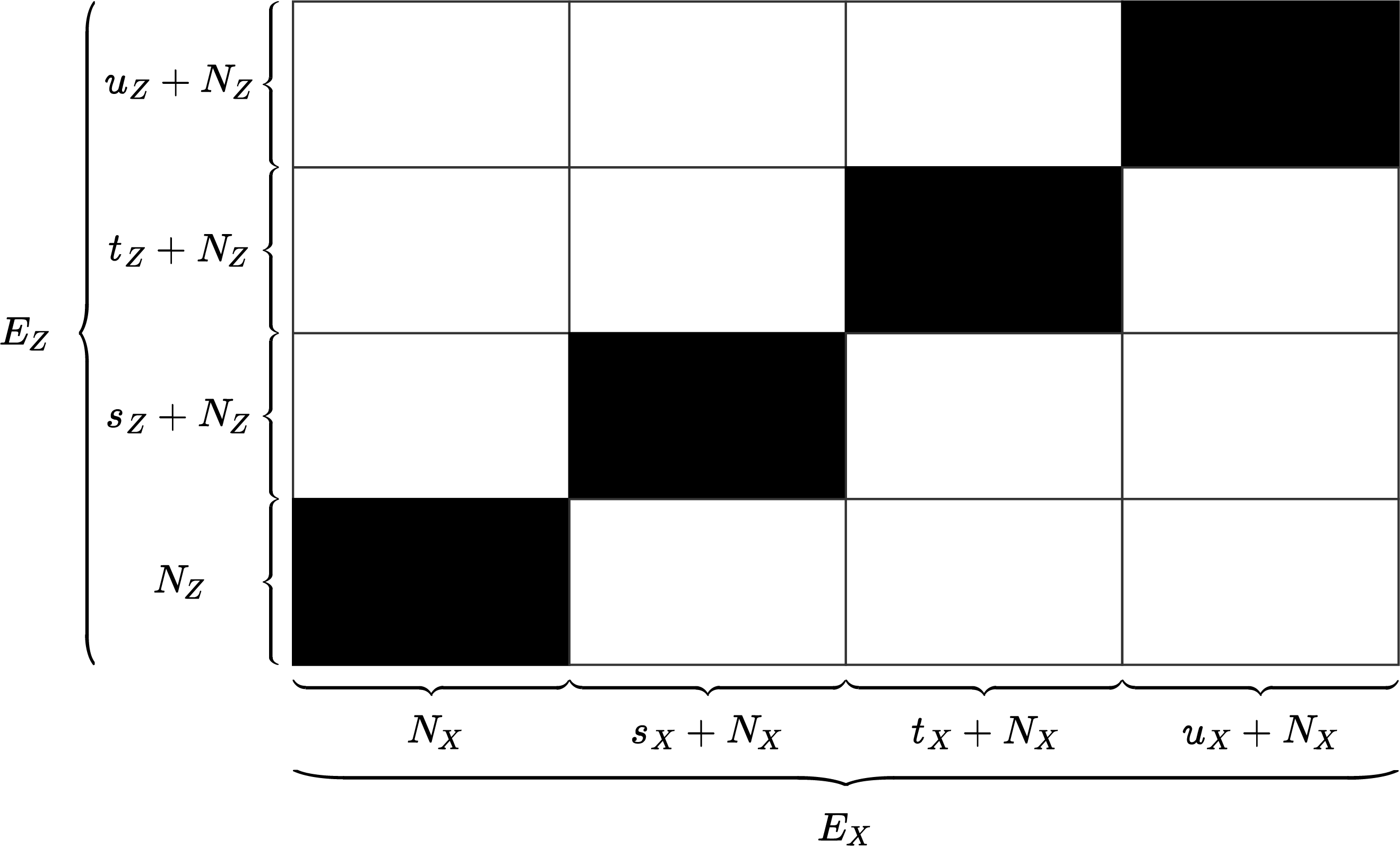
Figure 1: Illustration of Lemma 2 and Proposition 4 with $|{E_{X}}/{N_{X}}|=4=|{E_{Z}}/{N_{Z}}|$. Any subspace $H\leq G\times G$ consists of “blocks” — i.e., cosets — (dark shaded rectangles) of a direct product ${N_{X}}\times{N_{Z}}$ (bottom left dark shaded rectangle) contained inside a direct product ${E_{X}}\times{E_{Z}}$ (large rectangle). Shaded regions belong to $H$, while unshaded regions do not. Here, $\phi\left(v_{X}+{N_{X}}\right)=v_{Z}+{N_{Z}}$ for $v=s,t,u$.

As indicated in Eq. (94), the isomorphism $\phi$ specifies which $X$-type operators ${e_{X}^{j}}$ and $Z$-type operators ${e_{Z}^{j}}$ are “paired together” to form generators of $H$. We illustrate this in the following example.

Example 4 (5-qubit code).

The five-qubit code [52] is a stabilizer code, so its gauge group is the join of its stabilizer group and phases, $\mathcal{G}=\langle\mathcal{S},\Phi\rangle$.

Inspecting the stabilizer generators of this code in Eq. (58), we see that there are no elements of the gauge group that are purely $X$-type or $Z$-type. Thus, the internal code $N_{X}\times N_{Z}$ is trivial.

On the other hand, the external code $E_{X}\times E_{Z}$ is generated by splitting the gauge group into its $X$-part and $Z$-part. That is, with a slight abuse of notation, we have

$${E_{X}} =\langle IXXII,IIXXI,IIIXX,XIIIX\rangle\text{ and}$$ (95)

$${E_{Z}} =\langle ZIIZI,IZIIZ,ZIZII,IZIZI\rangle.$$ (96)

The isomorphism $\phi$ is constructed from combinations of ${e_{X}}\in{E_{X}}$ and ${e_{Z}}\in{E_{Z}}$ such that ${e_{X}}{e_{Z}}\in\mathcal{G}$. Thus, again with a slight abuse of notation, the action of $\phi$ is

$$IXXII \mapsto ZIIZI, IIXXI \mapsto IZIIZ,$$ (97)

$$IIIXX \mapsto ZIZII, XIIIX \mapsto IZIZI.$$ (98)

An alternative set of generators for the external code is

$${E_{X}} =\langle XXIII,IXXII,IIXXI,IIIXX\rangle\text{ and}$$ (99)

$${E_{Z}} =\langle ZZIII,IZZII,IIZZI,IIIZZ\rangle.$$ (100)

The external code can be gauged fixed to obtain the $[[5,1,0,3]]$ code. However, the external code has distance one, since $XIIII$ and $ZIIII$ are dressed logicals.

The Goursat data of a subsystem stabilizer code $H$ can be expressed explicitly in terms of its generators. This is useful for explicitly computing the Goursat data of subsystem stabilizer codes.

Proposition 5.

Suppose that

$$H=\left\langle\left({e_{X}^{1}},{e_{Z}^{1}}\right),\ldots,\left({e_{X}^{l}},{e_{Z}^{l}}\right)\right\rangle\leq G\times G.$$ (101)

Define the $\dim G\times l$ matrices

$$\pi_{X}\coloneqq\left(\begin{array}[]{ccc}|&&|\\ {e_{X}^{1}}&\ldots&{e_{X}^{l}}\\ |&&|\\ \end{array}\right)$$ (102)

and

$$\pi_{Z}\coloneqq\left(\begin{array}[]{ccc}|&&|\\ {e_{Z}^{1}}&\ldots&{e_{Z}^{l}}\\ |&&|\\ \end{array}\right).$$ (103)

Then

$$\begin{array}[]{ccccc}&&G\times G&&\\ G\times G&&|&&\\ |&\longleftrightarrow&\pi_{X}{\left(\mathbb{F}_{p}^{l}\right)}\times\pi_{Z}{\left(\mathbb{F}_{p}^{l}\right)}&,&\phi\\ H&&|&&\\ &&\pi_{X}{\left(\ker\pi_{Z}\right)}\times\pi_{Z}{\left(\ker\pi_{X}\right)}&&\end{array}$$ (104)

for some isomorphism $\phi$. Moreover, $H$ is a subsystem CSS code iff

$$\ker\pi_{X}+\ker\pi_{Z}=\mathbb{F}_{p}^{l}.$$ (105)

Proof.

See Appendix A.5. ∎

Note that Eq. (105) provides an alternative characterization of subsystem CSS codes that can be readily checked given the generators of $H$. Indeed, to check whether a given subsystem stabilizer code is a subsystem CSS code, one can compute spanning sets for $\ker\pi_{X}$ and $\ker\pi_{Z}$, take their union to form a spanning set for $\ker\pi_{X}+\ker\pi_{Z}$, and compare the dimension of that spanning set with $l$.

VI.2 Goursat data of the stabilizer group

The stabilizer group $H\cap H^{\omega}$ of a subsystem stabilizer code $H$ can be described in terms of the Goursat data of $H$. More broadly, our goal in this section is to determine the Goursat data of each subsystem stabilizer code in Eq. (33) in terms of the Goursat data of $H$, just as we determined the classical linear codes comprising each subsystem CSS code in Eq. (37) in terms of the classical linear codes comprising $H$.

We first derive the Goursat data of the gauge-preserving group $H^{\omega}$ in terms of that of $H$.

Proposition 6.

Suppose that

$$\begin{array}[]{ccccc}&&G\times G&&\\ G\times G&&|&&\\ |&\longleftrightarrow&{E_{X}}\times{E_{Z}}&,&\phi\\ H&&|&&\\ &&{N_{X}}\times{N_{Z}}&&\end{array}.$$ (106)

Then there exist isomorphisms $\phi_{X},\phi_{Z}$ in the diagram

$${N_{Z}^{\theta}}/{E_{Z}^{\theta}}\overset{\phi_{Z}}{\xrightarrow{\sim}}{E_{Z}}/{N_{Z}}\overset{\phi^{-1}}{\xrightarrow{\sim}}{E_{X}}/{N_{X}}\overset{\phi_{X}}{\xleftarrow{\sim}}{N_{X}^{\theta}}/{E_{X}^{\theta}},$$ (107)

such that with

$$\phi^{\omega}\coloneqq\phi_{X}^{-1}\phi^{-1}\phi_{Z},$$ (108)

we have

$$\begin{array}[]{ccccc}&&G\times G&&\\ G\times G&&|&&\\ |&\longleftrightarrow&N_{Z}^{\theta}\times N_{X}^{\theta}&,&\phi^{\omega}\\ H^{\omega}&&|&&\\ &&E_{Z}^{\theta}\times E_{X}^{\theta}&&\end{array}$$ (109)

Proof.

See Appendix A.6. ∎

Intuitively, this proposition states that if a subsystem stabilizer code $H$ corresponds to the subsystem CSS codes $N\leq H\leq E$, then the complement $H^{\omega}$ corresponds to the subsystem CSS codes $E^{\omega}\leq H^{\omega}\leq N^{\omega}$ (c.f. Eq. (21)).

Next, we derive the Goursat data of an intersection of codes $H\cap\tilde{H}$ in terms of the Goursat data of the original codes $H$ and $\tilde{H}$. This result is slightly more general than is needed to determine the Goursat data of the stabilizer $H\cap H^{\omega}$, since $\tilde{H}$ does not have to equal $H^{\omega}$.

Proposition 7.

Suppose that

$$\begin{array}[]{ccccc}&&G\times G&&\\ G\times G&&|&&\\ |&\longleftrightarrow&{E_{X}}\times{E_{Z}}&,&\phi\\ H&&|&&\\ &&{N_{X}}\times{N_{Z}}&&\end{array}$$ (110)

and

$$\begin{array}[]{ccccc}&&G\times G&&\\ G\times G&&|&&\\ |&\longleftrightarrow&\tilde{{E_{X}}}\times\tilde{{E_{Z}}}&,&\tilde{\phi}\\ \tilde{H}&&|&&\\ &&\tilde{{N_{X}}}\times\tilde{{N_{Z}}}&&\end{array}.$$ (111)

Then there exist subspaces

$$\begin{array}[]{ccccccc}{E_{X}}\cap\tilde{{E_{X}}}&&\left({E_{X}}/{N_{X}}\right)\times\left(\tilde{{E_{X}}}/\tilde{{N_{X}}}\right)&&\left({E_{Z}}/{N_{Z}}\right)\times\left(\tilde{{E_{Z}}}/\tilde{{N_{Z}}}\right)&&{E_{Z}}\cap\tilde{{E_{Z}}}\\ |&&|&&|&&|\\ T&,&\mathcal{U}&,&\mathcal{V}&,&W\\ |&&|&&|&&|\\ {N_{X}}\cap\tilde{{N_{X}}}&&0&&0&&{N_{Z}}\cap\tilde{{N_{Z}}}\\ \end{array}$$ (112)

and isomorphisms $\phi_{T},\phi_{W}$ in the diagram

$$T\left/\left({N_{X}}\cap\tilde{{N_{X}}}\right)\right.\overset{\phi_{T}}{\xrightarrow{\sim}}\mathcal{U}\overset{\phi\times\tilde{\phi}}{\xrightarrow{\sim}}\mathcal{V}\overset{\phi_{W}}{\xleftarrow{\sim}}W\left/\left({N_{Z}}\cap\tilde{{N_{Z}}}\right)\right.$$ (113)

such that with

$$\phi^{\cap}\coloneqq\phi_{W}^{-1}\left(\phi\times\tilde{\phi}\right)\phi_{T},$$ (114)

we have

$$\begin{array}[]{ccccc}&&G\times G&&\\ G\times G&&|&&\\ |&\longleftrightarrow&T\times W&,&\phi^{\cap}\\ H\cap\tilde{H}&&|&&\\ &&\left({N_{X}}\cap\tilde{{N_{X}}}\right)\times\left({N_{Z}}\cap\tilde{{N_{Z}}}\right)&&\end{array}.$$ (115)

Proof.

See Appendix A.7. ∎

Abstractly, Propositions 6 and 7 are sufficient to determine the Goursat data of each subsystem stabilizer code in Eq. (33) in terms of the Goursat data of $H$. However, these expressions for subsystem stabilizer codes are not as explicit as the expressions for subsystem CSS codes in Eq. (37). Nonetheless, Propositions 6 and 7 might be useful for some applications, such as a characterizaztion of subsystem stabilizer codes.

VI.3 Characterizing subsystem stabilizer codes using the Goursat data of the stabilizer group

Here, we characterize subsystem stabilizer codes according to the Goursat data of their stabilizer groups (see Fig. 2 for a summary).

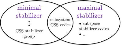
Figure 2: Venn diagram depicting features of subsystem stabilizer codes with maximal and minimal stabilizer groups, per Def. 4. A code has minimal stabilizer iff its stabilizer group is CSS. A code has minimal and maximal stabilizer iff its gauge group is CSS. Every subspace stabilizer code has maximal stabilizer, but there are codes with maximal stabilizer that are not subspace stabilizer codes.

Recall that a subsystem stabilizer code $H$ can equivalently be described by its Goursat data — the internal CSS code $N$, the external CSS code $E$, and the isomorphism $\phi$. Here, we are interested in the number of blocks in the stabilizer group $H\cap H^{\omega}$ of $H$ (see Figure 1). To motivate this inquiry, recall that the stabilizer group has one block iff it is CSS, and the stabilizer group has many blocks iff it is “far from CSS”. As we will show, the number of blocks in the stabilizer group is upper bounded by a function of $N$ and $E$. This upper bound is independent of the particular isomorphism $\phi$, which determines the true number of blocks in the stabilizer group of $H$. Thus, for fixed internal and external codes $N$ and $E$, we can define two extreme classes of codes which, in some sense, achieve the largest and the smallest number of blocks admitted by $N$ and $E$.

Definition 4.

Let

$$\begin{array}[]{ccccc}&&G\times G&&\\ G\times G&&|&&\\ |&\longleftrightarrow&{E_{X}}\times{E_{Z}}&,&\phi\\ H&&|&&\\ &&{N_{X}}\times{N_{Z}}&&\end{array}.$$ (116)

By Propositions 6 and 7, we have

$$\begin{array}[]{ccccc}&&\left({E_{X}}\cap{N_{Z}^{\theta}}\right)\times\left({E_{Z}}\cap{N_{X}^{\theta}}\right)&&\\ G\times G&&|&&\\ |&\longleftrightarrow&T\times W&,&\phi^{\cap}\\ H\cap H^{\omega}&&|&&\\ &&\left({N_{X}}\cap{E_{Z}^{\theta}}\right)\times\left({N_{Z}}\cap{E_{X}^{\theta}}\right)&&\end{array}$$ (117)

for some subspace $T\times W$ (interpreted as the external code of the stabilizer) and some isomorphism $\phi^{\cap}$. We say that $H$ has maximal stabilizer if

$$T\times W=\left({E_{X}}\cap{N_{Z}^{\theta}}\right)\times\left({E_{Z}}\cap{N_{X}^{\theta}}\right),$$ (118)

i.e., if $T\times W$ is as large as possible. We say that $H$ has minimal stabilizer if

$$T\times W=\left({N_{X}}\cap{E_{Z}^{\theta}}\right)\times\left({N_{Z}}\cap{E_{X}^{\theta}}\right),$$ (119)

i.e., if $T\times W$ is as small as possible.

It is in the following sense that subsystem stabilizer codes with maximal or minimal stabilizer generalize subsystem CSS codes.

Proposition 8.

A subsystem stabilizer code has both maximal and minimal stabilizer iff it is a subsystem CSS code.

Proof.

See Appendix A.8. ∎

Observe that a subsystem stabilizer code has minimal stabilizer iff its underlying stabilizer group is CSS. We remark that such codes have multiple characterizations.

Corollary 2.

The following are equivalent:

1. $H$ has minimal stabilizer

2. $H+H^{\omega}$ is a direct product

3. $H\cap H^{\omega}$ is a direct product

4. $H+H^{\omega}=({E_{X}}+{N_{Z}^{\theta}})\times({E_{Z}}+{N_{X}^{\theta}})$

5. $H\cap H^{\omega}=({N_{X}}\cap{E_{Z}^{\theta}})\times({N_{Z}}\cap{E_{X}^{\theta}})$

Proof.

By definition, (1) and (3) are equivalent. By Eq. (21), (2) and (3) are equivalent, and (4) and (5) are equivalent. By Propositions 6 and 7, (3) and (5) are equivalent. ∎

This corollary yields a simple algorithm to test whether a subsystem stabilizer code has minimal stabilizer. Indeed, given a spanning set for $H$, one can compute a spanning set for $H+H^{\omega}$ and apply Eq. (105) to test if $H+H^{\omega}$ is a direct product, i.e., if $H$ has minimal stabilizer. We leave a more detailed investigation of codes with maximal and minimal stabilizer for future research.

VII Conclusion

In this work, we study subsystem stabilizer codes in a linear algebraic framework by viewing Pauli groups as vector spaces and subsystem stabilizer codes as subspaces via the symplectic representation. This perspective allows us to construct a doubling map that converts any modular-qudit subsystem stabilizer code into a subsystem CSS code with comparable parameters (see Theorem 1).

The linear algebraic perspective also elucidates the correspondence between a subsystem CSS code and a pair of classical linear codes, yielding an explicit basis of codewords (see Section III), a generalized Steane-type recovery procedure (see Section V), and other results (see Appendices C and D).

Finally, the linear-algebraic perspective enables a characterization of subsystem stabilizer codes via Goursat’s Lemma, which yields two generalizations of subsystem CSS codes (see Section VI).

We conclude with questions and outlook for future investigations.

1. Is our “doubling” map from $[[n,k,r,d]]$ subsystem stabilizer codes to $[[2n,2k,2r,d\leq d^{\prime}\leq 2d]]$ subsystem CSS codes in Theorem 1 tight in terms of the required number of physical qudits?

2. Which subsystem stabilizer codes yield “doubled” subsystem CSS codes with exactly twice the code distance?

3. Does our recovery procedure in Section V interact nicely with the “doubled” subsystem CSS code?

4. Keeping in mind that Steane error correction is fault-tolerant for subspace codes, can our subsystem syndrome extraction procedure in Section V.1 be made fault-tolerant?

5. Does the Goursat-based characterization in Section VI.1 simplify significantly for subspace stabilizer codes?

6. How does the Goursat data of a code behave under Clifford deformations?

7. Is there a concise characterization of subsystem stabilizer codes with maximal (minimal) stabilizer, as introduced in Definition 4?

8. Do subsystem stabilizer codes with maximal (minimal) stabilizer have nice structural properties, analogous to those described in Proposition 2 for subsystem CSS codes?

9. Our doubling map holds for all modular-qudit subsystem stabilizer codes — can we generalize our other results to codes over modular qudits or operator algebra stabilizer codes [50, 47] ?

10. Using existing (non-CSS) Floquet codes [63, 64, 65, 66, 67, 68, 69] , new CSS Floquet codes [70, 71, 72, 73, 74] can be constructed using our mapping. Such CSS codes could be more amenable to the analysis of fault-tolerance using ZX calculus [73, 65, 74].

Appendix A Proofs of Propositions

A.1 Proof of Proposition 1

Write

$$\overline{H} \coloneqq\left(H+H^{\omega}\right)/H\text{ and}$$ (120)

$$\underline{H} \coloneqq H/\left(H\cap H^{\omega}\right).$$ (121)

One verifies that the map

$$\left(a+\left(H\cap H^{\omega}\right),b+\left(H\cap H^{\omega}\right)\right)\mapsto\omega(a,b)$$ (122)

is an antisymmetric form on $\underline{H}$. Since every vector space with an antisymmetric form has even dimension [34], we have $\dim\underline{H}=2r$ for some $r\in\mathbb{Z}$. Moreover, observe that

$$\dim\overline{H}+\dim\underline{H} =\dim H+H^{\omega}-\dim H\cap H^{\omega}$$ (123)

$$=\dim G\times G-2\dim H\cap H^{\omega},$$

so $\dim\overline{H}=2k$ for some $k\in\mathbb{Z}$. Next, note that

$$\dim G\times G-\dim\left(H+H^{\omega}\right)=\dim\left(H\cap H^{\omega}\right).$$ (124)

Since the dimensions in Eq. (33) must sum to $\dim G\times G=2n$, we find that $\dim H\cap H^{\omega}=n-k-r$, as needed. The final statement follows by defining $d$ appropriately.

A.2 Proof of Proposition 2

First, note that Eq. (37) follows directly from Eq. (21). Next, observe that

$$\dim{\left(H_{X}+H_{Z}^{\theta}\right)}/H_{X} =\dim H_{X}^{\theta}/\left(H_{Z}\cap H_{X}^{\theta}\right)$$ (125)

$$=\dim{\left(H_{Z}+H_{X}^{\theta}\right)}/H_{Z}$$

and

$$\dim H_{X}/{\left(H_{X}\cap H_{Z}^{\theta}\right)} =\dim{\left(H_{Z}+H_{X}^{\theta}\right)}/H_{X}^{\theta}$$ (126)

$$=\dim H_{Z}/{\left(H_{Z}\cap H_{X}^{\theta}\right)},$$

so the claim about dimensions follows. Finally, recall that

$$d\coloneqq\min\operatorname{swt}\left({\left(H+H^{\omega}\right)}\setminus H\right).$$ (127)

Fix $(a,b)\in{\left(H+H^{\omega}\right)}\setminus H$ with $\operatorname{swt}(a,b)=d$. Then $a\in{\left(H_{X}+H_{Z}^{\theta}\right)}$ and $b\in{\left(H_{Z}+H_{X}^{\theta}\right)}$, but either $a\notin H_{X}$ or $b\notin H_{Z}$. If $a\notin H_{X}$, then

$$d=\operatorname{swt}(a,b)\geq\operatorname{swt}(a,0)=\operatorname{wt}(a)\geq d^{H_{X}}.$$ (128)

If instead $b\notin H_{Z}$, a similar argument shows that $d\geq d^{H_{Z}}$. Conversely, suppose that $a\in\left(H_{X}+H_{Z}^{\theta}\right)\setminus H_{X}$ satisfies $\operatorname{wt}(a)=\min\left\{d^{H_{X}},d^{H_{Z}}\right\}$. Then

$$d\leq\operatorname{swt}(a,0)=\operatorname{wt}(a)=\min\left\{d^{H_{X}},d^{H_{Z}}\right\}.$$ (129)

If instead $b\in{\left(H_{Z}+H_{X}^{\theta}\right)}\setminus H_{Z}$ satisfies $\operatorname{wt}(b)=\min\left\{d^{H_{X}},d^{H_{Z}}\right\}$, a similar argument shows that $d\leq\min\left\{d^{H_{X}},d^{H_{Z}}\right\}$.

A.3 Proof of Proposition 3

Since we know $Fa$, we can determine $a+K$ by the first isomorphism theorem. By assumption, there exists $r\in R$ such that $\operatorname{wt}(a+r)<\frac{d^{R}}{2}$. Thus, we can identify some $a+k\in a+K$ with $\operatorname{wt}(a+k)<\frac{d^{R}}{2}$, where $k\in K$ is unknown. By the triangle inequality, we have

$$\operatorname{wt}(r-k) =\operatorname{wt}((a+r)-(a+k))$$ (130)

$$\leq\operatorname{wt}(a+r)+\operatorname{wt}(a+k)$$

$$<d^{R}$$

$$=\min\operatorname{wt}(K\setminus R).$$

Thus, since $r-k\in K$, we must have $r-k\in R$, so $k\in R$.

A.4 Proof of Proposition 4

On the one hand, observe that

$$\phi\left(\sum_{j}c_{j}{e_{X}^{j}}+{n_{X}}+{N_{X}}\right) =\sum_{j}c_{j}\phi\left({e_{X}^{j}}+{N_{X}}\right)$$ (131)

$$=\sum_{j}c_{j}\left({e_{Z}^{j}}+{N_{Z}}\right)$$

$$=\sum_{j}c_{j}{e_{Z}^{j}}+{n_{Z}}+{N_{Z}}.$$

Conversely, suppose that $\left({e_{X}},{e_{Z}}\right)\in{E_{X}}\times{E_{Z}}$ satisfies $\phi\left({e_{X}}+{N_{X}}\right)={e_{Z}}+{N_{Z}}$. Write

$${e_{X}}+{N_{X}}=\sum_{j}c_{j}\left({e_{X}^{j}}+{N_{X}}\right)$$ (132)

and

$${e_{Z}}+{N_{Z}}=\sum_{j}d_{j}\left({e_{Z}^{j}}+{N_{Z}}\right)$$ (133)

for some $c_{j},d_{j}\in\mathbb{F}_{p}$. Then

$$\sum_{j}c_{j}\left({e_{Z}^{j}}+{N_{Z}}\right)=\sum_{j}d_{j}\left({e_{Z}^{j}}+{N_{Z}}\right),$$ (134)

so $c_{j}=d_{j}$ for all $j$. Then

$${e_{X}}=\sum_{j}c_{j}{e_{X}^{j}}+{n_{X}}$$ (135)

and

$${e_{Z}}=\sum_{j}c_{j}{e_{Z}^{j}}+{n_{Z}}$$ (136)

for some ${n_{X}}\in{N_{X}}$ and ${n_{Z}}\in{N_{Z}}$, so Eq. (94) holds.

A.5 Proof of Proposition 5

One verifies Eq. (104) from the definitions in Eq. (84). To prove Eq. (105), we need the following technical lemma.

Lemma 3.

Let $W\leq V\leq U$, and let $\pi:U\to X$ be any linear map. Then $\pi(W)=\pi(V)$ iff $(V\cap\ker\pi)+W=V$.

Proof.

Suppose that $\pi(W)=\pi(V)$. Fix $v\in V$. Then there exists $w\in W$ such that $\pi(v)=\pi(w)$. Then $v=(v-w)+w$, where $v-w\in V\cap\ker\pi$. Conversely, suppose that $(V\cap\ker\pi)+W=V$. Fix $v\in V$. Then there exist $k\in V\cap\ker\pi$ and $w\in W$ such that $v=k+w$. Then $\pi(v)=\pi(w)$. Thus, $\pi(V)\subseteq\pi(W)$, as needed. ∎

Now, recall that $H$ is a direct product iff $\pi_{X}{\left(\ker\pi_{Z}\right)}=\pi_{X}{\left(\mathbb{F}_{p}^{l}\right)}$. Applying the above lemma with $U=V=\mathbb{F}_{p}^{l}$, $W=\ker\pi_{Z}$, and $\pi=\pi_{X}$, we obtain Eq. (105).

A.6 Proof of Proposition 6

Fix a basis $\left\{{e_{X}^{j}}+{N_{X}}\right\}_{j}$ for ${E_{X}}/{N_{X}}$. Define the function

$$\tilde{\phi}_{X}:{N_{X}^{\theta}} \to{E_{X}}/{N_{X}}$$ (137)

$${n_{X}^{\theta}} \mapsto\sum_{j}\theta\left({e_{X}^{j}},{n_{X}^{\theta}}\right)\left({e_{X}^{j}}+{N_{X}}\right).$$

Since ${n_{X}^{\theta}}\in{N_{X}^{\theta}}$, the function $\tilde{\phi}_{X}$ is independent of the choice of representatives ${e_{X}^{j}}$ for the cosets ${e_{X}^{j}}+{N_{X}}$. Since $\theta$ is bilinear, $\tilde{\phi}_{X}$ is linear. Now, if ${n_{X}^{\theta}}\in{E_{X}^{\theta}}$, then $\tilde{\phi}_{X}\left({n_{X}^{\theta}}\right)={N_{X}}$. Conversely, suppose that $\tilde{\phi}_{X}\left({n_{X}^{\theta}}\right)={N_{X}}$. Since the ${e_{X}^{j}}+{N_{X}}$ are linearly independent, we have $\theta\left({e_{X}^{j}},{n_{X}^{\theta}}\right)=0$ for all $j$. Since every ${e_{X}}\in{E_{X}}$ can be written as

$${e_{X}}=\sum_{j}c_{j}{e_{X}^{j}}+{n_{X}}$$ (138)

for some $c_{j}\in\mathbb{F}_{p}$ and ${n_{X}}\in{N_{X}}$, we find that ${n_{X}^{\theta}}\in{E_{X}^{\theta}}$. Thus, $\ker\tilde{\phi}_{X}={E_{X}^{\theta}}$. Then $\tilde{\phi}_{X}$ induces the injection

$$\phi_{X}:{N_{X}^{\theta}}/{E_{X}^{\theta}} \to{E_{X}}/{N_{X}}$$ (139)

$${n_{X}^{\theta}}+{E_{X}^{\theta}} \mapsto\tilde{\phi}_{X}\left({n_{X}^{\theta}}\right).$$

In fact, since $\dim{N_{X}^{\theta}}/{E_{X}^{\theta}}=\dim{E_{X}}/{N_{X}}$, the map $\phi_{X}$ is an isomorphism.

Similarly, given the basis

$$\left\{\phi\left({e_{X}^{j}}+{N_{X}}\right)\eqqcolon{e_{Z}^{j}}+{N_{Z}}\right\}_{j}$$ (140)

for ${E_{Z}}/{N_{Z}}$, there exists an isomorphism $\phi_{Z}:{N_{Z}^{\theta}}/{E_{Z}^{\theta}}\to{E_{Z}}/{N_{Z}}$, where

$$\phi_{Z}\left({n_{Z}^{\theta}}+{E_{Z}^{\theta}}\right)\coloneqq\sum_{j}\theta\left({e_{Z}^{j}},{n_{Z}^{\theta}}\right)\left({e_{Z}^{j}}+{N_{Z}}\right).$$ (141)

Now, define $\phi^{\omega}\coloneqq\phi_{X}^{-1}\phi^{-1}\phi_{Z}$. Fix $\left({n_{Z}^{\theta}},{n_{X}^{\theta}}\right)\in{N_{Z}^{\theta}}\times{N_{X}^{\theta}}$. By definition, we have

$$\phi^{\omega}\left({n_{Z}^{\theta}}+{E_{Z}^{\theta}}\right)={n_{X}^{\theta}}+{E_{X}^{\theta}}$$ (142)

iff

$$\phi_{Z}\left({n_{Z}^{\theta}}+{E_{Z}^{\theta}}\right)=\phi\left(\phi_{X}\left({n_{X}^{\theta}}+{E_{X}^{\theta}}\right)\right).$$ (143)

By Eqs. (139) and (141), this is equivalent to

$$\sum_{j}\theta\left({e_{Z}^{j}},{n_{Z}^{\theta}}\right) \left({e_{Z}^{j}}+{N_{Z}}\right)$$ (144)

$$={} \phi\left(\sum_{j}\theta\left({e_{X}^{j}},{n_{X}^{\theta}}\right)\left({e_{X}^{j}}+{N_{X}}\right)\right),$$

which is equivalent to

$$\sum_{j}\theta\left({e_{Z}^{j}},{n_{Z}^{\theta}}\right){} \phi\left({e_{X}^{j}}+{N_{X}}\right)$$ (145)

$$=\sum_{j}{} \theta\left({e_{X}^{j}},{n_{X}^{\theta}}\right)\phi\left({e_{X}^{j}}+{N_{X}}\right).$$

Since the $\phi\left({e_{X}^{j}}+{N_{X}}\right)$ are linearly independent, this is equivalent to

$$\forall j,\,\theta\left({e_{Z}^{j}},{n_{Z}^{\theta}}\right)=\theta\left({e_{X}^{j}},{n_{X}^{\theta}}\right),$$ (146)

which by Eq. (94) is equivalent to

$$\forall\left({e_{X}},{e_{Z}}\right)\in H,\,\theta\left({e_{Z}},{n_{Z}^{\theta}}\right)=\theta\left({e_{X}},{n_{X}^{\theta}}\right).$$ (147)

Rewriting, this occurs iff

$$\forall\left({e_{X}},{e_{Z}}\right)\in H,\,\omega\left(\left({e_{X}},{e_{Z}}\right),\left({n_{Z}^{\theta}},{n_{X}^{\theta}}\right)\right)=0,$$ (148)

which is equivalent to $\left({n_{Z}^{\theta}},{n_{X}^{\theta}}\right)\in H^{\omega}$. Now, since ${N_{X}}\times{N_{Z}}\leq H$, we have $H^{\omega}\leq{N_{Z}^{\theta}}\times{N_{X}^{\theta}}$. Thus, we find

$$H^{\omega}=\left\{\left({n_{Z}^{\theta}},{n_{X}^{\theta}}\right)\in{N_{Z}^{\theta}}\times{N_{X}^{\theta}}\,\middle|\,\phi^{\omega}\left({n_{Z}^{\theta}}+{E_{Z}}^{\theta}\right)={n_{X}^{\theta}}+{E_{X}^{\theta}}\right\},$$ (149)

as needed.

A.7 Proof of Proposition 7

Consider the injections $\phi_{T},\phi_{W}$ defined in the diagram

$$\begin{array}[]{ccccccc}\left({E_{X}}\cap\tilde{{E_{X}}}\right)/\left({N_{X}}\cap\tilde{{N_{X}}}\right)&\overset{\phi_{T}}{\hookrightarrow}&\left({E_{X}}/{N_{X}}\right)\times\left(\tilde{{E_{X}}}/\tilde{{N_{X}}}\right)&\overset{\phi\times\tilde{\phi}}{\xrightarrow{\sim}}&\left({E_{Z}}/{N_{Z}}\right)\times\left(\tilde{{E_{Z}}}/\tilde{{N_{Z}}}\right)&\overset{\phi_{W}}{\hookleftarrow}&\left({E_{Z}}\cap\tilde{{E_{Z}}}\right)/\left({N_{Z}}\cap\tilde{{N_{Z}}}\right)\\ a+\left({N_{X}}\cap\tilde{{N_{X}}}\right)&{\mapsto}&\left(a+{N_{X}},a+\tilde{{N_{X}}}\right)&&\left(b+{N_{Z}},b+\tilde{{N_{Z}}}\right)&{\mapsfrom}&b+\left({N_{Z}}\cap\tilde{{N_{Z}}}\right)\end{array}.$$ (150)

Moving “left to right” in the above diagram, define

$$\mathcal{W}\coloneqq\phi_{W}^{-1}\left(\phi\times\tilde{\phi}\right)\phi_{T}\left(\left({E_{X}}\cap\tilde{{E_{X}}}\right)/\left({N_{X}}\cap\tilde{{N_{X}}}\right)\right).$$ (151)

Moving “right to left” in the above diagram, define

$$\mathcal{V} \coloneqq\phi_{W}(\mathcal{W}),$$ (152)

$$\mathcal{U} \coloneqq\left(\phi\times\tilde{\phi}\right)^{-1}(\mathcal{V}),$$ (153)

$$\mathcal{T} \coloneqq\phi_{T}^{-1}(\mathcal{U}).$$ (154)

From the definitions, it is straightforward to verify that the appropriate restrictions of $\phi_{T},\phi\times\tilde{\phi},\phi_{W}$ satisfy

$$\begin{array}[]{ccccccc}\mathcal{T}&\overset{\phi_{T}}{\xrightarrow{\sim}}&\mathcal{U}&\overset{\phi\times\tilde{\phi}}{\xrightarrow{\sim}}&\mathcal{V}&\overset{\phi_{W}}{\xleftarrow{\sim}}&\mathcal{W}\\ \end{array}.$$ (155)

By the lattice isomorphism theorem, there exist subspaces

$$\begin{array}[]{ccc}{E_{X}}\cap\tilde{{E_{X}}}&&{E_{Z}}\cap\tilde{{E_{Z}}}\\ |&&|\\ T&\text{and}&W\\ |&&|\\ {N_{X}}\cap\tilde{{N_{X}}}&&{N_{Z}}\cap\tilde{{N_{Z}}}\\ \end{array}$$ (156)

such that

$$\mathcal{T} =T\left/\left({N_{X}}\cap\tilde{{N_{X}}}\right)\right.\text{and}$$ (157)

$$\mathcal{W} =W\left/\left({N_{Z}}\cap\tilde{{N_{Z}}}\right).\right.$$

Now, fix $(a,b)\in T\times W$. Then with

$$\phi^{\cap}\coloneqq\phi_{W}^{-1}\left(\phi\times\tilde{\phi}\right)\phi_{T},$$ (158)

we have

$$\phi^{\cap}\left(a+\left({N_{X}}\cap\tilde{{N_{X}}}\right)\right)=b+\left({N_{Z}}\cap\tilde{{N_{Z}}}\right)$$ (159)

iff

$$\left(\phi\times\tilde{\phi}\right)\phi_{T}\left(a+\left({N_{X}}\cap\tilde{{N_{X}}}\right)\right)=\phi_{W}\left(b+\left({N_{Z}}\cap\tilde{{N_{Z}}}\right)\right),$$ (160)

which occurs iff

$$\left(\phi\times\tilde{\phi}\right)\left(a+{N_{X}},a+\tilde{{N_{X}}}\right)=\left(b+{N_{Z}},b+\tilde{{N_{Z}}}\right).$$ (161)

Reading coordinate-wise, this occurs iff

$$\phi\left(a+{N_{X}}\right) =b+{N_{Z}}\text{ and}$$ (162)

$$\tilde{\phi}\left(a+\tilde{{N_{X}}}\right) =b+\tilde{{N_{Z}}},$$

which occurs iff

$$(a,b)\in H\text{ and }(a,b)\in\tilde{H}.$$ (163)

Moreover, if $(a,b)\in H\cap\tilde{H}\subseteq{E_{X}}\cap\tilde{{E_{X}}}$, then by the same computation above, we find

$$\left(\phi\times\tilde{\phi}\right)\left(\phi_{T}\left(a+\left({N_{X}}\cap\tilde{{N_{X}}}\right)\right)\right)$$ (164)

$$=\phi_{W}\left(b+\left({N_{Z}}\cap\tilde{{N_{Z}}}\right)\right)$$ .

That is, $b+\left({N_{Z}}\cap\tilde{{N_{Z}}}\right)\in\mathcal{W}$, so $a+\left({N_{X}}\cap\tilde{{N_{X}}}\right)\in\mathcal{T}$. Then $(a,b)\in T\times W$, so $H\cap\tilde{H}\subseteq T\times W$. Thus, we have

$$H\cap\tilde{H}=\Big{\{}(a,b)\in T\times W\,\Big{|}\,\phi^{\cap}\Big{(} a+\Big{(}{N_{X}}\cap\tilde{{N_{X}}}\Big{)}\Big{)}$$ (165)

$$={} b+\Big{(}{N_{Z}}\cap\tilde{{N_{Z}}}\Big{)}\Big{\}},$$

as needed.

A.8 Proof of Proposition 8

Suppose that $H$ has both maximal and minimal stabilizer. Taking orthogonal complements in the right-hand side factor, we have

$${N_{X}}\cap{E_{Z}^{\theta}} ={E_{X}}\cap{N_{Z}^{\theta}}\text{ and}$$ (166)

$${E_{X}}+{N_{Z}^{\theta}} ={N_{X}}+{E_{Z}^{\theta}}.$$ (167)

On the one hand,

$$\dim{E_{X}}+\dim{N_{Z}^{\theta}} =\dim\left({E_{X}}+{N_{Z}^{\theta}}\right)+\dim\left({E_{X}}\cap{N_{Z}^{\theta}}\right)$$ (168)

$$=\dim\left({N_{X}}+{E_{Z}^{\theta}}\right)+\dim\left({N_{X}}\cap{E_{Z}^{\theta}}\right)$$

$$=\dim{N_{X}}+\dim{E_{Z}^{\theta}}.$$

On the other hand,

$$\dim{E_{X}} \geq\dim{N_{X}}\text{ and}$$ (169)

$$\dim{N_{Z}^{\theta}} \geq\dim{E_{Z}^{\theta}}.$$ (170)

Thus, we have

$${E_{X}}={N_{X}}\text{ and }{E_{Z}}={N_{Z}},$$ (171)

as needed. The converse is clear — assume Eq. (171) and simplify the right-hand side of Eq. (117).

Appendix B Generalizing Theorem 1 to subsystem stabilizer codes over modular qudits

In this appendix, we briefly describe how to generalize Theorem 1 to subsystem stabilizer codes over modular qudits. The material in the preliminaries, Section II, generalizes as follows [47, 34, 10].

• The prime $p$ is now an arbitrary integer $m$, so $G$ is now the finite abelian group $\left(\mathbb{Z}/m\mathbb{Z}\right)^{n}$ with standard generating set $\{(1,0,\ldots,0),\ldots,(0,\ldots,0,1)\}$

• The Pauli group modulo phases is still isomorphic to $G\times G$

• Eq. (14) now reads as $\left|H\right|\left|H^{\xi}\right|=\left|G\right|$, where the absolute value denotes group order

• A subsystem stabilizer code is now a subgroup $H\leq G\times G$. We call $H$ a subsystem CSS code if $H$ is a direct product of subgroups of $G$

• We no longer keep track of the number of logical and gauge qudits in a subsystem stabilizer code. Rather, we keep track of the logical Pauli group $\overline{H}\coloneqq\left(H+H^{\omega}\right)/H$ and the gauge Pauli group $\underline{H}\coloneqq H/\left(H\cap H^{\omega}\right)$ — see Eqs. (31) and (32). The logical (resp. gauge) Pauli group is isomorphic to the group of Pauli operators on the logical (resp. gauge) subsystem $\mathbb{L}$ (resp. $\mathbb{G}$) [10]

Having established the necessary background, we now sketch the generalization of Theorem 1.

• Eq. (44d) in Lemma 1 now reads as $\left|\Delta(H)\right|=\left|H\right|^{2}$, and the analogue of Lemma 1 holds with essentially the same proof

• Theorem 1 now reads as follows, where the proof is similar

Theorem 2.

Let $H\leq G\times G$ be a subsystem stabilizer code with logical Pauli group $\overline{H}$, gauge Pauli group $\underline{H}$, and distance $d$. Then $\Delta(H)$ is a subsystem CSS code with logical Pauli group isomorphic to $\overline{H}\times\overline{H}$, gauge Pauli group isomorphic to $\underline{H}\times\underline{H}$, and distance $d^{\prime}$, where $d\leq d^{\prime}\leq 2d$. Moreover, if $H$ admits a collection of generators with symplectic weight at most $w$, then $\Delta(H)$ admits a collection of generators with symplectic weight at most $2w$.

Appendix C An alternative classical step for error recovery

In this appendix, we explore an alternative to the classical step for error recovery described in Section V.2. To begin, consider the commutative diagram of canonical quotients

$$\leavevmode\hbox to133.15pt{\vbox to86.07pt{\text{[drawing]}}}. {G} {G/{\left(H_{X}+H_{Z}^{\theta}\right)}} {G/H_{X}} \scriptstyle{\overline{*}} \scriptstyle{\operatorname{Syn}_{X}} \scriptstyle{\operatorname{Par}_{X}} {G} {G/{\left(H_{X}+H_{Z}^{\theta}\right)}} {G/H_{X}} \scriptstyle{\overline{*}} \scriptstyle{\operatorname{Syn}_{X}} \scriptstyle{\operatorname{Par}_{X}}$$ (172)

In Section V.2, we used the parity check $\operatorname{Syn}_{X}$ of the classical linear code $H_{X}+H_{Z}^{\theta}$ to recover an error class $a+H_{X}$ from its syndrome $a+\left(H_{X}+H_{Z}^{\theta}\right)$. Here, we investigate the utility of $\operatorname{Par}_{X}$ for the same task — this line of inquiry is motivated by the Bacon–Shor decoder [30], which utilizes $\operatorname{Par}_{X}$ for error recovery (see Example 5). We will need the following notation.

Let $\sigma\subseteq G$ denote the standard basis for $G$. Let $\sigma_{0}$ be any subset of $\sigma$ such that $\overline{\sigma_{0}}$ is a basis for $G/H_{X}$, where the over-line denotes quotient by $H_{X}$. For any $a+H_{X}\in G/H_{X}$, we write $\operatorname{wt}_{\overline{\sigma_{0}}}(a+H_{X})$ to denote the weight of $a+H_{X}$ in the basis $\overline{\sigma_{0}}$, i.e., the number of nonzero coordinates of $a+H_{X}$ in the basis $\overline{\sigma_{0}}$.

Now, recall that by Proposition 3, $\operatorname{Syn}_{X}$ can recover the error class $a+H_{X}$ from its syndrome $a+\left(H_{X}+H_{Z}^{\theta}\right)$ provided that

$$\min\operatorname{wt}(a+H_{X})<\frac{d^{H_{X}}}{2}.$$ (173)

Similarly, $\operatorname{Par}_{X}$ can recover the error $a+H_{X}$ from its syndrome $a+\left(H_{X}+H_{Z}^{\theta}\right)$ provided that

$$\operatorname{wt}_{\overline{\sigma_{0}}}\left(a+H_{X}\right)<\frac{d^{\operatorname{Par}_{X}}}{2},$$ (174)

where

$$d^{\operatorname{Par}_{X}}\coloneqq\min\operatorname{wt}_{\overline{\sigma_{0}}}\left({\left(H_{X}+H_{Z}^{\theta}\right)}/H_{X}\right)$$ (175)

is the distance of $\operatorname{Par}_{X}$ in the basis $\overline{\sigma_{0}}$. Our first observation is that the notions of weight and distance in Eqs. (173) and (174) are related.

Proposition 9.

We have

$$\min\operatorname{wt}(a+H_{X})\leq\operatorname{wt}_{\overline{\sigma_{0}}}\left(a+H_{X}\right)$$ (176)

for all $a\in G$. Moreover, we have

$$d^{H_{X}}\leq d^{\operatorname{Par}_{X}}.$$ (177)

Proof.

First, note that for any $a\in G$, we have

$$a+H_{X}=\sum_{\alpha\in{\sigma_{0}}}a_{\alpha}\left(\alpha+H_{X}\right)$$ (178)

for some $a_{\alpha}\in\mathbb{F}_{p}$, so

$$a+h_{X}=\sum_{\alpha\in{\sigma_{0}}}a_{\alpha}\alpha$$ (179)

for some $h_{X}\in H_{X}$. Thus,

$$\min\operatorname{wt}(a+H_{X})\leq\operatorname{wt}(a+h_{X})=\operatorname{wt}_{\overline{\sigma_{0}}}\left(a+H_{X}\right).$$ (180)

Now, suppose in addition that $a+H_{X}\in{\left(H_{X}+H_{Z}^{\theta}\right)}/H_{X}$ is nonzero and satisfies $\operatorname{wt}_{\overline{\sigma_{0}}}\left(a+H_{X}\right)=d^{\operatorname{Par}_{X}}$. Then $a+h_{X}\in{\left(H_{X}+H_{Z}^{\theta}\right)}\setminus H_{X}$, so

$$d^{H_{X}}\leq\operatorname{wt}(a+h_{X})=\operatorname{wt}_{\overline{\sigma_{0}}}\left(a+H_{X}\right)=d^{\operatorname{Par}_{X}}.$$ (181)

∎

Unfortunately, this proposition does not immediately reveal whether $\operatorname{Par}_{X}$ performs better or worse than $\operatorname{Syn}_{X}$. Indeed, the distance of $\operatorname{Par}_{X}$ is nominally lower bounded by the distance of $\operatorname{Syn}_{X}$, but the notion of error weight relevant for $\operatorname{Par}_{X}$ is also lower bounded by that for $\operatorname{Syn}_{X}$. Thus, it is not immediately clear whether one code performs better than the other. To shed light on this issue, we investigate the special case in which the notions of error weight for $\operatorname{Par}_{X}$ and $\operatorname{Syn}_{X}$ coincide.

Definition 5.

We say that $H_{X}\leq G$ respects weight if there exists $\sigma_{0}\subseteq\sigma$ such that $\overline{\sigma_{0}}$ is a basis for $G/H_{X}$ satisfying

$$\min\operatorname{wt}(a+H_{X})=\operatorname{wt}_{\overline{\sigma_{0}}}\left(a+H_{X}\right)$$ (182)

for all $a\in G$.

Note that by definition, $H_{X}$ respects weight iff the notions of weight for $\operatorname{Syn}_{X}$ and $\operatorname{Par}_{X}$ in Eqs. (173) and (174) coincide. In fact, if $H_{X}$ respects weight, then the distances of $\operatorname{Syn}_{X}$ and $\operatorname{Par}_{X}$ also coincide. To see this, note that

$$d^{\operatorname{Par}_{X}} =\underset{a\in(H_{X}+H_{Z}^{\theta})\setminus H_{X}}{\min}\operatorname{wt}_{\overline{\sigma_{0}}}\left(a+H_{X}\right)$$ (183)

$$\leq\underset{a\in(H_{X}+H_{Z}^{\theta})\setminus H_{X}}{\min}\operatorname{wt}(a)$$

$$=d^{H_{X}},$$

so by Proposition 9, we have $d^{H_{X}}=d^{\operatorname{Par}_{X}}$.

Interestingly, it turns out that there are not very many subspaces $H_{X}\leq G$ that respect weight.

Proposition 10.

A subspace $H_{X}\leq G$ respects weight iff $H_{X}$ admits a basis whose elements have weight at most $2$.

Proof.

$(\implies)$ Fix $\beta\in\sigma_{0}^{c}\coloneqq\sigma\setminus\sigma_{0}$ and write

$$\beta+H_{X}=\sum_{\alpha\in{\sigma_{0}}}a_{\alpha\beta}\left(\alpha+H_{X}\right),$$ (184)

where the $a_{\alpha\beta}\in\mathbb{F}_{p}$. If more than one $a_{\alpha\beta}$ is nonzero, then $\operatorname{wt}_{\overline{\sigma_{0}}}\left(\beta+H_{X}\right)>1$ but $\operatorname{wt}(\beta)=1$, a contradiction. Thus, at most one $a_{\alpha\beta}$ is nonzero, so $\beta=b_{\beta}\alpha_{\beta}+\gamma_{\beta}$ for some $b_{\beta}\in\mathbb{F}_{p}$, $\alpha_{\beta}\in\sigma_{0}$ and $\gamma_{\beta}\in H_{X}$. We claim that $\Gamma\coloneqq\left\{\gamma_{\beta}\,\middle|\,\beta\in\sigma_{0}^{c}\right\}\subseteq H_{X}$ is linearly independent. Indeed, suppose that

$$\sum_{\beta\in\sigma_{0}^{c}}c_{\beta}\gamma_{\beta}=0$$ (185)

for some $c_{\beta}\in\mathbb{F}_{p}$. Then

$$\sum_{\beta\in\sigma_{0}^{c}}c_{\beta}\beta=\sum_{\beta\in\sigma_{0}^{c}}c_{\beta}b_{\beta}\alpha_{\beta},$$ (186)

which by linear independence of $\sigma$ implies that $c_{\beta}=0$ for all $\beta\in\sigma_{0}^{c}$. Thus, $\Gamma$ has exactly $\left|\sigma_{0}^{c}\right|=\dim H_{X}$ elements, so $\Gamma$ is a basis for $H_{X}$ whose elements have weight at most $2$.

$(\impliedby)$ Let $M$ be the $\dim H_{X}\times\dim G$ matrix whose rows are the basis vectors of $H_{X}$. Let $M^{\prime}$ be the reduced row echelon form of $M$. Note that the row space of $M^{\prime}$ is $H_{X}$. Let ${\sigma_{0}}$ be the subset of $\sigma$ corresponding to the non-pivot columns of $M^{\prime}$, so $\sigma_{0}^{c}$ corresponds to the pivot columns of $M^{\prime}$. Since each row of $M$ has weight at most $2$, it follows that for each pivot $\beta\in\sigma_{0}^{c}$, there is at most one other nonzero entry (which lies to the right of $\beta$ and is not a pivot) in the corresponding row of $M^{\prime}$. Call that entry $-b_{\beta}\alpha_{\beta}$, where $b_{\beta}\in\mathbb{F}_{p}$ and $\alpha_{\beta}\in\sigma_{0}$. Now, fix any $a\in G$, and write

$$a=\sum_{\alpha\in\sigma_{0}}a_{\alpha}\alpha+\sum_{\beta\in\sigma_{0}^{c}}a_{\beta}\beta,$$ (187)

where the $a_{\alpha},a_{\beta}\in\mathbb{F}_{p}$. Then

$$a+H_{X} =\sum_{\alpha\in\sigma_{0}}a_{\alpha}\left(\alpha+H_{X}\right)+\sum_{\beta\in\sigma_{0}^{c}}a_{\beta}\left(\beta+H_{X}\right)$$ (188)

$$=\sum_{\alpha\in\sigma_{0}}a_{\alpha}\left(\alpha+H_{X}\right)+\sum_{\beta\in\sigma_{0}^{c}}a_{\beta}\left(b_{\beta}\alpha_{\beta}+H_{X}\right).$$

Thus, the weight of $a+H_{X}$ is at most the number of nonzero $a_{\alpha}$ plus the number of nonzero $a_{\beta}$. That is,

$$\operatorname{wt}_{\overline{\sigma_{0}}}\left(a+H_{X}\right)\leq\operatorname{wt}(a).$$ (189)

Since this holds for any $a\in G$, we conclude that $H_{X}$ respects weight. ∎

In the following example, we illustrate the usage of $\operatorname{Par}_{X}$ to correct errors affecting a subsystem CSS code whose underlying classical linear codes respect weight.

Example 5 (Bacon–Shor code).

The physical qubits of a Bacon–Shor code [30] are located at the vertices of an $l\times l$ grid, so we set $G=\mathbb{F}_{2}^{l^{2}}$. For concreteness, let $l=4$. Every pair of row-adjacent sites $(i,j),(i,j+1)$ on the grid contributes an $X$-type gauge generator $X^{(i,j)}\otimes X^{(i,j+1)}$, and every pair of column-adjacent sites $(i,j),(i+1,j)$ on the grid contributes a $Z$-type gauge generator $Z^{(i,j)}\otimes Z^{(i+1,j)}$. Thus, the gauge group is the direct product of

$$H_{X}\coloneqq\Bigg{\langle} \left(\begin{array}[]{cccc}1&1&0&0\\ 0&0&0&0\\ 0&0&0&0\\ 0&0&0&0\\ \end{array}\right),\left(\begin{array}[]{cccc}0&1&1&0\\ 0&0&0&0\\ 0&0&0&0\\ 0&0&0&0\\ \end{array}\right),\left(\begin{array}[]{cccc}0&0&1&1\\ 0&0&0&0\\ 0&0&0&0\\ 0&0&0&0\\ \end{array}\right),\ldots,$$ (190)

$$\left(\begin{array}[]{cccc}0&0&0&0\\ 0&0&0&0\\ 0&0&0&0\\ 1&1&0&0\\ \end{array}\right),\left(\begin{array}[]{cccc}0&0&0&0\\ 0&0&0&0\\ 0&0&0&0\\ 0&1&1&0\\ \end{array}\right),\left(\begin{array}[]{cccc}0&0&0&0\\ 0&0&0&0\\ 0&0&0&0\\ 0&0&1&1\\ \end{array}\right)\Bigg{\rangle}$$

and

$$H_{Z}\coloneqq\Bigg{\langle} \left(\begin{array}[]{cccc}1&0&0&0\\ 1&0&0&0\\ 0&0&0&0\\ 0&0&0&0\\ \end{array}\right),\left(\begin{array}[]{cccc}0&0&0&0\\ 1&0&0&0\\ 1&0&0&0\\ 0&0&0&0\\ \end{array}\right),\left(\begin{array}[]{cccc}0&0&0&0\\ 0&0&0&0\\ 1&0&0&0\\ 1&0&0&0\\ \end{array}\right),\ldots,$$ (191)

$$\left(\begin{array}[]{cccc}0&0&0&1\\ 0&0&0&1\\ 0&0&0&0\\ 0&0&0&0\\ \end{array}\right),\left(\begin{array}[]{cccc}0&0&0&0\\ 0&0&0&1\\ 0&0&0&1\\ 0&0&0&0\\ \end{array}\right),\left(\begin{array}[]{cccc}0&0&0&0\\ 0&0&0&0\\ 0&0&0&1\\ 0&0&0&1\\ \end{array}\right)\Bigg{\rangle}.$$

Note that $H_{X}$ and $H_{Z}$ respect weight by Proposition 10. Now, the complement $H_{X}^{\theta}$ corresponds to the collection of all $Z$-type Pauli operators which commute with all the $X$-type Pauli operators in $H_{X}$ (and similarly for $H_{Z}^{\theta}$). Explicitly, we have

$$H_{X}^{\theta}=\Bigg{\langle}\left(\begin{array}[]{cccc}1&1&1&1\\ 0&0&0&0\\ 0&0&0&0\\ 0&0&0&0\\ \end{array}\right),\ldots,\left(\begin{array}[]{cccc}0&0&0&0\\ 0&0&0&0\\ 0&0&0&0\\ 1&1&1&1\\ \end{array}\right)\Bigg{\rangle}$$ (192)

and

$$H_{Z}^{\theta}=\Bigg{\langle}\left(\begin{array}[]{cccc}1&0&0&0\\ 1&0&0&0\\ 1&0&0&0\\ 1&0&0&0\\ \end{array}\right),\ldots,\left(\begin{array}[]{cccc}0&0&0&1\\ 0&0&0&1\\ 0&0&0&1\\ 0&0&0&1\\ \end{array}\right)\Bigg{\rangle}.$$ (193)

Thus, we find that

$$H_{X}+H_{Z}^{\theta}=\Bigg{\langle}H_{X},\left(\begin{array}[]{cccc}1&0&0&0\\ 1&0&0&0\\ 1&0&0&0\\ 1&0&0&0\\ \end{array}\right)\Bigg{\rangle},$$ (194)

$$H_{Z}+H_{X}^{\theta}=\Bigg{\langle}H_{Z},\left(\begin{array}[]{cccc}1&1&1&1\\ 0&0&0&0\\ 0&0&0&0\\ 0&0&0&0\\ \end{array}\right)\Bigg{\rangle},$$ (195)

$$H_{X} \cap H_{Z}^{\theta}$$ (196)

$$=\Bigg{\langle}\left(\begin{array}[]{cccc}1&1&0&0\\ 1&1&0&0\\ 1&1&0&0\\ 1&1&0&0\\ \end{array}\right),\left(\begin{array}[]{cccc}0&1&1&0\\ 0&1&1&0\\ 0&1&1&0\\ 0&1&1&0\\ \end{array}\right),\left(\begin{array}[]{cccc}0&0&1&1\\ 0&0&1&1\\ 0&0&1&1\\ 0&0&1&1\\ \end{array}\right)\Bigg{\rangle},$$

and

$$H_{Z} \cap H_{X}^{\theta}$$ (197)

$$=\Bigg{\langle}\left(\begin{array}[]{cccc}1&1&1&1\\ 1&1&1&1\\ 0&0&0&0\\ 0&0&0&0\\ \end{array}\right),\left(\begin{array}[]{cccc}0&0&0&0\\ 1&1&1&1\\ 1&1&1&1\\ 0&0&0&0\\ \end{array}\right),\left(\begin{array}[]{cccc}0&0&0&0\\ 0&0&0&0\\ 1&1&1&1\\ 1&1&1&1\\ \end{array}\right)\Bigg{\rangle}.$$

Moreover, we have

$$G/H_{X}=\Bigg{\langle} \left(\begin{array}[]{cccc}1&0&0&0\\ 0&0&0&0\\ 0&0&0&0\\ 0&0&0&0\\ \end{array}\right)+H_{X},\left(\begin{array}[]{cccc}0&0&0&0\\ 1&0&0&0\\ 0&0&0&0\\ 0&0&0&0\\ \end{array}\right)+H_{X},$$ (198)

$$\left(\begin{array}[]{cccc}0&0&0&0\\ 0&0&0&0\\ 1&0&0&0\\ 0&0&0&0\\ \end{array}\right)+H_{X},\left(\begin{array}[]{cccc}0&0&0&0\\ 0&0&0&0\\ 0&0&0&0\\ 1&0&0&0\\ \end{array}\right)+H_{X}\Bigg{\rangle}$$

and

$$G/{\left(H_{X}+H_{Z}^{\theta}\right)}=\Bigg{\langle} \left(\begin{array}[]{cccc}1&0&0&0\\ 0&0&0&0\\ 0&0&0&0\\ 0&0&0&0\\ \end{array}\right)+\left(H_{X}+H_{Z}^{\theta}\right),$$ (199)

$$\left(\begin{array}[]{cccc}0&0&0&0\\ 1&0&0&0\\ 0&0&0&0\\ 0&0&0&0\\ \end{array}\right)+\left(H_{X}+H_{Z}^{\theta}\right),$$

$$\left(\begin{array}[]{cccc}0&0&0&0\\ 0&0&0&0\\ 1&0&0&0\\ 0&0&0&0\\ \end{array}\right)+\left(H_{X}+H_{Z}^{\theta}\right)\Bigg{\rangle}.$$

Now, in the bases of Eqs. (198) and (199), the parity check $\operatorname{Par}_{X}$ is represented by the ${(l-1)\times l}$ matrix

$$\operatorname{Par}_{X}=\left(\begin{array}[]{cccc}1&0&0&1\\ 0&1&0&1\\ 0&0&1&1\\ \end{array}\right).$$ (200)

Abstractly, the kernel of $\operatorname{Par}_{X}$ is

$${\left(H_{X}+H_{Z}^{\theta}\right)}/H_{X}=\Bigg{\langle}\left(\begin{array}[]{cccc}1&0&0&0\\ 1&0&0&0\\ 1&0&0&0\\ 1&0&0&0\\ \end{array}\right)+H_{X}\Bigg{\rangle},$$ (201)

which in the basis of Eq. (198) is

$$\ker\operatorname{Par}_{X}=\Bigg{\langle}\left(\begin{array}[]{c}1\\ 1\\ 1\\ 1\\ \end{array}\right)\Bigg{\rangle}.$$ (202)

Thus, for the Bacon–Shor code, $\operatorname{Par}_{X}$ is the parity check of the $l$-fold repetition code, which coincides with the $l$-fold repetition code described in the original work [30]. To correct an $X$-type error $a\in G$, we first determine its syndrome $\operatorname{Syn}_{X}(a)$ by measuring the $Z$-type gauge generators in Eq. (191), as described in Section V.1. We then express $\operatorname{Syn}_{X}(a)=a+\left(H_{X}+H_{Z}^{\theta}\right)$ in the basis of Eq. (199). Next, by viewing $\operatorname{Par}_{X}$ as the matrix in Eq. (200), we compute $\left(a+H_{X}\right)+\ker\operatorname{Par}_{X}$ in the basis of Eq. (198). Now, suppose that the original $X$-type error $a$ has odd weight in less than $\frac{l}{2}$ rows. Then $a+H_{X}$ has weight less than $\frac{l}{2}$ in the basis of Eq. (198). Thus, since the distance of $\operatorname{Par}_{X}$ is $l$, we can determine $a+H_{X}$ in the basis of Eq. (198). This allows us to correct the $X$-type error $a$ up to gauge terms.

Appendix D Parameterizing the codespace of a subsystem CSS code

In this appendix, we parameterize the codespace of a subsystem CSS code $H=H_{X}\times H_{Z}$ in terms of the underlying classical codes $H_{X}$ and $H_{Z}$. The main result is as follows.

Proposition 11.

Let $H=H_{X}\times H_{Z}$ be a subsystem CSS code. Write

$${\left(H_{X}+H_{Z}^{\theta}\right)}/H_{X} ={\left\{l_{i}+H_{X}\right\}}_{i}\text{ and}$$ (203)

$$H_{X}/{\left(H_{X}\cap H_{Z}^{\theta}\right)} ={\left\{g_{j}+H_{X}\cap H_{Z}^{\theta}\right\}}_{j},$$ (204)

where all elements on the right-hand side are distinct. For any $a\in G$, write

$$\left|a+H_{X}\cap H_{Z}^{\theta}\right\rangle=\sum_{s\in H_{X}\cap H_{Z}^{\theta}}\left|a+{s}\right\rangle.$$ (205)

Then the codespace of $H$ is

$$\mathbb{L}\otimes\mathbb{G}=\operatorname{Span}{\left\{\left|l_{i}+g_{j}+H_{X}\cap H_{Z}^{\theta}\right\rangle\right\}_{i,j}}.$$ (206)

Proof.

Say that $H$ has parameters $[[n,k,r,d]]$. From the standard theory of stabilizer codes, the codespace $\mathbb{L}\otimes\mathbb{G}$ has dimension $p^{k}p^{r}$ [75]. Moreover, one verifies that every state of the form

$$\left|l_{i}+g_{j}+H_{X}\cap H_{Z}^{\theta}\right\rangle$$ (207)

is fixed by every stabilizer of $H$ and so belongs to the codespace $\mathbb{L}\otimes\mathbb{G}$. Thus, we must show that the set

$$\left\{\left|l_{i}+g_{j}+H_{X}\cap H_{Z}^{\theta}\right\rangle\right\}_{i,j}$$ (208)

contains exactly $p^{k}p^{r}$ distinct elements. To see this, note that by Proposition 2, the index $i$ ranges over an index set of size $p^{k}$, and the index $j$ ranges over an index set of size $p^{r}$. Moreover, suppose that

$$\left|l_{i}+g_{j}+H_{X}\cap H_{Z}^{\theta}\right\rangle=\left|l_{i^{\prime}}+g_{j^{\prime}}+H_{X}\cap H_{Z}^{\theta}\right\rangle.$$ (209)

Then

$$l_{i}+g_{j}+H_{X}\cap H_{Z}^{\theta}=l_{i^{\prime}}+g_{j^{\prime}}+H_{X}\cap H_{Z}^{\theta},$$ (210)

which implies

$$l_{i}+H_{X}=l_{i^{\prime}}+H_{X}.$$ (211)

Since the $l_{i}+H_{X}$ are distinct by assumption, we must have $l_{i}=l_{i}^{\prime}$, so $i=i^{\prime}$. This implies that

$$g_{j}+H_{X}\cap H_{Z}^{\theta}=g_{j^{\prime}}+H_{X}\cap H_{Z}^{\theta},$$ (212)

so we conclude that $g_{j}=g_{j^{\prime}}$, so $j=j^{\prime}$. ∎

References

- Knill and Laflamme [1997] E. Knill and R. Laflamme, Phys. Rev. A 55, 900 (1997).
- Aharonov and Ben-Or [2008] D. Aharonov and M. Ben-Or, SIAM Journal on Computing 38, 1207 (2008).
- Shor [1995] P. W. Shor, Phys. Rev. A 52, R2493 (1995).
- Gottesman [1997] D. Gottesman, Stabilizer codes and quantum error correction, Ph.D. thesis (1997).
- Calderbank et al. [1997] A. R. Calderbank, E. M. Rains, P. W. Shor, and N. J. A. Sloane, Phys. Rev. Lett. 78, 405 (1997).
- Poulin [2005] D. Poulin, Phys. Rev. Lett. 95, 230504 (2005).
- Klappenecker and Sarvepalli [2006] A. Klappenecker and P. K. Sarvepalli, arXiv preprint quant-ph/0604161 (2006).
- Bravyi et al. [2012] S. Bravyi, G. Duclos-Cianci, D. Poulin, and M. Suchara, arXiv preprint arXiv:1207.1443 (2012).
- Anderson et al. [2014] J. T. Anderson, G. Duclos-Cianci, and D. Poulin, Phys. Rev. Lett. 113, 080501 (2014).
- Ellison et al. [2023a] T. D. Ellison, Y.-A. Chen, A. Dua, W. Shirley, N. Tantivasadakarn, and D. J. Williamson, Quantum 7, 1137 (2023a).
- Bombín [2015] H. Bombín, New Journal of Physics 17, 083002 (2015).
- Kubica and Vasmer [2022a] A. Kubica and M. Vasmer, Nature Communications 13, 6272 (2022a).
- Aly et al. [2006] S. A. Aly, A. Klappenecker, and P. K. Sarvepalli, arXiv preprint quant-ph/0610153 (2006).
- Aly and Andreas [2008] S. A. Aly and K. Andreas, arXiv preprint arXiv:0811.1570 (2008).
- Calderbank and Shor [1996] A. R. Calderbank and P. W. Shor, Phys. Rev. A 54, 1098 (1996).
- Steane [1996a] A. Steane, Phys. Rev. Lett. 77, 793 (1996a).
- Steane [1996b] A. Steane, Proc. R. Soc. Lond. 452, 2551–2577 (1996b).
- Kitaev [2003] A. Kitaev, Annals of Physics 303, 2 (2003).
- Bombin and Martin-Delgado [2006] H. Bombin and M. A. Martin-Delgado, Phys. Rev. Lett. 97, 180501 (2006).
- Freedman and Hastings [2021] M. Freedman and M. Hastings, Geom. Funct. Anal. 31, 855 (2021).
- Portnoy [2023] E. Portnoy, arXiv preprint arXiv:2303.06755 (2023).
- Dinur et al. [2023] I. Dinur, M.-H. Hsieh, T.-C. Lin, and T. Vidick, in Proceedings of the 55th Annual ACM Symposium on Theory of Computing, STOC 2023 (Association for Computing Machinery, New York, NY, USA, 2023) p. 905–918.
- Calderbank et al. [1998] A. Calderbank, E. Rains, P. Shor, and N. Sloane, IEEE Transactions on Information Theory 44, 1369 (1998).
- Hivadi [2018] M. Hivadi, Quantum Information Processing 17, 324 (2018).
- Steane [1999] A. Steane, IEEE Transactions on Information Theory 45, 1701 (1999).
- Bravyi and Hastings [2014] S. Bravyi and M. B. Hastings, in Proceedings of the Forty-Sixth Annual ACM Symposium on Theory of Computing, STOC ’14 (Association for Computing Machinery, New York, NY, USA, 2014) p. 273–282.
- Bombin and Martin-Delgado [2007] H. Bombin and M. A. Martin-Delgado, Journal of Mathematical Physics 48, 052105 (2007).
- Breuckmann [2018] N. P. Breuckmann, arXiv preprint arXiv:1802.01520 (2018).
- Nielsen and Chuang [2010] M. A. Nielsen and I. L. Chuang, Quantum Computation and Quantum Information (Cambridge University Press, New York, 2010).
- Bacon [2006] D. Bacon, Phys. Rev. A 73, 012340 (2006).
- Bacon and Casaccino [2006] D. Bacon and A. Casaccino, arXiv preprint quant-ph/0610088 (2006).
- Chamberland et al. [2020] C. Chamberland, G. Zhu, T. J. Yoder, J. B. Hertzberg, and A. W. Cross, Phys. Rev. X 10, 011022 (2020).
- Haah [2013] J. Haah, Lattice quantum codes and exotic topological phases of matter, Ph.D. thesis (2013).
- Tignol and Amitsur [1986] J. Tignol and S. Amitsur, Israel J. Math 54, 266–290 (1986).
- Meng and Guo [2022] F. Meng and J. Guo, Journal of Mathematics 2022, 7705500 (2022).
- Anderson and Camillo [2009] D. Anderson and V. Camillo, Contemporary Mathematics , 12 (2009).
- Huffman et al. [2021] C. Huffman, J.-L. Kim, and P. Solé, Concise Encyclopedia of Coding Theory (CRC Press, London, 2021).
- Gottesman [2010] D. Gottesman, in Quantum information science and its contributions to mathematics, Proceedings of Symposia in Applied Mathematics, Vol. 68 (2010) pp. 13–58.
- Bravyi and Cross [2015] S. Bravyi and A. Cross, arXiv preprint arXiv:1509.03239 (2015).
- Gayatri and Sarvepalli [2018] V. V. Gayatri and P. K. Sarvepalli, in 2018 IEEE Information Theory Workshop (ITW) (2018) pp. 1–5.
- Kubica and Vasmer [2022b] A. Kubica and M. Vasmer, Nature Communications 13, 6272 (2022b).
- Brown et al. [2016] B. J. Brown, N. H. Nickerson, and D. E. Browne, Nature Communications 7, 12302 (2016).
- Bravyi et al. [2013] S. Bravyi, G. Duclos-Cianci, D. Poulin, and M. Suchara, Quantum Inf. Comput. 13, 963 (2013).
- Higgott and Breuckmann [2021] O. Higgott and N. P. Breuckmann, Phys. Rev. X 11, 031039 (2021).
- Andrist et al. [2012] R. S. Andrist, H. Bombin, H. G. Katzgraber, and M. A. Martin-Delgado, Phys. Rev. A 85, 050302 (2012).
- Miller [2019] D. Miller, arXiv preprint arXiv:1910.09551 (2019).
- Dauphinais et al. [2023] G. Dauphinais, D. W. Kribs, and M. Vasmer, arXiv preprint arXiv:2304.11442 (2023).
- Harlow [2017] D. Harlow, Communications in Mathematical Physics 354, 865–912 (2017).
- Dummit and Foote [2004] D. S. Dummit and R. M. Foote, Abstract algebra, 3rd ed. (Wiley, New York, 2004).
- Klappenecker and Sarvepalli [2008] A. Klappenecker and P. K. Sarvepalli, IEEE Transactions on Information Theory 54, 5760 (2008).
- Kalachev and Sadov [2022] G. Kalachev and S. Sadov, Linear Algebra and its Applications 649, 96 (2022).
- Laflamme et al. [1996] R. Laflamme, C. Miquel, J. P. Paz, and W. H. Zurek, Phys. Rev. Lett. 77, 198 (1996).
- Ellison et al. [2022] T. D. Ellison, Y.-A. Chen, A. Dua, W. Shirley, N. Tantivasadakarn, and D. J. Williamson, PRX Quantum 3, 010353 (2022).
- Note [1] The stabilizers in Eq. (61) only contain positive off-diagonal entries, while the stabilizers are diagonal and can therefore be shifted by a constant such that all coefficients are positive.
- Hastings [2016] M. B. Hastings, Journal of Mathematical Physics 57, 10.1063/1.4936216 (2016).
- Smith et al. [2020] A. Smith, O. Golan, and Z. Ringel, Phys. Rev. Res. 2, 033515 (2020).
- Barkeshli et al. [2015] M. Barkeshli, H.-C. Jiang, R. Thomale, and X.-L. Qi, Phys. Rev. Lett. 114, 026401 (2015).
- Bravyi et al. [2010] S. Bravyi, B. M. Terhal, and B. Leemhuis, New J. Phys. 12, 083039 (2010).
- Leverrier et al. [2022] A. Leverrier, S. Apers, and C. Vuillot, Quantum 6, 766 (2022).
- Güngördü et al. [2014] U. Güngördü, R. Nepal, and A. A. Kovalev, Phys. Rev. A 90, 042326 (2014).
- Breuckmann [2011] N. P. Breuckmann, Quantum Subsystem Codes Their Theory and Use, Bachelor’s thesis, RWTH Aachen University (2011).
- Solanki and Sarvepalli [2023] H. M. Solanki and P. K. Sarvepalli, IEEE Transactions on Communications 71, 4181 (2023).
- Hastings and Haah [2021] M. B. Hastings and J. Haah, Quantum 5, 564 (2021), arXiv:2107.02194 .
- Zhang et al. [2022] Z. Zhang, D. Aasen, and S. Vijay, The x-cube floquet code (2022), arXiv:2211.05784 [quant-ph] .
- Bauer [2023] A. Bauer, Topological error correcting processes from fixed-point path integrals (2023), arXiv:2303.16405 [quant-ph] .
- Sullivan et al. [2023] J. Sullivan, R. Wen, and A. C. Potter, Floquet codes and phases in twist-defect networks (2023), arXiv:2303.17664 [quant-ph] .
- Ellison et al. [2023b] T. D. Ellison, J. Sullivan, and A. Dua, arXiv preprint arXiv:2306.08027 (2023b).
- Davydova et al. [2023a] M. Davydova, N. Tantivasadakarn, S. Balasubramanian, and D. Aasen, arXiv preprint arXiv:2307.10353 (2023a).
- Dua et al. [2023] A. Dua, N. Tantivasadakarn, J. Sullivan, and T. D. Ellison, arXiv preprint arXiv:2307.13668 (2023).
- Aasen et al. [2022] D. Aasen, Z. Wang, and M. B. Hastings, Phys. Rev. B 106, 085122 (2022).
- Davydova et al. [2023b] M. Davydova, N. Tantivasadakarn, and S. Balasubramanian, PRX Quantum 4, 020341 (2023b).
- Kesselring et al. [2022] M. S. Kesselring, J. C. M. de la Fuente, F. Thomsen, J. Eisert, S. D. Bartlett, and B. J. Brown, Anyon condensation and the color code (2022).
- Bombin et al. [2023] H. Bombin, D. Litinski, N. Nickerson, F. Pastawski, and S. Roberts, Unifying flavors of fault tolerance with the zx calculus (2023), arXiv:2303.08829 [quant-ph] .
- Townsend-Teague et al. [2023] A. Townsend-Teague, J. M. de la Fuente, and M. Kesselring, arXiv preprint arXiv:2307.11136 (2023).
- Scherer [2019] W. Scherer, Mathematics of Quantum Computing, 1st ed. (Springer, Cham, 2019).