Echoes in the Noise: Posterior Samples of Faint Galaxy Surface Brightness Profiles with Score-Based Likelihoods and Priors

Abstract

Examining the detailed structure of galaxy populations provides valuable insights into their formation and evolution mechanisms. Significant barriers to such analysis are the non-trivial noise properties of real astronomical images and the point spread function (PSF) which blurs structure. Here we present a framework which combines recent advances in score-based likelihood characterization and diffusion model priors to perform a Bayesian analysis of image deconvolution. The method, when applied to minimally processed Hubble Space Telescope (HST) data, recovers structures which have otherwise only become visible in next-generation James Webb Space Telescope (JWST) imaging.

1 Introduction

A broad diversity of galaxy morphologies are observed in the local universe [1] which gives insight into the physical mechanisms and processes by which galaxies evolve. A number of deep imaging campaigns [2, 3, 4, 5, 6, 7, 8, 9, 10, 11, 12] have made it possible to trace morphological evolution over cosmic time [13, 14, 15, 16, 17]. The most significant barrier to these evolutionary studies is the corruption by complex noise and blurring due to the point spread function (PSF) of a given instrument [18]. Farther objects project onto a smaller area of a detector, which smooths objects based on distance, the very axis on which such analyses would be most interesting.

Since noise and convolution result in a true loss of information, the inverse problem of recovering the surface brightness profile of an object is ill-posed. Within a Bayesian inference framework, solving this challenge raises two important problems. First, a prior encapsulating the space of all possible galaxy morphologies must be defined; diffusion models are well known to effectively represent such complex priors [19, 20, 21]. Other approaches used in the astronomy literature include: imposing a basis of functions [22, 23], regularization [24, 25, 18], and deep networks to approximate the deconvolution function [26, 27] or implicitly represent the prior [28, 29, 30, 31]. Forward modeling with an explicit representation (prior) for the model and a PSF present a statistically principled path forward, though to date this has only been achieved with restricted parametric prescriptions [32]. The second problem is to obtain an accurate characterization of the noise in real astronomical images (the likelihood). This point is often overlooked in favor of assuming Gaussian uncertainties on pixel fluxes, though it is well known that pixels experience significant non-Gaussian sources of noise such as cosmic rays, non-linear response functions, blooming, and cross-talk (to name a few).

Here we demonstrate a method to build and use an accurate likelihood and prior probability distribution for the problem of inferring the true galaxy images on pixelated grids via forward modelling. We do this by taking advantage of recent advances in score-based models [33, 34] in regards to astronomical applications [35], and likelihood modelling [36], to frame deconvolution as a Bayesian inference problem. We demonstrate the performance of this method by generating posterior samples from observations of galaxies in minimally processed HST data to reveal detailed structures in remarkable detail. These structures are then confirmed with JWST data of the same sources, showing the effectiveness of the method to recover information that is otherwise indiscernible.

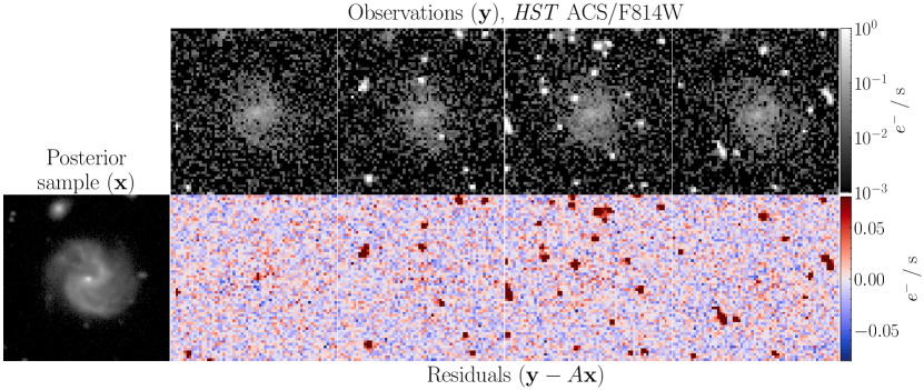
Figure 1: An example of a posterior sample for a COSMOS [7] target located at ${\mathrm{R.A.}=9^{\mathrm{h}}57^{\mathrm{m}}56^{\mathrm{s}}.5294}$, ${\mathrm{Dec.}=2^{\circ}27^{\prime}37^{\prime\prime}.963}$. The top row shows the 4 exposures jointly used in the likelihood. The bottom row shows a posterior sample (left) and the corresponding residuals (observation minus posterior sample) for this model.

2 Bayesian inference of galaxy surface brightness blurred with a PSF and in the presence of non-Gaussian noise

Our goal is to infer the posterior distribution of the surface brightness of galaxies on a pixelated grid. We denote the model galaxy images with $\mathbf{x}\in\mathbb{R}^{n}$, where $n$ is the number of pixels in the reconstructions, and the noisy telescope data with $\mathbf{y}\in\mathbb{R}^{m}$, where $m$ is the number of data pixels. The data-generating process can be written as

$$\mathbf{y}=A\mathbf{x}+\bm{\eta}\,.$$ (1)

where, $A\in\mathbb{R}^{m\times n}$ captures the telescope’s response process, including the blurring by the aperture — also known as the PSF — and wavefront aberrations from the optics. In this equation, $\bm{\eta}\in\mathbb{R}^{m}$ is a vector of additive noise, which captures the contribution of all additive stochastic phenomena other than the signal of interest to the data (e.g., CCD thermal noise, readout noise, cosmic rays, even astrophysical foreground/backgrounds, etc.). Since the noise is assumed to be additive, the likelihood can be written from the noise distribution directly: $\mathbf{y}-A\mathbf{x}\sim p(\bm{\eta})=p(\mathbf{y}\mid\mathbf{x})$.

The posterior distribution over $\mathbf{x}$ (model galaxy images) is proportionately given through Bayes’ theorem as the product of the prior $p(\mathbf{x})$ and the likelihood $p(\mathbf{y}\mid\mathbf{x})$

$$p(\mathbf{x}\mid\mathbf{y})\propto p(\mathbf{y}\mid\mathbf{x})p(\mathbf{x})\,.$$ (2)

An accurate characterization of the prior over the underconstrained variable $\mathbf{x}$ is crucial for this inference, as highlighted in numerous studies [37, 21, 38, 39, 40]. However, understanding the telescope noise distribution, $p(\bm{\eta})$, is of paramount importance to enable unbiased inference on real data. In the following section, we briefly overview the methodology employed to use data samples to learn both distributions — the prior and the likelihood — and combine them in order to sample from a close approximation to the posterior.

2.1 Prior and likelihood score-based modelling with Stochastic Differential Equations (SDE)

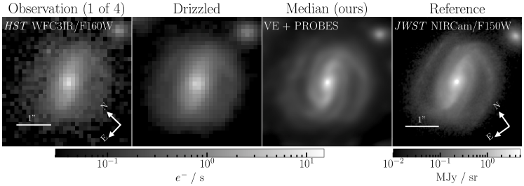
Figure 2: In the leftmost column, we show one of the HST exposures in the F160W filter for the target located at ${\mathrm{R.A.}=7^{\mathrm{h}}23^{\mathrm{m}}20^{\mathrm{s}}.7483}$; ${\mathrm{Dec.}=-73^{\circ}26^{\prime}07^{\prime\prime}.203}$ in the SMACS 0723 field used to obtain the drizzled image (second column) and the median image composed of $450$ posterior samples using our method (third column). In the rightmost column, we show the corresponding JWST image in the closest available filter to HST’s F160W filter as a reference. Note that neither the JWST image nor the drizzled image were used to perform the inference.

We make use of the continuous-time denoising score matching [41, 42, 43] framework developed in Song et al. [34] in order to learn the score of the prior, $\gradient_{\mathbf{x}}\log p(\mathbf{x})$, and the score of the noise distribution $\gradient_{\bm{\eta}}\log p(\bm{\eta})$. In summary, the objective function minimizes a weighted sum of Fisher divergences between the output of a neural network with a U-net architecture [44] and the score of a Gaussian perturbation kernel, $p(\mathbf{x}_{t}\mid\mathbf{x}_{0})=\mathcal{N}(\mathbf{x}_{t}\mid\mu(t)\mathbf{x}_{0},\sigma^{2}(t)\text{1}_{n\times n})$, both parameterized by the time variable $t\in[0,1]$ of an SDE. Within this framework, different choices of functions for $\mu(t)$ and $\sigma(t)$ can yield different properties on the generative model [see e.g. 45, 46]. Though any reasonable choice is in principle equivalent, they may differ in numerical stability. In this work, we focus on the well known Variance Exploding (VE) and Variance Preserving (VP) SDEs.

The strength of the aforementioned framework lies in the simplicity of the perturbation kernel. Assuming that $\mathbf{x}_{0}$ is a sample from the $t=0$ prior (the distribution of interest: $p(\mathbf{x}_{0})$) a sample from the SDE integrated up to time $t$ can be obtained directly from $p(\mathbf{x}_{t}\mid\mathbf{x}_{0})$. This simplicity also allows us to deduce the form of the perturbation kernel for the noise distribution, $p(\bm{\eta}_{t}\mid\bm{\eta}_{0})$, aimed at the posterior sampling SDE. Assuming $\mathbf{x}_{0}$ to be a sample from the posterior, we can use equation (1) and the prior perturbation kernel to obtain $\bm{\eta}_{t}=\mu(t)\bm{\eta}_{0}-A\sigma(t)\mathbf{z},$ where $\mathbf{z}\sim\mathcal{N}(0,\text{1}_{n\times n})$ and $\bm{\eta}_{0}=\mathbf{y}-A\mathbf{x}_{0}$. From this equation, we obtain a modified perturbation kernel that accounts for the Brownian motion injected through the physical model, $A$, when solving the posterior SDE:

$$p(\bm{\eta}_{t}\mid\bm{\eta}_{0})=\mathcal{N}(\mu(t)\bm{\eta}_{0},\sigma^{2}(t)AA^{T})$$ (3)

The score of the noise distribution, $\gradient_{\bm{\eta}_{t}}\log p_{t}(\bm{\eta}_{t})$, is thus constructed to have more accurate time marginals for the posterior SDE obtained by applying Anderson’s reverse-time formula [47] to the prior SDE and setting the posterior as the $t=0$ boundary condition of the SDE.

Following the work of Legin et al. [36], we can recover the likelihood score from the score of the noise distribution by applying the chain rule and using equation (1)

$$\gradient_{\mathbf{x}_{t}}\log p_{t}(\mathbf{y}\mid\mathbf{x}_{t})\approx-\gradient_{\bm{\eta}_{t}}\log p_{t}(\bm{\eta}_{t})A\,.$$ (4)

However, for time $t\not=0$, the above equation is an approximation to the true intractable likelihood score [38, 39, 40, 48], at $t=0$ it is exact. Our approximation relies on the assumption that the likelihood is much more informative than the prior [19, 21]. More details are provided in Appendix A.

2.2 Data and Physical Model

The PROBES dataset is a compendium of high-quality local late-type galaxies [49, 50] that we leverage to learn a prior from empirical observations of galaxies. These galaxies have resolved structures (bars, spiral arms, molecular clouds, etc.), which make them well suited to approximate what a high-resolution galaxy light profile looks like. This dataset has also been used in previous studies to train diffusion models [35, 21]. The SKIRT TNG [51] dataset is a large public collection of images spanning $0.3$-$5$ microns made by applying dust radiative transfer post-processing [52] to galaxies from the TNG cosmological magneto-hydrodynamical simulations [53] over redshifts $0.1\leq z\leq 0.7$. While this dataset inherits the assumptions about cosmology and the sub-grid physics that govern the formation of galactic structure in TNG [54, 55], it offers a unique opportunity to build our prior knowledge about the morphology of faint galaxies without interlopers, noise, and measurement effects inherent in the observed PROBES galaxies. In this work, we make use of the available $g$ and $z$ bands in both datasets to train the prior for optical (F814W) and near infrared (F160W) observations respectively.

The physical model is built with PyTorch [56] for its automatic differentiation capability. We incorporate 2 main components in the forward model, namely HST’s optical geometric distortions and the PSF. Geometrical distortions are represented through fourth-order polynomial transformations of pixel-to-world coordinates [57]. In practice, distorted world coordinates are extracted from the FITS files [58] of each observation using WCS routines from Astropy [59, 60, 61]. A bilinear interpolation is then applied between the model pixel coordinates and the observation world coordinates, similar to what is accomplished with the Drizzle algorithm [62] except without stacking the images. For the PSF, we make use of PyTorch’s 2D convolution algorithm and a public library of 4 times super-sampled PSF models for HST [63, 64]. Finally, the model resolution is set to match the observation resolution with the average pooling of the pixel values.

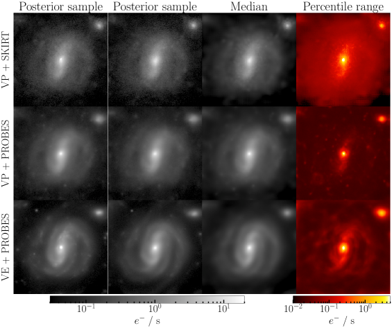
Figure 3: Comparison of the posterior samples, median and percentile range, defined as the $84\%-16\%$ range, for different SDE hyperparameters and prior for the same target as shown in Figure 2. Although the general shape of the image is recovered across the different hyperparameters, our method is able to recover more details using the VE SDE and the PROBES prior.

The observations used in this work are taken from two HST deep sky fields. Three observations of faint galaxies were selected from the COSMOS survey [7] and three additional targets are in the SMACS 0723 field. The SMACS 0723 targets offer the unique opportunity to compare our reconstructions from HST images with corresponding JWST images that are both much deeper and higher resolution. In this sense, the JWST images serve as ground truth for the techniques we deploy in this work. For each target, we gather all four dithered exposures captured within a single orbit of the HST from the Minkulsky Archive for Space Telescope. More specifically, we use the flat-fielded product from the HST pre-processing pipeline. We then multiply each exposure by the pixel area map and subtract the sky background. Our inference is performed jointly over all the exposures.

Finally, to train the score models over samples of the noise distributions, we take random cutouts from the full HST exposure for each target based on a flux cut. For the COSMOS targets, we collected 39,254 noise cutouts of shape $64\times 64$ pixels with a flux $F<0.02\,e^{-1}/s$. For the SMACS 0723 targets, we collected 8,747 noise cutouts of shape $32\times 32$ pixels with a flux $F<0.01\,e^{-1}/s$. For training, we approximate the physical model, $A$, with a circulant matrix in order to compute the perturbation kernel (3) efficiently with a Fast Fourier Transform (FFT) [65]. More details are provided in Appendix B.

3 Results and Discussion

As a test that our method can reliably produce samples even in the presence of cosmic rays, we show a reconstructed surface brightness profile in Figure 1 at a much higher resolution and depth than HST can give us for the F814W filter. Furthermore, the residuals in Figure 1 are plausible noise realizations from the telescope noise distribution, showing that all or nearly all of the galaxy surface brightness has been recovered. This is of high value for many morphological studies, which can run automated software on the posterior samples rather than the noisy data. Having access to posterior samples allows one to naturally propagate their uncertainties from the pixel flux measurements to the product of interest.

We validate that our method does not “hallucinate” morphologies by comparing posterior samples obtained from one of the SMACS 0723 targets with a deeper image of the same target from JWST in Figure 2. Note that the JWST image is only shown for reference and was never used during the inference. We also perform reconstructions using different combinations of SDEs and priors. We thus illustrate how different hyperparameter choices can impact the reconstructions, but also showcase how easy it is to swap in a different prior (potentially encoding different underlying assumptions) for a reconstruction. In principle, the likelihood function can also be easily modified, though should necessarily be tied to the instrument noise statistics. As can be seen, important morphological details are recovered in the posterior samples and median which are blurred or buried in noise in the HST observation shown in the upper left panel. In particular, the skewed bar feature is recovered, which was mostly blurred out in the HST observation. The spiral arms are also distinctly recovered. The core, however, is not strictly the same as JWST, using either of our priors. Posterior samples of additional targets are presented in Appendix C.

In summary, this work develops a framework for the Bayesian inference of surface brightness of galaxies in the presence of blurring by PSF and non-Gaussian additive noise, allowing maximal extraction of information from noisy data, with a high impact on numerous studies. The results of the method are validated using new higher-quality observations.

4 Acknowledgements

This research was made possible by a generous donation by Eric and Wendy Schmidt with the recommendation of the Schmidt Futures Foundation. We are also grateful to Nikolay Malkin for helpful discussions at various points of this project. The work is in part supported by computational resources provided by Calcul Quebec and the Digital Research Alliance of Canada. C.S. acknowledges support from the Natural Sciences and Engineering Council of Canada (NSERC) and the Canadian Institute for Theoretical Astrophysics (CITA). Y.H. and L.P. acknowledge support from the Natural Sciences and Engineering Council of Canada grant RGPIN-2020-05073 and 05102, the Fonds de recherche du Québec grant 2022-NC-301305 and 300397, and the Canada Research Chairs Program. The work of A.A. and R.L. were partially funded by NSERC CGS D scholarships. R.L. acknowledges support from the Centre for Research in Astrophysics of Quebec and the hospitality of the Flatiron Institute.

Some/all of the data presented in this paper were obtained from the Mikulski Archive for Space Telescopes (MAST). STScI is operated by the Association of Universities for Research in Astronomy, Inc., under NASA contract NAS5-26555.

Software used: astropy [59, 60], jupyter [66], matplotlib [67] , numpy [68], PyTorch [56], tqdm [69], pandas [70]

Appendix A Background on continuous-time score-matching and the convolved likelihood approximation

In this appendix, we provide some context to our methods, in particular, equation (3) and equation (4). We first give an overview of the continuous-time score-matching framework used to learn the score of the prior, $\gradient_{\mathbf{x}_{t}}\log p_{t}(\mathbf{x}_{t})$, from samples. We will then adapt this framework in order to construct an approximation to the likelihood score, $\gradient_{\mathbf{x}_{t}}\log p_{t}(\mathbf{y}\mid\mathbf{x}_{t})$, at every time $t\in[0,1]$ of the posterior sampling SDE. In the following, we will work with stochastic processes defined on a measurable space $(\mathbb{R}^{n},\mathcal{B}(\mathbb{R}^{n}),\{\mathcal{F}_{t}\},\mathbf{W})$ where $\mathcal{B}(\mathbb{R}^{n})$ is the Borel $\sigma$-algebra associated with $\mathbb{R}^{n}$, $\{\mathcal{F}_{t}\}$ is a set of filtrations and $\mathbf{W}$ is the Wiener measure.

A.1 Learning the prior

In order to construct a generative model for the prior, $p(\mathbf{x}_{0})$, where $\mathbf{x}_{0}\in\mathbb{R}^{n}$ can represent an image of a galaxy, we first construct a perturbation kernel, $p(\mathbf{x}_{t}\mid\mathbf{x}_{0})$, that progressively destroys all the information in available samples from the prior. Common choices for this perturbation kernel apply a stochastic process [34], $\mathbf{X}_{t}(\omega):[0,1]\times\Omega\rightarrow\mathbb{R}^{n}$, with a dynamic described by an SDE, $d\mathbf{x}=f(\mathbf{x},t)dt+g(t)d\mathbf{w}$, where $f$ is the drift, $g$ is an homogeneous diffusion coefficient and $\mathbf{w}$ is a Wiener process. In this work, we consider the Gaussian perturbation kernel for the Variance-Preserving (VP) or the Variance-Exploding (VE) SDE

$$p(\mathbf{x}_{t}\mid\mathbf{x}_{0})=\mathcal{N}(\mathbf{x}_{t}\mid\mu(t)\mathbf{x}_{0},\sigma^{2}(t)\text{1}_{n\times n})\,.$$ (5)

The perturbation kernel is used to train a neural network $\mathbf{s}_{\theta}(\mathbf{x},t):\mathbb{R}^{n}\times[0,1]\rightarrow\mathbb{R}^{n}$ to approximate the score of the prior, $\gradient_{\mathbf{x}_{t}}\log p(\mathbf{x}_{t})$, with a weighted sum of (forward) Fisher divergences as training objective:

$$\mathcal{L}_{\theta}=\mathbb{E}_{t\sim\mathcal{U}(0,1)}\mathbb{E}_{\mathbf{x}_{0}\sim p(\mathbf{x}_{0})}\mathbb{E}_{\mathbf{x}_{t}\sim p(\mathbf{x}_{t}\mid\mathbf{x}_{0})}\bigg{[}\lambda(t)\big{\lVert}\mathbf{s}_{\theta}(\mathbf{x}_{t},t)-\gradient_{\mathbf{x}_{t}}\log p(\mathbf{x}_{t}\mid\mathbf{x}_{0})\big{\rVert}_{2}^{2}\bigg{]}\,.$$ (6)

$\lambda(t)$ is a time-dependent weight factor chosen to be equal to the variance of the perturbation kernel, $\lambda(t)\equiv\sigma^{2}(t)$. See Song et al. [71] for a more general derivation of the loss. Since the perturbation kernel (5) is Gaussian, we can readily evaluate its score using the reparametrization

$$\mathbf{x}_{t}=\mu(t)\mathbf{x}_{0}+\sigma(t)\mathbf{z}\,,$$ (7)

where $\mathbf{z}\sim\mathcal{N}(0,\text{1}_{n\times n})$, such that we can write $\gradient_{\mathbf{x}_{t}}\log p_{t}(\mathbf{x}_{t}\mid\mathbf{x}_{0})=-\frac{\mathbf{z}}{\sigma(t)}$. The objective (6) is often written directly in terms of $\pm\mathbf{z}$, which highlights its connection with the denoising autoencoder objective [72].

A.2 The convolved likelihood approximation

The generative model for the prior is constructed by reversing time in the SDE using Anderson’s formula [47]. In order to sample from the posterior, we must change the $t=0$ boundary condition of the SDE to be the posterior distribution, $p(\mathbf{x}_{0}\mid\mathbf{y})$, instead of the prior, which yields the posterior sampling SDE

$$d\mathbf{x}=(f(\mathbf{x},t)-g^{2}(t)\gradient_{\mathbf{x}}\log p_{t}(\mathbf{x}\mid\mathbf{y}))dt+g(t)d\bar{\mathbf{w}}\,,$$ (8)

where $\bar{\mathbf{w}}$ is a time-reversed Wiener process. By applying Bayes’ theorem, we can make use of the score of the prior directly in the posterior sampling SDE without having to retrain or condition the model, $\mathbf{s}_{\theta}$, on the observation, $\mathbf{y}$:

$$\gradient_{\mathbf{x}_{t}}\log p_{t}(\mathbf{x}_{t}\mid\mathbf{y})=\gradient_{\mathbf{x}_{t}}\log p_{t}(\mathbf{y}\mid\mathbf{x}_{t})+\underbrace{\gradient_{\mathbf{x}_{t}}\log p_{t}(\mathbf{x}_{t})}_{\mathbf{s}_{\theta}(\mathbf{x}_{t},t)}\,.$$ (9)

Unfortunately, the likelihood in equation (9) is an intractable quantity to compute since it involves an expectation over $p(\mathbf{x}_{0}\mid\mathbf{x}_{t})$ of the likelihood at time $t=0$

$$p_{t}(\mathbf{y}\mid\mathbf{x}_{t})=\int d\mathbf{x}_{0}\,p(\mathbf{y}\mid\mathbf{x}_{0})p(\mathbf{x}_{0}\mid\mathbf{x}_{t})\,.$$ (10)

To simplify this expression, we reverse the conditional $p(\mathbf{x}_{0}\mid\mathbf{x}_{t})$ using Bayes’ theorem to get the known perturbation kernel of the SDE

$$p_{t}(\mathbf{y}\mid\mathbf{x}_{t})=\int d\mathbf{x}_{0}\,p(\mathbf{y}\mid\mathbf{x}_{0})p(\mathbf{x}_{t}\mid\mathbf{x}_{0})\frac{p(\mathbf{x}_{0})}{p_{t}(\mathbf{x}_{t})}\,.$$ (11)

The convolved likelihood approximation consists of taking the ratio $p(\mathbf{x}_{0})/p(\mathbf{x}_{t})$ to be a constant equal to 1. By ignoring this ratio, the integral becomes a convolution that is tractable, as we will show in the next subsection. However, this approximation means that we may introduce some bias in our posterior sampling method. We leave it to future work to explore better approximations and their trade-offs, as done e.g., in Feng et al. [39], Feng and Bouman [40] or Rozet and Louppe [48].

A.3 Learning the likelihood

We can now construct the perturbation kernel of the noise distribution, ${p(\bm{\eta}_{t}\mid\bm{\eta}_{0})}$, where $\bm{\eta}_{0}\in\mathbb{R}^{m}$ is the additive noise corrupting the observation $\mathbf{y}$ in equation (1). We multiply by $\mu(t)$ the data generating process, equation (1), and use the reparametrization of $\mathbf{x}_{t}$ in equation (7) to obtain

$$\mu(t)\mathbf{y} =A\mu(t)\mathbf{x}_{0}+\mu(t)\bm{\eta}_{0}$$

$$\implies\bm{\eta}_{t} =\mu(t)\bm{\eta}_{0}-A\sigma(t)\mathbf{z}\,.$$ (12)

We defined $\bm{\eta}_{t}\equiv\mu(t)\mathbf{y}-A\mathbf{x}_{t}$, the residuals of the model at time-index $t$ of the posterior SDE. This derivation relies on two crucial assumptions, namely that the physical model, $A\in\mathbb{R}^{m\times n}$, is linear, and that the noise in the inverse problem is additive. It is also worth noting that the equality $\bm{\eta}_{t}=\mu(t)\mathbf{y}-A\mathbf{x}_{t}$ can be used to infer $\bm{\eta}_{t}$ from the model $\mathbf{x}_{t}$ when solving the posterior SDE.

We can obtain the distribution of $\bm{\eta}_{t}$ from the RHS of equation (12). The addition of two random variables results in the convolution of their probability distribution, such that

$$p_{t}(\bm{\eta}_{t})=\int d\bm{\eta}_{0}\,p(\bm{\eta}_{0})p(\bm{\eta}_{t}\mid\bm{\eta}_{0})\,.$$ (13)

Equation (13) is the convolved likelihood approximation of equation (11). We define the perturbation kernel, $p(\bm{\eta}_{t}\mid\bm{\eta}_{0})$, as

$$p(\bm{\eta}_{t}\mid\bm{\eta}_{0})=p(\bm{\eta}_{t}-\mu(t)\bm{\eta}_{0})=p(-A\sigma(t)\mathbf{z})$$

Since $\mathbf{z}\sim\mathcal{N}(0,\text{1}_{n\times n})$, we obtain the distribution for the random variable $-A\sigma(t)\mathbf{z}$ by rescaling the covariance of the Gaussian distribution appropriately. Therefore,

$$p(\bm{\eta}_{t}\mid\bm{\eta}_{0})=\mathcal{N}(\bm{\eta}_{t}\mid\mu(t)\bm{\eta}_{0},\sigma^{2}(t)AA^{T})\,.$$ (14)

By using this perturbation kernel in the score-matching objective (6), we are able to train a neural network, $s_{\phi}(\bm{\eta},t):\mathbb{R}^{m}\times[0,1]\rightarrow\mathbb{R}^{m}$, which can be used to approximate the likelihood in the posterior sampling SDE. We obtain equation (4) by applying the chain rule to the approximate likelihood in equation (13) following the work of Legin et al. [36]

$$\gradient_{\mathbf{x}_{t}}\log p(\mathbf{y}\mid\mathbf{x}_{t})\approx\gradient_{\mathbf{x}_{t}}\log p_{t}(\bm{\eta}_{t})=-\underbrace{\gradient_{\bm{\eta}_{t}}\log p_{t}(\bm{\eta}_{t})}_{\mathbf{s}_{\phi}(\bm{\eta}_{t},t)}A\,.$$

In practice, and since we work in high dimensional spaces ($m,n\gtrsim 10^{4}$), we implement the formula above, also equation (4), known as Score-based Likelihood Characterisation (SLIC) [36], with the Vector-Jacobian Product (VJP). To do this, we implement the physical model, $A$, with Pytorch functions instead of using an explicit dense matrix. This strategy trades memory for compute in our sampling algorithm. A sketched implementation is shown in Figure 4.

⬇

import torch

from torch.func import vjp

\pardef slic_likelihood(y, x, t):

y_hat, vjp_func = vjp(A, x) # A is a callable function

eta = mu(t) * y - y_hat # residuals

score = s_phi(eta, t) # neural network

return -vjp_func(score)[0]

Figure 4: Sketched implementation of the SLIC likelihood with the Vector-Jacobian Product (VJP) operation using PyTorch [56].

Appendix B Circulant physical model approximation for the noise perturbation kernel

Similarly to the perturbation kernel of the prior, equation (5), we can evaluate the score of the noise perturbation kernel analytically, reparametrized in terms of the random variable $\mathbf{z}\in\mathbb{R}^{n}$, using equation (12)

$$\gradient_{\bm{\eta}_{t}}\log p(\bm{\eta}_{t}\mid\bm{\eta})=-\frac{1}{\sigma(t)}A\mathbf{z}(AA^{T})^{-1}\,.$$ (15)

To be evaluated numerically, the matrix $AA^{T}\in\mathrm{R}^{m\times m}$ needs to be invertible. In other words, it cannot have null eigenvalues. To ensure this, we add a small number to the diagonal of the matrix $A$. In this work, we add $\lambda=10^{-3}$.

In order to speed up the training of the noise score models, we approximate the physical model with a circulant matrix. By definition, a circulant matrix is a Toeplitz matrix, but each row is constructed from the same vector with its element cyclically permuted. If $A$ would only account for the point spread function, our approximation would be exact. Instead, $A\in\mathrm{R}^{m\times n}$ accounts for different transformations, including the different resolution of the model and the observation, which means $A$ is not strictly circulant and is a rectangular matrix with $m<n$. Our approximation for training the noise model consists of constructing a circulant matrix from the effective kernel of the physical model

$$A\approx\mathcal{F}^{\dagger}(\mathcal{F}\Pi_{k})\mathcal{F}\,,$$ (16)

where we define the effective kernel, $\Pi_{k}$, as the k^th column of $A$. With this technique, we remove some (but not all) of the null eigenvalues, assuming that most of the energy of the PSF is concentrated within a few pixels. In practice, we extract the column corresponding to the central pixel, $k=m^{2}/2$, from the physical model by making use of the Jacobian-Vector Product. We sketch an implementation in Figure 5.

With these two approximations, we can evaluate the score of the noise perturbation kernel in linear time using the Fast Fourier Transform [65]. We denote the unitary Fourier transform with $\mathcal{F}$ and the Hermitian conjugate with $\dagger$, such that

$$\gradient_{\bm{\eta}_{t}}p(\bm{\eta}_{t}\mid\bm{\eta}_{0})=-\frac{1}{\sigma(t)}\mathcal{F}^{\dagger}\mathcal{F}A\mathbf{z}(\mathcal{F}\Pi_{k})^{-2}\,.$$ (17)

This last equation is fast to evaluate since $\mathcal{F}\Pi_{k}$ is a diagonal matrix in Fourier space. We sketch its implementation in Figure 6.

⬇

from torch.func import jvp

\pardef effective_kernel(A, k):

x = torch.randn(n) # Random input for A

v = torch.zeros(n) # vector for the JVP

v[k] = 1. # Select column k

return jvp(A, (x,), (v,))[1]

Figure 5: Extraction of the column of the linear model implemented as a Pytorch function with the JVP.

⬇

power_spectrum = torch.fft.fft2(effective_kernel(A, k)).abs()**2 + 1e-3

def perturbation_kernel_score(z, t): # z is the a noise vector in R^n

y = torch.fft.fft2(A(z)) # A is the physical model

score_tilde = y / power_spectrum

return -torch.fft.ifft2(score_tilde).real / sigma(t)

Figure 6: Score of the perturbation kernel computed in linear time.

Appendix C Additional Figures

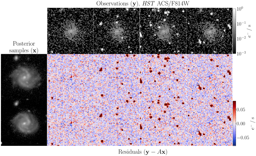
Figure 7: An example of two posterior samples for a COSMOS [7] target located at ${\mathrm{R.A.}=9^{\mathrm{h}}57^{\mathrm{m}}56^{\mathrm{s}}.5294}$, ${\mathrm{Dec.}=2^{\circ}27^{\prime}37^{\prime\prime}.963}$. The top row shows the 4 exposures jointly used in the likelihood. The middle and bottom rows show two posterior samples and their corresponding residuals against the observation.

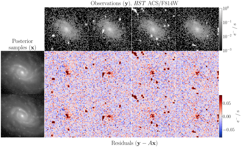
Figure 8: An example of two posterior samples for a COSMOS [7] target located at ${\mathrm{R.A.}=9^{\mathrm{h}}57^{\mathrm{m}}46^{\mathrm{s}}.8867}$, ${\mathrm{Dec.}=2^{\circ}28^{\prime}22^{\prime\prime}.735}$. The top row shows the 4 exposures jointly used in the likelihood. The middle and bottom rows show two posterior samples and their corresponding residuals against the observation.

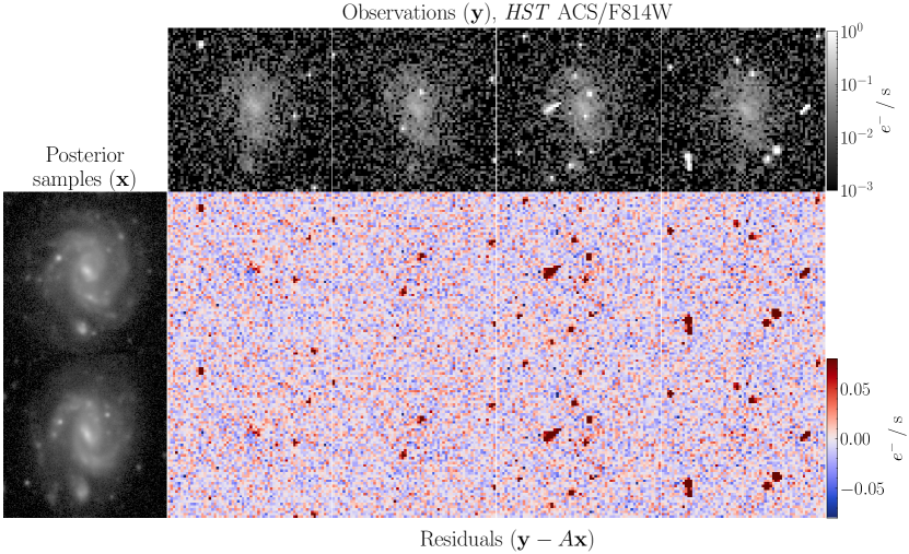
Figure 9: An example of two posterior samples for a COSMOS [7] target located at ${\mathrm{R.A.}=9^{\mathrm{h}}57^{\mathrm{m}}49^{\mathrm{s}}.1102}$, ${\mathrm{Dec.}=2^{\circ}28^{\prime}19^{\prime\prime}.430}$. The top row shows the 4 exposures jointly used in the likelihood. The middle and bottom rows show two posterior samples and their corresponding residuals against the observation.

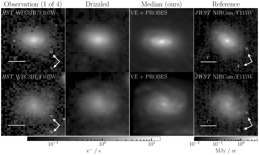
Figure 10: In the first row, leftmost column, we show one of the HST exposures in the F105W filter for the target located at ${\mathrm{R.A.}=7^{\mathrm{h}}23^{\mathrm{m}}24^{\mathrm{s}}.5462}$; ${\mathrm{Dec.}=-73^{\circ}27^{\prime}20^{\prime\prime}.172}$ in the SMACS 0723 field used to obtain the drizzled image (second column) and the median image composed of $450$ posterior samples using our method (third column). In the rightmost column, we show the corresponding JWST image in the closest available filter to HST F105W filter as a reference. Note that neither the JWST image nor the drizzled image were used to perform the inference. The second row reports the corresponding results for the target located at ${\mathrm{R.A.}=7^{\mathrm{h}}23^{\mathrm{m}}22^{\mathrm{s}}.0805}$; ${\mathrm{Dec.}=-73^{\circ}27^{\prime}24^{\prime\prime}.575}$ in the SMACS 0723 field.

References

- Walmsley et al. [2022] Mike Walmsley, Chris Lintott, Tobias Géron, Sandor Kruk, Coleman Krawczyk, Kyle W. Willett, Steven Bamford, Lee S. Kelvin, Lucy Fortson, Yarin Gal, William Keel, Karen L. Masters, Vihang Mehta, Brooke D. Simmons, Rebecca Smethurst, Lewis Smith, Elisabeth M. Baeten, and Christine Macmillan. Galaxy Zoo DECaLS: Detailed visual morphology measurements from volunteers and deep learning for 314 000 galaxies. MNRAS, 509(3):3966–3988, January 2022. doi: 10.1093/mnras/stab2093.
- Williams et al. [1996] Robert E. Williams, Brett Blacker, Mark Dickinson, W. Van Dyke Dixon, Henry C. Ferguson, Andrew S. Fruchter, Mauro Giavalisco, Ronald L. Gilliland, Inge Heyer, Rocio Katsanis, Zolt Levay, Ray A. Lucas, Douglas B. McElroy, Larry Petro, Marc Postman, Hans-Martin Adorf, and Richard Hook. The Hubble Deep Field: Observations, Data Reduction, and Galaxy Photometry. AJ, 112:1335, October 1996. doi: 10.1086/118105.
- Ferguson et al. [2000] Henry C. Ferguson, Mark Dickinson, and Robert Williams. The Hubble Deep Fields. ARA&A, 38:667–715, January 2000. doi: 10.1146/annurev.astro.38.1.667.
- Giavalisco et al. [2004] M. Giavalisco, M. Dickinson, H. C. Ferguson, S. Ravindranath, C. Kretchmer, L. A. Moustakas, P. Madau, S. M. Fall, Jonathan P. Gardner, M. Livio, C. Papovich, A. Renzini, H. Spinrad, D. Stern, and A. Riess. The rest-frame ultraviolet luminosity density of star-forming galaxies at redshifts z ¿ 3.5*. The Astrophysical Journal, 600(2):L103, jan 2004. doi: 10.1086/381244. URL https://dx.doi.org/10.1086/381244.
- Beckwith et al. [2006] Steven V. W. Beckwith, Massimo Stiavelli, Anton M. Koekemoer, John A. R. Caldwell, Henry C. Ferguson, Richard Hook, Ray A. Lucas, Louis E. Bergeron, Michael Corbin, Shardha Jogee, Nino Panagia, Massimo Robberto, Patricia Royle, Rachel S. Somerville, and Megan Sosey. The Hubble Ultra Deep Field. AJ, 132(5):1729–1755, November 2006. doi: 10.1086/507302.
- Davis et al. [2007] M. Davis, P. Guhathakurta, N. P. Konidaris, J. A. Newman, M. L. N. Ashby, A. D. Biggs, P. Barmby, K. Bundy, S. C. Chapman, A. L. Coil, C. J. Conselice, M. C. Cooper, D. J. Croton, P. R. M. Eisenhardt, R. S. Ellis, S. M. Faber, T. Fang, G. G. Fazio, A. Georgakakis, B. F. Gerke, W. M. Goss, S. Gwyn, J. Harker, A. M. Hopkins, J. S. Huang, R. J. Ivison, S. A. Kassin, E. N. Kirby, A. M. Koekemoer, D. C. Koo, E. S. Laird, E. Le Floc’h, L. Lin, J. M. Lotz, P. J. Marshall, D. C. Martin, A. J. Metevier, L. A. Moustakas, K. Nandra, K. G. Noeske, C. Papovich, A. C. Phillips, R. M. Rich, G. H. Rieke, D. Rigopoulou, S. Salim, D. Schiminovich, L. Simard, I. Smail, T. A. Small, B. J. Weiner, C. N. A. Willmer, S. P. Willner, G. Wilson, E. L. Wright, and R. Yan. The All-Wavelength Extended Groth Strip International Survey (AEGIS) Data Sets. ApJ, 660(1):L1–L6, May 2007. doi: 10.1086/517931.
- Scoville et al. [2007] N. Scoville, H. Aussel, M. Brusa, P. Capak, C. M. Carollo, M. Elvis, M. Giavalisco, L. Guzzo, G. Hasinger, C. Impey, J.-P. Kneib, O. LeFevre, S. J. Lilly, B. Mobasher, A. Renzini, R. M. Rich, D. B. Sanders, E. Schinnerer, D. Schminovich, P. Shopbell, Y. Taniguchi, and N. D. Tyson. The cosmic evolution survey (cosmos): Overview*. The Astrophysical Journal Supplement Series, 172(1):1, sep 2007. doi: 10.1086/516585. URL https://dx.doi.org/10.1086/516585.
- Windhorst et al. [2011] Rogier A. Windhorst, Seth H. Cohen, Nimish P. Hathi, Patrick J. McCarthy, Jr. Ryan, Russell E., Haojing Yan, Ivan K. Baldry, Simon P. Driver, Jay A. Frogel, David T. Hill, Lee S. Kelvin, Anton M. Koekemoer, Matt Mechtley, Robert W. O’Connell, Aaron S. G. Robotham, Michael J. Rutkowski, Mark Seibert, Amber N. Straughn, Richard J. Tuffs, Bruce Balick, Howard E. Bond, Howard Bushouse, Daniela Calzetti, Mark Crockett, Michael J. Disney, Michael A. Dopita, Donald N. B. Hall, Jon A. Holtzman, Sugata Kaviraj, Randy A. Kimble, John W. MacKenty, Max Mutchler, Francesco Paresce, Abihit Saha, Joseph I. Silk, John T. Trauger, Alistair R. Walker, Bradley C. Whitmore, and Erick T. Young. The Hubble Space Telescope Wide Field Camera 3 Early Release Science Data: Panchromatic Faint Object Counts for 0.2-2 m Wavelength. ApJS, 193(2):27, April 2011. doi: 10.1088/0067-0049/193/2/27.
- Grogin et al. [2011] Norman A. Grogin, Dale D. Kocevski, S. M. Faber, Henry C. Ferguson, Anton M. Koekemoer, Adam G. Riess, Viviana Acquaviva, David M. Alexander, Omar Almaini, Matthew L. N. Ashby, Marco Barden, Eric F. Bell, Frédéric Bournaud, Thomas M. Brown, Karina I. Caputi, Stefano Casertano, Paolo Cassata, Marco Castellano, Peter Challis, Ranga-Ram Chary, Edmond Cheung, Michele Cirasuolo, Christopher J. Conselice, Asantha Roshan Cooray, Darren J. Croton, Emanuele Daddi, Tomas Dahlen, Romeel Davé, Duília F. de Mello, Avishai Dekel, Mark Dickinson, Timothy Dolch, Jennifer L. Donley, James S. Dunlop, Aaron A. Dutton, David Elbaz, Giovanni G. Fazio, Alexei V. Filippenko, Steven L. Finkelstein, Adriano Fontana, Jonathan P. Gardner, Peter M. Garnavich, Eric Gawiser, Mauro Giavalisco, Andrea Grazian, Yicheng Guo, Nimish P. Hathi, Boris Häussler, Philip F. Hopkins, Jia-Sheng Huang, Kuang-Han Huang, Saurabh W. Jha, Jeyhan S. Kartaltepe, Robert P. Kirshner, David C. Koo, Kamson Lai, Kyoung-Soo Lee, Weidong Li, Jennifer M. Lotz, Ray A. Lucas, Piero Madau, Patrick J. McCarthy, Elizabeth J. McGrath, Daniel H. McIntosh, Ross J. McLure, Bahram Mobasher, Leonidas A. Moustakas, Mark Mozena, Kirpal Nandra, Jeffrey A. Newman, Sami-Matias Niemi, Kai G. Noeske, Casey J. Papovich, Laura Pentericci, Alexandra Pope, Joel R. Primack, Abhijith Rajan, Swara Ravindranath, Naveen A. Reddy, Alvio Renzini, Hans-Walter Rix, Aday R. Robaina, Steven A. Rodney, David J. Rosario, Piero Rosati, Sara Salimbeni, Claudia Scarlata, Brian Siana, Luc Simard, Joseph Smidt, Rachel S. Somerville, Hyron Spinrad, Amber N. Straughn, Louis-Gregory Strolger, Olivia Telford, Harry I. Teplitz, Jonathan R. Trump, Arjen van der Wel, Carolin Villforth, Risa H. Wechsler, Benjamin J. Weiner, Tommy Wiklind, Vivienne Wild, Grant Wilson, Stijn Wuyts, Hao-Jing Yan, and Min S. Yun. CANDELS: The Cosmic Assembly Near-infrared Deep Extragalactic Legacy Survey. ApJS, 197(2):35, December 2011. doi: 10.1088/0067-0049/197/2/35.
- Koekemoer et al. [2011] Anton M. Koekemoer, S. M. Faber, Henry C. Ferguson, Norman A. Grogin, Dale D. Kocevski, David C. Koo, Kamson Lai, Jennifer M. Lotz, Ray A. Lucas, Elizabeth J. McGrath, Sara Ogaz, Abhijith Rajan, Adam G. Riess, Steve A. Rodney, Louis Strolger, Stefano Casertano, Marco Castellano, Tomas Dahlen, Mark Dickinson, Timothy Dolch, Adriano Fontana, Mauro Giavalisco, Andrea Grazian, Yicheng Guo, Nimish P. Hathi, Kuang-Han Huang, Arjen van der Wel, Hao-Jing Yan, Viviana Acquaviva, David M. Alexander, Omar Almaini, Matthew L. N. Ashby, Marco Barden, Eric F. Bell, Frédéric Bournaud, Thomas M. Brown, Karina I. Caputi, Paolo Cassata, Peter J. Challis, Ranga-Ram Chary, Edmond Cheung, Michele Cirasuolo, Christopher J. Conselice, Asantha Roshan Cooray, Darren J. Croton, Emanuele Daddi, Romeel Davé, Duilia F. de Mello, Loic de Ravel, Avishai Dekel, Jennifer L. Donley, James S. Dunlop, Aaron A. Dutton, David Elbaz, Giovanni G. Fazio, Alexei V. Filippenko, Steven L. Finkelstein, Chris Frazer, Jonathan P. Gardner, Peter M. Garnavich, Eric Gawiser, Ruth Gruetzbauch, Will G. Hartley, Boris Häussler, Jessica Herrington, Philip F. Hopkins, Jia-Sheng Huang, Saurabh W. Jha, Andrew Johnson, Jeyhan S. Kartaltepe, Ali A. Khostovan, Robert P. Kirshner, Caterina Lani, Kyoung-Soo Lee, Weidong Li, Piero Madau, Patrick J. McCarthy, Daniel H. McIntosh, Ross J. McLure, Conor McPartland, Bahram Mobasher, Heidi Moreira, Alice Mortlock, Leonidas A. Moustakas, Mark Mozena, Kirpal Nandra, Jeffrey A. Newman, Jennifer L. Nielsen, Sami Niemi, Kai G. Noeske, Casey J. Papovich, Laura Pentericci, Alexandra Pope, Joel R. Primack, Swara Ravindranath, Naveen A. Reddy, Alvio Renzini, Hans-Walter Rix, Aday R. Robaina, David J. Rosario, Piero Rosati, Sara Salimbeni, Claudia Scarlata, Brian Siana, Luc Simard, Joseph Smidt, Diana Snyder, Rachel S. Somerville, Hyron Spinrad, Amber N. Straughn, Olivia Telford, Harry I. Teplitz, Jonathan R. Trump, Carlos Vargas, Carolin Villforth, Cory R. Wagner, Pat Wandro, Risa H. Wechsler, Benjamin J. Weiner, Tommy Wiklind, Vivienne Wild, Grant Wilson, Stijn Wuyts, and Min S. Yun. CANDELS: The Cosmic Assembly Near-infrared Deep Extragalactic Legacy Survey—The Hubble Space Telescope Observations, Imaging Data Products, and Mosaics. ApJS, 197(2):36, December 2011. doi: 10.1088/0067-0049/197/2/36.
- Brammer et al. [2012] Gabriel B. Brammer, Pieter G. van Dokkum, Marijn Franx, Mattia Fumagalli, Shannon Patel, Hans-Walter Rix, Rosalind E. Skelton, Mariska Kriek, Erica Nelson, Kasper B. Schmidt, Rachel Bezanson, Elisabete da Cunha, Dawn K. Erb, Xiaohui Fan, Natascha Förster Schreiber, Garth D. Illingworth, Ivo Labbé, Joel Leja, Britt Lundgren, Dan Magee, Danilo Marchesini, Patrick McCarthy, Ivelina Momcheva, Adam Muzzin, Ryan Quadri, Charles C. Steidel, Tomer Tal, David Wake, Katherine E. Whitaker, and Anna Williams. 3D-HST: A Wide-field Grism Spectroscopic Survey with the Hubble Space Telescope. ApJS, 200(2):13, June 2012. doi: 10.1088/0067-0049/200/2/13.
- Lotz et al. [2017] J. M. Lotz, A. Koekemoer, D. Coe, N. Grogin, P. Capak, J. Mack, J. Anderson, R. Avila, E. A. Barker, D. Borncamp, G. Brammer, M. Durbin, H. Gunning, B. Hilbert, H. Jenkner, H. Khandrika, Z. Levay, R. A. Lucas, J. MacKenty, S. Ogaz, B. Porterfield, N. Reid, M. Robberto, P. Royle, L. J. Smith, L. J. Storrie-Lombardi, B. Sunnquist, J. Surace, D. C. Taylor, R. Williams, J. Bullock, M. Dickinson, S. Finkelstein, P. Natarajan, J. Richard, B. Robertson, J. Tumlinson, A. Zitrin, K. Flanagan, K. Sembach, B. T. Soifer, and M. Mountain. The Frontier Fields: Survey Design and Initial Results. ApJ, 837(1):97, March 2017. doi: 10.3847/1538-4357/837/1/97.
- Conselice [2003] Christopher J. Conselice. The relationship between stellar light distributions of galaxies and their formation histories. The Astrophysical Journal Supplement Series, 147(1):1, jul 2003. doi: 10.1086/375001. URL https://dx.doi.org/10.1086/375001.
- van der Wel et al. [2014] A. van der Wel, M. Franx, P. G. van Dokkum, R. E. Skelton, I. G. Momcheva, K. E. Whitaker, G. B. Brammer, E. F. Bell, H. W. Rix, S. Wuyts, H. C. Ferguson, B. P. Holden, G. Barro, A. M. Koekemoer, Yu-Yen Chang, E. J. McGrath, B. Häussler, A. Dekel, P. Behroozi, M. Fumagalli, J. Leja, B. F. Lundgren, M. V. Maseda, E. J. Nelson, D. A. Wake, S. G. Patel, I. Labbé, S. M. Faber, N. A. Grogin, and D. D. Kocevski. 3D-HST+CANDELS: The Evolution of the Galaxy Size-Mass Distribution since z = 3. ApJ, 788(1):28, June 2014. doi: 10.1088/0004-637X/788/1/28.
- Tacchella et al. [2019] Sandro Tacchella, Benedikt Diemer, Lars Hernquist, Shy Genel, Federico Marinacci, Dylan Nelson, Annalisa Pillepich, Vicente Rodriguez-Gomez, Laura V Sales, Volker Springel, and Mark Vogelsberger. Morphology and star formation in IllustrisTNG: the build-up of spheroids and discs. Monthly Notices of the Royal Astronomical Society, 487(4):5416–5440, 06 2019. ISSN 0035-8711. doi: 10.1093/mnras/stz1657. URL https://doi.org/10.1093/mnras/stz1657.
- Bluck et al. [2019] Asa F. L. Bluck, Connor Bottrell, Hossen Teimoorinia, Bruno M. B. Henriques, J. Trevor Mendel, Sara L. Ellison, Karun Thanjavur, Luc Simard, David R. Patton, Christopher J. Conselice, Jorge Moreno, and Joanna Woo. What shapes a galaxy? - unraveling the role of mass, environment, and star formation in forming galactic structure. MNRAS, 485(1):666–696, May 2019. doi: 10.1093/mnras/stz363.
- Masters and Galaxy Zoo Team [2020] Karen L. Masters and Galaxy Zoo Team. Twelve years of Galaxy Zoo. In Monica Valluri and J. A. Sellwood, editors, Galactic Dynamics in the Era of Large Surveys, volume 353, pages 205–212, January 2020. doi: 10.1017/S1743921319008615.
- Starck et al. [2002] J. L. Starck, E. Pantin, and F. Murtagh. Deconvolution in Astronomy: A Review. PASP, 114(800):1051–1069, October 2002. doi: 10.1086/342606.
- Remy et al. [2022] Benjamin Remy, Francois Lanusse, Niall Jeffrey, Jia Liu, Jean-Luc Starck, Ken Osato, and Tim Schrabback. Probabilistic Mass Mapping with Neural Score Estimation. arXiv e-prints, art. arXiv:2201.05561, January 2022.
- Graikos et al. [2022] Alexandros Graikos, Nikolay Malkin, Nebojsa Jojic, and Dimitris Samaras. Diffusion models as plug-and-play priors. arXiv e-prints, art. arXiv:2206.09012, June 2022. doi: 10.48550/arXiv.2206.09012.
- Adam et al. [2022] Alexandre Adam, Adam Coogan, Nikolay Malkin, Ronan Legin, Laurence Perreault-Levasseur, Yashar Hezaveh, and Yoshua Bengio. Posterior samples of source galaxies in strong gravitational lenses with score-based priors. arXiv e-prints, art. arXiv:2211.03812, November 2022. doi: 10.48550/arXiv.2211.03812.
- Högbom [1974] J. A. Högbom. Aperture Synthesis with a Non-Regular Distribution of Interferometer Baselines. A&AS, 15:417, June 1974.
- Michalewicz et al. [2023] Kevin Michalewicz, Martin Millon, Frédéric Dux, and Frédéric Courbin. Starred: a two-channel deconvolution method with starlet regularization. Journal of Open Source Software, 8(85):5340, 2023. doi: 10.21105/joss.05340. URL https://doi.org/10.21105/joss.05340.
- Lucy [1994] L. B. Lucy. Image Restorations of High Photometric Quality. In Robert J. Hanisch and Richard L. White, editors, The Restoration of HST Images and Spectra - II, page 79, January 1994.
- Bertero et al. [1998] Mario Bertero, Patrizia Boccacci, and Massimo Robberto. Inversion method for the restoration of chopped and nodded images. In Albert M. Fowler, editor, Infrared Astronomical Instrumentation, volume 3354 of Society of Photo-Optical Instrumentation Engineers (SPIE) Conference Series, pages 877–886, August 1998. doi: 10.1117/12.317254.
- Dong et al. [2020] Jiangxin Dong, Stefan Roth, and Bernt Schiele. Deep wiener deconvolution: Wiener meets deep learning for image deblurring. In H. Larochelle, M. Ranzato, R. Hadsell, M.F. Balcan, and H. Lin, editors, Advances in Neural Information Processing Systems, volume 33, pages 1048–1059. Curran Associates, Inc., 2020. URL https://proceedings.neurips.cc/paper_files/paper/2020/file/0b8aff0438617c055eb55f0ba5d226fa-Paper.pdf.
- Akhaury et al. [2022] Utsav Akhaury, Jean-Luc Starck, Pascale Jablonka, Frédéric Courbin, and Kevin Michalewicz. Deep Learning-based galaxy image deconvolution. Frontiers in Astronomy and Space Sciences, 9:357, November 2022. doi: 10.3389/fspas.2022.1001043.
- Morningstar et al. [2018] Warren R. Morningstar, Yashar D. Hezaveh, Laurence Perreault Levasseur, Roger D. Blandford, Philip J. Marshall, Patrick Putzky, and Risa H. Wechsler. Analyzing interferometric observations of strong gravitational lenses with recurrent and convolutional neural networks. arXiv e-prints, art. arXiv:1808.00011, July 2018. doi: 10.48550/arXiv.1808.00011.
- Morningstar et al. [2019] Warren R. Morningstar, Laurence Perreault Levasseur, Yashar D. Hezaveh, Roger Blandford, Phil Marshall, Patrick Putzky, Thomas D. Rueter, Risa Wechsler, and Max Welling. Data-driven Reconstruction of Gravitationally Lensed Galaxies Using Recurrent Inference Machines. ApJ, 883(1):14, September 2019. doi: 10.3847/1538-4357/ab35d7.
- Adam et al. [2023] Alexandre Adam, Laurence Perreault-Levasseur, Yashar Hezaveh, and Max Welling. Pixelated Reconstruction of Foreground Density and Background Surface Brightness in Gravitational Lensing Systems Using Recurrent Inference Machines. ApJ, 951(1):6, July 2023. doi: 10.3847/1538-4357/accf84.
- Wang et al. [2023] Hong Wang, Sreevarsha Sreejith, Yuewei Lin, Nesar Ramachandra, Anže Solsar, and Shinjae Yoo. Neural Network Based Point Spread Function Deconvolution For Astronomical Applications. The Open Journal of Astrophysics, 6:30, August 2023. doi: 10.21105/astro.2210.01666.
- Stone et al. [2023] Connor J. Stone, Stéphane Courteau, Jean-Charles Cuillandre, Yashar Hezaveh, Laurence Perreault-Levasseur, and Nikhil Arora. AstroPhot: Fitting Everything Everywhere All at Once in Astronomical Images. MNRAS, August 2023. doi: 10.1093/mnras/stad2477.
- Ho et al. [2020] Jonathan Ho, Ajay Jain, and Pieter Abbeel. Denoising diffusion probabilistic models. 33:6840–6851, 2020. URL https://proceedings.neurips.cc/paper/2020/file/4c5bcfec8584af0d967f1ab10179ca4b-Paper.pdf.
- Song et al. [2020] Yang Song, Jascha Sohl-Dickstein, Diederik P. Kingma, Abhishek Kumar, Stefano Ermon, and Ben Poole. Score-Based Generative Modeling through Stochastic Differential Equations. arXiv e-prints, art. arXiv:2011.13456, November 2020. doi: 10.48550/arXiv.2011.13456.
- Smith et al. [2022] Michael J. Smith, James E. Geach, Ryan A. Jackson, Nikhil Arora, Connor Stone, and Stéphane Courteau. Realistic galaxy image simulation via score-based generative models. Monthly Notices of the Royal Astronomical Society, 511(2):1808–1818, April 2022. doi: 10.1093/mnras/stac130.
- Legin et al. [2023] Ronan Legin, Alexandre Adam, Yashar Hezaveh, and Laurence Perreault-Levasseur. Beyond gaussian noise: A generalized approach to likelihood analysis with non-gaussian noise. The Astrophysical Journal Letters, 949(2):L41, 2023.
- Song et al. [2021a] Yang Song, Liyue Shen, Lei Xing, and Stefano Ermon. Solving Inverse Problems in Medical Imaging with Score-Based Generative Models. arXiv e-prints, art. arXiv:2111.08005, November 2021a. doi: 10.48550/arXiv.2111.08005.
- Chung et al. [2022] Hyungjin Chung, Jeongsol Kim, Michael T. Mccann, Marc L. Klasky, and Jong Chul Ye. Diffusion Posterior Sampling for General Noisy Inverse Problems. arXiv e-prints, art. arXiv:2209.14687, September 2022. doi: 10.48550/arXiv.2209.14687.
- Feng et al. [2023] Berthy T. Feng, Jamie Smith, Michael Rubinstein, Huiwen Chang, Katherine L. Bouman, and William T. Freeman. Score-Based Diffusion Models as Principled Priors for Inverse Imaging. arXiv e-prints, art. arXiv:2304.11751, April 2023. doi: 10.48550/arXiv.2304.11751.
- Feng and Bouman [2023] Berthy T. Feng and Katherine L. Bouman. Efficient Bayesian Computational Imaging with a Surrogate Score-Based Prior. arXiv e-prints, art. arXiv:2309.01949, September 2023. doi: 10.48550/arXiv.2309.01949.
- Hyvärinen [2005] Aapo Hyvärinen. Estimation of non-normalized statistical models by score matching. Journal of Machine Learning Research, 6(24):695–709, 2005. URL http://jmlr.org/papers/v6/hyvarinen05a.html.
- Vincent [2011] Pascal Vincent. A connection between score matching and denoising autoencoders. Neural Comput., 23(7):1661–1674, 2011. doi: 10.1162/NECO“˙a“˙00142. URL https://doi.org/10.1162/NECO_a_00142.
- Alain and Bengio [2014] Guillaume Alain and Yoshua Bengio. What regularized auto-encoders learn from the data-generating distribution. J. Mach. Learn. Res., 15(1):3563–3593, jan 2014. ISSN 1532-4435.
- Ronneberger et al. [2015] Olaf Ronneberger, Philipp Fischer, and Thomas Brox. U-Net: Convolutional Networks for Biomedical Image Segmentation. arXiv e-prints, art. arXiv:1505.04597, May 2015. doi: 10.48550/arXiv.1505.04597.
- Song and Ermon [2020] Yang Song and Stefano Ermon. Improved techniques for training score-based generative models. CoRR, abs/2006.09011, 2020. URL https://arxiv.org/abs/2006.09011.
- Karras et al. [2022] Tero Karras, Miika Aittala, Timo Aila, and Samuli Laine. Elucidating the Design Space of Diffusion-Based Generative Models. arXiv e-prints, art. arXiv:2206.00364, June 2022. doi: 10.48550/arXiv.2206.00364.
- Anderson [1982] Brian D.O. Anderson. Reverse-time diffusion equation models. Stochastic Processes and their Applications, 12(3):313–326, 1982. ISSN 0304-4149. doi: https://doi.org/10.1016/0304-4149(82)90051-5. URL https://www.sciencedirect.com/science/article/pii/0304414982900515.
- Rozet and Louppe [2023] François Rozet and Gilles Louppe. Score-based Data Assimilation. arXiv e-prints, art. arXiv:2306.10574, June 2023. doi: 10.48550/arXiv.2306.10574.
- Stone and Courteau [2019] Connor Stone and Stéphane Courteau. The Intrinsic Scatter of the Radial Acceleration Relation. The Astrophysical Journal, 882(1):6, September 2019. doi: 10.3847/1538-4357/ab3126.
- Stone et al. [2021] Connor Stone, Stéphane Courteau, and Nikhil Arora. The Intrinsic Scatter of Galaxy Scaling Relations. The Astrophysical Journal, 912(1):41, May 2021. doi: 10.3847/1538-4357/abebe4.
- Bottrell et al. [2023] Connor Bottrell, Hassen M. Yesuf, Gergö Popping, Kiyoaki Christopher Omori, Shenli Tang, Xuheng Ding, Annalisa Pillepich, Dylan Nelson, Lukas Eisert, Hua Gao, Andy D. Goulding, Boris S. Kalita, Wentao Luo, Jenny E. Greene, Jingjing Shi, and John D. Silverman. IllustrisTNG in the HSC-SSP: image data release and the major role of mini mergers as drivers of asymmetry and star formation. arXiv e-prints, art. arXiv:2308.14793, August 2023. doi: 10.48550/arXiv.2308.14793.
- Camps and Baes [2020] P. Camps and M. Baes. Skirt 9: Redesigning an advanced dust radiative transfer code to allow kinematics, line transfer and polarization by aligned dust grains. Astronomy and Computing, 31:100381, 2020. ISSN 2213-1337. doi: https://doi.org/10.1016/j.ascom.2020.100381. URL https://www.sciencedirect.com/science/article/pii/S2213133720300354.
- Nelson et al. [2019] Dylan Nelson, Volker Springel, Annalisa Pillepich, Vicente Rodriguez-Gomez, Paul Torrey, Shy Genel, Mark Vogelsberger, Ruediger Pakmor, Federico Marinacci, Rainer Weinberger, Luke Kelley, Mark Lovell, Benedikt Diemer, and Lars Hernquist. The IllustrisTNG simulations: public data release. Computational Astrophysics and Cosmology, 6(1):2, May 2019. doi: 10.1186/s40668-019-0028-x.
- Weinberger et al. [2017] Rainer Weinberger, Volker Springel, Lars Hernquist, Annalisa Pillepich, Federico Marinacci, Rüdiger Pakmor, Dylan Nelson, Shy Genel, Mark Vogelsberger, Jill Naiman, and Paul Torrey. Simulating galaxy formation with black hole driven thermal and kinetic feedback. MNRAS, 465(3):3291–3308, Mar 2017. doi: 10.1093/mnras/stw2944.
- Pillepich et al. [2018] A. Pillepich, V. Springel, D. Nelson, S. Genel, J. Naiman, R. Pakmor, L. Hernquist, P. Torrey, M. Vogelsberger, R. Weinberger, and F. Marinacci. Simulating galaxy formation with the IllustrisTNG model. MNRAS, 473:4077–4106, January 2018. doi: 10.1093/mnras/stx2656.
- Paszke et al. [2019] Adam Paszke, Sam Gross, Francisco Massa, Adam Lerer, James Bradbury, Gregory Chanan, Trevor Killeen, Zeming Lin, Natalia Gimelshein, Luca Antiga, Alban Desmaison, Andreas Kopf, Edward Yang, Zachary DeVito, Martin Raison, Alykhan Tejani, Sasank Chilamkurthy, Benoit Steiner, Lu Fang, Junjie Bai, and Soumith Chintala. Pytorch: An imperative style, high-performance deep learning library. In H. Wallach, H. Larochelle, A. Beygelzimer, F. d'Alché-Buc, E. Fox, and R. Garnett, editors, Advances in Neural Information Processing Systems 32, pages 8024–8035. Curran Associates, Inc., 2019. URL http://papers.neurips.cc/paper/9015-pytorch-an-imperative-style-high-performance-deep-learning-library.pdf.
- Bellini and Bedin [2009] A. Bellini and L. R. Bedin. Astrometry and Photometry with HST WFC3. I. Geometric Distortion Corrections of F225W, F275W, F336W Bands of the UVIS Channel. PASP, 121(886):1419, December 2009. doi: 10.1086/649061.
- Pence et al. [2010] W. D. Pence, L. Chiappetti, C. G. Page, R. A. Shaw, and E. Stobie. Definition of the Flexible Image Transport System (FITS), version 3.0. A&A, 524:A42, December 2010. doi: 10.1051/0004-6361/201015362.
- Astropy Collaboration et al. [2013] Astropy Collaboration, T. P. Robitaille, E. J. Tollerud, P. Greenfield, M. Droettboom, E. Bray, T. Aldcroft, M. Davis, A. Ginsburg, A. M. Price-Whelan, W. E. Kerzendorf, A. Conley, N. Crighton, K. Barbary, D. Muna, H. Ferguson, F. Grollier, M. M. Parikh, P. H. Nair, H. M. Unther, C. Deil, J. Woillez, S. Conseil, R. Kramer, J. E. H. Turner, L. Singer, R. Fox, B. A. Weaver, V. Zabalza, Z. I. Edwards, K. Azalee Bostroem, D. J. Burke, A. R. Casey, S. M. Crawford, N. Dencheva, J. Ely, T. Jenness, K. Labrie, P. L. Lim, F. Pierfederici, A. Pontzen, A. Ptak, B. Refsdal, M. Servillat, and O. Streicher. Astropy: A community Python package for astronomy. Astronomy and Astrophysics, 558:A33, October 2013. doi: 10.1051/0004-6361/201322068.
- Astropy Collaboration et al. [2018] Astropy Collaboration, A. M. Price-Whelan, B. M. Sipőcz, H. M. Günther, P. L. Lim, S. M. Crawford, S. Conseil, D. L. Shupe, M. W. Craig, N. Dencheva, A. Ginsburg, J. T. Vand erPlas, L. D. Bradley, D. Pérez-Suárez, M. de Val-Borro, T. L. Aldcroft, K. L. Cruz, T. P. Robitaille, E. J. Tollerud, C. Ardelean, T. Babej, Y. P. Bach, M. Bachetti, A. V. Bakanov, S. P. Bamford, G. Barentsen, P. Barmby, A. Baumbach, K. L. Berry, F. Biscani, M. Boquien, K. A. Bostroem, L. G. Bouma, G. B. Brammer, E. M. Bray, H. Breytenbach, H. Buddelmeijer, D. J. Burke, G. Calderone, J. L. Cano Rodríguez, M. Cara, J. V. M. Cardoso, S. Cheedella, Y. Copin, L. Corrales, D. Crichton, D. D’Avella, C. Deil, É. Depagne, J. P. Dietrich, A. Donath, M. Droettboom, N. Earl, T. Erben, S. Fabbro, L. A. Ferreira, T. Finethy, R. T. Fox, L. H. Garrison, S. L. J. Gibbons, D. A. Goldstein, R. Gommers, J. P. Greco, P. Greenfield, A. M. Groener, F. Grollier, A. Hagen, P. Hirst, D. Homeier, A. J. Horton, G. Hosseinzadeh, L. Hu, J. S. Hunkeler, Ž. Ivezić, A. Jain, T. Jenness, G. Kanarek, S. Kendrew, N. S. Kern, W. E. Kerzendorf, A. Khvalko, J. King, D. Kirkby, A. M. Kulkarni, A. Kumar, A. Lee, D. Lenz, S. P. Littlefair, Z. Ma, D. M. Macleod, M. Mastropietro, C. McCully, S. Montagnac, B. M. Morris, M. Mueller, S. J. Mumford, D. Muna, N. A. Murphy, S. Nelson, G. H. Nguyen, J. P. Ninan, M. Nöthe, S. Ogaz, S. Oh, J. K. Parejko, N. Parley, S. Pascual, R. Patil, A. A. Patil, A. L. Plunkett, J. X. Prochaska, T. Rastogi, V. Reddy Janga, J. Sabater, P. Sakurikar, M. Seifert, L. E. Sherbert, H. Sherwood-Taylor, A. Y. Shih, J. Sick, M. T. Silbiger, S. Singanamalla, L. P. Singer, P. H. Sladen, K. A. Sooley, S. Sornarajah, O. Streicher, P. Teuben, S. W. Thomas, G. R. Tremblay, J. E. H. Turner, V. Terrón, M. H. van Kerkwijk, A. de la Vega, L. L. Watkins, B. A. Weaver, J. B. Whitmore, J. Woillez, V. Zabalza, and Astropy Contributors. The Astropy Project: Building an Open-science Project and Status of the v2.0 Core Package. Astronomical Journal, 156(3):123, September 2018. doi: 10.3847/1538-3881/aabc4f.
- Astropy Collaboration et al. [2022] Astropy Collaboration, Adrian M. Price-Whelan, Pey Lian Lim, Nicholas Earl, Nathaniel Starkman, Larry Bradley, David L. Shupe, Aarya A. Patil, Lia Corrales, C. E. Brasseur, Maximilian N”othe, Axel Donath, Erik Tollerud, Brett M. Morris, Adam Ginsburg, Eero Vaher, Benjamin A. Weaver, James Tocknell, William Jamieson, Marten H. van Kerkwijk, Thomas P. Robitaille, Bruce Merry, Matteo Bachetti, H. Moritz G”unther, Thomas L. Aldcroft, Jaime A. Alvarado-Montes, Anne M. Archibald, Attila B’odi, Shreyas Bapat, Geert Barentsen, Juanjo Baz’an, Manish Biswas, M’ed’eric Boquien, D. J. Burke, Daria Cara, Mihai Cara, Kyle E. Conroy, Simon Conseil, Matthew W. Craig, Robert M. Cross, Kelle L. Cruz, Francesco D’Eugenio, Nadia Dencheva, Hadrien A. R. Devillepoix, J”org P. Dietrich, Arthur Davis Eigenbrot, Thomas Erben, Leonardo Ferreira, Daniel Foreman-Mackey, Ryan Fox, Nabil Freij, Suyog Garg, Robel Geda, Lauren Glattly, Yash Gondhalekar, Karl D. Gordon, David Grant, Perry Greenfield, Austen M. Groener, Steve Guest, Sebastian Gurovich, Rasmus Handberg, Akeem Hart, Zac Hatfield-Dodds, Derek Homeier, Griffin Hosseinzadeh, Tim Jenness, Craig K. Jones, Prajwel Joseph, J. Bryce Kalmbach, Emir Karamehmetoglu, Mikolaj Kaluszy’nski, Michael S. P. Kelley, Nicholas Kern, Wolfgang E. Kerzendorf, Eric W. Koch, Shankar Kulumani, Antony Lee, Chun Ly, Zhiyuan Ma, Conor MacBride, Jakob M. Maljaars, Demitri Muna, N. A. Murphy, Henrik Norman, Richard O’Steen, Kyle A. Oman, Camilla Pacifici, Sergio Pascual, J. Pascual-Granado, Rohit R. Patil, Gabriel I. Perren, Timothy E. Pickering, Tanuj Rastogi, Benjamin R. Roulston, Daniel F. Ryan, Eli S. Rykoff, Jose Sabater, Parikshit Sakurikar, Jes’us Salgado, Aniket Sanghi, Nicholas Saunders, Volodymyr Savchenko, Ludwig Schwardt, Michael Seifert-Eckert, Albert Y. Shih, Anany Shrey Jain, Gyanendra Shukla, Jonathan Sick, Chris Simpson, Sudheesh Singanamalla, Leo P. Singer, Jaladh Singhal, Manodeep Sinha, Brigitta M. SipHocz, Lee R. Spitler, David Stansby, Ole Streicher, Jani Šumak, John D. Swinbank, Dan S. Taranu, Nikita Tewary, Grant R. Tremblay, Miguel de Val-Borro, Samuel J. Van Kooten, Zlatan Vasovi’c, Shresth Verma, Jos’e Vin’icius de Miranda Cardoso, Peter K. G. Williams, Tom J. Wilson, Benjamin Winkel, W. M. Wood-Vasey, Rui Xue, Peter Yoachim, Chen Zhang, Andrea Zonca, and Astropy Project Contributors. The Astropy Project: Sustaining and Growing a Community-oriented Open-source Project and the Latest Major Release (v5.0) of the Core Package. apj, 935(2):167, August 2022. doi: 10.3847/1538-4357/ac7c74.
- Fruchter and Hook [2002] A. S. Fruchter and R. N. Hook. Drizzle: A Method for the Linear Reconstruction of Undersampled Images. PASP, 114(792):144–152, February 2002. doi: 10.1086/338393.
- Anderson and King [2006] Jay Anderson and Ivan R. King. PSFs, Photometry, and Astronomy for the ACS/WFC. Instrument Science Report ACS 2006-01, 34 pages, February 2006.
- Bellini et al. [2018] Andrea Bellini, Jay Anderson, and Norman A. Grogin. Focus-diverse, empirical PSF models for the ACS/WFC. Instrument Science Report ACS 2018-8, November 2018.
- Cooley and Tukey [1965] James Cooley and John Tukey. An algorithm for the machine calculation of complex fourier series. Mathematics of Computation, 19(90):297–301, 1965.
- Kluyver et al. [2016] Thomas Kluyver, Benjamin Ragan-Kelley, Fernando Pérez, Brian Granger, Matthias Bussonnier, Jonathan Frederic, Kyle Kelley, Jessica Hamrick, Jason Grout, Sylvain Corlay, Paul Ivanov, Damián Avila, Safia Abdalla, Carol Willing, and Jupyter development team. Jupyter notebooks ? a publishing format for reproducible computational workflows. In Fernando Loizides and Birgit Scmidt, editors, Positioning and Power in Academic Publishing: Players, Agents and Agendas, pages 87–90. IOS Press, 2016. URL https://eprints.soton.ac.uk/403913/.
- Hunter [2007] J. D. Hunter. Matplotlib: A 2d graphics environment. Computing in Science & Engineering, 9(3):90–95, 2007. doi: 10.1109/MCSE.2007.55.
- Harris et al. [2020] Charles R. Harris, K. Jarrod Millman, Stéfan J. van der Walt, Ralf Gommers, Pauli Virtanen, David Cournapeau, Eric Wieser, Julian Taylor, Sebastian Berg, Nathaniel J. Smith, Robert Kern, Matti Picus, Stephan Hoyer, Marten H. van Kerkwijk, Matthew Brett, Allan Haldane, Jaime Fernández del Río, Mark Wiebe, Pearu Peterson, Pierre Gérard-Marchant, Kevin Sheppard, Tyler Reddy, Warren Weckesser, Hameer Abbasi, Christoph Gohlke, and Travis E. Oliphant. Array programming with NumPy. Nature, 585(7825):357–362, September 2020. doi: 10.1038/s41586-020-2649-2. URL https://doi.org/10.1038/s41586-020-2649-2.
- da Costa-Luis [2019] Casper O. da Costa-Luis. ‘tqdm‘: A fast, extensible progress meter for python and cli. Journal of Open Source Software, 4(37):1277, 2019. URL https://doi.org/10.21105/joss.01277.
- McKinney et al. [2010] Wes McKinney et al. Data structures for statistical computing in python. In Proceedings of the 9th Python in Science Conference, volume 445, pages 51–56. Austin, TX, 2010.
- Song et al. [2021b] Yang Song, Conor Durkan, Iain Murray, and Stefano Ermon. Maximum Likelihood Training of Score-Based Diffusion Models. arXiv e-prints, art. arXiv:2101.09258, January 2021b. doi: 10.48550/arXiv.2101.09258.
- Vincent et al. [2008] Pascal Vincent, Hugo Larochelle, Yoshua Bengio, and Pierre-Antoine Manzagol. Extracting and composing robust features with denoising autoencoders. In Proceedings of the 25th International Conference on Machine Learning, ICML ’08, page 1096–1103, New York, NY, USA, 2008. Association for Computing Machinery. ISBN 9781605582054. doi: 10.1145/1390156.1390294. URL https://doi.org/10.1145/1390156.1390294.