FastSample: Accelerating Distributed Graph Neural Network Training for Billion-Scale Graphs
Abstract.
Training Graph Neural Networks(GNNs) on a large monolithic graph presents unique challenges as the graph cannot fit within a single machine and it cannot be decomposed into smaller disconnected components. Distributed sampling-based training distributes the graph across multiple machines and trains the GNN on small parts of the graph that are randomly sampled every training iteration. We show that in a distributed environment, the sampling overhead is a significant component of the training time for large-scale graphs. We propose FastSample which is composed of two synergistic techniques that greatly reduce the distributed sampling time: 1) a new graph partitioning method that eliminates most of the communication rounds in distributed sampling , 2) a novel highly optimized sampling kernel that reduces memory movement during sampling. We test FastSample on large-scale graph benchmarks and show that FastSample speeds up distributed sampling-based GNN training by up to 2x with no loss in accuracy.
1. Introduction
Graphs are the natural representation for many types of real-world data. Recommendation graphs (Ying et al., 2018), knowledge graphs (Bollacker et al., 2008), and molecular graphs (Tran et al., 2023) are few examples of graph-structured data where we need to extract high-level semantic information about the graph nodes, the graph links, or the whole graph. Graph Neural Networks (GNNs) have emerged as a highly-accurate deep-learning based solution for solving graph-related tasks (Bronstein et al., 2017; Zhou et al., 2020; Wu et al., 2020). The nature of graph data, however, introduces many unique challenges when training GNNs on large graphs. Large graphs with millions of nodes and billions of edges, together with their node and edge features, cannot typically fit within the memory of a single machine. Distributed training is thus the natural approach to handle graphs of this size (Zheng et al., 2020, 2022; Mostafa, 2022). In domains such as computer vision or natural language processing, it is often straightforward to split the data across several machines and train in a distributed data-parallel manner. The same cannot be easily done for graph data. The interconnected nature of the graph results in data dependencies between different machines no matter how we partition the graph (Karypis and Kumar, 1997). Therefore, in addition to parameter gradients, graph data also has to be periodically communicated between the different machines in each training iteration (Tripathy et al., 2020).
Distributed GNN training falls into two main categories: full-graph (or full-batch) training (Mostafa, 2022; Md et al., 2021; Wan et al., 2023), and sampling-based (or mini-batch) training (Zheng et al., 2020, 2022). In full-graph training, the GNN is trained on the entire distributed graph at once, while in sampling-based training, random subgraphs of the full graph are sampled each training iteration and the GNN is trained on these graph samples. While sampling-based training has many advantages such as a reduced memory footprint that makes it more practical for larger graphs (Yang et al., 2022), and faster convergence due to the multiple weight updates per epoch (Zeng et al., 2019; Chiang et al., 2019), the graph sampling operation can often consume a significant portion of the training time (Zhang et al., 2021). Unlike mini-batching of i.i.d (Independent and identically distributed) data sources such as images or segments of text, graph mini-batching is computationally intensive as graph sampling involves traversing the graph to construct a random sub-graph (Liu et al., 2021). We will show that the graph sampling overhead is significant in both single-node and distributed GNN training scenarios. The sampling overhead is more pronounced when working with distributed graphs as the sampling routines in each worker would typically need to traverse the graph across the graph partition boundaries. Distributed graph sampling thus requires several communication rounds to exchange vertex neighborhood information between the different machines hosting the graph partitions, which can slow down the sampling operation (Zheng et al., 2020, 2022).
In this paper, we present two synergistic techniques to address the issues outlined above and obtain dramatic improvements in time to convergence when running distributed sampling-based GNN training. Our contributions can be summarized as follows:
-
•
We present a highly optimized fused graph sampling kernel that is up to 2x faster than the highly efficient kernels in the popular Deep Graph Library (DGL)GNN package (Wang et al., 2019).
-
•
We observe that in many practical large-scale graphs, the size of the graph topology (the adjacency matrix) is often minuscule compared to the size of the graph’s node features. Motivated by that, we describe a hybrid partitioning scheme that only partitions the node features across the training machines. This leads to a significant reduction in the number of communication rounds in distributed sampling-based training, boosting performance by up to 1.5x.
We built a complete software library, FastSample, that implements these two techniques. We built the library on top of DGL. The ideas in FastSample, however, can be used to accelerate any other GNN framework.
2. Related Work
GNN training is typically done using open-source libraries such as DGL (Wang et al., 2019) or PyG (Fey and Lenssen, 1903). There has been several efforts that build on top of these libraries to enable scalable distributed GNN training: DistDGL (Zheng et al., 2020) builds on top of DGL by introducing a distributed sampling-based training pipeline backed up by a communication backend that uses RPC(Remote Procedure Calls). DistDGLv2 (Zheng et al., 2022) improves on DistDGL using better load balancing and mini-batch generation heuristics. Quiver (Tan et al., 2023) scales up PyG model inference to multi-GPU settings and uses dynamic heuristics to decide tensor placements and task allocations between the CPU and GPU. GraphLearn (formerly known as Aligraph) (Zhu et al., 2019) is a high-performance distributed training system that uses smart neighbor caching to reduce communication in the distributed sampling step.
An extensive body of work looks at accelerating sampling-based GNN training in shared memory systems. These approaches, such as WholeGraph (Yang et al., 2022), Zero-copy (Min et al., 2021), and NeuGraph (Ma et al., 2019), however, cannot scale to graphs that cannot realistically fit within the main memory of a single machine. A related approach is to replicate the full graph data (topology and features) across all machines and only synchronize gradients in each iteration (Kaler et al., 2022). This approach also does not scale. A work that bears some similarities to our hybrid partitioning scheme is P3 (Gandhi and Iyer, 2021) which splits the node feature between machines along the feature dimension. Our scheme, instead, splits along the node dimension and ensures that each machine stores the node features of the seed nodes allocated to it.
Accelerating graph sampling is an important problem. Several approaches have been proposed to bias the random neighborhood sampling operator to encourage node reuse during sampling (Zheng et al., 2022; Chiang et al., 2019). Some Hybrid CPU-GPU approaches use two-step sampling where a large number of nodes is sampled on CPUs, which are then further sampled on GPUs to produce the graph minibatch (Dong et al., 2021; Ramezani et al., 2020). These approaches, however, do not optimize the core sampling operation itself like what we do in the present work using our fused sampling kernel.
3. Methods
3.1. Preliminaries
Let be a graph where is the set of nodes and the set of edges. The input node features of node are and the feature vector of the edge from node to node is . Let be the feature vector of node at layer , the GNN layer equations for , where is the number of GNN layers, are given by:
| (1) | |||
| (2) |
where and are general functions whose learnable parameters at layer are and , respectively. is the neighborhood of node in the graph, and are messages from node to an adjacent node . is a permutation-invariant aggregation operator such as or . In node classification tasks, a subset of the nodes, , is labeled and the labels are given during training. The goal of training is to minimize the prediction error on these labeled nodes. More precisely, for an -layer GNN, the goal of training is to minimize the empirical loss:
| (3) |
where is the label of node and is a standard classification loss such as the cross-entropy loss.
In an -layer GNN, we need the -hop neighborhood of node in order to produce the output at that node: . For as low as 2 or 3, the sizes of these neighborhoods can become prohibitively large, a phenomenon known as the neighborhood explosion problem. Graph sampling is a standard approach to address this issue: instead of working with the full -hop neighborhood, we sample a subset of the -hop neighborhood and use this subsampled neighborhood during training. More precisely, for an -layer GNN, we randomly pick a minibatch of training nodes and recursively sample their neighborhoods as follows for :
| (4) | ||||
| (5) |
randomly samples incoming edges to node . is an important hyper-parameter known as the sampling fanout. There are other more complex sampling operators (Zou et al., 2019; Zeng et al., 2019; Chiang et al., 2019). However, in this paper, we focus on the random neighborhood sampling operator outlined above as it is the one widely used in practice.
After sampling, we construct bi-partite graphs, where the graph at layer is . The graph at layer has edges from source nodes to target nodes . These bi-partite graphs are also known as Message Flow Graphs (MFGs). GNN layer is applied to and the output features for the nodes are used as the input features of the source nodes of
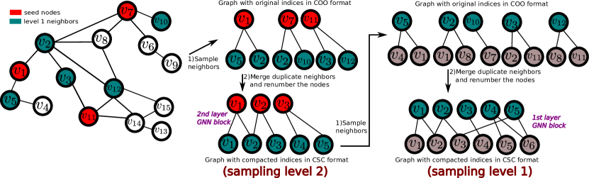
3.2. Fused sampling
The sampling operation has to be as efficient as possible as it is repeated every training iteration. Figure 1 illustrates the steps involved in sampling the graph for a 2-layer GNN in the DGL library. As described in the previous section, the sampling operation has to be executed times for an -layer GNN. Sampling level involves two steps:
-
(1)
Sampling the neighbors of the seed nodes
-
(2)
Casting the resulting graph from step 1 as a bi-partite graph, , and reordering the node indices so that they are contiguous.
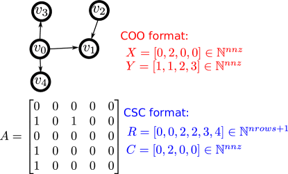
In DGL, both steps produce a graph in COO (COOrdinate) format. The preferred format for GNNs is CSC (Compressed Sparse Column) as it allows us to fetch a node’s neighbors in O(1), i.e, independently of the size of the graph. We thus need an additional step to convert from the sampled graph from the COO to the CSC format. The two formats are illustrated in Fig. 2.
The conventional 2-step approach that is applied at each sampling level involves many redundant memory movements to write the output of step 1 in COO format to memory and then read it again to compact it and convert it to CSC format. Moreover, some information that is easily accessible in step 1 has to be re-computed in step 2 such as the number of sampled neighbors of each seed nodes (which can be less than the sampling fanout if the node has few neighbors).
A CSC matrix is defined by the 2-tuple where and are the row pointer vector, and column indices vector, respectively. See Fig. 2 for the definition of and . Algorithm 1 describes our fused sampling kernel which is applied at every sampling level to yield the CSC matrix for the bi-partite graph at that level as well as the seed nodes for the next level down. Our kernel avoids the overhead of creating the intermediate COO representation. It also constructs half of the CSC representation (the vector) practically for free during the actual sampling loop, and by sampling straight into the CSC format, it avoids the expensive COO to CSC conversion. Our implementation is able to parallelize the two For loops in the algorithm and the resulting kernel accelerates sampling by a large margin compared to vanilla DGL sampling.
3.3. Distributed sampling and hybrid partitioning
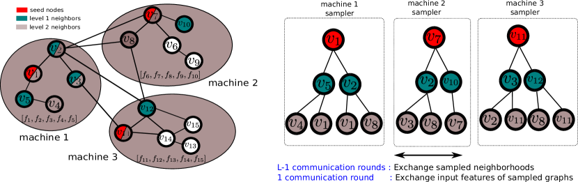
In a distributed setting, we partition the graph across multiple machines. We consider edge-cut partitioning. Each worker stores one graph partition which comprises the partition node features as well as all incoming edges to the partition nodes from all other partitions. As illustrated in Fig. 3, each machine independently samples seed nodes from the local partition, then independently samples the neighbors of these seed nodes. This can be done locally as each machine knows the neighbors of its local nodes (but not their features). All sampling levels below the top level, however, require machines to communicate. That is because each machine might need to sample the neighbors of nodes that are not in its local partition.
In general, for each sampling level after the top level, we would require two communication rounds, one round where machines submit their sampling requests to other machines, and one round where machines reply to each other with the the result of the sampling requests. For -level sampling, we thus need communication rounds to sample the graph. Since the graph features are also partitioned, two additional communication rounds are needed at the end for machines to exchange the input features of the sampled graph, bringing the total number of communication rounds to . Note that each machine creates its own local sampled graph. The GNN is trained on the local sampled graph in each machine, and the parameter gradients are then synchronized.
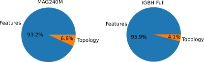
One important observation is that for many large-scale graphs, node features form the bulk of the graph size. This is illustrated in Fig. 4 for two of the largest open-source graphs currently available. Motivated by this observation, we propose to duplicate the graph topology across all machines while partitioning the relatively much larger feature tensor. Sampling the graph topology can thus proceed independently in all machines. Communication is only needed to exchange the input node features of the sampled graph, bringing the number of communication rounds from down to . We call this scheme hybrid partitioning and we show that it significantly speeds up training while keeping memory consumption per machine within reasonable limits.
4. Results
We benchmark our contributions on two popular benchmark graphs: ogbn-products and ogbn-papers100M. The graph properties are outlined in Table 1. We present results for different combinations of our techniques. We run our experiments on 2-socket machines, each equipped with two 4th Gen Intel Xeon Scalable Processors. All machines are connected by a 200Gbps Infiniband HDR fabric. In all experiments we use a 3-layer GraphSage model with hidden layer dimensions of 256. We use dropout between all layers. We use PyTorch 2.0.1 and DGL 1.1. We use FP32 numerical precision throughout. We build our FastSample library on top of DGL.
In distributed training experiments, we use torch_ccl (tor, ) as our communication backend. torch_ccl is the PyTorch wrapper for Intel’s OneCCL collective communication library (one, ). Unlike popular distributed GNN training libraries such as DistDGL (Zheng et al., 2020), we do not use point-to-point communication, but exclusively use synchronous collective communication calls such as and . We use the metis library (Karypis and Kumar, 1997) to partition the graph. Metis minimizes the number of edges that cross the partition boundaries. It balances the number of nodes and edges in each partition so that all partitions are roughly of the same size. We also assign roughly the same number of labeled nodes to each partition. Since the top level sampling seeds are drawn from the labeled nodes, equalizing the number of labeled nodes across machines ensures they all have roughly the same number of seeds and can generate the same number of graph samples during each training epoch (see Fig. 3). In distributed training experiments, we always use a batch size of 1000 per machine. We use a learning rate of 0.006.
|
|
|||||
|---|---|---|---|---|---|---|
| # nodes | 2.5M | 111M | ||||
| # edges | 124M | 3.2B | ||||
| # input features | 100 | 128 | ||||
| # classes | 47 | 172 |
4.1. Fused sampling kernel
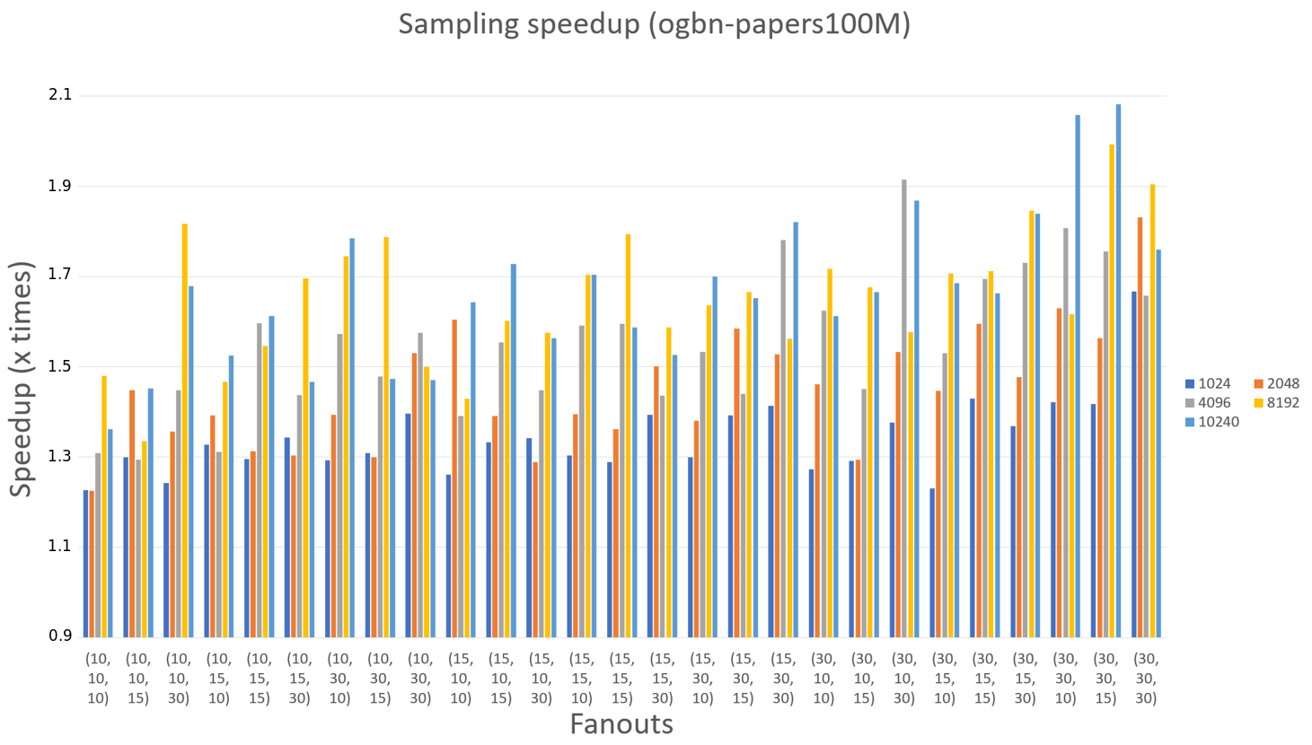
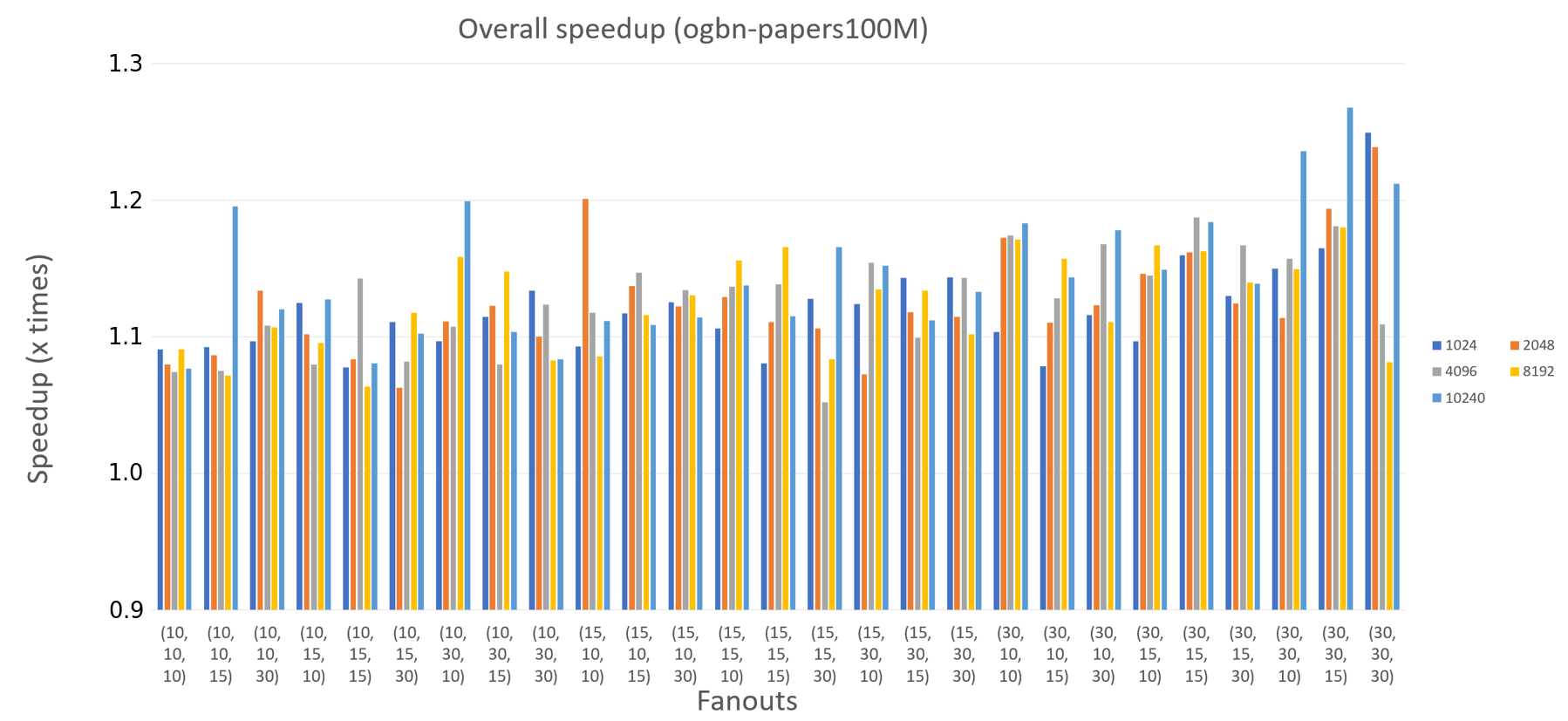
We evaluate the performance of our fused sampling kernel on ogbn-papers100M. There are two major hyper-parameters of the sampling operation: the batch size which is the number of top-level seed nodes, and the fan-out values at each sampling level. For a 3-layer GNN, the later can be written as a 3-tuple denoting the number of neighbors sampled at layers 3,2, and 1, respectively. As shown in Fig. 5, our fused sampling kernel consistently speeds up the graph sampling operation across a wide range of batch sizes and sampling fanouts. For the full training time (sampling + GNN training), we attain speedups of up to .
4.2. Hybrid partitioning
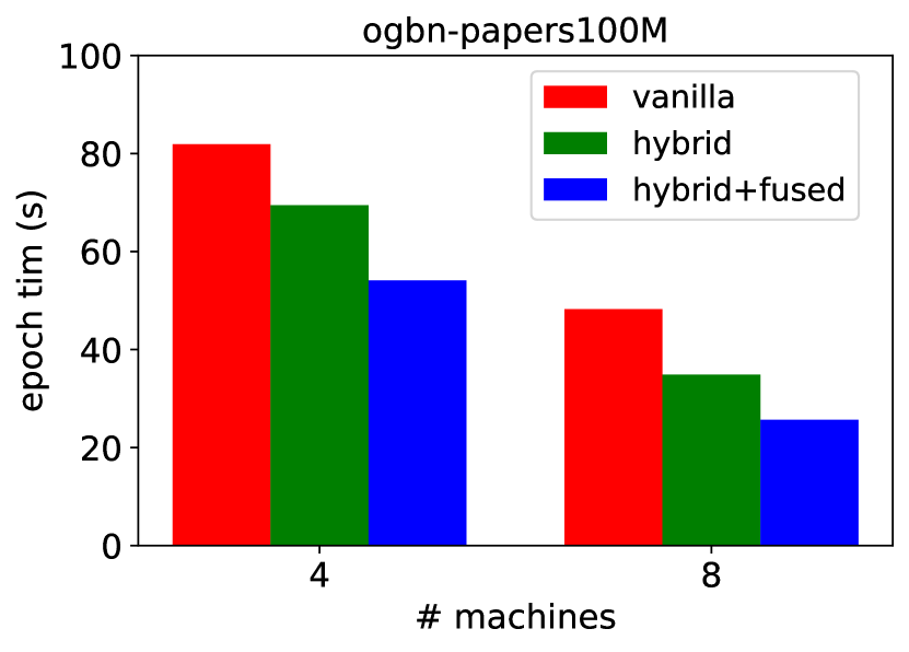
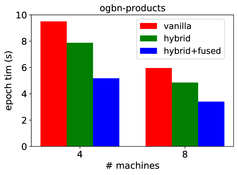
To evaluate our hybrid partitioning method, we run distributed training on 8 and 16 machines. Hybrid partitioning synergizes very well with our fused sampling kernel because the full graph topology is available on each machine and can thus be fed directly to our fused sampling kernel. Figure 6 shows the distributed training epoch times when training on ogbn-products and ogbn-papers100M. Hybrid partitioning leads to a significant reduction in epoch time. When we combine hybrid partitioning with our fused sampling kernel, we get an even bigger performance boost. Hybrid partitioning together with fused sampling reduce the per-epoch training time by almost 2X when training ogbn-papers100M on 8 machines.
Note that hybrid partitioning and fused sampling have no effect on the convergence properties of the training. Activating or disabling these two techniques lead to mathematically equivalent training results. We also note that for fair comparison, all experiments use the same training and communication software infrastructure. This ensures that any improvements on the vanilla baseline are solely due to our new methods.
5. Conclusions
Sampling-based training is becoming the method of choice to train GNNs on large graphs. As graph sizes continue to increase, distributed sampling-based training becomes the natural choice to accommodate massive graphs. In this paper, we have shown that the high-performance low-level CPU sampling kernels that are part of the DGL library, and that are in common use today, still leave plenty of performance on the table. Our fused kernel is able to consistently reduce the sampling time, in some cases accelerating the low-level graph sampling operations by up to 2X.
To make optimal use of our fused sampling kernel, we used a hybrid partitioning scheme that duplicates graph topology across all workers. The increased memory consumption per machine due to the duplicated adjacency matrix is an acceptable compromise since duplicating graph topology greatly reduces the number of communication rounds needed for sampling. The combination of hybrid partitioning and our fused sampling kernel is particularly attractive as it leaves the training iterations mathematically unchanged while greatly speeding up the distributed training (by up to 2X as shown in Fig. 6).
In the future, our work can be extended in several ways. For example, we can combine our hybrid partitioning scheme with feature caching to cache frequently accessed remote node features in order to reduce communication volume. Or we can use an adaptive fanout schedule to dynamically adjust the sampling fanouts based on the training dynamics.
References
- Ying et al. (2018) Rex Ying, Ruining He, Kaifeng Chen, Pong Eksombatchai, William L Hamilton, and Jure Leskovec. Graph convolutional neural networks for web-scale recommender systems. In Proceedings of the 24th ACM SIGKDD international conference on knowledge discovery & data mining, pages 974–983, 2018.
- Bollacker et al. (2008) Kurt Bollacker, Colin Evans, Praveen Paritosh, Tim Sturge, and Jamie Taylor. Freebase: a collaboratively created graph database for structuring human knowledge. In Proceedings of the 2008 ACM SIGMOD international conference on Management of data, pages 1247–1250, 2008.
- Tran et al. (2023) Richard Tran, Janice Lan, Muhammed Shuaibi, Brandon M Wood, Siddharth Goyal, Abhishek Das, Javier Heras-Domingo, Adeesh Kolluru, Ammar Rizvi, Nima Shoghi, et al. The open catalyst 2022 (oc22) dataset and challenges for oxide electrocatalysts. ACS Catalysis, 13(5):3066–3084, 2023.
- Bronstein et al. (2017) Michael M Bronstein, Joan Bruna, Yann LeCun, Arthur Szlam, and Pierre Vandergheynst. Geometric deep learning: going beyond euclidean data. IEEE Signal Processing Magazine, 34(4):18–42, 2017.
- Zhou et al. (2020) Jie Zhou, Ganqu Cui, Shengding Hu, Zhengyan Zhang, Cheng Yang, Zhiyuan Liu, Lifeng Wang, Changcheng Li, and Maosong Sun. Graph neural networks: A review of methods and applications. AI open, 1:57–81, 2020.
- Wu et al. (2020) Zonghan Wu, Shirui Pan, Fengwen Chen, Guodong Long, Chengqi Zhang, and S Yu Philip. A comprehensive survey on graph neural networks. IEEE transactions on neural networks and learning systems, 32(1):4–24, 2020.
- Zheng et al. (2020) Da Zheng, Chao Ma, Minjie Wang, Jinjing Zhou, Qidong Su, Xiang Song, Quan Gan, Zheng Zhang, and George Karypis. Distdgl: distributed graph neural network training for billion-scale graphs. In 2020 IEEE/ACM 10th Workshop on Irregular Applications: Architectures and Algorithms (IA3), pages 36–44. IEEE, 2020.
- Zheng et al. (2022) Da Zheng, Xiang Song, Chengru Yang, Dominique LaSalle, and George Karypis. Distributed hybrid cpu and gpu training for graph neural networks on billion-scale heterogeneous graphs. In Proceedings of the 28th ACM SIGKDD Conference on Knowledge Discovery and Data Mining, pages 4582–4591, 2022.
- Mostafa (2022) Hesham Mostafa. Sequential aggregation and rematerialization: Distributed full-batch training of graph neural networks on large graphs. Proceedings of Machine Learning and Systems, 4:265–275, 2022.
- Karypis and Kumar (1997) George Karypis and Vipin Kumar. Metis: A software package for partitioning unstructured graphs, partitioning meshes, and computing fill-reducing orderings of sparse matrices. 1997.
- Tripathy et al. (2020) Alok Tripathy, Katherine Yelick, and Aydın Buluç. Reducing communication in graph neural network training. In SC20: International Conference for High Performance Computing, Networking, Storage and Analysis, pages 1–14. IEEE, 2020.
- Md et al. (2021) Vasimuddin Md, Sanchit Misra, Guixiang Ma, Ramanarayan Mohanty, Evangelos Georganas, Alexander Heinecke, Dhiraj Kalamkar, N.K. Ahmed, and Sasikanth Avancha. Distgnn: Scalable distributed training for large-scale graph neural networks. arXiv preprin tarXiv:2104.06700, 2021.
- Wan et al. (2023) Xinchen Wan, Kaiqiang Xu, Xudong Liao, Yilun Jin, Kai Chen, and Xin Jin. Scalable and efficient full-graph gnn training for large graphs. Proceedings of the ACM on Management of Data, 1(2):1–23, 2023.
- Yang et al. (2022) Dongxu Yang, Junhong Liu, Jiaxing Qi, and Junjie Lai. Wholegraph: a fast graph neural network training framework with multi-gpu distributed shared memory architecture. In SC22: International Conference for High Performance Computing, Networking, Storage and Analysis, pages 1–14. IEEE, 2022.
- Zeng et al. (2019) Hanqing Zeng, Hongkuan Zhou, Ajitesh Srivastava, Rajgopal Kannan, and Viktor Prasanna. Graphsaint: Graph sampling based inductive learning method. arXiv preprint arXiv:1907.04931, 2019.
- Chiang et al. (2019) Wei-Lin Chiang, Xuanqing Liu, Si Si, Yang Li, Samy Bengio, and Cho-Jui Hsieh. Cluster-gcn: An efficient algorithm for training deep and large graph convolutional networks. In Proceedings of the 25th ACM SIGKDD International Conference on Knowledge Discovery & Data Mining, pages 257–266, 2019.
- Zhang et al. (2021) Bingyi Zhang, Sanmukh R Kuppannagari, Rajgopal Kannan, and Viktor Prasanna. Efficient neighbor-sampling-based gnn training on cpu-fpga heterogeneous platform. In 2021 IEEE High Performance Extreme Computing Conference (HPEC), pages 1–7. IEEE, 2021.
- Liu et al. (2021) Xin Liu, Mingyu Yan, Lei Deng, Guoqi Li, Xiaochun Ye, and Dongrui Fan. Sampling methods for efficient training of graph convolutional networks: A survey. IEEE/CAA Journal of Automatica Sinica, 9(2):205–234, 2021.
- Wang et al. (2019) Minjie Wang, Lingfan Yu, Da Zheng, Quan Gan, Yu Gai, Zihao Ye, Mufei Li, Jinjing Zhou, Qi Huang, Chao Ma, et al. Deep graph library: Towards efficient and scalable deep learning on graphs. 2019.
- Fey and Lenssen (1903) Matthias Fey and Jan Eric Lenssen. Fast graph representation learning with pytorch geometric. arxiv 2019. arXiv preprint arXiv:1903.02428, 1903.
- Tan et al. (2023) Zeyuan Tan, Xiulong Yuan, Congjie He, Man-Kit Sit, Guo Li, Xiaoze Liu, Baole Ai, Kai Zeng, Peter Pietzuch, and Luo Mai. Quiver: Supporting gpus for low-latency, high-throughput gnn serving with workload awareness. arXiv preprint arXiv:2305.10863, 2023.
- Zhu et al. (2019) Rong Zhu, Kun Zhao, Hongxia Yang, Wei Lin, Chang Zhou, Baole Ai, Yong Li, and Jingren Zhou. Aligraph: A comprehensive graph neural network platform. arXiv preprint arXiv:1902.08730, 2019.
- Min et al. (2021) Seung Won Min, Kun Wu, Sitao Huang, Mert Hidayetoğlu, Jinjun Xiong, Eiman Ebrahimi, Deming Chen, and Wen-mei Hwu. Large graph convolutional network training with gpu-oriented data communication architecture. arXiv preprint arXiv:2103.03330, 2021.
- Ma et al. (2019) Lingxiao Ma, Zhi Yang, Youshan Miao, Jilong Xue, Ming Wu, Lidong Zhou, and Yafei Dai. Neugraph: parallel deep neural network computation on large graphs. In 2019 USENIX Annual Technical Conference (USENIXATC 19), pages 443–458, 2019.
- Kaler et al. (2022) Tim Kaler, Nickolas Stathas, Anne Ouyang, Alexandros-Stavros Iliopoulos, Tao Schardl, Charles E Leiserson, and Jie Chen. Accelerating training and inference of graph neural networks with fast sampling and pipelining. Proceedings of Machine Learning and Systems, 4:172–189, 2022.
- Gandhi and Iyer (2021) Swapnil Gandhi and Anand Padmanabha Iyer. P3: Distributed deep graph learning at scale. In 15th USENIX Symposium on Operating Systems Design and Implementation (OSDI 21), pages 551–568, 2021.
- Dong et al. (2021) Jialin Dong, Da Zheng, Lin F Yang, and George Karypis. Global neighbor sampling for mixed cpu-gpu training on giant graphs. In Proceedings of the 27th ACM SIGKDD Conference on Knowledge Discovery & Data Mining, pages 289–299, 2021.
- Ramezani et al. (2020) Morteza Ramezani, Weilin Cong, Mehrdad Mahdavi, Anand Sivasubramaniam, and Mahmut Kandemir. Gcn meets gpu: Decoupling “when to sample” from “how to sample”. Advances in Neural Information Processing Systems, 33:18482–18492, 2020.
- Zou et al. (2019) Difan Zou, Ziniu Hu, Yewen Wang, Song Jiang, Yizhou Sun, and Quanquan Gu. Layer-dependent importance sampling for training deep and large graph convolutional networks. Advances in neural information processing systems, 32, 2019.
- Hu et al. (2021) Weihua Hu, Matthias Fey, Hongyu Ren, Maho Nakata, Yuxiao Dong, and Jure Leskovec. Ogb-lsc: A large-scale challenge for machine learning on graphs. arXiv preprint arXiv:2103.09430, 2021.
- Khatua et al. (2023) Arpandeep Khatua, Vikram Sharma Mailthody, Bhagyashree Taleka, Tengfei Ma, Xiang Song, and Wen-mei Hwu. Igb: Addressing the gaps in labeling, features, heterogeneity, and size of public graph datasets for deep learning research. arXiv preprint arXiv:2302.13522, 2023.
- (32) torch_ccl. https://github.com/intel/torch-ccl. Accessed: 2021-10-5.
- (33) Oneccl. https://github.com/oneapi-src/oneCCL. Accessed: 2021-10-5.