Conventional and inverse magnetocaloric and electrocaloric effects of a mixed spin-(1/2, 1) Heisenberg dimer

Abstract

The mixed spin-(1/2, 1) Heisenberg dimer accounting for two different Landé $g$-factors is exactly examined in presence of external magnetic and electric field by considering exchange as well as uniaxial single-ion anisotropies. Rigorously calculated ground-state phase diagrams affirm existence of three different types of zero-temperature phase transitions accompanied with a non-zero value of a residual entropy. Presence of a magnetoelectric effect accounted within Katsura-Nagaosa-Balatsky mechanism is demonstrated through the analyzis of the magnetization and dielectric polarization in response to both external fields. The analyzis of two basic magnetocaloric characteristics, the adiabatic change of temperature and the isothermal entropy change, achieved upon variation of external fields, are exactly calculated in order to investigate the (multi)caloric behavior. The obtained results confirm existence of both conventional as well as inverse magnetocaloric effects. Utilizing the refrigeration capacity coefficient it is found that the application of an electric field during the adiabatic demagnetization process may lead to an enhancement of cooling performance in the region of conventional magnetocaloric effect. On the other hand, a sufficiently large electric field can reduce an inverse caloric effect provided that the electric-field-induced transition from the fully to partially polarized state is realized.

1 Introduction

Low-dimensional quantum spin models traditionally belong to the most intensively studied magnetic systems. A low-dimensionality promoting extraordinary strong quantum fluctuations is at an origin of considerable diversity of unconventional properties such as a quantum entanglement Wootters ; Souza ; Horodecki ; Rojas2012 ; Cenci20 ; Cenci21 ; Varga21 , existence of plateaus or quasi-plateaus in magnetization curves Honecker ; Ohanyan2015 ; Cenci18 , quantum spin-liquid state Lacroix ; Imambekov or magnetoelectric Sharples ; Baran ; Cenci98 ; Ohanyan20 effect, which makes low-dimensional quantum spin systems very promising for various technological applications in modern smart devices. Beside to this, an enormous proliferation in an investigation of low-dimensional quantum materials may be connected to their utilization in quantum communication and quantum information processing Markham ; Matthews ; Rahaman .

Caloric effects, which are characterized as temperature changes of a physical system upon variation of applied external magnetic and/or electric field, are further extraordinary features of low-dimensional quantum spin systems referred to as magnetocaloric and electrocaloric phenomenon Fu ; Oliveira ; Torrico ; Szalowski2019 ; Mischenko ; Moya14 ; Szalowski18 . An effort aimed at deeper understanding of both unconventional caloric processes has stimulated vigorous researcher’s activities, bearing in mind the fact that the solid-state cooling/heating technologies are environmentally more friendly alternative with respect to a conventional vapor-cycle refrigeration Glanz . In addition, the wide utilization of aforementioned phenomena in the ultra-low cryogenics, room temperature cooling or cooling of (micro)electronic components, makes materials with a substantial caloric response very demanding for various spheres of a life. Despite the energetically and thus economically higher convenience of an electrocaloric effect (ECE), the magnetocaloric effect (MCE) was to date a more thoroughly investigated Ismail . A few recent studies devoted to the concept of multicaloric materials argued that the MCE could be maximized by an external electric field Ursic ; Qiao ; Szalowski21 . Due to a complexity of processes responsible for existence of such intricate behavior there exists only a few theoretical studies dealing with the multicaloric behavior of low-dimensional quantum spin systems Baran ; Szalowski18 ; Zad ; Ding ; Richter ; Fodouop . For this reason, we would like to contribute to this novel research area with a goal to extend knowledge about the maximization of caloric processes in solid-state magnetic insulators.

It should be emphasized that various caloric processes can be in general accompanied by relieving or consuming of an additional heat, which is macroscopically detectable as a heating or a cooling of a system environment. The conventional caloric effect refers to the positive isothermal entropy change and negative adiabatic temperature change achieved upon the variation of an external field, while the negative isothermal entropy change and positive adiabatic temperature change is termed as an inverse caloric effect. The inverse MCE was for instance reported for different kinds of antiferromagnetic, ferrimagnetic or paramagnetic compounds Ranke ; Krenke1 ; Krenke2 ; Sandeman ; Nayak ; Biswas , while the inverse ECE has been observed in ferroelectric Udin ; Geng and antiferroelectric materials specifically restricted to a certain temperature and field regions Perantie ; LeGoupil . A coexistence of both conventional and inverse caloric phenomena is rarely also possible for advanced multifunctional materials with an extraordinary magnetic phase diagram Szalowski21 ; Derzhko ; Pereira ; Verkholyak ; Szalowski ; Galisova ; Krishnamoorthi ; Diop ; Odaira ; Burzo ; Zhang2010 ; Reis . In connection to this, the partial aim of this study is to examine the possibility to generate different types of thermal changes (the cooling or heating) utilizing peculiar properties of heterogeneous low-dimensional quantum spin systems.

From the theoretical point of view, the quantum Heisenberg model and its diverse variants represent a good theoretical tool to study low-dimensional quantum spin systems, which allow due to their relative simplicity a rigorous examination of quantum phenomena in their purest nature Gatteschi ; Kahn ; Hieida ; Dmitriev04 ; Hikihara ; Hagemans ; Caux ; Menchyshyn ; Brockmann ; Chen ; Bacq ; Cu ; Ivanov ; Rojas2017 ; Rojas2019 ; Strecka20 . Especially, the following works focusing on the study of thermodynamic and magnetic properties of various Heisenberg dimers Furrer ; Haraldsen ; Efremov ; Whangbo are rewarding to better understand peculiar properties of single molecular magnets. In the present paper we will focus our attention on one of the simplest Heisenberg models, namely, a mixed spin-(1/2, 1) Heisenberg dimer, which involves two different types of magnetic ions. The choice of the magnetically asymmetric system has been performed for two reasons. The first one originates from the fact, that the mixed spin-(1/2, 1) Heisenberg dimer very well approximates a distinct group of bimetallic low-dimensional molecular magnets like that reported in Refs. Kahn ; Gleizes ; Hagiwara2 ; Koningsbruggen ; Hagiwara ; Pei . And the second one originates from the knowledge, that the imbalance between magnetic ions leads to the modification of excitation spectra Houchins , which can be a conceptus of different caloric properties. The application of the additional electric field on such simple quantum system in connection to the possible enhancement of MCE is a supplemental task of our theoretical analyzis.

The paper is organized as follows. In Sec. 2 we briefly introduce the model under the investigation along with relevant quantities required for a study of ground-state and thermodynamic properties. The most interesting results demonstrating the influence of both magnetic as well as electric field on the ground-state spin arrangement, total magnetization, dielectric polarization and entropy are discussed in Sec. 3. The dominant part of Sec. 3 is focused on the study of magnetocaloric properties and their modulation caused by the varied electric field. A summary of the most important findings are presented in Sec. 4.

2 Model and Method

Let us consider a mixed spin-(1/2, 1) Heisenberg dimer defined through the Hamiltonian

$$\hat{\cal H} =J\left[\Delta(\hat{S}^{x}_{1}\hat{\mu}^{x}_{2}\!+\!\hat{S}^{y}_{1}\hat{\mu}^{y}_{2})\!+\!\hat{S}^{z}_{1}\hat{\mu}^{z}_{2}\right]\!+\!D(\hat{\mu}^{z}_{2})^{2}\!-\!\mu_{B}B(g_{1}\hat{S}^{z}_{1}\!+\!g_{2}\hat{\mu}^{z}_{2})\!+\!E(\hat{S}^{x}_{1}\hat{\mu}^{y}_{2}\!-\!\hat{S}^{y}_{1}\hat{\mu}^{x}_{2}).$$ (1)

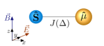
Figure 1: A schematic representation of a mixed spin-(1/2, 1) Heisenberg dimer defined through the Hamiltonian (1) and situated along $x$-axis. Blue (small) ball illustrates the spin-1/2 magnetic ion and yellow (large) ball illustrates the spin-1 magnetic ion coupled through the exchange constant $J(\Delta)$. External magnetic field ($\widearrow{B}$) is applied along the $z$-axis, while the external electric field ($\widearrow{E}$) is applied along the $y$-axis.

The symbols $\hat{S}^{\alpha}_{1}$ and $\hat{\mu}^{\alpha}_{2}$ ($\alpha\!=\!x,y,z$) denote spatial components of spin-1/2 and 1 operators, the parameter $J$ characterizes the exchange interaction with the XXZ exchange anisotropy parameter $\Delta$ and the parameter $D$ corresponds to the uniaxial single-ion anisotropy acting exclusively on the spin-1 magnetic ion. The external magnetic field $\widearrow{B}\!=\!(0,0,B)$ applied along $z$-axis is responsible for existence of the standard Zeeman’s term in the Hamiltonian (1), while the external electric field applied along $y$-direction $\widearrow{E}\!=\!(0,E_{y},0)$ is being responsible for other non-zero contribution denoted by the electric field energy $E$. Both external fields are perpendicular to a link connecting both spin species lying along $x$-axis (see Fig. 1). Finally, $g_{1}$ and $g_{2}$ are Landé $g$-factors of the spin-1/2 and spin-1 magnetic ions, respectively, the symbol $\mu_{B}$ stands for Bohr magneton. The specific form of the electric field energy follows from the inverse Dzyaloshinskii-Moriya mechanism referred to as Katsura-Nagaosa-Balatsky (KNB) mechanism Katsura ; Jia , according to which the dielectric polarization of the pair of interacting spins $\hat{\mathbf{S}}_{1}$ and $\hat{\bm{\mu}}_{2}$ is connected to the following expression

$$\hat{\mathbf{P}}_{12}\!\varpropto\!{\widearrow{\rm e}}_{12}\!\times\!\hat{\mathbf{S}}_{1}\!\times\!\hat{\bm{\mu}}_{2},$$ (2)

where ${\widearrow{\rm e}}_{12}$ is the unit vector pointing from site 1 to site 2. In the present case the magnetic ions are positioned along the $x$-axis, i.e. $\widearrow{\rm e}_{12}\!=\!(1,0,0)$, and hence, the spatial components of the dielectric polarization according to the KNB mechanism are quite simple

$$\hat{P}_{x}\!=\!0,\hskip 28.45274pt\hat{P}_{y}\!\varpropto\!\hat{S}^{y}_{1}\hat{\mu}^{x}_{2}\!-\!\hat{S}^{x}_{1}\hat{\mu}^{y}_{2},\hskip 28.45274pt\hat{P}_{z}\!\varpropto\!\hat{S}^{z}_{1}\hat{\mu}^{x}_{2}\!-\!\hat{S}^{x}_{1}\hat{\mu}^{z}_{2}.$$ (3)

It directly follows from Eq. (3) that a specific spatial orientation of the external electric field applied along the $y$-axis leads to the particular form of the Hamiltonian (1), which exemplifies the energy contribution $E$ of the external electric field on the mixed spin-(1/2, 1) Heisenberg dimer by means of the effective Dzyaloshinskii-Moriya term $E(\hat{S}^{x}_{1}\hat{\mu}^{y}_{2}\!-\!\hat{S}^{y}_{1}\hat{\mu}^{x}_{2})$. In addition, the effective Dzyaloshinskii-Moriya term determines, up to the unimportant constant $\mu$, also the dielectric polarization $P\!\equiv\!\langle\hat{P}_{y}\rangle\!=\!\mu\langle\hat{S}^{y}_{1}\hat{\mu}^{x}_{2}\!-\!\hat{S}^{x}_{1}\hat{\mu}^{y}_{2}\rangle$, whereby the microscopic constant $\mu$ depends on quantum chemical features of the bond connecting two magnetic ions Katsura ; Jia .

The matrix representation of the Hamiltonian (1) constructed in a standard basis of eigenstates of $z$-components of both spin operators $|\varphi_{i}\rangle\!\equiv\!|S^{z}_{1},\mu^{z}_{2}\rangle\!\in\!\{|\frac{1}{2},1\rangle,|\frac{1}{2},0\rangle,|\frac{1}{2},-1\rangle,|\!-\!\frac{1}{2},1\rangle,|\!-\!\frac{1}{2},0\rangle,|\!-\!\frac{1}{2},-1\rangle\}$ takes a relative simple (sparse) form

$$\left\langle\varphi_{j}\right|\hat{\cal H}\left|\varphi_{i}\right\rangle=\left(\begin{array}[]{cccccc}{\cal H}_{11}&0&0&0&0&0\\ 0&{\cal H}_{22}&0&{\cal H}_{24}&0&0\\ 0&0&{\cal H}_{33}&0&{\cal H}_{35}&0\\ 0&{\cal H}_{42}&0&{\cal H}_{44}&0&0\\ 0&0&{\cal H}_{53}&0&{\cal H}_{55}&0\\ 0&0&0&0&0&{\cal H}_{66}\end{array}\right)$$ (10)

with the following six diagonal elements ${\cal H}_{ii}$ ($i\!=\!1,2,\dots,6$)

$${\cal H}_{11}\! =\!\frac{1}{2}\left[J\!+\!2D\!-\!(h_{1}\!+\!2h_{2})\right],\hskip 28.45274pt{\cal H}_{22}\!=\!-{\cal H}_{55}\!=\!-\frac{h_{1}}{2},\hskip 28.45274pt{\cal H}_{33}\!=\!-\frac{1}{2}\left[J\!-\!2D\!+\!(h_{1}\!-\!2h_{2})\right],$$

$${\cal H}_{44}\! =\!-\frac{1}{2}\left[J\!-\!2D\!-\!(h_{1}\!-\!2h_{2})\right],\hskip 21.33955pt{\cal H}_{66}\!=\!\frac{1}{2}\left[J\!+\!2D\!+\!(h_{1}\!+\!2h_{2})\right].$$ (11)

In above expressions two new parameters $h_{1,2}\!=\!g_{1,2}\mu_{B}B$ have been introduced with the aim to simplify the mathematical notation of further relevant quantities. Four remaining non-zero off-diagonal elements are complex due to the last term of Eq. (1), which has character of antisymmetric Dzyaloshinskii-Moriya interaction originating from the external electric field applied along the $y$-axis. Thus, the non-zero off-diagonal terms can be unambiguously characterized by the argument $\varphi\!=\!\arctan\left(\frac{E}{J\Delta}\right)$ through the following formulas

$${\cal H}_{24}\! =\!{\cal H}_{35}\!=\!\frac{{\rm e}^{i\varphi}}{\sqrt{2}}\sqrt{(J\Delta)^{2}\!+\!E^{2}},\hskip 28.45274pt{\cal H}_{42}\!=\!{\cal H}_{53}\!=\!\frac{{\rm e}^{-i\varphi}}{\sqrt{2}}\sqrt{(J\Delta)^{2}\!+\!E^{2}}.$$ (12)

After a straightforward diagonalization of the Hamiltonian (10) one can obtain a complete energy spectrum involving six different eigenvalues and respective eigenvectors

$$\varepsilon_{1,2}= \frac{1}{2}\left[J\!+\!2D\!\mp\!(h_{1}\!+\!2h_{2})\right],\hskip 184.9429pt|\psi_{1,2}\rangle=|\!\pm\!\tfrac{1}{2},\pm 1\rangle,$$ (13)

$$\varepsilon_{3,4}= -\frac{1}{4}\left(J\!-\!2D\!+\!2h_{2}\right)\!\mp\!\frac{1}{4}\sqrt{\left[J\!-\!2D\!-\!2(h_{1}\!-\!h_{2})\right]^{2}\!+\!8\left[(J\Delta)^{2}\!+\!E^{2}\right]},\hskip 14.22636pt|\psi_{3,4}\rangle={\rm e}^{i\varphi}|c_{1}^{\mp}||\tfrac{1}{2},0\rangle\!\mp\!|c_{1}^{\pm}||\!-\!\tfrac{1}{2},1\rangle,$$ (14)

$$\varepsilon_{5,6}= -\frac{1}{4}\left(J\!-\!2D\!-\!2h_{2}\right)\!\mp\!\frac{1}{4}\sqrt{\left[J\!-\!2D\!+\!2(h_{1}\!-\!h_{2})\right]^{2}\!+\!8\left[(J\Delta)^{2}\!+\!E^{2}\right]},\hskip 14.22636pt|\psi_{5,6}\rangle={\rm e}^{i\varphi}|c_{2}^{\pm}||\tfrac{1}{2},-1\rangle\!\mp\!|c_{2}^{\mp}||\!-\!\tfrac{1}{2},0\rangle.$$ (15)

The modulus of complex coefficients of four nonseparable quantum entangled states $|\psi_{3,4}\rangle$ and $|\psi_{5,6}\rangle$ are explicitly defined by the following relations

$$|c_{1}^{\pm}| =\frac{1}{\sqrt{2}}\sqrt{1\!\pm\!\frac{J\!-\!2D\!-\!2(h_{1}\!-\!h_{2})}{\sqrt{\left[J\!-\!2D\!-\!2(h_{1}\!-\!h_{2})\right]^{2}\!+\!8\left[(J\Delta)^{2}\!+\!E^{2}\right]}}},\hskip 14.22636pt|c_{2}^{\pm}|=\frac{1}{\sqrt{2}}\sqrt{1\!\pm\!\frac{J\!-\!2D\!+\!2(h_{1}\!-\!h_{2})}{\sqrt{\left[J\!-\!2D\!+\!2(h_{1}\!-\!h_{2})\right]^{2}\!+\!8\left[(J\Delta)^{2}\!+\!E^{2}\right]}}}.$$ (16)

With the help of a complete set of energy eigenvalues (13)-(15) one may obtain an exact analytical expression for the partition function ${\cal Z}$

$${\cal Z}\!=\!\sum_{i=1}^{6}{\rm e}^{-\varepsilon_{i}/k_{B}T}$$ (17)

where $k_{B}$ is a Boltzmann’s constant and $T$ is the absolute temperature. The exact analytic expression for the partition function is for brevity explicitly given in Appendix, Eq. (32). Having an explicit expression for the partition function (17) one can easily derive the free energy $F\!=\!-k_{B}T\ln{\cal Z}$ and subsequently all thermodynamic functions relevant for the analyzis of magnetoelectric properties. In particular, the total magnetization $m$ normalized with respect to the saturation magnetization $m_{s}$

$$\frac{m}{m_{s}} \!=\!-\frac{\partial F}{\partial\mu_{B}B}$$ (18)

and the dielectric polarization $P$ follows from the formula

$$P\! =\!-\mu\frac{\partial F}{\partial E},$$ (19)

which will be from here onward considered in dimensionless units by setting the microscopic constant $\mu\!=\!1$. Analyzing the explicit form of both formulas, explicitly listed in Appendix as Eq. (33) and Eq. (34), one immediately deduces that the magnetization and dielectric polarization become zero in absence of external magnetic and electric fields, respectively, what immediately precludes existence of a spontaneous multiferroic behavior. From the point of view of ECE and MCE properties the most essential quantity is the magnetic entropy $S$, defined as

$$\displaystyle S =-\frac{\partial F}{\partial T},$$ (20)

whose exact analytic formula is for completeness given in Appendix, Eq. (35).

3 Results and discussion

In this section, we will proceed to a discussion of the most interesting results obtained for the mixed spin-(1/2, 1) Heisenberg dimer in a presence of the external magnetic and electric fields with the particular emphasis laid on conventional and inverse caloric effects. Our analyzis will be restricted to the particular case with the antiferromagnetic fully isotropic exchange coupling $J\!>\!0$, $\Delta\!=\!1$, which however reflects all generic features of the investigated quantum spin model even for a more general case with $\Delta\!\neq\!1$ as well. For simplicity, the Landé $g$-factor of the spin-1/2 magnetic ion is fixed to the value $g_{1}\!=\!2$, whereas the Landé $g$-factor of the spin-1 magnetic ion $g_{2}$ will be varied.

3.1 Ground state

It turns out that the mixed spin-(1/2, 1) Heisenberg dimer has in total three different ground states, which can be characterized via the following eigenvectors and eigenenergies

$$|{\rm F}_{\pm}\rangle =|\!\pm\!\tfrac{1}{2},\pm 1\rangle,\hskip 99.58464pt\varepsilon_{\rm F_{\pm}}=\frac{1}{2}\left[J\!+\!2D\!\mp\!(h_{1}\!+\!2h_{2})\right],$$

$$|{\rm QF_{+}}\rangle ={\rm e}^{i\varphi}|c_{1}^{-}||\tfrac{1}{2},0\rangle\!-\!|c_{1}^{+}||\!-\!\tfrac{1}{2},1\rangle,\hskip 17.07182pt\varepsilon_{\rm QF_{+}}=-\frac{1}{4}\left(J\!-\!2D\!+\!2h_{2}\right)\!-\!\frac{1}{4}\sqrt{\left[J\!-\!2D\!-\!2(h_{1}\!-\!h_{2})\right]^{2}\!+\!8\left[(J\Delta)^{2}\!+\!E^{2}\right]},$$

$$|{\rm QF_{-}}\rangle =|c_{2}^{-}||\!-\!\tfrac{1}{2},0\rangle\!-\!{\rm e}^{i\varphi}|c_{2}^{+}||\tfrac{1}{2},-1\rangle,\hskip 8.5359pt\varepsilon_{\rm QF_{-}}=-\frac{1}{4}\left(J\!-\!2D\!-\!2h_{2}\right)\!-\!\frac{1}{4}\sqrt{\left[J\!-\!2D\!+\!2(h_{1}\!-\!h_{2})\right]^{2}\!+\!8\left[(J\Delta)^{2}\!+\!E^{2}\right]}.$$

Evidently, the fully polarized ferromagnetic ground state $|{\rm F}_{\pm}\rangle$ is two-fold degenerate in absence of an external magnetic field, but an arbitrary small but non-zero magnetic field lift this two-fold degeneracy as both spins are fully polarized to the magnetic-field direction. The quantum ferrimagnetic ground states $|{\rm QF}_{\pm}\rangle$ differing from each other by the sign of a $z$-component of the total spin (the ’$+$’ sign for the $|{\rm QF}_{+}\rangle$ phase and the ’$-$’ sign for the $|{\rm QF}_{-}\rangle$ phase) are also energetically equivalent in the zero magnetic field. It should be emphasized that the obtained results are in a good correspondence with previous observations Cenci20 , because the quantum ferrimagnetic ground state $|{\rm QF}_{-}\rangle$ emerges in the ground-state phase diagram just in the case of low enough $g_{2}/g_{1}$ ratio obeying the condition

$$\frac{g_{2}}{g_{1}}\! \leq\!\left\{1+\sqrt{1\!+\!8\frac{(J\Delta)^{2}\!+\!E^{2}}{(J\!-\!2D)^{2}}}\right\}^{-1}\!\lesssim\!\frac{1}{2},$$ (21)

which ensures a positive total magnetization in spite of the negative total spin. In addition, the existence of the quantum ferrimagnetic phase $|{\rm QF}_{-}\rangle$ with the negative sign of the total spin is strongly determined by the specific value of an uniaxial single-ion anisotropy $D/J$ given at least by one of the following conditions

$$\varepsilon_{\rm QF_{-}}\!\leq\!\varepsilon_{\rm F_{+}}:D\!\leq\!\frac{1}{2}\left[2\left(h_{1}\!+\!h_{2}\right)\!-\!J\!-\!\frac{(J\Delta)^{2}\!+\!E^{2}}{(2h_{2}\!-\!J)}\right],\hskip 28.45274pt\varepsilon_{\rm QF_{-}}\!\leq\!\varepsilon_{\rm QF_{+}}:|J\!-\!2D|\!\geq\!2h_{2}\sqrt{1\!+\!\frac{2[(J\Delta)^{2}\!+\!E^{2}]}{h_{1}(h_{1}\!-\!2h_{2})}}.$$ (22)

Fig. 2 illustrates the typical ground-state phase diagrams in the $E/J-\mu_{B}B/J$ plane for the ratio $g_{2}/g_{1}$ above (Fig. 2$(a)$) and below (Fig. 2$(b)$) the critical ratio of the Landé $g$-factors, $g_{2}/g_{1}\!\approx\!1/2$.

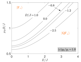
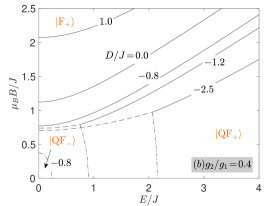
Figure 2: Ground-state phase diagrams in the $E/J\!-\!\mu_{B}B/J$ plane for a few selected values of the uniaxial single-ion anisotropy $D/J$, $\Delta\!=\!1.0$ and the two different ratios of the $g$-factors: $(a)$ $g_{2}/g_{1}\!=\!1$ and $(b)$ $g_{2}/g_{1}\!=\!0.4$. The displayed lines in all panels correspond to the phase boundaries: $|{\rm QF}_{+}\rangle$-$|{\rm F}_{+}\rangle$ (solid lines), $|{\rm QF}_{-}\rangle$-$|{\rm F}_{+}\rangle$ (dashed lines) and $|{\rm QF}_{-}\rangle$-$|{\rm QF}_{+}\rangle$ (dashed-dotted lines), respectively.

The ground-state phase diagram has for each $g_{2}/g_{1}\!>\!1/2$ a very simple structure with just two phases, $|{\rm QF}_{+}\rangle$ and $|{\rm F}_{+}\rangle$, which have the equivalent energies at the magnetic fields restricted by the condition

$$|{\rm QF}_{+}\rangle-|{\rm F}_{+}\rangle:\mu_{B}B\!=\!\frac{1}{4}\left[\left(\frac{J\!+\!2D}{g_{2}}\!+\!\frac{2J}{g_{1}}\right)\!+\!\sqrt{\left(\frac{J\!+\!2D}{g_{2}}\!-\!\frac{2J}{g_{1}}\right)^{2}\!+\!\frac{8\left[(J\Delta)^{2}\!+\!E^{2}\right]}{g_{1}g_{2}}}\right].$$ (23)

It is obvious from Eq. (23) that the increasing $g_{2}/g_{1}$ ratio and/or decreasing value of the uniaxial single-ion anisotropy $D/J$ support the effect of the magnetic field to reorient magnetic moments of both ions into its direction. The typical structure of the ground-state phase diagram for $g_{2}/g_{1}<1/2$ is presented in Fig. 2$(b)$. Above the threshold magnetic field $\mu_{B}B_{t}/J$ the ground-state phase diagram is quite reminiscent of the one discussed above, whereas below this threshold magnetic field both quantum ferrimagnetic phases $|{\rm QF}_{\pm}\rangle$ coexist together whenever the condition is met

$$|{\rm QF}_{-}\rangle-|{\rm QF}_{+}\rangle:\mu_{B}B\!=\!\frac{1}{2}\sqrt{\left(\frac{J\!-\!2D}{g_{2}}\right)^{2}\!-\!\frac{8[\left(J\Delta\right)^{2}\!+\!E^{2}]}{g_{1}(g_{1}-2g_{2})}}.$$ (24)

Obviously, the decreasing uniaxial single-ion anisotropy enlarges the stability region of the peculiar quantum ferrimagnetic phase with the negative total spin $|{\rm QF}_{-}\rangle$ separated from the fully polarized $|{\rm QF}_{+}\rangle$ phase by the condition

$$|{\rm QF}_{-}\rangle-|{\rm F}_{+}\rangle:\mu_{B}B\!=\!\frac{1}{4}\left[\left(\frac{J\!+\!2D}{(g_{1}\!+\!g_{2})}\!+\!\frac{J}{g_{2}}\right)\right.\!+\!\left.\sqrt{\left(\frac{J\!+\!2D}{(g_{1}\!+\!g_{2})}\!-\!\frac{J}{g_{2}}\right)^{2}\!+\!\frac{4\left[\left(J\Delta\right)^{2}\!+\!E^{2}\right]}{g_{2}(g_{1}\!+\!g_{2})}}\right].$$ (25)

3.2 Magnetoelectric effect

Now, let us look at the magnetoelectric effect of the mixed spin-(1/2, 1) Heisenberg dimer. In the most general characteristic, the magnetoelectric effect could be determined through the magnetic-field dependence of the dielectric polarization and vice versa the electric-field dependence of the magnetization. The relative size of dielectric polarization (34) is a direct consequence of the applied electric and magnetic fields, whereas the magnetic field by itself cannot induce the dielectric polarization in absence of the external electric field. Consequently, the spontaneous ferroelectricity of the mixed spin-(1/2, 1) Heisenberg dimer is prohibited. On the other hand, the ground-state magnetization normalized with respect to its saturation value $m/m_{s}$ in the quantum ferrimagnetic phases $|{\rm QF}_{\pm}\rangle$ is a monotonically decreasing function of the electric field energy $E$ even in absence of the external magnetic field

$$\lim_{\frac{\mu_{B}B}{J}\to 0}\langle{\rm QF}_{\pm}|\frac{m}{m_{s}}|{\rm QF}_{\pm}\rangle\!=\!\frac{1}{g_{1}\!+\!2g_{2}}\left[\pm g_{2}\!\mp\!\frac{(g_{1}\!-\!g_{2})\left(J\!-\!2D\right)}{\sqrt{\left[(J\!-\!2D\right)^{2}\!+\!8\left[(J\Delta)^{2}\!+\!E^{2}\right]}}\right].$$ (26)

Note furthermore that arbitrarily small but non-zero thermal fluctuations completely destroy the spontaneous magnetization. The behavior of the magnetization and dielectric polarization are demonstrated in Figs. 3-4 for a few selected sets of model parameters in presence of both external fields.

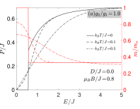
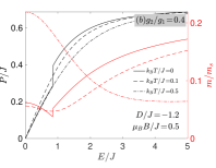
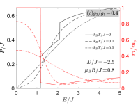
Figure 3: The dielectric polarization $P/J$ (left $y$-axis) and normalized magnetization $m/m_{s}$ (right $y$-axis) as a function of the dimensionless electric field energy $E/J$ calculated for three temperatures and selected set of model parameters indicated in panels.

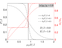
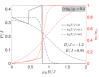
Figure 4: The dielectric polarization $P/J$ (left $y$-axis) and normalized magnetization $m/m_{s}$ (right $y$-axis) as a function of the magnetic field $\mu_{B}B/J$ calculated for three temperatures and selected set of model parameters indicated in panels.

At zero temperature both quantities exhibit stepwise changes in a vicinity of all field-driven phase transitions, which gradually smear out upon increasing of temperature. The zero-temperature dependence of the dielectric polarization on the electric field energy (Fig. 3) demonstrate three different regimes conditioned by the ground-state spin arrangement. The zero-temperature value of dielectric polarization corresponding to the classical ferromagnetic phase $|{\rm F}_{+}\rangle$ is a constant function with respect to the electric field energy with a zero magnitude, i.e. $P_{\rm F_{+}}/J\!=\!0$, whereas the dielectric polarization corresponding to the quantum ferrimagnetic phases $|{\rm QF}_{\mp}\rangle$ depends on the electric field and magnetic field thorough the following relations

$$P_{\rm QF_{\pm}}\!=\!\frac{2E}{\sqrt{\left[J\!-\!2D\!\mp\!2(h_{1}\!-\!h_{2})\right]^{2}\!+\!8[\left(J\Delta\right)^{2}\!+\!E^{2}]}}.$$ (27)

In agreement with general expectations, the increasing electric field enhances the dielectric polarization, while the increasing magnetic field can reduce or enhance the dielectric polarization at low enough temperatures as a result of different dielectric responses of the quantum ferrimagnetic ground states $|{\rm QF}_{+}\rangle$ and $|{\rm QF}_{-}\rangle$, respectively (Figs. 4$(b)$ and $(c)$). It has been found, furthermore, that such extraordinary behavior can be detected if and only if $g_{2}/g_{1}\!\neq\!1$, because the identical values of Landé $g$-factors make the dielectric polarization (27) fully independent of the magnetic field.

Analyzing in detail the behavior of magnetization, one may reach the following interesting observations. (i) The ground-state magnetizations of the quantum ferrimagnetic phases $|{\rm QF}_{\pm}\rangle$ are in general complex non-linear functions of the magnetic field

$$\langle{\rm QF}_{\pm}|\frac{m}{m_{s}}|{\rm QF}_{\pm}\rangle\!=\!\frac{1}{g_{1}\!+\!2g_{2}}\left[\pm g_{2}\!\mp\!\frac{(g_{1}\!-\!g_{2})\left[J\!-\!2D\!\mp\!2(h_{1}\!-\!h_{2})\right]}{\sqrt{\left[(J\!-\!2D\!\mp\!2(h_{1}\!-\!h_{2})\right]^{2}\!+\!8\left[(J\Delta)^{2}\!+\!E^{2}\right]}}\right].$$ (28)

(ii) The zero-temperature magnetization exhibits a significant local minimum as a function of the electric field energy at its specific value, which appears in the vicinity of the electric-field driven phase transition between both quantum ferrimagnetic ground states $|{\rm QF}_{\pm}\rangle$ [Fig. 3$(b)$ and $(c)$]. (iii) The magnetization of the quantum ferrimagnetic $|{\rm QF}_{+}\rangle$ phase saturating at $m/m_{s}\!=\!1/3$ for the fully isotropic case $g_{2}/g_{1}\!=\!1$ changes its curvature as well as its position when considering the anisotropic case $g_{2}/g_{1}\!\neq\!1$ [see Figs. 4$(b)$ and $(c)$]. Owing to this fact, the magnetization quasi-plateau can be observed at moderate magnetic fields instead of the true one-third magnetization plateau. The magnetization quasi-plateau connected to the $|{\rm QF}_{+}\rangle$ phase is positioned below the value $m/m_{s}\!=\!1/3$ for $g_{2}/g_{1}\!<\!1$, whereas the magnetization quasi-plateau for $g_{2}/g_{1}\!>\!1$ is always detected above the value $m/m_{s}\!>\!1/3$. Besides, the non-zero electric field stabilizes existence of quasi-plateaus in response to the magnetic field and/or temperature, because the increasing electric field energy has tendency to align magnetic moments in a perpendicular direction with respect to the applied magnetic field. The ground-state magnetization corresponding to the other quantum ferrimagnetic $|{\rm QF}_{-}\rangle$ phase again leads to the quasi-plateau, which converges to $m/m_{s}\!=\!0$ as one approaches the zero magnetic field. It can be deduced from Figs. 3 and 4 that the striking magnetization quasi-plateau is perfectly mirrored also in a quasi-plateau behavior of the dielectric polarization, which markedly demonstrates the magnetoelectric coupling in zero as well as non-zero temperatures of the mixed spin-(1/2, 1) Heisenberg dimer.

3.3 Magnetocaloric and electrocaloric properties

In order to study the magnetocaloric and electrocaloric properties of a mixed spin-(1/2, 1) Heisenberg dimer we will analyze in detail the adiabatic changes of temperature achieved upon variation of the external magnetic or electric field. It should be expected that in the proximity of a certain field-driven phase transition, the competition between all driving forces can lead to the more or less rapid change of temperature, however the system entropy remains fixed. The slope as well as the distance of two neighboring temperatures are two crucial identifiers of intensity of cooling process. The density plots of the entropy as a function of temperature and magnetic field are presented in Fig. 5. For isentropic changes of temperature driven exclusively by an applied magnetic field ($E/J\!=\!0.0$) we identify three different scenarios.

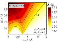
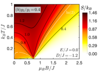
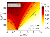
Figure 5: Density plots of the entropy in the magnetic field versus temperature plane for three selected sets of the model parameters in absence of an applied electric field. Displayed curves in all panels demonstrate isentropic lines, among which particular isentropy lines with $S/k_{B}\!=\!\ln(2)$ are highlighted by a white color.

The density plot of the entropy for high enough ratio $g_{2}/g_{1}$ between Landé $g$-factors, for which only the $|{\rm F}_{+}\rangle$ and $|{\rm QF}_{+}\rangle$ ground states are available, is presented in Fig. 5$(a)$. It is quite apparent that the most prominent adiabatic change of temperature is observed close to the value of the residual entropy $S/k_{B}\!=\!\ln(2)$, along which the temperature drops infinitely fast in the vicinity of the transition field between $|{\rm QF}_{+}\rangle$-$|{\rm F}_{+}\rangle$ phases. Almost identical temperature change is identified very close to zero magnetic field, where two-fold degeneracy is lifted by an arbitrarily small non-zero magnetic field. Because the single-ion anisotropy $D/J$ reduces the effect of magnetic field, its increasing magnitude can be used as an additional tuning parameter for enlargement of the temperature interval with an infinite change of temperature. It was identified furthermore, that the difference of both Landé $g$-factors is other crucial tuning parameter, leading to the imbalance between effectiveness of MCE (temperature span of infinite change) in zero and non-zero transition fields. The other particular case is shown in Fig. 5$(b)$, where the most rapid change of temperature is again identified at a zero magnetic field along the isentropic line $S/k_{B}\!=\!\ln(2)$. Contrary to the previous case the magnetocaloric effect in a vicinity of the finite transition field, corresponds to a zero-temperature phase transition between $|{\rm QF}_{-}\rangle$ and $|{\rm F}_{+}\rangle$ phases is more significant along the isentropic line slightly below the $S/k_{B}\!=\!\ln(3)$, nevertheless the most rapid changes are realized at very narrow temperature interval shifted to higher temperatures. The third scenario, which is illustrated in Fig. 5$(c)$, involves two field-driven discontinuous phase transitions $|{\rm QF}_{-}\rangle$-$|{\rm QF}_{+}\rangle$-$|{\rm F}_{+}\rangle$. The most pronounced change of temperature is repeatedly detected along the isentropic line calculated for the entropy $S/k_{B}\!=\!\ln(2)$, which involves three visible minimas at zero field and in a proximity of transition fields associated with the field-induced transitions $|{\rm QF}_{-}\rangle$-$|{\rm QF}_{+}\rangle$ and $|{\rm QF}_{+}\rangle$-$|{\rm F}_{+}\rangle$, respectively. For the selected set of model parameters presented in Fig. 5$(c)$ the temperature span of a rapid cooling process decreases with increasing magnetic transition point.

The most interesting observations follow from Fig. 6, where the density plot of entropy is shown in the electric field energy versus temperature plane.

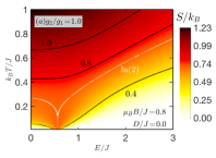
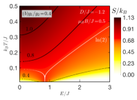
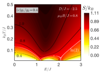
Figure 6: Density plots of the entropy in the electric field energy versus temperature plane for three selected sets of the model parameters in presence of an applied magnetic field. Displayed curves in all panels show isentropic lines, among which a particular isoline with $S/k_{B}\!=\!\ln(2)$ is highlighted by a white color.

In the range of magnetic fields, where the additional electric field leads to the electric-field driven phase transition (see Fig. 2) one can identify prolative infinitely fast change of temperature along the isoentropic line with $S/k_{B}\!=\!\ln(2)$. Consequently, the application of an additional electric field energy can enhance an observed MCE. Similarly as in the previously discussed MCE, the cooling temperature span can be tuned by variation of the strength of the single-ion anisotropy $D/J$ and/or the ratio of the Landé $g$-factors. Interestingly, there exists a parametric space, characterized through the existence of a triple point, where the increasing electric field can stimulate the cooling procedure with two consecutive cooling points located in a vicinity of the electric-field driven $|{\rm F}_{+}\rangle$-$|{\rm QF}_{-}\rangle$ and $|{\rm QF}_{-}\rangle$-$|{\rm QF}_{+}\rangle$ phase transitions (for an illustration see Fig. 6$(c)$). Based on the analysis of the ground-state phase diagram (Fig. 2) this parameter space is strongly conditioned by the strength of the single-ion anisotropy $D/J$, magnetic field $\mu_{B}B/J$ as well as the ratio $g_{2}/g_{1}$.

From the experimental point of view it is more advisable to analyze the isothermal entropy change $\Delta S_{T}^{M}$, an indirectly measured experimental quantity, defined as a difference of a magnetic entropy at non-zero and zero magnetic field at a fixed temperature

$$\Delta S_{T}^{M}(T,\mu_{B}\Delta B) \!=\!S_{2}(T,\mu_{B}B\!\neq\!0)-S_{1}(T,\mu_{B}B\!=\!0).$$ (29)

In such definition, the maximal magnitude of the isothermal entropy change $|\Delta S_{T}^{M}|$ corresponds to the maximal intensity of the MCE driven by an external field at a fixed temperature. It should be noted that in general, the isothermal entropy change $\Delta S_{T}^{M}$ can achieve both the positive as well as negative values, which characterize two different types of MCE. In the present convention $-\Delta S_{T}^{M}\!>\!0$ corresponds to the conventional MCE, whereas $-\Delta S_{T}^{M}\!<\!0$ is characteristic feature of a more exotic inverse MCE. The exact results obtained for the same model parameters as in Fig. 5 are presented in Fig. 7.

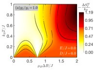
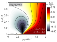
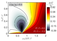
Figure 7: Density plots of the isothermal entropy change in the magnetic-field change versus temperature plane for three selected sets of model parameters in absence of an applied electric field. Displayed curves in all panels show isovalue lines running from $-\Delta S_{T}^{M}/k_{B}\!=\!-0.3$ to 1.2 with the step 0.1 (0.2) in a negative (positive) range.

For the fully isotropic case (Fig. 7$(a)$) only the conventional MCE is predicted for the whole range of magnetic field and temperature. The global maximum, and thus the most pronounced MCE, occurs approximately at relatively high temperature $k_{B}T/J\!\approx\!0.8$ at magnetic field where the $|{\rm F}_{+}\rangle$ ground state is favored. In the region of $|{\rm QF}_{+}\rangle$ ground state the maximal isothermal entropy change is gradually destroyed by thermal fluctuations. Naturally, the maximal thermal stability should be expected at the center of both transition points, where the impact of neighboring phases is minimal. Contrary to this, Figs. 7$(b)$ and 7$(c)$ indicate existence of both the conventional as well as inverse MCE in a certain region of the parameter space. The maximum of the conventional MCE is again detected at high-enough magnetic field but at significantly smaller temperature in comparison to the isotropic case. The inverse MCE is predicted at the proximity of the electric-field driven phase transition with a relatively low thermal stability depending on remaining model parameters. It should be emphasized, that the inverse MCE can arise in case of imbalanced Landé $g$-factors only.

Now let us look on the cross-section of the Fig. 7 to gain more insight into the behavior of the isothermal entropy change. The plots Fig. 8$(a)$ and $(b)$ illustrate the influence of the magnetic field on the isothermal entropy change $-\Delta S/k_{B}$ with an absence of electric field for fully isotropic case together with the other relevant quantity, the refrigerant capacity Pecharsky

$$Rc=\int_{T_{1}}^{T_{2}}\Delta S_{T}^{M}dT,$$ (30)

which allows us to calculate the performance of a refrigeration cycle and thus to quantify the amount of heat transferred between hot and cold reservoirs at temperatures $T_{1}$ and $T_{2}$. The limiting temperatures are selected as an intersection of integrated function and the constant function parallel to the $x$-axis passing through the half of maximal amplitude.

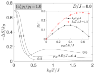
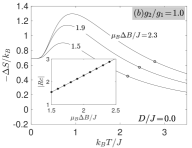
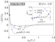
Figure 8: The dependence of a negative isothermal entropy change on the temperature for selected values of $\mu_{B}\Delta B/J$ and selected set of $D/J$, $g_{2}/g_{1}$ parameters. Open black and blue circles in main panels denote limiting temperatures emerging in the Eq. (30) to calculate the $|Rc|$ coefficient for the conventional MCE (CMCE) and inverse MCE (IMCE), respectively. Insets: The evolution of the $|Rc|$ coefficient under the external magnetic field span. Black (blue) curves illustrate the change of $Rc$ between $T_{1}$ and $T_{2}$ temperature for the conventional (inverse) MCE, while the red curve in the inset of panel $(a)$ illustrates the enlargement of $|Rc|$ if the upper fixed temperature limit, $k_{B}T_{2}/J\!=\!1.5$.

For the high-enough magnetic field, where the spontaneous $|{\rm F}_{+}\rangle$ phase is preferred (Fig. 8$(b)$) the isothermal entropy change is gradually enlarged with an increasing magnetic field. The magnitude as well as the position of maximum are also gradually enlarged. The refrigerant capacity (inset in Fig. 8$(b)$) clearly demonstrates an enhancement of the MCE driven by a magnetic field, which exhibits an expected linear character typical for the ferromagnetic phase. It should be emphasized, that the qualitatively identical behavior is detected for an arbitrary ratio $g_{2}/g_{1}$, if the $|{\rm F}_{+}\rangle$ ground state is realized. In the low-enough magnetic field, connected to the spontaneous $|{\rm QF}_{+}\rangle$ phase (Fig. 8$(a)$) the magnitude as well as the position of low-temperature maximum remains unchanged, while the width of maximum is varied upon the variation of magnetic field. The maximal isothermal entropy change is observed around the magnetic-field change $\mu_{B}\Delta B/J\!\sim\!0.4$ (black curve in the inset of Fig. 8$(a)$). Towards the one of the transition magnetic field, the interplay between the thermal fluctuations and the energy equivalence of both neighboring phases declines the heat transfer and thus the MCE decreases. Focusing on the higher (fixed) temperature interval (red curve in the inset of Fig. 8$(a)$) the refrigerant capacity can shift its maximum to the higher magnetic field as a consequence of the second broad maximum in the isothermal entropy change. The existence of an inverse MCE at finite temperatures gives rise to other extreme with an opposite sign. As illustrates Fig. 8$(c)$ the increasing magnetic field firstly enhances the magnitude of the isothermal entropy change reaching the maximum around the transition magnetic field. Subsequently, the negative minimum in isothermal entropy change vanishes similarly as the refrigerant capacity (blue dotted curve in the inset of Fig. 8$(c)$). On the other hand, the refrigerant capacity of the conventional MCE is minimal in the same region of $|{\rm QF}_{-}\rangle$ ground state, but rapidly enlarges when the transition point to the $|{\rm F}_{+}\rangle$ state is reached.

In an analogy to the isothermal entropy changes induced by the magnetic field we have similarly examined the isothermal entropy changes induced by the electric field energy characterizing the ECE at a certain magnetic field

$$\Delta S^{E}_{T}(T,\mu_{B}B,\Delta E) \!=\!S_{2}(T,\mu_{B}B,E\!\neq\!0)-S_{1}(T,\mu_{B}B,E\!=\!0).$$ (31)

A few illustrative examples of the isothermal entropy change are depicted in Fig. 9. It is quite clear that the MCE detected at $E/J\!=\!0.0$ can be significantly modulated in a proximity of electric-field-induced phase transitions $|{\rm F}_{+}\rangle$-$|{\rm QF}_{+}\rangle$ [Fig. 9$(a)$], $|{\rm QF}_{-}\rangle$-$|{\rm QF}_{+}\rangle$ [Fig. 9$(b)$] or both of them [Fig. 9$(c)$]. This fact can be convincingly evidenced through the positive isothermal entropy changes ($-\Delta S_{T}^{E}\!<\!0$) achieved upon variation of the electric field energy, which corroborate a possible existence of the inverse ECE. At each investigated case the global minimum, and thus the maximal inverse ECE, is detected exactly at the electric-field transition with the highest thermal stability, if a single electric-field driven phase transition takes place (Fig. 9$(a)$, $(b)$). In contradiction to this, the maximal temperature span of the inverse ECE in specific case with two consecutive critical points (Fig. 9$(c)$) lies in between both transition points. The most pronounced conventional ECE is evidenced at higher values of the electric field energy, but the Landé $g$-factor as well as the strength of the single-ion anisotropy significantly reduce the temperature of the ECE.

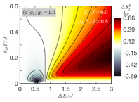
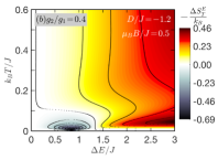
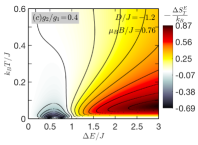
Figure 9: Density plots of the isothermal entropy change in the electric-field-change versus temperature plane for three selected sets of model parameters in presence of an applied magnetic field. Displayed curves in all panels show isovalue lines running from $-\Delta S_{T}^{E}/k_{B}\!=\!-0.7$ to 0.7 with the step 0.1.

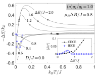
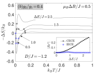
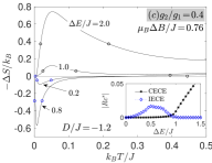
Figure 10: The dependence of a negative isothermal entropy change on the temperature for selected values of $\mu_{B}\Delta B/J$ and selected set of $D/J$, $g_{2}/g_{1}$ parameters. Open black and blue circles in main panels denote limiting temperatures emerging in the Eq. (30) to calculate the $|Rc|$ coefficient for the conventional ECE (CECE) and inverse ECE (IECE), respectively. Insets: The evolution of the $|Rc|$ coefficient under the external magnetic field span. Black (blue) curves illustrate the change of $Rc$ between $T_{1}$ and $T_{2}$ temperature for the conventional (inverse) ECE.

The cross-section of Fig. 9 clearly demonstrates that the increasing electric field energy in the region of $|{\rm QF}_{+}\rangle$ ground state significantly enhances the ECE with a motion of cooling temperature span to the higher value, see Fig. 10. In this case the magnitude of the isothermal entropy change enlarges due to the enhancement of the cooling temperature span ($-\Delta S\!>\!0$). Equally, the increment of the $Rc$ coefficient demonstrates the enhancement of the conventional ECE. Contrary to this, a sufficiently small value of electric field energy can enhance the inverse ECE, however the further increase of electric field energy completely reduces this nontrivial behavior. As a result, one can identify a very small maximum at $|Rc|$ behavior, see insets of Fig. 10. It is interesting to note, that in the parametric space with two consecutive electric-field transition points the $|Rc|$ coefficient of the inverse ECE involves two more or less visible maxima, because the highest heat transfer between reservoirs is realized in a close proximity of electric-field driven phase transition.

4 Conclusion

In the present paper we have rigorously examined the magnetocaloric and electrocaloric behavior of a mixed spin-(1/2, 1) Heisenberg dimer achieved upon variation of the external magnetic and electric fields. An exhaustive analysis of ground state points on existence of the field-driven phase transitions between the quantum ferrimagnetic phases $|{\rm QF}_{\pm}\rangle$ and the classical ferromagnetic phase $|{\rm F}_{+}\rangle$ depending basically on the uniaxial single-ion anisotropy $D/J$ and the ratio $g_{2}/g_{1}$ between Landé $g$-factors of both magnetic ions. It turns out that the difference of Landé $g$-factors generates an extraordinary behavior of the total magnetization and dielectric polarization with a pronounced quasi-plateau behavior. A mutual interaction between the magnetization and dielectric polarization serves in evidence of a magnetoelectric effect. A degeneracy accompanying zero-temperature phase transition driven either by the external magnetic or electric field causes an enhancement of the caloric effect. Three basic magnetocaloric characteristics, namely the isentropic changes of temperature, the isothermal entropy changes and the refrigerant capacity have been used to study the MCE and ECE in a wide range of the model parameters. It was found that the mixed spin-(1/2, 1) Heisenberg dimer may exhibit a conventional as well as inverse MCE in a proximity of magnetic-field-induced phase transitions. It was shown, furthermore, that existence of an inverse MCE is strictly conditioned by presence of the magnetic-field-driven phase transition between one of two quantum ferrimagnetic phases $|{\rm QF}_{\pm}\rangle$ and the fully polarized ferromagnetic phase $|{\rm F}_{+}\rangle$ under the assumption of the imbalanced ratio $g_{2}/g_{1}$ between Landé $g$-factors of constituent spins. The most interesting observation derived from our analysis is a possibility of enhancement of the MCE through a relative low-energy-consuming way, namely, an application of the external electric field. Utilizing the behavior of the refrigerant capacity it was demonstrated that the increasing electric field can significantly reduce the inverse ECE and can stabilize its conventional counterpart. As was shown furthermore, the conventional and inverse ECE in the mixed spin-(1/2, 1) Heisenberg dimer can be additionally tuned through the modulation of the magnetic field. Bearing all this in mind, the mixed spin-(1/2, 1) Heisenberg dimer represents a good theoretical tool for a rigorous study of unconventional multicaloric properties with a huge application potential.

Acknowledgments
This work was financially supported by the grant of the Slovak Research and Development Agency provided under the contract No. APVV-20-0150 and by the grant of The Ministry of Education, Science, Research, and Sport of the Slovak Republic and Slovak Academy of Sciences provided under the contract No. VEGA 1/0105/20.

Data Availability Statement
The data that support the findings of this study are available from the corresponding author upon reasonable request.

Conflict of interest
The authors declare that they have no known conflict of interest.

Appendix

The exact analytical expression of the partition function of the mixed spin-(1/2,1) Heisenberg dimer

$${\cal Z}\!=\!\sum_{i=1}^{6}{\rm e}^{-\beta\varepsilon_{i}}\!= 2\left\{\exp\left[-\frac{\beta}{2}(J+2D)\right]\cosh\left[\frac{\beta}{2}(h_{1}\!+\!2h_{2})\right]\right.\!+\!\exp\left[{\frac{\beta}{4}(J\!-\!2D)}\right]\left[\sum_{k=0,1}\exp\left[(-1)^{k}\frac{\beta h_{2}}{2}\right]\right.$$

$$\left.\times\!\cosh\!\left(\frac{\beta}{4}\sqrt{\left[J\!-\!2D\!-\!(-1)^{k}2(h_{1}\!-\!h_{2})\right]^{2}\!\!+\!8\left[(J\Delta)^{2}\!+\!E^{2}\right]}\right)\!\Bigg{]}\right\},$$ (32)

where $\beta\!=\!1/(k_{B}T)$, $k_{B}$ denotes the Boltzmann’s constant and $T$ is the absolute temperature.

The exact analytical expression of normalized magnetization derived from Eq. (18)

$$\frac{m}{m_{s}} \!=\!-\frac{\partial F}{\partial\mu_{B}B}\!=\!\frac{1}{\cal Z}\left\{\exp\left[-\frac{\beta}{2}(J\!+\!2D)\right](g_{1}\!+\!2g_{2})\sinh\left[\frac{\beta}{2}(h_{1}\!+\!2h_{2})\right]\!+\!\exp\left[\frac{\beta}{4}(J\!-\!2D)\right]\right.$$

$$\times\left[\exp\left(\frac{\beta h_{2}}{2}\right)\left(g_{2}\cosh\left[\frac{\beta}{4}\sqrt{\left[J\!-\!2D\!-\!2(h_{1}\!-\!h_{2})\right]^{2}\!+\!8\left[(J\Delta)^{2}\!+\!E^{2}\right]}\right]\right.\right.$$

$$\!-\!\left.\frac{(g_{1}\!-\!g_{2})(J\!-\!2D\!-\!2(h_{1}\!-\!h_{2}))}{\sqrt{\left[J\!-\!2D\!-\!2(h_{1}\!-\!h_{2})\right]^{2}\!+\!8\left[(J\Delta)^{2}\!+\!E^{2}\right]}}\sinh\left[\frac{\beta}{4}\sqrt{\left[J\!-\!2D\!-\!2(h_{1}\!-\!h_{2})\right]^{2}\!+\!8\left[(J\Delta)^{2}\!+\!E^{2}\right]}\right]\right)$$

$$\!-\!\exp\left(-\frac{\beta h_{2}}{2}\right)\left(g_{2}\cosh\left[\frac{\beta}{4}\sqrt{\left[J\!-\!2D\!+\!2(h_{1}\!-\!h_{2})\right]^{2}\!+\!8\left[(J\Delta)^{2}\!+\!E^{2}\right]}\right]\right.$$

$$\!-\!\left.\left.\left.\frac{(g_{1}\!-\!g_{2})(J\!-\!2D\!+\!2(h_{1}\!-\!h_{2}))}{\sqrt{\left[J\!-\!2D\!+\!2(h_{1}\!-\!h_{2})\right]^{2}\!+\!8\left[(J\Delta)^{2}\!+\!E^{2}\right]}}\sinh\left[\frac{\beta}{4}\sqrt{\left[J\!-\!2D\!+\!2(h_{1}\!-\!h_{2})\right]^{2}\!+\!8\left[(J\Delta)^{2}\!+\!E^{2}\right]}\right]\right)\right]\right\}.$$ (33)

The exact analytical expression of the dimensionless dielectric polarization derived from Eq. (19)

$$P\! =\!-{\mu}\frac{\partial F}{\partial E}\!=\!\frac{4E}{\cal Z}\exp\left[\frac{\beta}{4}(J\!-\!2D)\right]\left\{\exp\left(\frac{\beta h_{2}}{2}\right)\frac{\sinh\left[\frac{\beta}{4}\sqrt{\left[J\!-\!2D\!-\!2(h_{1}\!-\!h_{2})\right]^{2}\!+\!8\left[(J\Delta)^{2}\!+\!E^{2}\right]}\right]}{\sqrt{\left[J\!-\!2D\!-\!2(h_{1}\!-\!h_{2})\right]^{2}\!+\!8\left[(J\Delta)^{2}\!+\!E^{2}\right]}}\right.$$

$$\!+\!\left.\exp\left(-\frac{\beta h_{2}}{2}\right)\frac{\sinh\left[\frac{\beta}{4}\sqrt{\left[J\!-\!2D\!+\!2(h_{1}\!-\!h_{2})\right]^{2}\!+\!8\left[(J\Delta)^{2}\!+\!E^{2}\right]}\right]}{\sqrt{\left[J\!-\!2D\!+\!2(h_{1}\!-\!h_{2})\right]^{2}\!+\!8\left[(J\Delta)^{2}\!+\!E^{2}\right]}}\right\}.$$ (34)

Finally, the explicit analytical expression of the entropy satisfies the Eq. (20)

$$\displaystyle S =-\frac{\partial F}{\partial T}\!=\!k_{B}\ln{\cal Z}\!+\!\frac{1}{T{\cal Z}}\left\{\exp\left[-\frac{\beta}{2}(J\!+\!2D)\right]\left[\left(J\!+\!2D\right)\cosh\left[\frac{\beta}{2}(h_{1}\!+\!2h_{2})\right]\!-\!(h_{1}\!+\!2h_{2})\sinh\left[\frac{\beta}{2}(h_{1}\!+\!2h_{2})\right]\right]\right.$$

$$-\frac{1}{2}\exp\left[\frac{\beta}{4}(J\!-\!2D)\right]\left[\exp\left(\frac{\beta h_{2}}{2}\right)\Bigg{(}(J\!-\!2D\!+\!2h_{2})\cosh\left(\frac{\beta}{4}\sqrt{\left[J\!-\!2D\!-\!2(h_{1}\!-\!h_{2})\right]^{2}\!+\!8\left[(J\Delta)^{2}\!+\!E^{2}\right]}\right)\right.$$

$$+\sqrt{\left[J\!-\!2D\!-\!2(h_{1}\!-\!h_{2})\right]^{2}\!+\!8\left[(J\Delta)^{2}\!+\!E^{2}\right]}\sinh\left(\frac{\beta}{4}\sqrt{\left[J\!-\!2D\!-\!2(h_{1}\!-\!h_{2})\right]^{2}\!+\!8\left[(J\Delta)^{2}\!+\!E^{2}\right]}\right)\Bigg{)}$$

$$+\exp\left(-\frac{\beta h_{2}}{2}\right)\Bigg{(}(J\!-\!2D\!-\!2h_{2})\cosh\left(\frac{\beta}{4}\sqrt{\left[J\!-\!2D\!+\!2(h_{1}\!-\!h_{2})\right]^{2}\!+\!8\left[(J\Delta)^{2}\!+\!E^{2}\right]}\right)$$

$$\left.\left.+\sqrt{\left[J\!-\!2D\!+\!2(h_{1}\!-\!h_{2})\right]^{2}\!+\!8\left[(J\Delta)^{2}\!+\!E^{2}\right]}\sinh\left(\frac{\beta}{4}\sqrt{\left[J\!-\!2D\!+\!2(h_{1}\!-\!h_{2})\right]^{2}\!+\!8\left[(J\Delta)^{2}\!+\!E^{2}\right]}\right)\Bigg{)}\right]\right\}\;.$$ (35)

References

- (1) W. K. Wootters, Quantum Inform. Comput. 1 (2001) 27.
- (2) A. M. Souza, M. S. Reis, D. O. Soares-Pinto, I. S. Oliveira, and R. S. Sarthour, Phys. Rev. B 77 (2008) 104402.
- (3) R. Horodecki, P. Horodecki, M. Horodecki, and K. Horodecki, Rev. Mod. Phys. 81 (2009) 865.
- (4) O. Rojas, M. Rojas, N. S. Ananikian, and S. M. de Souza, Phys. Rev. A 86 (2012) 042330.
- (5) H. Čenčariková and J. Strečka, Phys. Rev. B 102 (2020) 184419.
- (6) H. Vargová and J. Strečka, Phys. Nanomaterials 11 (2021) 3096.
- (7) H. Vargová, J. Strečka, and N. Tomašovičová, J. Magn. Magn. Mater. 546 (2022) 168799.
- (8) A. Honecker, J. Schulenburg, and J. Richter, J. Phys.: Condens. Matter 16 (2004) S749.
- (9) V. Ohanyan, O. Rojas, J. Strečka, and S. Bellucci, Phys. Rev. B 92 (2015) 214423.
- (10) H. Čenčariková, J. Strečka, and A. Gendiar, J. Magn. Magn. Mater. 452 (2018) 512.
- (11) Introduction to Frustrated Magnetism, edited by C. Lacroix, Ph. Mendels, and F. Mila (Springer, Heidelberg, 2011).
- (12) A. Imambekov, T. L. Schmidt, and L. I. Glazman, Rev. Mod. Phys. 84 (2012)1253.
- (13) J. W. Sharples, D. Collison, E. J. L. McInnes, J. Schnack, E. Palacios, and M. Evangelisti, Nat. Commun. 5 (2014) 5321.
- (14) O. Baran, V. Ohanyan, and T. Verkholyak, Phys. Rev. B 98 (2018) 064415.
- (15) H. Čenčariková and J. Strečka, Phys. Rev. E 98 (2018) 062129.
- (16) V. Ohanyan, Condens. Matter. Phys. 23 (2020) 43704.
- (17) D. Markham and B. C. Sanders, Phys. Rev. A 78 (2008) 042309.
- (18) W. Matthews, S. Wehner, and A. Winter, Commun. Math. Phys. 291 (2009) 813.
- (19) R. Rahaman and M. G. Parker, Phys. Rev. A 91 (2015) 022330.
- (20) Z. Fu, Y. Xiao, Y. Su, Y. Zheng, P. Kögerler, and T. Brückel, EPL 112 (2015) 27003.
- (21) N. A. de Oliveira and P. J. von Ranke, Phys. Rep. 489 (2010) 89.
- (22) J. Torrico, M. Rojas, S. M. de Souza, and O. Rojas, Phys. Lett. A 380 (2016) 3655.
- (23) P. Kowalewska and K. Szałowski, J. Magn. Magn. Mater 496 (2020) 165933.
- (24) A. S. Mischenko, Q. Zhang, J. F. Scott, R. W. Whatmore, and N. D. Mathur, Science 311 (2006), 1270.
- (25) X. Moya, S. Kar-Narayan, and N. D. Mathur, Nat. Mater. 13 (2014), 439.
- (26) K. Szałowski and T. Balcerzak, Sci. Rep. 8 (2018) 5116.
- (27) J. Glanz, Science 279 (1998) 2045.
- (28) M. Ismail, M. Yebiyo, and I. Chaer, Energies 14 (2021) 502.
- (29) H. Ursic, V. Bobnar, B. Malic, C. Filipic, M. Vrabelj, S. Drnovske, Y. Jo, M. Wencka, and Z. Kutnjak, Sci. Rep. 6 (2016) 26629.
- (30) K. Qiao, S. Zuo, H. Zhang, F. Hu, Z. Yu, F. Weng, Y. Liang, H. Zhou, Y. Long, J. Wang, J. Sun, T. Zhao, and B. Shen, Scr. Mater. 204 (2021) 114141.
- (31) K. Szałowski and T. Balcerzak, J. Magn. Magn. Mater. 527 (2021) 167767.
- (32) H. A. Zad, M. Sabeti, A. Zoshki, and N. Ananikian, J. Phys.: Condens. Matter 31 (2019) 425801.
- (33) L. J. Ding and Y. Zhong, Phys. Chem. Chem. Phys. 20 (2018) 20228.
- (34) J. Richter, V. Ohanyan, J. Schulenburg, and J. Schnack, arxiv:2107.04371v1.
- (35) F.K. Fodouop, G.C. Fouokeng, A.T. Tsokeng, M. Tchoffo, and L.C. Fai, Physica E 128 (2021) 114616.
- (36) P. J. von Ranke, M. A. Mota, D. F. Grangeia, A. M. G. Carvalho, F. C. G. Gandra, A. A. Coelho, A. Caldas, N. A. de Oliveira, and S. Gama, Phys. Rev. B 70 (2004) 134428.
- (37) T. Krenke, E. Duman, M. Acet, E. F. Wassermann, X. Moya, L. Manosa, and A. Planes, Nat. Mater. 4 (2005) 450.
- (38) T. Krenke, M. Acet, E. F. Wassermann, X. Moya, L. Manosa, and A. Planes, Phys. Rev. B 72 (2005) 014412.
- (39) K. G. Sandeman, R. Daou, S.Özcan, J. H. Durrell, N. D. Mathur, and D. J. Fray, Phys. Rev. B 74 (2006) 184412.
- (40) A.K. Nayak, M. Nicklas, S. Chadov, P. Khuntia, Ch. Shekhar, A. Kalache, M. Baenitz, Y. Skourski, V. K. Guduru, A. Puri, U. Zeitler, J. M. D. Coey, and C. Felser, Nat. Mater. 14 (2015) 679.
- (41) A. Biswas, S. Chandra, T. Samanta, M. H. Phan, I. Das, and H. Srikanth, J. Appl. Phys. 113 (2013) 17A902.
- (42) S. Uddin, G.-P. Zheng, Y. Iqbal, R. Ubic, and J. Yang, J. Appl. Phys.14 (2013) 213519.
- (43) W. Geng, Y. Liu, X. Meng, L. Bellaiche, J. F. Scott, B. Dkhil, and A. Jiang, Adv. Mater. 27 (2015) 3165.
- (44) J. Peräntie, J. Hagberg, A. Uusimäki, and H. Jantunen, Phys. Rev. B 82 (2010) 134119.
- (45) F. Le Goupil, A. Berenov, A.-K. Axelsson, M. Valant, and N. McN. Alford, J. Appl. Phys. 111 (2012) 124109.
- (46) O. Derzhko and J. Richter, Eur. Phys. J. B 52 (2006) 23.
- (47) M. S. S Pereira, F. A. B. F. de Moura, and M. M. Lyra, Phys. Rev. B 79 (2009) 054427.
- (48) T. Verkholyak and J. Strečka, Phys. Rev. B 88 (2013) 134419.
- (49) K. Szałowski and T. Balcerzak, J. Phys.: Condens. Matter 26 (2014) 386003.
- (50) L. Gálisová and J. Strečka, Phys. Rev. E 91 (2015) 022134.
- (51) C. Krishnamoorthi, S. K. Barik, Z. Siu, and R. Mahendiran, Sol. Stat. Commun. 150 (2010) 1670.
- (52) L. V. B. Diop and O. Isnard, J. Appl. Phys. 119 (2016) 213904.
- (53) T. Odaira, S. Xu, X. Xu, T. Omori, and R. Kainuma, Appl. Phys. Rev. 7 (2020) 031406.
- (54) E. Burzo, I. Balacz, I Deac, and R. Tetean, J. Magn. Magn. Mater. 322 (2010) 1109.
- (55) Q. Zhang, F. Guillou, A. Wahl, Y. Brard, and V. Hardy, Appl. Phys. Lett. 96 (2010) 242506.
- (56) R. D. dos Reis, L. M. de Silva, A. O. dos Santos, A. M. N. Medina, L. P. Carloso, and F. G. Fandra, J. Phys.: Condens. Matter 22 (2010) 486002.
- (57) D. Gatteschi, R. Sessoli, and J. Villain, Molecular Nanomagnets, Oxford University Press, Oxford, 2006.
- (58) O, Kahn, Molecular Magnetism, VCH Publishers, New York, 1993.
- (59) Y. Hieida, K. Okunishi, and Y. Akutsu, Phys. Rev. B 64 (2001) 224422.
- (60) D.V. Dmitriev and K.V. Ya, Phys. Rev. B 70 (2004) 144414.
- (61) T. Hikihara and A. Furusaki, Phys. Rev. B 69 (2004) 064427.
- (62) R. Hagemans, J.-S. Caux, and U. Low, Phys. Rev. B 71 (2005) 014437.
- (63) J.-S. Caux, F.H.L. Essler, and U. Low, Phys. Rev. B 68 (2003) 134431.
- (64) O. Menchyshyn, V. Ohanyan, T. Verkholyak, T. Krokhmalskii, and O. Derzhko, Phys. Rev. B 92 (2015) 184427.
- (65) M. Brockmann, A. Klümper, and V. Ohanyan, Phys. Rev. B 87 (2013) 054407.
- (66) S. Chen, H. Buttner, and J. Voit, Phys. Rev. B 67 (2003) 054412.
- (67) O. L. Bacq, A. Pasturel, C. Lacroix, and M. D. N. Regueiro, Phys. Rev. B 71 (2005) 014432.
- (68) B. Gu and G. Su, Phys. Rev. B 75 ( 2007) 174437.
- (69) N. B. Ivanov, Condens. Matter. Phys. 12 (2009) 435.
- (70) O. Rojas, M. Rojas, S. M. D. Souza, J. Torrico, J. Strečka, and M. L. Lyra, Physica A 486 (2017) 367.
- (71) O. Rojas, J. Strečka, M. L. Lyra, and S. M. de Souza, Phys. Rev. E 99 (2019) 042117.
- (72) J. Strečka, L. Gálisová, and T. Verkholyak, Phys. Rev. E 101 (2020) 012103.
- (73) A. Furrer and O. Waldmann, Rev. Mod. Phys. 85 (2013) 367.
- (74) J. T. Haraldsen, T. Barnes, and J. L. Musfeldt, Phys. Rev. B 71 (2005) 064403.
- (75) D. V. Efremov and R. A. Klemm, Phys. Rev. B 66 (2002) 174427.
- (76) M.-H. Whangbo, H.-J. Koo, and D. Dai, J. Sol. Stat. Chem. 176 (2003) 417.
- (77) A. Gleizes and M. Verdaguer, J. Am. Chem. Soc. 103 (1984) 7373.
- (78) M. Hagiwara, K. Minami, Y. Narumi, K. Tatani, and K. Kindo, J. Phys. Soc. Jap. 67 (1998) 2209.
- (79) P. J. van Koningsbruggen, O. Kahn, K. Nakatani, Y. Pei, J. P. Renard, M. Drillon, and P. Legoll, Inorg. Chem 29 (1990) 3325.
- (80) M. Hagiwara, Y. Narumi, K. Minami, K. Tatani, and K. Kindo, J. Phys. Soc. Jap. 68 (1999) 2214.
- (81) Y. Pei, M. Verdaquer, O. Kahn, J. Sletten, and J. P. Renard, Inorg. Chem. 26 (1987) 138.
- (82) G. Houchins and J. T. Haraldsen, Phys. Rev. B 91 (2015) 014422.
- (83) H. Katsura, N. Nagaosa, and A. V. Balatsky, Phys. Rev. Lett. 95 (2005) 057205.
- (84) C. Jia, S. Onoda, N. Nagaosa, and J. H. Han, Phys. Rev. B 74 (2006) 224444.
- (85) V. K. Pecharsky and K. A. Gschneidner, J. Appl. Phys. 90 (2001) 4614.