Mean Back Relaxation for Position and Densities

Abstract

Correlation functions are a standard tool for analyzing statistical particle trajectories. Recently, a so called mean back relaxation (MBR) has been introduced, which correlates positions at three time points and which has been shown to be a marker for breakage of time reversal symmetry for confined particles. Here, we extend this discussion in several ways. We give an extension to multiple dimensions. Using a path integral approach, we provide a general expression for MBR in terms of multipoint density correlations. For Gaussian systems, this expression yields a relation between MBR and mean squared displacement. From it, several properties of MBR for Gaussian equilibrium systems can be found, such as monotonicity and positivity. Unexpectedly, in this case the particle forgets the conditioning via a power law in time. We finally demonstrate that using MBR for microscopic densities, it is a marker for broken detailed balance even in bulk systems.

I Introduction

The analysis of particle trajectories is a fundamental building block of modern statistical physics, both in simulation and experiment. Especially in the latter, nowadays advanced techniques allow particle tracking with high precision and time resolution, leading to an extensive use of statistical analysis and the determination of microrheological and non-equilibrium properties of complex media [1, 2, 3, 4, 5]. Correlation functions obtained from these trajectories, like the mean squared displacement (MSD), are in equilibrium related to powerful theorems like the fluctuation dissipation theorem (FDT) or Green-Kubo relation [6, 7, 8, 9, 10, 11]. Breakage of time reversal symmetry is quantified by entropy production, for which powerful theorems exist [12, 13, 14, 15, 16, 17, 18, 19]. Notably, the MSD is not able to detect the breakage of time reversibility, and is thus unrelated to entropy production. On the other hand, multi-point correlation functions, that depend on multiple time points, have the potential to be sensitive to time reversal breakage and can therefore serve as intriguing observables in non-equilibrium systems. Conditioning trajectories, for example by selecting trajectories that start at certain positions [20, 21, 22] has lead to interesting insights. In the following, we will analyze a multi-point observable that has been termed mean back relaxation (MBR) [23, 24]. It was shown that MBR is a marker for broken detailed balance in confinement [23]. In this manuscript we expand on the properties of this quantity and analyze it in more depth. We also extend it towards the microscopic densities, which yields a marker for broken detailed balance even for bulk systems.

The manuscript is organized as follows. In section II, we define the MBR as an example for conditioned correlation and first discuss its properties in confined systems in section III. We reproduce the proof that the MBR is a non-equilibrium marker in confinement, summarized in a fluctuation theorem. We probe these findings on active Brownian particles trapped in a potential. In section IV we provide an analytic result for MBR in a system of $N$ coupled overdamped particles, which allows to discuss the properties of the MBR when obtained from the projected dynamics of a single particle. In sections V and VI, we derive conditioned correlations in a path integral formalism and apply this to find a general solution for the MBR in Gaussian systems in terms of the mean squared displacement, in one and multiple dimensions. At last in section VII we introduce a new version of the MBR based on densities, showing that it acts as a marker for broken detailed balance in bulk systems and confinement.

II Conditioned correlations exemplified at the Mean Back Relaxation

The mean back relaxation (MBR) [23] is the average future displacement of a particle under the condition of a displacement in the past. In one dimension, we define it in terms of two time periods $t$ and $\tau$, as,

$$\begin{split}\mathcal{M}(\tau,t)=\int\text{d}x_{t}\text{d}x_{0}\text{d}x_{-\tau}\left(-\frac{x_{t}-x_{0}}{x_{0}-x_{-\tau}}\right)\times\\ \times W_{3}(x_{t},t;x_{0},0;x_{-\tau},-\tau).\end{split}$$ (1)

$W_{3}$ is the three point probability function, i.e., the probability of finding a particle at the positions $x_{t},x_{0},x_{-\tau}$ at the corresponding times. The MBR is thus the ratio of the displacement $b=x_{t}-x_{0}$ in future, i.e., between $t$ and $0$ and the displacement in the past, $d=x_{0}-x_{-\tau}$, i.e., between times $-\tau$ and 0. $b$ and $d$ have typically opposite signs [23], because the particle travels in the opposite direction or relaxes back compared to its earlier movement. We therefore include by convention a minus sign, which will render the MBR positive in equilibrium, as will be shown below. We also note that MBR in Ref. [23] was defined as the limit of $\tau\to 0$ of the above expresssion. To illustrate the meaning of a conditioned mean, we give the following equivalent formulation

$$\begin{split}\mathcal{M}(\tau,t)&=\int\text{d}d\text{d}b\left(-\frac{b}{d}\right)p(b,d)\\ &=\int\text{d}d\left(-\frac{\left\langle b\right\rangle_{|d}}{d}\right)p(d).\end{split}$$ (2)

Here $\left\langle b\right\rangle_{|d}=\left\langle x_{t}-x_{0}\right\rangle_{|d}=\int\text{d}b\leavevmode\nobreak\ [b\leavevmode\nobreak\ p(b|d)]$ is the conditional average of the displacement $b=x_{t}-x_{0}$ given $d$. Eq. (2) shows that MBR probes how conditions affect the movement of the particle. Division by $d$ in the equations above renders MBR dimensionless. It also yields a cancellation of the signs of $b$ and $d$, so that displacements in either directions contribute equally.

While mostly focusing on a one dimensional observable, we will in section VI.4 provide results for the case of multiple dimensions, where different components of past and future displacements may be considered. This yields an MBR matrix,

$$\begin{split}{\mathcal{M}}_{ij}(\tau,t)=\int\text{d}^{n}\mathbf{x}_{t}\text{d}^{n}\mathbf{x}_{0}\text{d}^{n}\mathbf{x}_{-\tau}\left(-\frac{x^{(i)}_{t}-{x}^{(i)}_{0}}{x^{(j)}_{0}-{x}^{(j)}_{-\tau}}\right)\times\\ \times W_{3}(\mathbf{x}_{t},t;\mathbf{x}_{0},0;\mathbf{x}_{-\tau},-\tau).\end{split}$$ (3)

Here, $x^{(i)}$ is the $i$ component of the particle position, but the index may naturally also run over different particles.

III MBR in confinement

III.1 Long time limit of MBR and time reversal

In this subsection, we reproduce, for completeness, the results given in [23] for MBR. In a confined system with ergodicity, a well-defined mean position $\left\langle x\right\rangle=\int\text{d}x\leavevmode\nobreak\ x\leavevmode\nobreak\ p_{\text{stat}}(x)$ exists, corresponding to a well-defined stationary distribution $p_{\text{stat}}(x)$. If we assume finite correlation times, the joint three-point distribution function can be separated for large times $t$,

$$\begin{split}\lim_{t\to\infty}&W_{3}(x_{t},t;x_{0},0;x_{-\tau},-\tau)\\ &=p_{\text{stat}}(x_{t})W_{2}(x_{0},0;x_{-\tau},-\tau).\end{split}$$ (4)

We introduced the joint two-point probability $W_{2}$. Eq. (4) assumes that for large times $t$ the position $x_{t}$ is independent of $x_{0}$ and $x_{-\tau}$. We can insert these findings into the definition of the MBR Eq. (1)

$$\lim_{t\to\infty}\mathcal{M}(\tau,t) =\int\text{d}x_{t}\text{d}x_{0}\text{d}x_{-\tau}\left(-\frac{x_{t}-x_{0}}{x_{0}-x_{-\tau}}\right)\times$$ (5)

$$\leavevmode\nobreak\ \leavevmode\nobreak\ \leavevmode\nobreak\ \times p_{\text{stat}}(x_{t})W_{2}(x_{0},0;x_{-\tau},-\tau)$$

$$=\int\text{d}x_{0}\text{d}x_{-\tau}\left(-\frac{\left\langle x\right\rangle-x_{0}}{x_{0}-x_{-\tau}}\right)\times$$ (6)

$$\leavevmode\nobreak\ \leavevmode\nobreak\ \leavevmode\nobreak\ \times W_{2}(x_{0},0;x_{-\tau},-\tau)$$

with $\left\langle x\right\rangle=\int\text{d}x\leavevmode\nobreak\ x\leavevmode\nobreak\ p_{\text{stat}}(x)$ that mean position of the stationary distribution. Under time reversal the position $x_{0}$ and $x_{-\tau}$ of the long-time value of MBR are exchanged. The long-time value can therefore be rewritten as

$$\lim_{t\to\infty} \mathcal{M}(\tau,t)=\frac{1}{2}+\frac{1}{2}\int\text{d}x_{0}\text{d}x_{-\tau}\left(-\frac{\left\langle x\right\rangle-x_{0}}{x_{0}-x_{-\tau}}\right)\times$$ (7)

$$\times\left[W_{2}(x_{0},0;x_{-\tau},-\tau)-W_{2}(x_{-\tau},0;x_{0},-\tau)\right]$$

$$=\frac{1}{2}+\frac{1}{2}\left\langle\frac{(x_{0}-\left\langle x\right\rangle)+(x_{-\tau}-\left\langle x\right\rangle)}{x_{0}-x_{-\tau}}\right\rangle,$$ (8)

i.e., as a sum of a part symmetric under time reversal and an anti-symmetric part $\frac{1}{2}\frac{(x_{0}-\left\langle x\right\rangle)+(x_{-\tau}-\left\langle x\right\rangle)}{x_{0}-x_{-\tau}}$. The latter changes sign when the MBR is evaluated for the reversed trajectory. If a system is in equilibrium, hence detailed balance is fulfilld, i.e., $p[x(t)]=p[\theta x(t)]$, the average of any anti-symmetric observable vanishes. We introduced the path probability $p[x(t)]$, with bracket $[\dots]$ indicating the functional dependence on $x(t)$. The time reversal operator $\theta x(t)=x(t_{\text{end}}-t)$ reverses a trajectory and reverses all momenta. The above argument show that, with detailed balance fulfilled,

$$\lim_{t\to\infty}\mathcal{M}(\tau,t)\overset{db.}{=}\frac{1}{2}$$ (9)

independent of the dynamics and the time period $\tau$.

We will now derive a fluctuation theorem for MBR, for which we introduce the stochastic total change of entropy defined as[25, 26, 13]

$$s\left[x(t)\right]=\log\frac{p[x(t)]}{p[\theta x(t)]}.$$ (10)

Stochastic total change of entropy therefore compares the probability of a given path to the probability of its reversed. Eq. (8) is reformulated in the fluctuation theorem [19]

$$\left\langle\left(-\frac{\left\langle x\right\rangle-x_{0}}{x_{0}-x_{-\tau}}\right)\left(1+e^{-s}\right)\right\rangle=1.$$ (11)

Note that for any observable $O(x(t))$ the average of the time reversed observable can be rewritten as

$$\left\langle O[\theta x(t)]\right\rangle =\int\mathcal{D}x(t)O[x(t)]\frac{p[\theta x(t)]}{p[x(t)]}p[x(t)]$$ (12)

$$=\left\langle O[x(t)]e^{-s}\right\rangle$$ (13)

using entropy production as defined in Eq. (10) and $\mathcal{D}x(t)$ denoting a path integral. The fluctuation theorem Eq. (11) therefore states that the long-time value of normal and reversed dynamics, always add up to one

$$\begin{split}\lim_{t\to\infty}&\left(\mathcal{M}(\tau,t)+\mathcal{M}_{r}(\tau,t)\right)\\ &=\left\langle-\frac{\left\langle x\right\rangle-x_{0}}{x_{0}-x_{-\tau}}-\frac{\left\langle x\right\rangle-x_{-\tau}}{x_{-\tau}-x_{0}}\right\rangle=1,\end{split}$$ (14)

where we introduced $\mathcal{M}_{r}(\tau,t)$ as MBR evaluated from time backward trajectories. In equilibrium normal and revered dynamics are statistically indistinguishable, which is equivalent to $s=0$ for all paths, hence the long-time value of the MBR equals $\frac{1}{2}$ as stated previously.

To sum up, in a confined system the long-time value of the MBR in equilibrium universally equals $\frac{1}{2}$. With detailed balance broken, MBR may differ from $\frac{1}{2}$ but the long-time values of normal and reversed dynamics always have to add up to one. A deviation from $\frac{1}{2}$ thus marks non-equilibrium. These results are summarized in the MBR fluctuation theorem Eq. (11).

III.2 Example: Active Brownian particles

To demonstrate the results of the previous subsection, we probe a two-dimensional active Brownian particle confined in a harmonic trap of stiffness $k$, described by the Langevin equations [27, 28]

$$\dot{\mathbf{x}} =-\frac{k}{\gamma}\mathbf{x}+v_{0}\mathbf{\hat{e}}(\varphi)+\mathbf{f}$$ (15a)

$$\dot{\varphi} =f_{\varphi}$$ (15b)

with $\mathbf{\hat{e}}=(\cos(\varphi),\sin(\varphi))^{\intercal}$, white noise random forces $\left\langle f^{(i)}(t)f^{(j)}(t^{\prime})\right\rangle=2D\delta(t-t^{\prime})\delta_{ij}$ and $\left\langle f_{\varphi}(t)f_{\varphi}(t^{\prime})\right\rangle=2D_{\varphi}\delta(t-t^{\prime})$. Simulation results are shown in Fig. 1, where we use one of the coordinates to evaluate MBR. If the active propulsion $v_{0}=0$ vanishes, the system is in equilibrium. The blue line in Fig. 1(a) shows this case, and indeed MBR approaches the equilibrium $\frac{1}{2}$ value. (b) shows the long-time value for different $\tau$ where it is visible that this feature is independent of $\tau$.

The red lines in Figure 1 are for finite $v_{0}$. In this case the long-time MBR deviates from $\frac{1}{2}$, indicating non-equilibrium. Further this effect is most pronounced for a specific $\tau$ and vanishes for $\tau\to\infty$. Evaluation of the MBR for the reversed trajectories results in a deviation of the long-time value in the opposite direction of $\frac{1}{2}$, i.e., they add up to one as stated by the fluctuation theorem Eq. (11). The active Brownian particles therefore demonstrate that the MBR can detect the breakage of time reversal symmetry, and this breakage is accurately described by the corresponding fluctuation theorem.

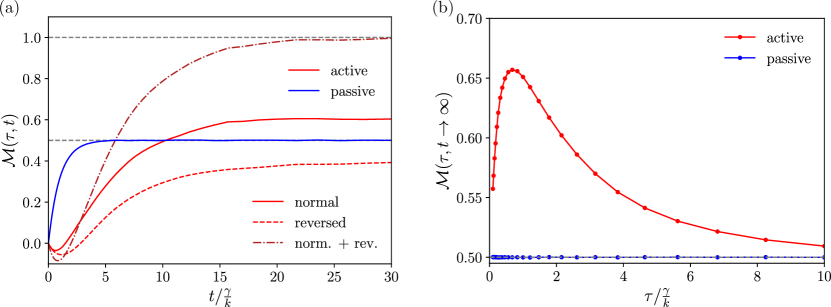
Figure 1: MBR curves obtained from simulations of active Brownian particles defined according to Eq. (15). (a) shows MBR as a function of time in units of $\frac{\gamma}{k}$ for $\tau=2\frac{\gamma}{k}$ and $\frac{D_{\varphi}}{\beta kD}=0.2$, the blue line shows a particle $v_{0}=0$ which corresponds to equilibrium, and MBR approaches the long-time value $\frac{1}{2}$. The solid red lines are active Brownian particles with $\frac{v_{0}}{\sqrt{\beta k}D}=7$. The long-time value deviates from $\frac{1}{2}$, indicating a non-equilibrium system. The red dotted line is the same system, however, the MBR is evaluated for the reversed trajectories. In this case the MBR deviates from $\frac{1}{2}$ in opposite direction. Their sum is shown as a dark red dotted line, which approaches unity in the long-time limit, as predicted by the fluctuation theorem Eq.(11). (b) shows the long-time limit of the MBR as function of $\tau$. In the passive case $v_{0}=0$ (blue line) the MBR is $\frac{1}{2}$ independent of $\tau$. In the active case $\frac{v_{0}}{\sqrt{\beta k}D}=7$ the deviation increases with $\tau$, until it hits a maximum and decreases afterwards to $\frac{1}{2}$.

IV MBR in bulk: Insights from a linear model system

In a bulk system, one cannot expect $\left\langle x\right\rangle$ to exist, and the derivations in section III are not valid. Nevertheless, the MBR has interesting properties in bulk as well, which we exemplify with a system of coupled particles. Consider the following set of $N$ linear Langevin equations, describing harmonically coupled overdamped particles

$$\dot{x}^{(i)}=\frac{1}{\gamma_{i}}\sum_{j}\left(-k_{ij}(x^{(i)}-x^{(j)})\right)+f^{(i)},$$ (16)

with $\left\langle f^{(i)}(t)f^{(j)}(t)\right\rangle=\frac{2k_{B}T_{i}}{\gamma_{i}}\delta(t-t^{\prime})\delta_{ij}$, with friction coefficients $\gamma_{i}$, temperatures $T_{i}$ and coupling constant $k_{ij}>0$ which are symmetric in the components $k_{ij}=k_{ji}$ and $k_{ii}=0$. We thus exclude here external potentials (for confining potentials, the stronger statements of section III apply). To allow for equilibrium as well as out of equilibrium conditions, we include the possibility of different particle temperatures $T_{i}$. Such a system of equations can be decomposed into a center coordinate $x_{s}$ and relative coordinates. The center is defined as $x_{s}=\frac{\sum_{i=1}^{N}\gamma_{i}x^{(i)}}{\sum_{i=1}^{N}\gamma_{i}}$ and it follows the Langevin equation

$$\dot{x}_{s}=f_{s}$$ (17)

with white noise $\left\langle f_{s}(t)f_{s}(t^{\prime})\right\rangle=\frac{2k_{B}}{\Gamma^{2}}\sum_{i=1}^{N}T_{i}\gamma_{i}\delta(t-t^{\prime})$ and $\Gamma=\sum_{i=1}^{N}\gamma_{i}$. Every particle is thus expressed by its position relative to it $x^{(i)}-x_{s}=\frac{\sum_{j=1}^{N}\gamma_{j}(x^{(i)}-x^{(j)})}{\Gamma}$. Because the variables $\left\langle x^{(i)}-x^{(j)}\right\rangle=0$ are centered, the mean position of one particle $x^{(i)}$

$$\left\langle x^{(i)}\right\rangle=\left\langle x_{s}\right\rangle+\frac{\sum_{j=1}^{N}\gamma_{j}\left\langle x^{(i)}-x^{(j)}\right\rangle}{\Gamma}=\left\langle x_{s}\right\rangle$$ (18)

equals the mean of the center coordinate. Using this insight we can revisit Eq. (III.1) and find in the limit of large time $t$ for the MBR of one of the particles (say particle 1, $x^{(1)}$)

$$\lim_{t\to\infty}\mathcal{M}(\tau,t) =\int\text{d}x^{(1)}_{0}\text{d}x^{(1)}_{-\tau}\left(-\frac{\left\langle x_{s}\right\rangle-x^{(1)}_{0}}{x^{(1)}_{0}-x^{(1)}_{-\tau}}\right)\times$$

$$\leavevmode\nobreak\ \leavevmode\nobreak\ \leavevmode\nobreak\ \times W_{2}(x^{(1)}_{0},0;x^{(1)}_{-\tau},-\tau)$$

$$=\int\prod_{i=1}^{N}\text{d}x_{0}^{(i)}\text{d}x_{-\tau}^{(i)}\times$$

$$\leavevmode\nobreak\ \leavevmode\nobreak\ \leavevmode\nobreak\ \times\left(-\frac{1}{\Gamma}\frac{\sum_{i=1}^{N}\gamma_{i}x_{0}^{(i)}-\Gamma x_{0}^{(1)}}{x^{(1)}_{0}-x^{(1)}_{-\tau}}\right)\times$$

$$\leavevmode\nobreak\ \leavevmode\nobreak\ \leavevmode\nobreak\ \times W_{2}\left(\left\{x^{(i)}_{0}\right\},0;\left\{x^{(i)}_{-\tau}\right\},-\tau\right)$$

$$=\left\langle\frac{1}{\Gamma}\frac{\sum_{i=1}^{N}(\Gamma\delta_{i1}-\gamma_{i})x_{0}^{(i)}}{x^{(1)}_{0}-x^{(1)}_{-\tau}}\right\rangle.$$ (19)

We used that the mean of the center coordinate is time independent, from Eq. (17). Similar to section III we can split up the MBR into a symmetric and an anti-symmetric component under time reversal

$$\lim_{t\to\infty}\mathcal{M}(\tau,t) =\frac{1}{2}\left(1-\frac{\gamma_{1}}{\Gamma}-\left\langle\frac{1}{\Gamma}\frac{\sum_{i=2}^{N}\gamma_{i}(x^{(i)}_{0}-x^{(i)}_{-\tau})}{x^{(1)}_{0}-x^{(1)}_{-\tau}}\right\rangle\right.+\left.\left\langle\frac{1}{\Gamma}\frac{\sum_{i=1}^{N}\gamma_{i}\left[(x^{(1)}_{0}-x^{(i)}_{0})+(x^{(1)}_{-\tau}-x^{(i)}_{-\tau})\right]}{x^{(1)}_{0}-x^{(1)}_{-\tau}}\right\rangle\right)$$ (20)

The first part, $\frac{1}{2}\left(1-\frac{\gamma_{1}}{\Gamma}-\left\langle\frac{1}{\Gamma}\frac{\sum_{i=2}^{N}\gamma_{i}(x^{(i)}_{0}-x^{(i)}_{-\tau})}{x^{(1)}_{0}-x^{(1)}_{-\tau}}\right\rangle\right)$, is symmetric under time reversal. It is insightful to take the limit of $\tau\to 0$, where the expression in brackets vanishes, because the displacements are dominated by their independent noises. In that limit

$$\lim_{\tau\to 0}\lim_{t\to\infty}\mathcal{M}(\tau,t) =\frac{1}{2}\left(1-\frac{\gamma_{1}}{\Gamma}-+\lim_{\tau\to 0}\left\langle\frac{1}{\Gamma}\frac{\sum_{i=1}^{N}\gamma_{i}\left[(x^{(1)}_{0}-x^{(i)}_{0})+(x^{(1)}_{-\tau}-x^{(i)}_{-\tau})\right]}{x^{(1)}_{0}-x^{(1)}_{-\tau}}\right\rangle\right)$$ (21)

Because the last term in (21) is anti-symmetric under time reversal, we can state that under detailed balance

$$\lim_{\tau\to 0}\lim_{t\to\infty}\mathcal{M}(\tau,t)\overset{d.b.}{=}\frac{1}{2}-\frac{\gamma_{1}}{\Gamma}.$$ (22)

A deviation from Eq. (22) thus signals breakage of detailed balance. Comparing to Eq. (9) shows the difference to the confined case: Eq. (22) requires the limit $\tau\to 0$ to be taken, and it is derived under the specific dynamics of Eq. (16). Notably, if the sum of friction coefficients is large compared to $\gamma_{1}$, $\gamma_{1}\ll\Gamma$, MBR in Eq. (22) approaches $\frac{1}{2}$ as in confinement. Also worth noting, the last term in (21) is a many body marker of breakage of detailed balance, i.e., it is applicable if the trajectories of more than 1 particle is observed.

The motor model discussed in Ref. [23] is contained in Eq. (16): If one particle, say particle 2, acquires $\gamma_{2}\to\infty$ with $\gamma_{2}/T_{2}$ fixed, and all other $\gamma_{j}$ finite, we have

$$\lim_{\tau\to 0}\lim_{t\to\infty}\mathcal{M}(\tau,t)=\frac{1}{2}+\frac{1}{2}\left\langle\frac{(x_{0}^{(1)}-x_{0}^{(2)})+(x_{-\tau}^{(1)}-x_{-\tau}^{(2)})}{x_{0}^{(1)}-x_{-\tau}^{(1)}}\right\rangle.$$ (23)

Again, the term in brackets is anti-symmetric under time reversal. In this limit, where particle 2 is a diffusing ”motor” that drags the remaining particles without being influenced by their motion, $\underset{t\to\infty}{\lim}\underset{\tau\to 0}{\lim}\mathcal{M}(\tau,t)=\frac{1}{2}(1-\frac{T_{1}\gamma_{2}}{T_{2}\gamma_{1}})$. We note that this result is independent of the properties of the remaining particles (with their $\gamma_{j}$ finite), generalizing the finding given in Ref. [23].

V Conditioned correlations and MBR in Path Integrals

V.1 Conditioned path integrals

We provide here the derivation of MBR in a path integral formalism. This can then directly be used to compute MBR for a Gaussian system in section VI. The path integral is formally given by [29]

$$1=\int\mathcal{D}x(t)e^{A[x(t)]}$$ (24)

with probability $p[x(t)]=e^{A[x(t)]}$ with the action $A[x(t)]$ which is a functional of the path $x(t)$. To compute correlations of particle positions we introduce the moment generating functional [30]

$$Z[j(t)]=\int\mathcal{D}x(t)e^{A[x(t)]+\int\text{d}sj(s)x(s)}.$$ (25)

Any moment of positions is calculated by taking functional derivatives with respect to $j(t)$, which we will refer to as the source term. In case of the mean value

$$\left\langle x(t)\right\rangle=\frac{1}{Z[0]}\left.\frac{\delta Z[j]}{\delta j(t)}\right|_{j=0}.$$ (26)

with $\frac{\delta}{\delta j(t)}$ the functional derivative at time $t$. To condition the functional on traveling a distance $d$ in a time interval $\tau$, we include a delta-function

$$\hat{Z}[j] =\int\mathcal{D}x(t)\delta(x(0)-x(-\tau)-d)e^{A[x(t)]+\int\text{d}sj(s)x(s)}$$ (27)

$$=\int\mathcal{D}x(t)\frac{\text{d}q}{2\pi}\leavevmode\nobreak\ e^{-iqd}\times$$ (28)

$$\leavevmode\nobreak\ \leavevmode\nobreak\ \leavevmode\nobreak\ \times e^{A[x(t)]+\int\text{d}sx(s)(j(s)+iq\delta(s)-iq\delta(s+\tau))}$$

$$=\int\frac{\text{d}q}{2\pi}\leavevmode\nobreak\ e^{-iqd}Z[j(t)+iq\delta(t)-iq\delta(t+\tau)].$$ (29)

By using the Fourier representation of the delta function, we expressed the conditioned generating functional by a Fourier transformation of the original generating functional with an altered source term $j(t)+iq\delta(t)-iq\delta(t+\tau)$. The conditioned mean position is then given by

$$\left\langle x(t)\right\rangle_{|d} =\left.\frac{1}{\hat{Z}[0]}\frac{\delta\hat{Z}[j]}{\delta j(t)}\right|_{j=0}$$ (30)

$$=\frac{\left.\frac{\delta}{\delta j(t)}\int\frac{\text{d}q}{2\pi}\leavevmode\nobreak\ e^{-iqd}Z[j(t)+iq\delta(t)-iq\delta(t+\tau)]\right|_{j=0}}{\int\frac{\text{d}q}{2\pi}\leavevmode\nobreak\ e^{-iqd}Z[iq\delta(t)-iq\delta(t+\tau)]}$$ (31)

Note that this expression is equivalent to

$$\left\langle x(t)\right\rangle_{|d}-\left\langle x(0)\right\rangle_{|d} =\left.\frac{\frac{\partial}{\partial(ik)}\int\mathcal{D}x(t)\frac{\text{d}q}{2\pi}e^{iq(x(0)-x(-\tau)-d)}e^{ik(x(t)-x(0))}e^{A[x(t)]}}{\int\mathcal{D}x(t)\frac{\text{d}q}{2\pi}e^{iq(x(0)-x(-\tau)-d)}e^{ik(x(t)-x(0))}e^{A[x(t)]}}\right|_{k=0}$$ (32)

$$=\left.\frac{\frac{\partial}{\partial(ik)}\int\frac{\text{d}q}{2\pi}\left\langle e^{iq(x(0)-x(-\tau))}e^{ik(x(t)-x(0))}\right\rangle}{\int\frac{\text{d}q}{2\pi}\left\langle e^{iq(x(0)-x(-\tau))}e^{ik(x(t)-x(0))}\right\rangle}\right|_{k=0}$$ (33)

which technically only requires ordinary and no functional derivatives. Notably, the term $\left\langle e^{iq(x(0)-x(-\tau)}e^{ik(x(t)-x(0))}\right\rangle$ is a four point correlation of microscopic density $e^{ikx}$ [31, 32]. The MBR is explicitly calculated via

$$\mathcal{M}(\tau,t) =\left\langle-\frac{x_{t}-x_{0}}{d}\right\rangle$$ (34)

$$=-\int\text{d}d\frac{\left\langle x(t)\right\rangle_{|d}-\left\langle x(0)\right\rangle_{|d}}{d}p(d)$$ (35)

with $p(d)$ the probability of the particle displacement $d$ in time $\tau$. We omit here the explicit derivation of $p(d)$ in the path formalism.

V.2 Multidimensional conditions

When observing or conditioning particles in several dimensions, the process is analogue to the one dimensional case. The path integral is over multidimensional paths and the generating functional depends on an vector source term $\mathbf{j}(t)$

$$Z[\mathbf{j}(t)]=\int\mathcal{D}\mathbf{x}(t)e^{A[\mathbf{x}(t)]+\int\text{d}t\mathbf{j}(s)\mathbf{x}(s)}.$$ (36)

The path integral is conditioned on a displacement $d_{j}$ in one of the coordinates $x^{(j)}$ by a delta function $\delta(x^{(j)}(0)-x^{(j)}(-\tau)-d_{j})$ as before, which leads to a conditioned generating functional

$$\hat{Z}[\mathbf{j}(t)]=\int\frac{\text{d}q}{2\pi}e^{-iqd_{j}}Z[\mathbf{j}(t)+iq\delta(t)\hat{e}_{j}-iq\delta(t+\tau)\hat{e}_{j}]$$ (37)

analog to the one dimensional case with $\hat{e}_{j}$ the unit vector of the $j$-th coordinate. By including more delta functions for every coordinate on could in principle construct a vectorial condition also, however, we will leave this open because it is not necessary for the following. To compute moments from this generating functional one has to take a functional derivative gradient

$$\left\langle\mathbf{x}(t)\right\rangle_{|\mathbf{d}_{j}}=\left.\frac{\nabla_{\mathbf{j}(t)}\hat{Z}[\mathbf{j}]}{\hat{Z}[0]}\right|_{\mathbf{j}=0}$$ (38)

with $\mathbf{d}_{j}=d_{j}\hat{e}_{j}$.To get the MBR matrix we need to compute

$$\mathcal{M}(\tau,t)_{ij}=-\int\text{d}d_{j}\frac{\left\langle\mathbf{x}(t)\right\rangle^{(i)}_{|\mathbf{d}_{j}}-\left\langle\mathbf{x}(t)\right\rangle^{(i)}_{|\mathbf{d}_{j}}}{d_{j}}p(d_{j})$$ (39)

with $p(d_{j})$ the probability of the displacement $d_{j}$ into direction $\hat{e}_{j}$.

VI MBR for Gaussian Systems – MBR-MSD formula

VI.1 Solution and general properties for Gaussian systems

To apply Eq. (31) consider a centered Gaussian process with generating functional [33]

$$Z[j]=\exp\left(\frac{1}{2}\int\text{d}s\text{d}s^{\prime}j(s)C(s,s^{\prime})j(s^{\prime})\right)$$ (40)

and correlation function $C(t,t^{\prime})=\left\langle x(t)x(t^{\prime})\right\rangle$. An example system for such a Gaussian process are harmonically coupled Brownian particles, which are widely used to even model complex material behaviors [34, 35, 36, 37]. For what follows, the motion does not need to be overdamped, nor Markovian. Inserting Eq. (40) into Eq. (31) gives

$$\left\langle x(t)\right\rangle_{|d}=\frac{\int\text{d}q(-iq)\left[C(-\tau,t)-C(0,t)\right]e^{-iqd}e^{-\frac{q^{2}}{2\sigma^{2}}}}{\int\text{d}qe^{-iqd}\exp\left(-\frac{q^{2}}{2\sigma^{2}}\right)}$$ (41)

with $\frac{1}{\sigma^{2}}=C(-\tau,-\tau)+C(0,0)-C(0,-\tau)-C(-\tau,0)$. After completing the square, the calculation reduces to evaluation of the first moment of a Gaussian distribution in $q$ with mean $-id\sigma^{2}$ and variance $\sigma^{2}$. The final result for the conditioned mean is given by

$$\left\langle x(t)\right\rangle_{|d}=\frac{(-d)\left(C(-\tau,t)-C(0,t)\right)}{C(-\tau,-\tau)+C(0,0)-C(0,-\tau)-C(-\tau,0)}.$$ (42)

Remarkably, the conditioned mean is linear in $d$ for a Gaussian system. From this expression we can evaluate the MBR via

$$\mathcal{M}(\tau,t) =-\int\text{d}d\frac{\left\langle x(t)\right\rangle_{|d}-\left\langle x(0)\right\rangle_{|d}}{d}p(d)$$ (43)

$$=-\frac{C(-\tau,t)-C(0,t)-C(-\tau,0)+C(0,0)}{C(-\tau,-\tau)+C(0,0)-C(0,-\tau)-C(-\tau,0)}$$ (44)

$$=-\frac{C(t+\tau)-C(t)-C(\tau)+C(0)}{2C(0)-2C(\tau)}$$ (45)

assuming stationarity in the last line. Note that the integration over the probability distribution $p(d)$ is trivial ones we divide by $d$, as it then reduces to unity by normalization. The final result for the MBR simplifies to

$$\mathcal{M}(\tau,t) =\frac{1}{2}\left(1-\frac{C(t+\tau)-C(t)}{C(\tau)-C(0)}\right).$$ (46)

A useful reformulation of Eq. (46) is obtained by expressing the correlation function in terms of the MSD $\Delta x^{2}(t)=\left\langle(x(t)-x(0))^{2}\right\rangle=2\left\langle x^{2}\right\rangle-2\left\langle x(t)x(0)\right\rangle$. This transformation relates the MBR in Gaussian systems with the MSD, valid in (Gaussian) confinement, or in bulk,

$$\mathcal{M}(\tau,t) =\frac{1}{2}\left(1-\frac{\Delta x^{2}(t+\tau)-\Delta x^{2}(t)}{\Delta x^{2}(\tau)}\right).$$ (47)

Eq. (46) and the MBR-MSD formula, (47), are the main results of this section and reveal multiple relevant features of the MBR. First, if the system is confined i.e. $\underset{t\to\infty}{\lim}\Delta x^{2}(t)=0$ we get $\underset{t\to\infty}{\lim}\mathcal{M}(\tau,t)=\frac{1}{2}$. This means for every stationary confined one-dimensional Gaussian system the long-time value of the MBR is the same as the equilibrium value. This is in agreement with Sec. III because stationary one-dimensional Gaussian systems are time reversal symmetric [38]. If the system is not confined and exhibits long-time diffusion $\underset{t\to\infty}{\lim}\Delta x^{2}(t)=2D_{L}t$,

$$\lim_{t\to\infty}\mathcal{M}(\tau,t)=\frac{1}{2}\left(1-\frac{2D_{L}\tau}{\Delta x^{2}(\tau)}\right).$$ (48)

As both $D_{L}$ as well as $\Delta x^{2}(\tau)$ are nonnegative, the long time value of MBR is less than $1/2$. In the small $\tau$ limit we find that the MBR is given by

$$\lim_{\tau\to 0}\mathcal{M}(\tau,t)=\frac{1}{2}\left(1-\frac{\frac{\text{d}}{\text{d}t}\Delta x^{2}(t)}{\frac{\text{d}}{\text{d}t}{\Delta x^{2}}(t)|_{t=0}}\right).$$ (49)

It contains the ratio of time derivatives of the MSD at $t$ and $t=0$. If we again take the long-time limit, assuming the systems exhibits a short-time diffusion $D$ and a long-time diffusion $D_{L}$, the MBR long-time value

$$\lim_{\tau\to 0}\lim_{t\to\infty}\mathcal{M}(\tau,t)=\frac{1}{2}\left(1-\frac{D_{L}}{D}\right)$$ (50)

decreases by the value of long-time diffusion relative to the short-time diffusion. If the long-time diffusion exceeds the short-time diffusion, the limit of Eq. (50) is negative.

At last, if the system can be modeled using an overdamped equilibrium Fokker-Planck equation, the correlation function can be pressed as [39]

$$C(t)=\sum_{n}\left|c_{n}\right|^{2}e^{-\lambda_{n}t}$$ (51)

by decomposing the Smoluchowski operator into its eigenfunctions. The eigenvalues $\lambda_{n}$ are real and non-negative, as are the expansion coefficients $\left|c_{n}\right|^{2}$. If we insert Eq. (51) into Eq. (46), we find that

$$\mathcal{M}(\tau,t)=\frac{1}{2}\left(1-\frac{\sum_{n}\left|c_{n}\right|^{2}(e^{-\lambda_{n}\tau}-1)e^{-\lambda_{n}t}}{\sum_{n}\left|c_{n}\right|^{2}(e^{-\lambda_{n}\tau}-1)}\right).$$ (52)

Because of the exponential decay, the MBR in overdamped equilibrium must be monotonously increasing.

VI.2 Example: Brownian particle in trap

Taking, as an example, a Brownian particle in a harmonic potential

$$\dot{x}=-\frac{k}{\gamma}x+f(t)$$ (53)

with potential strength $k$, friction $\gamma$ and stochastic force $\left\langle f(t)f(t^{\prime})\right\rangle=2\frac{k_{B}T}{\gamma}\delta(t-t^{\prime})$, we can compute the MBR and MSD. The MSD of a particle described by Eq. (53) is given by $\Delta x^{2}(t)=\frac{2k_{B}T}{k}\left(1-e^{-\frac{k}{\gamma}t}\right)$ [39]. If we insert this into Eq. (47) we obtain [23]

$$\mathcal{M}(\tau,t)=\frac{1}{2}\left(1-e^{-\frac{k}{\gamma}t}\right).$$ (54)

which gives an MBR that is independent of $\tau$ and exponentially approaches the long time value.

VI.3 Example: Two coupled particles

Figure 2: (a) Example curves of the analytical solution of the MBR for two linearly coupled Brownian particles (Eq. (55)) in the limiting case $\tau\to 0$ and in equilibrium $T_{1}=T_{2}=T$ (solid line). If the unobserved particle $x_{2}$ has a higher friction coefficient $\gamma_{2}$ compared to the tracer particle $x_{1}$, the long-time limit of the MBR is closer to the bound case $\underset{t\to\infty}{\lim}\mathcal{M}_{\tau}(t)=\frac{1}{2}$. All curves are monotonically increasing and stay positive. In the non-equilibrium case (dotted line) $\frac{\Delta T}{T}=3$ and $\frac{\gamma_{1}}{\gamma_{2}}=1$ the MBR decreases and is negative. (b) The long-time limit of the MBR of the two coupled particles in dependence of $\tau$. For large $\tau$ the long-time MBR decreases with $\tau^{-1}$, i.e., as a power law.

As a second example, we discuss two Brownian particles coupled by a harmonic spring,

$$\dot{x}_{1}=-\frac{k}{\gamma_{1}}(x_{1}-x_{2})+f_{1}(t)$$ (55a)

$$\dot{x}_{2}=-\frac{k}{\gamma_{2}}(x_{2}-x_{1})+f_{2}(t)$$ (55b)

with spring constant $k$, friction coefficients $\gamma_{i}$ and random forces $\left\langle f_{i}(t)f_{j}(t^{\prime})\right\rangle=\frac{2k_{B}T_{i}}{\gamma_{i}}\delta_{ij}$. The particles may have different temperatures $T_{1},T_{2}$. We start with the equilibrium case $T_{1}=T_{2}=T$ and compute the MBR and MSD for the particle $x_{1}$ and treat $x_{2}$ as a hidden degree. The MSD of this system evaluates as

$$\Delta x_{1}^{2}(t)=2\frac{k_{B}T}{\gamma_{1}+\gamma_{2}}t+\frac{2k_{B}T\gamma_{2}^{2}}{k(\gamma_{1}+\gamma_{2})^{2}}\left(1-e^{-\frac{k}{\gamma_{\mu}}t}\right)$$ (56)

with $\frac{1}{\gamma_{\mu}}=\frac{1}{\gamma_{1}}+\frac{1}{\gamma_{2}}$ (detailed calculation in appendix). The corresponding MBR is easily obtained via Eq. (47)

$$\mathcal{M}(\tau,t)=\frac{\gamma_{2}^{2}}{2}\frac{\left(1-e^{-\frac{k}{\gamma_{\mu}}t}\right)\left(1-e^{-\frac{k}{\gamma_{\mu}}\tau}\right)}{k(\gamma_{1}+\gamma_{2})\tau+\gamma_{2}^{2}\left(1-e^{-\frac{k}{\gamma_{\mu}}\tau}\right)}.$$ (57)

and the long-time value of this expression is given by

$$\lim_{t\to\infty}\mathcal{M}(\tau,t)=\frac{\gamma_{2}^{2}}{2}\frac{1-e^{-\frac{k}{\gamma_{\mu}}\tau}}{k(\gamma_{1}+\gamma_{2})\tau+\gamma_{2}^{2}\left(1-e^{-\frac{k}{\gamma_{\mu}}\tau}\right)}.$$ (58)

Different from the particle in the harmonic potential, MBR is $\tau$ dependent. For small $\tau$ the limiting value is $\underset{t\to\infty}{\lim}\underset{\tau\to 0}{\lim}\mathcal{M}(\tau,t)=\frac{1}{2}\frac{\gamma_{2}}{\gamma_{1}+\gamma_{2}}=\frac{1}{2}\left(1-\frac{\frac{k_{B}T}{\gamma_{1}+\gamma_{2}}}{\frac{k_{B}T}{\gamma_{1}}}\right)$, meaning that the deviation from the equilibrium $\frac{1}{2}$ value is given by the fraction of long-time to short-time diffusion, as expected from Eq. (50) . The asymptotic limit for $\tau\gg\frac{\gamma_{\mu}}{k}$ is very intriguing

$$\lim_{t\to\infty}\mathcal{M}(\tau,t)\overset{\tau\gg\frac{\gamma_{\mu}}{k}}{=}\frac{1}{2}\frac{\gamma_{2}^{2}}{k(\gamma_{1}+\gamma_{2})\tau+\gamma_{2}^{2}}.$$ (59)

MBR falls off with a power law $\tau^{-1}$, and not, as maybe expected, exponentially with the relaxation time scale of the system. In this example the prefactor of the decay is given by $\underset{t\to\infty}{\lim}\frac{\Delta x_{1}^{2}(t)-2D_{L}t}{2D_{L}}$ with $2D_{L}=\frac{2k_{B}T}{\gamma_{1}+\gamma_{2}}$ which corresponds to the amplitude of so called recoils computed in the same model [37]. The long-time value is therefore related to the viscoelastic properties of the system.

To explore a non-equilibrium system we take $T_{1}=T$ and $T_{2}=T+\Delta T$. The MSD gets an extra term linear in $\Delta T$,

$$\begin{split}\Delta x_{1}^{2}(t)&=2\frac{k_{B}T}{\gamma_{1}+\gamma_{2}}t+2\frac{\gamma_{2}k_{B}\Delta T}{(\gamma_{1}+\gamma_{2})^{2}}t\\ &+\frac{2}{k}\left(\frac{\gamma_{2}^{2}}{(\gamma_{1}+\gamma_{2})^{2}}k_{B}T-\frac{\gamma_{1}\gamma_{2}^{2}}{(\gamma_{1}+\gamma_{2})^{3}}k_{B}\Delta T\right)\times\\ &\times\left(1-e^{-\frac{k}{\gamma_{\mu}}t}\right)\end{split}$$ (60)

and the MBR according to Eq. (47)

$$\mathcal{M}(\tau,t)=\frac{1}{2}\frac{\gamma_{2}^{2}\left(T-\frac{\gamma_{1}}{\gamma_{1}+\gamma_{2}}\Delta T\right)\left(1-e^{-\frac{k}{\gamma_{\mu}}t}\right)\left(1-e^{-\frac{k}{\gamma_{\mu}}\tau}\right)}{k(\gamma_{1}+\gamma_{2})\left(T+\frac{\gamma_{2}}{\gamma_{1}+\gamma_{2}}\Delta T\right)\tau+\gamma_{2}^{2}\left(T-\frac{\gamma_{1}}{\gamma_{1}+\gamma_{2}}\Delta T\right)\left(1-e^{-\frac{k}{\gamma_{\mu}}\tau}\right)}$$ (61)

For $\Delta T\to 0$ we recover the equilibrium case of Eq. (58) as expected. We may again consider the limiting cases

$$\lim_{t\to\infty}\lim_{\tau\to 0}\mathcal{M}(\tau,t) =\frac{1}{2}\left(1-\frac{\gamma_{1}}{\gamma_{1}+\gamma_{2}}-\frac{\gamma_{1}\gamma_{2}}{(\gamma_{1}+\gamma_{2})^{2}}\frac{\Delta T}{T}\right)$$ (62)

While MBR is non-negative in equilibrium, because $\frac{\gamma_{1}}{\gamma_{1}+\gamma_{2}}<1$, out of equilibrium the MBR is not limited because $\frac{\Delta T}{T}$ can be arbitrarily large and MBR can be negative. Taking $T_{1}$ and $T_{2}$ positive yields $\frac{\Delta T}{T}>-1$, and $\underset{t\to\infty}{\lim}\underset{\tau\to 0}{\lim}\mathcal{M}_{\tau}(t)\leq\frac{1}{2}$. This follows because $\frac{\gamma_{1}\gamma_{2}}{(\gamma_{1}+\gamma_{2})^{2}}=\frac{\gamma_{1}}{\gamma_{1}+\gamma_{2}}$ has no physical solution with $\gamma_{1},\gamma_{2}>0$. In summary, in this model,

$$\begin{aligned} 0\leq&\lim_{t\to\infty}\lim_{\tau\to 0}\mathcal{M}(\tau,t)&\leq\frac{1}{2}&\leavevmode\nobreak\ \leavevmode\nobreak\ \leavevmode\nobreak\ T_{1}=T_{2}\\ &\lim_{t\to\infty}\lim_{\tau\to 0}\mathcal{M}(\tau,t)&\leq\frac{1}{2}&\leavevmode\nobreak\ \leavevmode\nobreak\ \leavevmode\nobreak\ T_{1}\neq T_{2}\end{aligned}$$ (63)

As a function of time $t$, MBR is monotonic for this example.

VI.4 Multidimensional Gaussian systems

In the multidimensional case the generating functional of a Gaussian process is given by

$$Z[\mathbf{j}(t)]=\exp\left(\frac{1}{2}\int\text{d}t\text{d}t^{\prime}\mathbf{j}(t)\mathbf{C}(t,t^{\prime})\mathbf{j}(t^{\prime})\right)$$ (64)

with $\mathbf{C}$ the correlation matrix with entries $(\mathbf{C}(t,t^{\prime}))_{ij}=\left\langle x_{i}(t)x_{j}(t^{\prime})\right\rangle$. Insertion into Eq. (37) gives for the conditioned generating functional, with the shift vector $\boldsymbol{\Delta}_{j}(t)=\hat{e_{j}}(\delta(t)-\delta(t+\tau))$

$$\begin{split}\hat{Z}[\mathbf{j}]=Z[\mathbf{j}]e^{-\frac{1}{2}d_{j}^{2}\sigma^{2}}\int\frac{\text{d}q}{2\pi}\exp\left(-\frac{(q+id_{j}\sigma^{2})}{2\sigma^{2}}\right.\\ +\frac{1}{2}iq\left[\int\text{d}s\text{d}s^{\prime}\mathbf{j}(s)\mathbf{C}(s,s^{\prime})\boldsymbol{\Delta}_{j}(s^{\prime})\right.\\ \left.\left.+\boldsymbol{\Delta}_{j}(s)\mathbf{C}(s,s^{\prime})\mathbf{j}(s^{\prime})\right]\right)\end{split}$$ (65)

with $\frac{1}{\sigma^{2}}=\int\text{d}s\text{d}s^{\prime}\boldsymbol{\Delta}_{j}(s)\mathbf{C}(s,s^{\prime})\boldsymbol{\Delta}_{j}(s^{\prime})=\hat{e}_{j}\left[\mathbf{C}(-\tau,-\tau)+\mathbf{C}(0,0)-\mathbf{C}(-\tau,0)-\mathbf{C}(0,-\tau)\right]\hat{e}_{j}$. We can compute the conditioned mean position via

$$\left\langle\mathbf{x}(t)\right\rangle_{|\mathbf{d}_{j}} =\left.\frac{\nabla_{\mathbf{j}(t)}Z[\mathbf{j}(t^{\prime})]}{Z[0]}\right|_{\mathbf{j}=0}$$ (66)

$$=(-d_{j})\frac{\mathbf{C}(t,-\tau)-\mathbf{C}(t,0)}{2C_{jj}(0)-2C_{jj}(-\tau)}\hat{e}_{j}$$ (67)

After dividing by $(-d_{j})$ and executing the final now trivial integration over $d_{j}$ the matrix element of the MBR according to Eq. (39) is given by

$$\mathcal{M}_{ij}(\tau,t) =\hat{e}_{i}\frac{\mathbf{C}(t,-\tau)-\mathbf{C}(t,0)-\mathbf{C}(0,-\tau)+\mathbf{C}(0,0)}{2C_{jj}(0)-2C_{jj}(-\tau)}\hat{e}_{j}$$ (68)

$$=-\frac{\left\langle(x^{(i)}(t)-x^{(i)}(0))(x^{(j)}(0)-x^{(j)}(-\tau))\right\rangle}{\Delta x_{j}^{2}(\tau)}$$ (69)

with $\Delta x_{j}^{2}(t)$ the mean squared displacement of the $j-$th component. For $i=j$ we recover the MBR-MSD formula Eq. (47) with properties discussed in section VI.1. The off diagonal terms show no obvious properties. In Figure 3 we show the entries of $\mathcal{M}_{ij}$ for the two coupled particles of Eq. (55), taking their positions as coordinates of a two-dimensional vector. Notably, the off diagonal elements are non-zero, hinting at interesting properties to be explored in future work. If the particles are identical, the matrix is symmetric, however, if they have different parameters, it is not.

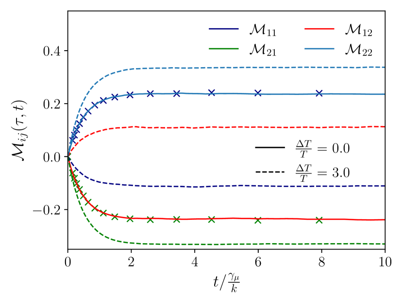
Figure 3: The entries of the MBR matrix for two coupled particles as in Eq. (55) with $\frac{\gamma_{1}}{\gamma_{2}}=1$ int the limit $\tau\to 0$ obtained from Langevin dynamics simulations. If both temperatures are the same the MBR matrix is symmetric with identical diagonal elements, shown by using crosses instead of the corresponding lines. If temperatures differ the symmetry is broken and the coordinates can be distinguished. The diagonal entries correspond to the one dimensional MBRs of the individual particles $x_{1}$ and $x_{2}$.

VII Density Mean Back Relaxation marks broken detailed balance in confinement and bulk

Recall from section III that MBR in a confined system marks broken detailed balance [23]. Such statement cannot be made in bulk [23], see section IV, due to absence of a well defined mean particle position $\langle x\rangle$ in that case. This issue can be overcome by introducing an observable that shows a well defined mean in bulk. We propose here to use the microscopic density in Fourier space [32] (for simplicity restricting to a one dimensional wave vector $q$)

$$\rho_{q}(t)=\sum_{j=1}^{N}e^{iqx_{j}(t)}.$$ (70)

Here, $j$ runs over the different particles of an $N$ particle system, or other coordinates. We continue under the assumption that the mean $\langle\rho_{q}\rangle$ is unique and well defined. Note that, e.g., for a single component fluid, $\langle\rho_{q}\rangle$ is the spatial Fourier transform of mean particle density, which is finite for typical particle interactions [32]. More specific, for homogeneous systems, the mean density is constant in space, and $\langle\rho_{q}\rangle$ vanishes for any finite $q$ [32].

We thus introduce the density mean back relaxation dMBR,

$$\mathcal{M}^{\rho}(\tau,t,q)=\left\langle-\frac{\rho_{q}(t)-\rho_{q}(0)}{\rho_{q}(0)-\rho_{q}(-\tau)}\right\rangle.$$ (71)

dMBR additionally depends on the wave vector $q$ compared to MBR. A global displacement $x_{i}+a$ yields a factor $\rho_{q}(t)\to e^{iqa}\rho_{q}(t)$, which cancels in Eq. (71). dMBR does thus not depend on the choice of coordinate origin. Most important, with detailed balance, we can thus state

$$\lim_{t\to\infty}\mathcal{M}^{\rho}(\tau,t,q)\overset{d.b.}{=}\frac{1}{2},$$ (72)

so that dMBR marks detailed balance. Furthermore, the sum of long time values of dMBR for normal and reversed trajectories adds up to unity, analogously to Eq. (14),

$$\lim_{t\to\infty}\mathcal{M}^{\rho}(\tau,t,q)+\lim_{t\to\infty}\mathcal{M}^{\rho}_{r}(\tau,t,q)=1.$$ (73)

To demonstrate these properties, we revisit the two coupled particles of Eq. (55), see Fig. 4. Indeed, for $T_{1}=T_{2}$, dMBR approaches $\frac{1}{2}$, while it deviates from $\frac{1}{2}$ for $T_{1}\not=T_{2}$, with Eq. (73) fulfilled. As expected, the deviation from $\frac{1}{2}$ depends on $q$, and we interpret that this dependence on $q$ allows to find the length scale of pronounced violation of detailed balance.

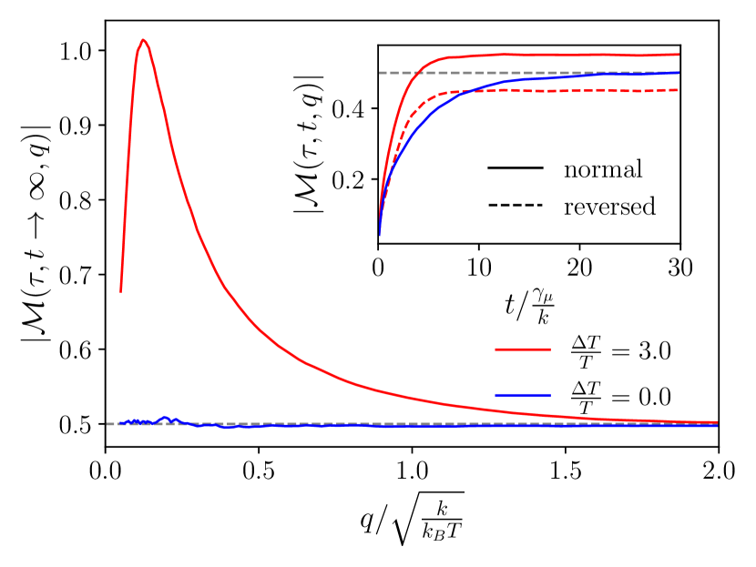
Figure 4: Density MBR, Eq. (71), for two coupled particles, see Eq. (55), with $\tau=0.1\frac{\gamma_{\mu}}{k}$ and $\frac{\gamma_{1}}{\gamma_{2}}=1$. Main plot shows the long time limit as a function of $q$, displaying the value of $\frac{1}{2}$ for equal temperatures, and a deviation for different temperatures. The deviation from $\frac{1}{2}$ is maximal for $q_{\text{max}}\approx 0.12\sqrt{\frac{k}{k_{B}T}}$ for this set of parameters. Inset shows the behavior for $q=0.8$ as a function of time, where we note that Eq. (73) is fulfilled.

VIII Discussion

In confined systems, the mean back relaxation MBR marks breakage of detailed balance [23]. We exemplify this for the case of a trapped active Brownian particle. In bulk, such statement cannot be made due to absence of a mean particle position. While there is no strict proof, for our bulk examples of overdamped cases, MBR in equilibrium takes values between zero and $\frac{1}{2}$ and is monotonic, while it can be negative for non-equilibrium cases. Using a path integral approach we find a general solution for the MBR in terms of multipoint density correlations. Evaluating this for Gaussian systems yields a relation between mean squared displacement (MSD) and MBR, from which additional properties of MBR in Gaussian equilibrium can be inferred. We finally proposed to use bound observables, such as the Fourier transform of microscopic density. Defining a density MBR, dMBR, enjoys, even in bulk, all properties of MBR in confinement: It marks breakage of detailed balance, and sums up to unity from normal and reversed paths.

Open questions concern the validity of the MBR-MSD formula beyond Gaussian systems. It also remains open whether monotonicity and positivity of MBR in equilibrium (bulk) can be proven more generally. For dMBR, more examples need to be studied, by testing it in many-body systems [40, 41].

Appendix A Calculation of MBR of Two Coupled Particles

The Langevin equations of the two linearly coupled particles, discussed in section VI.3, are give by

$$\dot{x}_{1} =-\frac{k}{\gamma_{1}}(x_{1}-x_{2})+f_{1}$$ (74a)

$$\dot{x}_{2} =-\frac{k}{\gamma_{2}}(x_{2}-x_{1})+f_{2}$$ (74b)

with coupling constant $k$, friction constants $\gamma_{i}$ and white noise random forces $\left\langle f_{i}(t)f_{j}(t^{\prime}\right\rangle=\frac{2k_{B}T_{i}}{\gamma_{i}}\delta_{ij}\delta(t-t^{\prime})$. To calculate the mean back relaxation (MBR) we calculate the mean squared displacement (MSD) $\Delta x^{2}(t)=\left\langle(x(t)-x(0))^{2}\right\rangle$ and apply result Eq. (47). Firstly we transform the Langevin equations by introducing the relative coordinate $x_{r}=x_{1}-x_{2}$ and the center coordinate $x_{s}=\frac{\gamma_{1}x_{1}+\gamma_{2}x_{2}}{\gamma_{1}+\gamma_{2}}$

$$\dot{x}_{r} =-k\left(\frac{1}{\gamma_{1}}+\frac{1}{\gamma_{2}}\right)x_{r}+f_{r}$$ (75a)

$$\dot{x}_{s} =f_{s}$$ (75b)

with $f_{r}=f_{1}-f_{2}$ and $f_{s}=\frac{\gamma_{1}f_{1}+\gamma_{2}f_{2}}{\gamma_{1}+\gamma_{2}}$. However, the random forces $f_{r}$ and $f_{s}$ are not necessarily uncorrelated and fullfill the following relations

$$\left\langle\xi_{r}(t)\xi_{r}(t^{\prime})\right\rangle =2k_{B}\left[\frac{T_{1}}{\gamma_{1}}+\frac{T_{2}}{\gamma_{2}}\right]\delta(t-t^{\prime})$$ (76a)

$$\left\langle\xi_{s}(t)\xi_{s}(t^{\prime})\right\rangle =2k_{B}\frac{T_{1}\gamma_{1}+T_{2}\gamma_{2}}{(\gamma_{1}+\gamma_{2})^{2}}\delta(t-t^{\prime})$$ (76b)

$$\left\langle\xi_{r}(t)\xi_{s}(t^{\prime})\right\rangle =2k_{B}\frac{T_{1}-T_{2}}{\gamma_{1}+\gamma_{2}}\delta(t-t^{\prime})$$ (76c)

In equilibrium $T_{1}=T_{2}$ the random forces $\left\langle f_{r}(t)f_{s}(t^{\prime})\right\rangle=0$ are uncorrelated, therefore, $x_{r}$ and $x_{s}$ are independent in equilibrium. By expressing the tracer coordinate as $x_{1}=x_{s}+\frac{\gamma_{2}}{\gamma_{1}+\gamma_{2}}x_{r}$ the means square displacement is given by

$$\Delta x_{1}^{2}(t) =\left<\left(x_{s}(t)+\frac{\gamma_{2}}{\gamma_{1}+\gamma_{2}}x_{r}(t)\right.\right.$$ (77)

$$\left.\left.\leavevmode\nobreak\ \leavevmode\nobreak\ \leavevmode\nobreak\ \leavevmode\nobreak\ \leavevmode\nobreak\ -x_{s}(0)-\frac{\gamma_{2}}{\gamma_{1}+\gamma_{2}}x_{r}(0)\right)^{2}\right>$$

$$=\Delta x_{s}^{2}(t)+\frac{\gamma_{2}^{2}}{(\gamma_{1}+\gamma_{2})^{2}}\Delta x_{r}^{2}(t)$$ (78)

$$=\frac{2k_{B}T}{\gamma_{1}+\gamma_{2}}t+\frac{2k_{B}T\gamma_{2}^{2}}{k(\gamma_{1}+\gamma_{2})^{2}}\left(1-e^{-\frac{k}{\gamma_{\mu}}t}\right)$$ (79)

with $\gamma_{\mu}=\frac{1}{\gamma_{1}}+\frac{1}{\gamma_{2}}$ and using that $x_{s}$ reassembles a freely diffusing particle and $x_{r}$ a particle in a harmonic potential. The MBR is then determined by Eq. (47)

$$\mathcal{M}_{\tau}(t)=\frac{\gamma_{2}^{2}}{2}\frac{\left(1-e^{-\frac{k}{\gamma_{\mu}}t}\right)\left(1-e^{-\frac{k}{\gamma_{\mu}}\tau}\right)}{k(\gamma_{1}+\gamma_{2})\tau+\gamma_{2}^{2}\left(1-e^{-\frac{k}{\gamma_{\mu}}\tau}\right)}.$$ (80)

In non-equilibrium $T_{1}\neq T_{2}$ we have to take the correlations of $x_{s}$ and $x_{r}$ into account. The overall MSD is therefore given by

$$\begin{split}\left\langle(x_{1}(t)-x_{1}(0))^{2}\right\rangle=\Delta x_{s}^{2}(t)+\frac{\gamma_{2}^{2}}{(\gamma_{1}+\gamma_{2})^{2}}\Delta x_{r}^{2}(t)\\ +2\frac{\gamma_{2}}{\gamma_{1}+\gamma_{2}}\left\langle(x_{s}(t)-x_{s}(0))(x_{r}(t)-x_{r}(0))\right\rangle.\end{split}$$ (81)

The MSD of center coordinated $x_{s}$ and $x_{r}$ get small corrections rising from the temperature difference $\Delta T=T_{2}-T_{1},T_{1}=T$ and are given by

$$\Delta x_{s}^{2}(t) =\frac{2k_{B}T}{\gamma_{1}+\gamma_{2}}t+\frac{2k_{B}\Delta T\gamma_{2}}{(\gamma_{1}+\gamma_{2})^{2}}t$$ (82)

$$\Delta x_{r}^{2}(t) =\frac{2k_{B}}{k}\left(T+\frac{\gamma_{1}}{\gamma_{1}+\gamma_{2}}\Delta T\right)\left(1-e^{-\frac{k}{\gamma_{\mu}}t}\right).$$ (83)

The cross correlations are given by the formal solutions

$$x_{s}(t) =x_{a}+\int_{0}^{t}\text{d}s\leavevmode\nobreak\ \xi_{s}(s)$$ (84)

$$x_{r}(t) =x_{b}+\int_{0}^{t}\text{d}s\leavevmode\nobreak\ e^{-\frac{k}{\gamma_{\mu}}(t-s)}\xi_{r}(s)$$ (85)

with some initial conditions $x_{a}$ and $x_{b}$. The cross correlation is then given by

$$\left\langle x_{r}(t)x_{s}(t^{\prime})\right\rangle=e^{-\frac{k}{\gamma_{\mu}}t}\left(x_{a}x_{b}-\frac{2k_{B}\Delta T}{\gamma_{1}+\gamma_{2}}\frac{\gamma_{\mu}}{k}\left(e^{\frac{k}{\gamma_{\mu}}\min(t,t^{\prime})}-1\right)\right)$$ (86)

Inserting all terms into Eq. (81) gives the final result for the MSD

$$\begin{split}\Delta x_{1}^{2}(t)&=\frac{2k_{B}}{\gamma_{1}+\gamma_{2}}\left(T+\frac{\gamma_{2}}{\gamma_{1}+\gamma_{2}}\Delta T\right)t\\ &+\frac{2k_{B}}{k}\frac{\gamma_{2}^{2}}{(\gamma_{1}+\gamma_{2})^{2}}\left(T-\frac{\gamma_{1}}{\gamma_{1}+\gamma_{2}}\Delta T\right)\left(1-e^{-\frac{k}{\gamma_{\mu}}t}\right)\end{split}$$ (87)

and via Eq. (47) the final result for the MBR

$$\mathcal{M}(\tau,t)=\frac{1}{2}\frac{\gamma_{2}^{2}\left(T-\frac{\gamma_{1}}{\gamma_{1}+\gamma_{2}}\Delta T\right)\left(1-e^{-\frac{k}{\gamma_{\mu}}t}\right)\left(1-e^{-\frac{k}{\gamma_{\mu}}\tau}\right)}{k(\gamma_{1}+\gamma_{2})\left(T+\frac{\gamma_{2}}{\gamma_{1}+\gamma_{2}}\Delta T\right)\tau+\gamma_{2}^{2}\left(T-\frac{\gamma_{1}}{\gamma_{1}+\gamma_{2}}\Delta T\right)\left(1-e^{-\frac{k}{\gamma_{\mu}}\tau}\right)}.$$ (88)

By expressing time in multiples of $\frac{\gamma_{\mu}}{k}$, the characteristic time scale of the system, the MBR takes the form

$$\mathcal{M}(\tau,t)=\frac{1}{2}\frac{\left(1-\frac{\gamma_{1}/\gamma_{2}}{1+\gamma_{1}/\gamma_{2}}\frac{\Delta T}{T}\right)\left(1-e^{-t}\right)\left(1-e^{-\tau}\right)}{\frac{\gamma_{1}}{\gamma_{2}}\left(1+\frac{1}{1+\gamma_{1}/\gamma_{2}}\frac{\Delta T}{T}\right)\tau+\left(1-\frac{\gamma_{1}/\gamma_{2}}{1+\gamma_{1}/\gamma_{2}}\frac{\Delta T}{T}\right)\left(1-e^{-\tau}\right)}$$ (89)

and only depends on the dimensionless quantities $\frac{\gamma_{1}}{\gamma_{2}}$ and $\frac{\Delta T}{T}$. The solution for the diffusing potential model, discussed in section IV is obtained by taking the limit $T_{2},\gamma_{2}\to\infty$, by keeping the ratio $\frac{k_{B}T_{2}}{\gamma_{2}}=D_{q}$ fixed. With $\frac{k_{B}T_{1}}{\gamma_{1}}=D$ the solution of the MBR is given by

$$\mathcal{M}(\tau,t)=\frac{D-D_{q}}{\frac{k}{\gamma_{1}}}\frac{\left(1-e^{-\frac{k}{\gamma_{1}}t}\right)\left(1-e^{-\frac{k}{\gamma_{1}}\tau}\right)}{2D_{q}\tau+\frac{2(D-D_{q})}{\frac{k}{\gamma_{1}}}\left(1-e^{-\frac{k}{\gamma_{1}}\tau}\right)}$$ (90)

with the limiting case

$$\lim_{t\to\infty}\lim_{\tau\to 0}\mathcal{M}(\tau,t)=\frac{1}{2}\left(1-\frac{D_{q}}{D}\right).$$ (91)

References

• [1] T. M. Squires and T. G. Mason, “Fluid Mechanics of Microrheology,” Annual Review of Fluid Mechanics, vol. 42, p. 413–438, Jan. 2010.
• [2] D. Krapf, E. Marinari, R. Metzler, G. Oshanin, X. Xu, and A. Squarcini, “Power spectral density of a single Brownian trajectory: what one can and cannot learn from it,” New Journal of Physics, vol. 20, p. 023029, Feb. 2018.
• [3] P. Martin, A. J. Hudspeth, and F. Jülicher, “Comparison of a hair bundle’s spontaneous oscillations with its response to mechanical stimulation reveals the underlying active process,” Proceedings of the National Academy of Sciences, vol. 98, p. 14380–14385, Dec. 2001.
• [4] W. W. Ahmed, É. Fodor, M. Almonacid, M. Bussonnier, M.-H. Verlhac, N. Gov, P. Visco, F. v. Wijland, and T. Betz, “Active Mechanics Reveal Molecular-Scale Force Kinetics in Living Oocytes,” Biophysical Journal, vol. 114, no. 7, p. 1667–1679, 2018.
• [5] K. Hubicka and J. Janczura, “Time-dependent classification of protein diffusion types: A statistical detection of mean-squared-displacement exponent transitions,” Physical Review E, vol. 101, p. 022107, Feb. 2020.
• [6] R. Kubo, “The fluctuation-dissipation theorem,” Reports on Progress in Physics, vol. 29, p. 255, Jan. 1966.
• [7] G. S. Agarwal, “Fluctuation-dissipation theorems for systems in non-thermal equilibrium and applications,” Zeitschrift für Physik A Hadrons and nuclei, vol. 252, p. 25–38, Feb. 1972.
• [8] T. Harada and S.-i. Sasa, “Equality Connecting Energy Dissipation with a Violation of the Fluctuation-Response Relation,” Physical Review Letters, vol. 95, p. 130602, Sept. 2005.
• [9] T. Speck and U. Seifert, “Restoring a fluctuation-dissipation theorem in a nonequilibrium steady state,” Europhysics Letters (EPL), vol. 74, p. 391–396, May 2006.
• [10] M. Baiesi, C. Maes, and B. Wynants, “Fluctuations and response of nonequilibrium states,” Physical Review Letters, vol. 103, p. 010602, July 2009. arXiv:0902.3955 [cond-mat].
• [11] M. Baiesi and C. Maes, “An update on the nonequilibrium linear response,” New Journal of Physics, vol. 15, p. 013004, Jan. 2013.
• [12] R. K. P. Zia and B. Schmittmann, “Probability currents as principal characteristics in the statistical mechanics of non-equilibrium steady states,” Journal of Statistical Mechanics: Theory and Experiment, vol. 2007, p. P07012–P07012, July 2007.
• [13] U. Seifert, “Stochastic thermodynamics, fluctuation theorems and molecular machines,” Reports on Progress in Physics, vol. 75, p. 126001, Nov. 2012. Publisher: IOP Publishing.
• [14] A. C. Barato and U. Seifert, “Thermodynamic Uncertainty Relation for Biomolecular Processes,” Physical Review Letters, vol. 114, p. 158101, Apr. 2015.
• [15] J. M. Horowitz and T. R. Gingrich, “Thermodynamic uncertainty relations constrain non-equilibrium fluctuations,” Nature Physics, vol. 16, p. 15–20, Jan. 2020.
• [16] C. Dieball and A. Godec, “Direct Route to Thermodynamic Uncertainty Relations and Their Saturation,” Physical Review Letters, vol. 130, p. 087101, Feb. 2023.
• [17] A. Ghanta, J. C. Neu, and S. Teitsworth, “Fluctuation loops in noise-driven linear dynamical systems,” Physical Review E, vol. 95, p. 032128, Mar. 2017.
• [18] S. Thapa, D. Zaretzky, R. Vatash, G. Gradziuk, C. Broedersz, Y. Shokef, and Y. Roichman, “Nonequilibrium probability currents in optically-driven colloidal suspensions,” 2023.
• [19] G. Knotz, T. M. Muenker, T. Betz, and M. Krüger, “Entropy bound for time reversal markers,” Feb. 2023. arXiv:2302.07709 [cond-mat].
• [20] É’. Roldá’n, I. Neri, M. Dörpinghaus, H. Meyr, and F. Jülicher, “Decision Making in the Arrow of Time,” Physical Review Letters, vol. 115, p. 250602, Dec. 2015.
• [21] J. Berner, B. Müller, J. R. Gomez-Solano, M. Krüger, and C. Bechinger, “Oscillating modes of driven colloids in overdamped systems,” Nature Communications, vol. 9, no. 1, p. 999, 2018.
• [22] F. Mori, S. N. Majumdar, and G. Schehr, “Time to reach the maximum for a stationary stochastic process,” Physical Review E, vol. 106, p. 054110, Nov. 2022.
• [23] T. M. Muenker, G. Knotz, M. Krüger, and T. Betz, “Onsager regression characterizes living systems in passive measurements,” bioRxiv, 2022. bioRxiv:2022.05.15.491928.
• [24] P. Ronceray, “Two steps forward – and one step back?– Measuring fluctuation-dissipation breakdown from fluctuations only,” Journal Club for Condensed Matter Physics, July 2023.
• [25] C. Maes and K. Netočný, “Time-reversal and entropy,” Journal of Statistical Physics, vol. 110, no. 1, p. 269–310, 2003.
• [26] U. Seifert, “Entropy Production along a Stochastic Trajectory and an Integral Fluctuation Theorem,” Physical Review Letters, vol. 95, p. 040602, July 2005.
• [27] C. Bechinger, R. Di Leonardo, H. Löwen, C. Reichhardt, G. Volpe, and G. Volpe, “Active Particles in Complex and Crowded Environments,” Reviews of Modern Physics, vol. 88, p. 045006, Nov. 2016.
• [28] O. Dauchot and V. Démery, “Dynamics of a Self-Propelled Particle in a Harmonic Trap,” Physical Review Letters, vol. 122, p. 068002, Feb. 2019.
• [29] A. Altland and B. D. Simons, Condensed Matter Field Theory. Cambridge University Press, 2 ed., 2010.
• [30] J. A. Hertz, Y. Roudi, and P. Sollich, “Path integral methods for the dynamics of stochastic and disordered systems,” Journal of Physics A: Mathematical and Theoretical, vol. 50, p. 033001, Dec. 2016. Publisher: IOP Publishing.
• [31] J. K. G. Dhont, “Studies in Interface Science,” in An Introduction to Dynamics of Colloids, vol. 2 of Studies in Interface Science, Elsevier, 1996. ISSN: 1383-7303.
• [32] J. Hansen and I. McDonald, Theory of Simple Liquids: with Applications to Soft Matter. Elsevier Science, 2013.
• [33] M. Helias and D. Dahmen, Statistical Field Theory for Neural Networks. Springer International Publishing, 2020.
• [34] T. J. Doerries, S. A. M. Loos, and S. H. L. Klapp, “Correlation functions of non-Markovian systems out of equilibrium: analytical expressions beyond single-exponential memory,” Journal of Statistical Mechanics: Theory and Experiment, vol. 2021, p. 033202, Mar. 2021.
• [35] M. Khan and T. G. Mason, “Trajectories of probe spheres in generalized linear viscoelastic complex fluids,” Soft Matter, vol. 10, p. 9073–9081, Sept. 2014.
• [36] F. Ginot, J. Caspers, L. F. Reinalter, K. Krishna Kumar, M. Krüger, and C. Bechinger, “Recoil experiments determine the eigenmodes of viscoelastic fluids,” New Journal of Physics, vol. 24, p. 123013, Dec. 2022.
• [37] J. Caspers, N. Ditz, K. Krishna Kumar, F. Ginot, C. Bechinger, M. Fuchs, and M. Krüger, “How are mobility and friction related in viscoelastic fluids?,” The Journal of Chemical Physics, vol. 158, p. 024901, Jan. 2023.
• [38] G. Weiss, “Time-Reversibility of Linear Stochastic Processes,” Journal of Applied Probability, vol. 12, no. 4, p. 831–836, 1975. Publisher: Applied Probability Trust.
• [39] H. Risken, The Fokker-Planck equation: methods of solution and applications. No. v. 18 in Springer series in synergetics, New York: Springer-Verlag, 2nd ed ed., 1996.
• [40] J. S. Hub, T. Salditt, M. C. Rheinstädter, and B. L. De Groot, “Short-Range Order and Collective Dynamics of DMPC Bilayers: A Comparison between Molecular Dynamics Simulations, X-Ray, and Neutron Scattering Experiments,” Biophysical Journal, vol. 93, p. 3156–3168, Nov. 2007.
• [41] N. Grimm, A. Zippelius, and M. Fuchs, “Simple fluid with broken time-reversal invariance,” Physical Review E, vol. 106, p. 034604, Sept. 2022.