Electroweak Strings in the Standard Model

Abstract

We argue that the existence of the electroweak monopole predicts the existence of the electroweak string in the standard model made of monopole-antimonopole pair separated infinitely apart, which carry the quantized magnetic flux $4\pi n/e$. We show how to construct such quantized magnetic flux string solution. Our result strongly indicates that genuine fundamental electromagnetic string could exist in nature which could actually be detected. We discuss the physical implications of our result in cosmology.

I Introduction

With the recent discovery of Higgs particle at LHC, it has been widely regarded that the standard model has passed the “final” test [1]. This has urged people to go “beyond” the standard model. But we emphasize that this view might be premature, because it has yet to pass another important test, the topological test. By now it is well known that the standard model must have the electroweak (Cho-Maison) monopole as the electroweak generalization of Dirac monopole [2, 3]. And this is within, not beyond, the standard model. This means that the true final test of the standard model should come from the discovery of the topological objects of the model, in particular the electroweak monopole.

After Dirac predicted the existence of the monopole, the monopole has become an obsession [4, 5]. But the Dirac monopole, in the course of the electroweak unification of the weak and electromagnetic interactions, changes to the electroweak monopole [2, 3]. So, the monopole which should exist in the real world is not the Dirac monopole but this one. This has triggered new studies on the electroweak monopole [6, 7, 8, 9, 10, 11, 12, 13, 14, 15]. Moreover, if detected it will become the first magnetically charged topological elementary particle in the history of physics. For this reason MoEDAL and ATLAS at LHC, IceCube at the south pole as well as other detectors are actively searching for such monopole [16, 17, 18].

If the standard model has the monopole, it must also have another important topological object, the quantized magnetic vortex. This is because the electroweak monopole predicts the existence of the electroweak string made of the monopole-antimonopole pair which carries the quantized magnetic flux $4\pi n/e$. This is not surprising. Since the standard model includes the unbroken electromagnetic U(1) interaction it is natural to expect that it has the magnetic vortex. The purpose of this paper is to demonstrate the existence of the electromagnetic string carrying the quantized magnetic flux in the standard model, and to discuss the physical implications of the string.

Of course, it has been well known that the standard model has the string solution known as the Nambu string, W string, and Z-string [19, 20, 21]. But here we are talking about a new type of string, the electromagnetic string which carries quantized magnetic flux.

The existence of the electromagnetic string in the standard model should have deep implications in physics. Clearly it could be interpreted as a fundamental topological string in nature, so that it has an important theoretical meaning. Moreover, it could play an important role in cosmology, in particular in the early universe in the formation of large scale structure of the universe [22].

The paper is organized as follows. In Section II we review the Abelian decomposition of the standard model for to clarify the topological structure of the model. In Section III we review the electroweak monopole for later use. In Section IV we discuss the possible string ansatz and string equation of motion in the standard model, in particular the magnetic vortex solution made of the infinitely separated monopole-antimonopole pair. In Section V we discuss the electroweak vortex solution carrying quantized magnetic flux in the standard model. In Section VI we compare this string solution with the known Z-string solution. Finally in the last section we discuss the physical implications of our results.

II Abelian Decomposition of the Standard Model: A Review

Before we discuss the electroweak string it is important for us to understand the structure of the standard model. For this we start from the gauge independent Abelian decomposition of the electroweak theory. Consider the (bosonic sector of) Weinberg-Salam model,

$${\cal L}=-|{\cal D}_{\mu}\phi|^{2}-\frac{\lambda}{2}\big{(}|\phi|^{2}-\frac{\mu^{2}}{\lambda}\big{)}^{2}-\frac{1}{4}{\vec{F}}_{\mu\nu}^{2}-\frac{1}{4}G_{\mu\nu}^{2},$$

$${\cal D}_{\mu}\phi=\big{(}\partial_{\mu}-i\frac{g}{2}{\vec{\sigma}}\cdot{\vec{A}}_{\mu}-i\frac{g^{\prime}}{2}B_{\mu}\big{)}\phi$$

$$=D_{\mu}\phi-i\frac{g^{\prime}}{2}B_{\mu}\phi,$$ (1)

where $\phi$ is the Higgs doublet, ${\vec{A}}_{\mu}$, ${\vec{F}}_{\mu\nu}$ and $B_{\mu}$, $G_{\mu\nu}$ are the gauge fields of $SU(2)$ and hypercharge $U(1)_{Y}$, and $D_{\mu}$ is the covariant derivative of $SU(2)$. With

$$\phi=\dfrac{1}{\sqrt{2}}\rho~{}\xi,~{}~{}~{}(\xi^{\dagger}\xi=1),$$ (2)

we have

$${\cal L}=-\frac{1}{2}(\partial_{\mu}\rho)^{2}-\frac{\rho^{2}}{2}|{\cal D}_{\mu}\xi|^{2}-\frac{\lambda}{8}\big{(}\rho^{2}-\rho_{0}^{2}\big{)}^{2}$$

$$-\frac{1}{4}{\vec{F}}_{\mu\nu}^{2}-\frac{1}{4}G_{\mu\nu}^{2},$$ (3)

where $\rho_{0}=\sqrt{2\mu^{2}/\lambda}$ is the vacuum value of the Higgs field. Notice that the $U(1)_{Y}$ coupling of $\xi$ makes the theory a gauge theory of $CP^{1}$ field [2].

Let $(\hat{n}_{1},\hat{n}_{2},\hat{n}_{3}=\hat{n})$ be an arbitrary right-handed orthonormal basis of $SU(2)$. Identifying $\hat{n}$ to be the Abelian direction at each space-time point, we have the Abelian decomposition of the $SU(2)$ gauge field to the restricted part ${\hat{A}}_{\mu}$ and the valence part ${\vec{W}}_{\mu}$ [23, 24],

$${\vec{A}}_{\mu}={\hat{A}}_{\mu}+{\vec{W}}_{\mu},$$

$${\hat{A}}_{\mu}={\tilde{A}}_{\mu}+{\tilde{C}}_{\mu},~{}~{}~{}{\vec{W}}_{\mu}=W^{1}_{\mu}~{}\hat{n}_{1}+W^{2}_{\mu}~{}\hat{n}_{2},$$

$${\tilde{A}}_{\mu}=A_{\mu}\hat{n}~{}~{}(A_{\mu}=\hat{n}\cdot{\vec{A}}_{\mu}),~{}~{}~{}{\tilde{C}}_{\mu}=-\frac{1}{g}\hat{n}\times\partial_{\mu}\hat{n},$$

$${\vec{F}}_{\mu\nu}={\hat{F}}_{\mu\nu}+{\hat{D}}_{\mu}{\vec{W}}_{\nu}-{\hat{D}}_{\nu}{\vec{W}}_{\mu}+g{\vec{W}}_{\mu}\times{\vec{W}}_{\nu},$$

$${\hat{D}}_{\mu}=\partial_{\mu}+g{\hat{A}}_{\mu}\times.$$ (4)

It has the following properties. First, ${\hat{A}}_{\mu}$ is made of two potentials, the non-topological ${\tilde{A}}_{\mu}$ and topological ${\tilde{C}}_{\mu}$. Second, it has the full $SU(2)$ gauge degrees of freedom, in spite of the fact that it is restricted. Third, ${\vec{W}}_{\mu}$ transforms gauge covariantly. Most importantly, the decomposition is gauge independent. Once the Abelian direction is chosen it follows automatically, regardless of the choice of gauge.

The restricted field strength ${\hat{F}}_{\mu\nu}$ inherits the dual structure of ${\hat{A}}_{\mu}$, which can also be described by two potentials $A_{\mu}$ and $C_{\mu}$,

$${\hat{F}}_{\mu\nu}=\partial_{\mu}{\hat{A}}_{\nu}-\partial_{\nu}{\hat{A}}_{\mu}+g{\hat{A}}_{\mu}\times{\hat{A}}_{\nu}=F_{\mu\nu}^{\prime}\hat{n},$$

$$F^{\prime}_{\mu\nu}=F_{\mu\nu}+H_{\mu\nu}=\partial_{\mu}A^{\prime}_{\nu}-\partial_{\nu}A^{\prime}_{\mu},$$

$$F_{\mu\nu}=\partial_{\mu}A_{\nu}-\partial_{\nu}A_{\mu},$$

$$H_{\mu\nu}=-\frac{1}{g}\hat{n}\cdot(\partial_{\mu}\hat{n}\times\partial_{\nu}\hat{n})=\partial_{\mu}C_{\nu}-\partial_{\nu}C_{\mu},$$

$$\hat{n}=-\xi^{\dagger}{\vec{\sigma}}\xi,$$

$$C_{\mu}\simeq-\frac{1}{g}\hat{n}_{1}\cdot\partial_{\mu}\hat{n}_{2}\simeq-\frac{2i}{g}\xi^{\dagger}\partial_{\mu}\xi,$$

$$A_{\mu}^{\prime}=A_{\mu}+C_{\mu}.$$ (5)

Although ${\hat{F}}_{\mu\nu}$ has only the Abelian component, it describes the non-trivial U(1) gauge theory, because it has not only the Maxwellian $A_{\mu}$ but also the Diracian $C_{\mu}$ which describes the monopole potential [23, 24]. This justifies us to call $A_{\mu}$ and $C_{\mu}$ the non-topological electric and topological magnetic potential.

With the Abelian decomposition we can express (1) in terms of physical fields in an Abelian form gauge independently. To do this we first define the electromagnetic and Z boson fields $A_{\mu}^{\rm(em)}$ and $Z_{\mu}$ with the Weinberg angle by

$$\left(\begin{array}[]{cc}A_{\mu}^{\rm(em)}\\ Z_{\mu}\end{array}\right)=\frac{1}{\sqrt{g^{2}+g^{\prime 2}}}\left(\begin{array}[]{cc}g&g^{\prime}\\ -g^{\prime}&g\end{array}\right)\left(\begin{array}[]{cc}B_{\mu}\\ A^{\prime}_{\mu}\end{array}\right)$$ (12)

$$=\left(\begin{array}[]{cc}\cos\theta_{\rm w}&\sin\theta_{\rm w}\\ -\sin\theta_{\rm w}&\cos\theta_{\rm w}\end{array}\right)\left(\begin{array}[]{cc}B_{\mu}\\ A_{\mu}^{\prime}\end{array}\right).$$ (17)

Now, with the identity

$$D_{\mu}\xi=-i\frac{g}{2}\big{[}(A^{\prime}_{\mu}\hat{n}+{\vec{W}}_{\mu})\cdot{\vec{\sigma}}\big{]}~{}\xi,$$

$$|D_{\mu}\xi|^{2}=\frac{g^{2}}{4}({A^{\prime}}_{\mu}^{2}+{\vec{W}}_{\mu}^{2}),$$

$$|{\cal D}_{\mu}\xi|^{2}=\frac{g^{2}+g^{\prime 2}}{8}Z_{\mu}^{2}+\frac{g^{2}}{4}{\vec{W}}_{\mu}^{2},$$ (18)

we can “abelianize” (1) to

$${\cal L}=-\frac{1}{2}(\partial_{\mu}\rho)^{2}-\frac{\lambda}{8}\big{(}\rho^{2}-\rho_{0}^{2}\big{)}^{2}-\frac{1}{4}{F_{\mu\nu}^{\rm(em)}}^{2}$$

$$-\frac{1}{2}\big{|}(D_{\mu}^{\rm(em)}+ie\frac{g}{g^{\prime}}Z_{\mu})W_{\nu}-(D_{\nu}^{\rm(em)}+ie\frac{g}{g^{\prime}}Z_{\nu})W_{\mu}\big{|}^{2}$$

$$-\frac{1}{4}Z_{\mu\nu}^{2}-\frac{\rho^{2}}{4}\big{(}g^{2}W_{\mu}^{*}W_{\mu}+\frac{g^{2}+g^{\prime 2}}{2}Z_{\mu}^{2}\big{)}$$

$$+ie(F_{\mu\nu}^{\rm(em)}+\frac{g}{g^{\prime}}Z_{\mu\nu})W_{\mu}^{*}W_{\nu}+\frac{g^{2}}{4}(W_{\mu}^{*}W_{\nu}-W_{\nu}^{*}W_{\mu})^{2},$$

$$D_{\mu}^{\rm(em)}=\partial_{\mu}+ieA_{\mu}^{\rm(em)},~{}~{}~{}W_{\mu}=\frac{1}{\sqrt{2}}(W^{1}_{\mu}+iW^{2}_{\mu}),$$

$$e=\frac{gg^{\prime}}{\sqrt{g^{2}+g^{\prime 2}}}=g\sin\theta_{\rm w}=g^{\prime}\cos\theta_{\rm w}.$$ (19)

This is the gauge independent Abelianization of the standard model.

From (19) we obtain the following equations of motion

$$\partial^{2}\rho-\big{(}\frac{g^{2}}{2}W_{\mu}^{*}W_{\mu}+\frac{g^{2}+g^{\prime 2}}{4}Z_{\mu}^{2}\big{)}~{}\rho=\frac{\lambda}{2}\big{(}\rho^{2}-\rho_{0}^{2}\big{)}~{}\rho,$$

$$\partial_{\mu}\Big{[}F_{\mu\nu}^{\rm(em)}-ie(W_{\mu}^{*}W_{\nu}-W_{\nu}^{*}W_{\mu})\Big{]}=ie\Big{[}W_{\mu}^{*}(D_{\mu}^{\rm(em)}W_{\nu}$$

$$-D_{\nu}^{\rm(em)}W_{\mu})-(D_{\mu}^{\rm(em)}W_{\nu}-D_{\nu}^{\rm(em)}W_{\mu})^{*}W_{\mu}\Big{]}$$

$$+e^{2}\frac{g}{g^{\prime}}\Big{[}2W_{\mu}^{*}W_{\mu}Z_{\nu}-Z_{\mu}(W_{\mu}^{*}W_{\nu}+W_{\nu}^{*}W_{\mu})\Big{]},$$

$$\Big{(}D_{\mu}^{\rm(em)}+ie\frac{g}{g^{\prime}}Z_{\mu}\Big{)}\Big{[}D_{\mu}^{\rm(em)}W_{\nu}-D_{\nu}^{\rm(em)}W_{\mu}$$

$$+ie\frac{g}{g^{\prime}}(Z_{\mu}W_{\nu}-Z_{\nu}W_{\mu})\Big{]}=\frac{g^{2}}{4}\rho^{2}W_{\nu}$$

$$+ieW_{\mu}\big{(}F^{\rm(em)}_{\mu\nu}+\frac{g}{g^{\prime}}Z_{\mu\nu}\big{)}+g^{2}W_{\mu}(W_{\mu}^{*}W_{\nu}-W_{\nu}^{*}W_{\mu}),$$

$$\partial_{\mu}\Big{[}Z_{\mu\nu}-ie\frac{g}{g^{\prime}}(W_{\mu}^{*}W_{\nu}-W_{\mu}W_{\nu}^{*})\Big{]}-\frac{g^{2}+g^{\prime 2}}{4}\rho^{2}Z_{\nu}$$

$$=ie\frac{g}{g^{\prime}}\Big{[}W_{\mu}^{*}(D_{\mu}^{\rm(em)}W_{\nu}-D_{\nu}^{\rm(em)}W_{\mu})$$

$$-W_{\mu}(D_{\mu}^{\rm(em)}W_{\nu}-D_{\nu}^{\rm(em)}W_{\mu})\Big{]}$$

$$+e^{2}\frac{g^{2}}{g^{\prime 2}}\Big{[}2W_{\mu}^{*}W_{\mu}Z_{\nu}-Z_{\mu}(W_{\mu}^{*}W_{\nu}+W_{\nu}^{*}W_{\mu})\Big{]}.$$ (20)

This should be compared with the equations of motion obtained from (3),

$$\partial^{2}\rho=|{\cal D}_{\mu}\xi|^{2}\rho+\frac{\lambda}{2}\big{(}\rho^{2}-\rho_{0}^{2}\big{)}\rho,$$

$${\cal D}^{2}\xi=-2\dfrac{\partial_{\mu}\rho}{\rho}{\cal D}_{\mu}\xi+\big{[}\xi^{\dagger}{\cal D}^{2}\xi+2\dfrac{\partial_{\mu}\rho}{\rho}(\xi^{\dagger}{\cal D}_{\mu}\xi)\big{]}\xi,$$

$$D_{\mu}{\vec{F}}_{\mu\nu}=i\frac{g}{4}\rho^{2}\big{[}\xi^{\dagger}\vec{\tau}({\cal D}_{\nu}\xi)-({\cal D}_{\nu}\xi)^{\dagger}\vec{\tau}\xi\big{]},$$

$$\partial_{\mu}G_{\mu\nu}=i\frac{g^{\prime}}{4}\rho^{2}\big{[}\xi^{\dagger}({\cal D}_{\nu}\xi)-({\cal D}_{\nu}\xi)^{\dagger}\xi\big{]}.$$ (21)

The contrast is unmistakable.

This Abelianization teaches us an important lesson, the assertion that the Higgs mechanism comes from the spontaneous symmetry breaking, is a simple misunderstanding. To see this notice that (19) is mathematically identical to (1). This means that (19) still retains the full non-Abelian $SU(2)\times U(1)_{Y}$ gauge symmetry. In fact, the non-Abelian gauge symmetry is hidden in the fact that $A_{\mu}^{(em)}$ and $Z_{\mu}$ are defined in terms of $A^{\prime}_{\mu}$ made of two potentials $A_{\mu}$ and $C_{\mu}$.

Nevertheless, the W and Z bosons acquire mass when $\rho$ has the non-vanishing vacuum value in (19). This means that we have the Higgs mechanism (i.e., the mass generation) without any (spontaneous or not) symmetry breaking. In fact, in (19) we have no Higgs doublet which can break the $SU(2)\times U(1)_{Y}$ symmetry. This confirms that the Higgs mechanism has nothing to do with the spontaneous symmetry breaking.

The above exercise tells us that the standard model has another important topology, the $\pi_{1}(S^{1})$ string topology which implies the existence of a topological string, in particular the electromagnetic string. Actually the Abelian decomposition tells that the standard model has two $\pi_{1}(S^{1})$ topology, coming from the unbroken electromagnetic $U(1)$ and the spontaneously broken Z boson $U(1)$, which strongly implies the existence of two types of strings.

Indeed, in the absence of weak bosons (19) reduces to the non-trivial electrodynamics

$${\cal L}=-\frac{1}{4}{F_{\mu\nu}^{\rm(em)}}^{2},$$ (22)

which has the Dirac-type electroweak monopole of magnetic charge $4\pi/e$. This is because the electromagnetic $U(1)_{em}$ here is non-trivial which has the period $4\pi$ (not $2\pi$). This is evident from (17), which tells that $U(1)_{em}$ comes from the superposition of the $U(1)$ subgroup of $SU(2)$.

This strongly implies that it also admits the electromagnetic string made of the monopole-antimonopole pair carrying the magnetic flux $4\pi/e$. Moreover, in the absence of $A_{\mu}^{\rm(em)}$ and $W$-boson (19) reduces to the spontaneously broken $U(1)_{Z}$ gauge theory,

$${\cal L}=-\frac{1}{2}(\partial_{\mu}\rho)^{2}-\frac{\lambda}{8}(\rho^{2}-\rho_{0}^{2})^{2}-\frac{1}{4}Z_{\mu\nu}^{2}$$

$$-\dfrac{g^{2}+g^{\prime 2}}{8}\rho^{2}Z_{\mu}^{2},$$ (23)

which describes the Landau-Ginzburg Lagrangian of superconductivity which is well known to have the Abrokosov-Nielsen-Olesen (ANO) vortex solution [25]. In the following we show how to obtain such string solutions in the standard model.

III Electroweak Monopole: A Review

Before we discuss the string solution, we review the electroweak monopole, because the string is deeply related to the monopole-antimonopole pair. Start from the monopole ansatz in the spherical coordinates $(t,r,\theta,\varphi)$ [2, 3]

$$\phi=\frac{i}{\sqrt{2}}\rho(r)\left(\begin{array}[]{cc}\sin\dfrac{\theta}{2}~{}\exp(-i\varphi)\\ -\cos\dfrac{\theta}{2}\end{array}\right),$$ (26)

$${\vec{A}}_{\mu}=\frac{1}{g}A(r)\partial_{\mu}t~{}\hat{r}+\frac{1}{g}(f(r)-1)~{}\hat{r}\times\partial_{\mu}\hat{r},$$

$$B_{\mu}=\frac{1}{g^{\prime}}B(r)\partial_{\mu}t-\frac{1}{g^{\prime}}(1-\cos\theta)\partial_{\mu}\varphi.$$ (27)

In terms of physical fields the ansatz becomes

$$\rho=\rho(r),$$

$$W_{\mu}=\frac{i}{g}\frac{f}{\sqrt{2}}e^{i\varphi}(\partial_{\mu}\theta+i\sin\theta\partial_{\mu}\varphi),$$

$$A_{\mu}^{\rm(em)}=e\big{(}\frac{A}{g^{2}}+\frac{B}{g^{\prime 2}}\big{)}\partial_{\mu}t-\frac{1}{e}(1-\cos\theta)\partial_{\mu}\varphi,$$

$$Z_{\mu}=\frac{e}{gg^{\prime}}\big{(}A-B\big{)}\partial_{\mu}t.$$ (28)

This clearly shows that the ansatz is for the electroweak dyon.

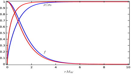
Figure 1: The electroweak monopole solution. The red and blue curves represent the singular Cho-Maison monopole and the regularized finite energy monopole obtained by (34) with $A=B=0$ and $n=6$.

With the ansatz we have the following equations of motion

$$\ddot{\rho}+\frac{2}{r}\dot{\rho}-\frac{1}{2r^{2}}f^{2}\rho=-\frac{1}{4}(B-A)^{2}\rho+\frac{\lambda}{2}\big{(}\rho^{2}-\rho_{0}^{2}\big{)}\rho,$$

$$\ddot{f}-\frac{1}{r^{2}}(f^{2}-1)f=\big{(}\frac{g^{2}}{4}\rho^{2}-A^{2}\big{)}~{}f,$$

$$\ddot{A}+\frac{2}{r}\dot{A}-\frac{2}{r^{2}}f^{2}A=\frac{g^{2}}{4}(A-B)~{}\rho^{2},$$

$$\ddot{B}+\frac{2}{r}\dot{B}=\frac{g^{\prime 2}}{4}(B-A)~{}^{2},$$ (29)

which has a singular solution

$$f=0,~{}~{}~{}\rho=\rho_{0}=\sqrt{2\mu^{2}/\lambda},$$

$$A_{\mu}^{\rm(em)}=-\frac{1}{e}(1-\cos\theta)\partial_{\mu}\varphi,~{}~{}~{}Z_{\mu}=0.$$ (30)

This describes the point monopole in Weinberg-Salam model which has the magnetic charge $4\pi/e$ (not $2\pi/e$).

With the boundary condition

$$\rho(0)=0,~{}~{}f(0)=1,~{}~{}A(0)=0,~{}~{}B(0)=b_{0},$$

$$\rho(\infty)=\rho_{0},~{}f(\infty)=0,~{}A(\infty)=B(\infty)=A_{0},$$ (31)

we can integrate (29). With $A=B=0$ we have the electroweak monopole with $q_{m}=4\pi/e$, but with non-trivial $A$ and $B$ we have the electroweak dyon which has the extra electric charge $q_{e}$ [2, 6]. The monopole and dyon solutions are shown in Fig. 1 and Fig. 2 in red curves.

There have been many studies of the electroweak monopole [7, 8, 9, 10, 11, 12, 13]. In particular, the stability of the Cho-Maison monopole has been established [14], and multi-monopole solutions have been discovered [15].

Since the solution contains the point singularity at the origin, it can be viewed as a hybrid between the Dirac monopole and the ’tHooft-Polyakov monopole. So at the classical level it carries an infinite energy, so that the mass is not determined. However, we could regularize the point singularity with the quantum correction at short distance. We could do this replacing the $U(1)_{Y}$ coupling constant $g^{\prime}$ to an effective coupling, or replacing the real electromagnetic coupling constant $e$ to an effective coupling [6].

To show this, we modify the Lagrangian (3) with a non-trivial $U(1)_{Y}$ permittivity ${\epsilon}(\rho)$ which depends on $\rho$,

$${\cal L}=-\frac{1}{2}(\partial_{\mu}\rho)^{2}-\frac{\lambda}{8}\big{(}\rho^{2}-\rho_{0}^{2}\big{)}^{2}-\frac{1}{4}{F^{\prime}}_{\mu\nu}^{2}$$

$$-\frac{1}{4}{\epsilon}(\rho)~{}G_{\mu\nu}^{2}-\frac{1}{2}|D^{\prime}_{\mu}W_{\nu}-D^{\prime}_{\nu}W_{\mu}|^{2}$$

$$-\frac{g^{2}}{4}{\rho}^{2}W_{\mu}^{*}W_{\mu}-\frac{1}{8}\rho^{2}(gA^{\prime}_{\mu}-g^{\prime}B_{\mu})^{2}$$

$$+igF^{\prime}_{\mu\nu}W_{\mu}^{*}W_{\nu}+\frac{g^{2}}{4}(W_{\mu}^{*}W_{\nu}-W_{\nu}^{*}W_{\mu})^{2}.$$ (32)

This retains the full $SU(2)\times U(1)_{Y}$ gauge symmetry. Moreover, when ${\epsilon}$ approaches to one asymptotically, it reproduces the standard model. But ${\epsilon}$ effectively changes the $U(1)_{Y}$ gauge coupling $g^{\prime}$ to the “running” coupling $\bar{g}^{\prime}=g^{\prime}/\sqrt{{\epsilon}}$. So, by making $\bar{g}^{\prime}$ infinite at the origin, we can regularize the Cho-Maison monopole [6].

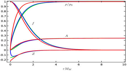
Figure 2: The electroweak dyon solution. The red and blue curves represent the singular Cho-Maison dyon and the regularized finite energy dyon obtained by (34), and the green curves represent the regularized dyon obtained by (38) with $n=6$. Notice that the blue and green curves are almost indistinguishable.

With this modification the dyon energy and the equation of motion are given by

$$E=4\pi\int_{0}^{\infty}dr\bigg{\{}\frac{{\epsilon}}{2g^{\prime 2}r^{2}}+\frac{1}{2}(r\dot{\rho})^{2}+\frac{\lambda}{8}r^{2}\big{(}\rho^{2}-\rho_{0}^{2}\big{)}^{2}$$

$$+\frac{1}{g^{2}}\big{(}\dot{f}^{2}+\frac{(f^{2}-1)^{2}}{2r^{2}}+f^{2}A^{2}\big{)}+\frac{1}{4}f^{2}\rho^{2}$$

$$+\frac{(r\dot{A})^{2}}{2g^{2}}+\frac{{\epsilon}(r\dot{B})^{2}}{2g^{\prime 2}}+\frac{r^{2}}{8}(A-B)^{2}\rho^{2}\bigg{\}},$$ (33)

and

$$\ddot{\rho}+\frac{2}{r}\dot{\rho}-\frac{f^{2}}{2r^{2}}\rho=\frac{\lambda}{2}(\rho^{2}-\rho_{0}^{2})\rho-\frac{1}{4}(A-B)^{2}\rho$$

$$+\frac{{\epsilon}^{\prime}}{2g^{\prime 2}}\big{(}\frac{1}{r^{4}}-\dot{B}^{2}\big{)},$$

$$\ddot{f}-\frac{f^{2}-1}{r^{2}}f=\big{(}\frac{g^{2}}{4}\rho^{2}-A^{2}\big{)}f,$$

$$\ddot{A}+\frac{2}{r}\dot{A}-\frac{2f^{2}}{r^{2}}A=\frac{g^{2}}{4}\rho^{2}(A-B),$$

$$\ddot{B}+2\big{(}\frac{1}{r}+\frac{{\epsilon}^{\prime}}{2{\epsilon}}\dot{\rho}\big{)}\dot{B}=-\frac{g^{\prime 2}}{4\epsilon}\rho^{2}(A-B),$$ (34)

where ${\epsilon}^{\prime}=d{\epsilon}/d\rho$. Assuming

$$\rho(r)=r^{\delta}(h_{0}+h_{1}r+...),$$

$${\epsilon}=\Big{(}\frac{\rho}{\rho_{0}}\Big{)}^{n}\big{[}c_{0}+c_{1}(\frac{\rho}{\rho_{0}})+...\big{]},$$ (35)

near the origin we can show that the energy becomes finite when $n>2$ [6].

We can integrate (34) with ${\epsilon}=(\rho/\rho_{0})^{n}$. The regularized monopole and dyon solutions with $n=6$ are shown in Fig. 1 and Fig. 2 in blue curves. Notice that asymptotically the regularized solutions look very much like the singular solutions, except that for the finite energy dyon solution $Z$ becomes zero at the origin. The regularized monopole energy with $n=6$ becomes

$$E\simeq 0.65\times\frac{4\pi}{e^{2}}M_{W}\simeq 7.20~{}{\rm TeV}.$$ (36)

This confirms that the ultraviolet regularization of the Cho-Maison dyon is indeed possible.

We could also regularize the monopole with the real electromagnetic permittivity. Consider the Lagrangian

$${\cal L^{\prime}}=-\frac{1}{2}(\partial_{\mu}\rho)^{2}-\frac{\lambda}{8}\big{(}\rho^{2}-\rho_{0}^{2}\big{)}^{2}-\frac{1}{4}{\bar{\epsilon}}(\rho){F_{\mu\nu}^{\rm(em)}}^{2}$$

$$-\frac{1}{2}\Big{|}\big{(}D_{\mu}^{\rm(em)}+ie\frac{g}{g^{\prime}}Z_{\mu}\big{)}W_{\nu}-\big{(}D_{\nu}^{\rm(em)}+ie\frac{g}{g^{\prime}}Z_{\nu}\big{)}W_{\mu}\Big{|}^{2}$$

$$+ie(F_{\mu\nu}^{\rm(em)}+\frac{g}{g^{\prime}}Z_{\mu\nu})W_{\mu}^{*}W_{\nu}+\frac{g^{2}}{4}(W_{\mu}^{*}W_{\nu}-W_{\nu}^{*}W_{\mu})^{2}$$

$$-\frac{1}{4}Z_{\mu\nu}^{2}-\frac{g^{2}}{4}\rho^{2}W_{\mu}^{*}W_{\mu}-\frac{g^{2}+g^{\prime 2}}{8}\rho^{2}Z_{\mu}^{2},$$ (37)

where ${\bar{\epsilon}}$ is the real non-vacuum electromagnetic permittivity. Just like (32) it retains all symmetries of the standard model, and asymptotically reduces to the standard model with ${\bar{\epsilon}}\rightarrow 1$. It has the dyon equation of motion

$$\ddot{\rho}+\frac{2}{r}\dot{\rho}-\frac{f^{2}}{2r^{2}}\rho=\frac{\lambda}{2}(\rho^{2}-\rho_{0}^{2})\rho-\frac{1}{4}(B-A)^{2}\rho$$

$$+\frac{{\bar{\epsilon}}^{\prime}}{2}\Big{(}\frac{1}{e^{2}r^{4}}-e^{2}(\frac{\dot{A}}{g^{2}}+\frac{\dot{B}}{g^{\prime 2}})^{2}\Big{)},$$

$$\ddot{f}-\frac{f^{2}-1}{r^{2}}f=\big{(}\frac{g^{2}}{4}\rho^{2}-B^{2}\big{)}f,$$

$$\ddot{A}+\frac{2}{r}\dot{A}+e^{2}\frac{{\bar{\epsilon}}^{\prime}}{{\bar{\epsilon}}}\dot{\rho}\big{(}\frac{\dot{A}}{g^{2}}+\frac{\dot{B}}{g^{\prime 2}}\big{)}-\frac{2e^{2}}{g^{2}}\big{(}\frac{g^{2}}{g^{\prime 2}}+\frac{1}{{\bar{\epsilon}}}\big{)}\frac{f^{2}}{r^{2}}A$$

$$=-\frac{g^{2}}{4}\rho^{2}(B-A),$$

$$\ddot{B}+\frac{2}{r}\dot{B}+e^{2}\frac{{\bar{\epsilon}}^{\prime}}{{\bar{\epsilon}}}\dot{\rho}\big{(}\frac{\dot{A}}{g^{2}}+\frac{\dot{B}}{g^{\prime 2}}\big{)}+\frac{2e^{2}}{g^{2}}\big{(}1-\frac{1}{{\bar{\epsilon}}}\big{)}\frac{f^{2}}{r^{2}}A$$

$$=\frac{g^{\prime 2}}{4}(B-A)\rho^{2}.$$ (38)

To integrate it out and find a finite energy solution we have to choose a proper boundary condition.

Now, with

$${\bar{\epsilon}}={\epsilon}_{0}+{\epsilon}_{1},$$

$${\epsilon}_{0}=\frac{g^{\prime 2}}{g^{2}+g^{\prime 2}},~{}~{}~{}{\epsilon}_{1}={\epsilon}_{1}(\rho),$$ (39)

the dyon energy becomes

$$E=4\pi\int_{0}^{\infty}dr\bigg{\{}\frac{1}{2e^{2}r^{2}}\Big{(}{\epsilon}_{0}(f^{2}-1)^{2}+{\epsilon}_{1}\Big{)}+\frac{1}{2}(r\dot{\rho})^{2}$$

$$+\frac{\lambda r^{2}}{8}\big{(}\rho^{2}-\rho_{0}^{2}\big{)}^{2}+\frac{1}{g^{2}}\dot{f}^{2}+\frac{1}{4}f^{2}\rho^{2}+\frac{f^{2}A^{2}}{g^{2}}$$

$$+\frac{r^{2}}{8}(A-B)^{2}\rho^{2}+\frac{r^{2}(A^{\prime}-B^{\prime})^{2}}{2(g^{2}+g^{\prime 2})}$$

$$+({\epsilon}_{0}+{\epsilon}_{1})\frac{e^{2}r^{2}}{2}\big{(}\frac{A^{\prime}}{g^{2}}+\frac{B^{\prime}}{g^{\prime 2}}\big{)}^{2}\bigg{\}}.$$ (40)

This shows that the energy can be made finite with $f(0)=1$, when ${\epsilon}_{1}$ approaches to zero quickly enough near the origin.

We can integrate (38) with

$${\bar{\epsilon}}={\epsilon}_{0}+(1-{\epsilon}_{0})\Big{(}\frac{\rho}{\rho_{0}}\Big{)}^{n}.$$ (41)

With $A=B=0$, we have the monopole solution shown in Fig. 1 in red curves, and the dyon solution shown in Fig. 2 with non-trivial $A$ and $B$ in blue curves.

Remarkably, for the monopole solutions for the two equations (34) and (38) become identical. To see this notice that with

$${\bar{\epsilon}}^{\prime}=\frac{\partial}{\partial\rho}\Big{[}{\epsilon}_{0}+(1-{\epsilon}_{0})\big{(}\frac{\rho}{\rho_{0}}\big{)}^{n}\Big{]}=\frac{g^{2}}{g^{2}+g^{\prime 2}}\frac{\partial}{\partial\rho}\Big{(}\frac{\rho}{\rho_{0}}\Big{)}^{n},$$

$$\frac{{\bar{\epsilon}}^{\prime}}{e^{2}}=\frac{1}{g^{\prime 2}}\frac{\partial}{\partial\rho}\Big{(}\frac{\rho}{\rho_{0}}\Big{)}^{n}=\frac{1}{g^{\prime 2}}{\epsilon}^{\prime},$$ (42)

the monopole equation of (38) with $A=B=0$ becomes

$$\ddot{\rho}+\frac{2}{r}\dot{\rho}-\frac{f^{2}}{2r^{2}}\rho=\frac{\lambda}{2}(\rho^{2}-\rho_{0}^{2})\rho+\frac{{\epsilon}^{\prime}}{2g^{\prime 2}r^{4}},$$

$$\ddot{f}-\frac{f^{2}-1}{r^{2}}f=\frac{g^{\prime 2}}{4}\rho^{2}f.$$ (43)

This is identical to the monopole equation (34) with $A=B=0$. Moreover, with

$$\frac{1}{e^{2}}{\epsilon}_{0}=\frac{1}{e^{2}}\frac{g^{\prime 2}}{g^{2}+g^{\prime 2}}=\frac{1}{g^{2}},$$

$$\frac{1}{e^{2}}(1-{\epsilon}_{0})=\frac{1}{e^{2}}\frac{g^{2}}{g^{2}+g^{\prime 2}}=\frac{1}{g^{\prime 2}},$$ (44)

the monopole energy (40) with $A=B=0$ becomes identical to the monopole energy given by (33) with $A=B=0$. This assures that the two monopole solutions regularized by the hypercharge renormalization and the real electric charge renormalization are indeed identical to each other [12]. For the dyon, however, the two equations (34) and (38) give different solutions. This is evident in Fig. 2.

Of course, the above regularization is not the only way to regularize the Cho-Maison monopole. One could regularize the monopole replacing the $U(1)_{Y}$ part by the Bonn-Infeld Lagrangian [8, 10], or by other (logarithmic or exponential) non-linear extensions of the $U(1)_{Y}$ part in (3) [13]. For example, in the Bonn-Infeld modification the monopole mass is estimated to be around 11.6 TeV, and in the logarithmic and exponential extensions the mass is estimated to be around 8.7 TeV and 7.9 TeV.

This, with the above analysis of the regularization by charge renormalization, strongly suggests that the monopole could also be regularized replacing the real Maxwell part (not the hypercharge part) by the Bonn-Infeld Lagrangian or by the nonlinear extensions in (19).

IV Electroweak String Configuration

As we have pointed out, the standard model has two $\pi_{1}(S^{1})$ topology, so that it should have strings. To see this notice that the core of the electroweak monopole is the Dirac type singular monopole shown in (30). If this is so, we could also expect the singular electroweak string made of monopole-antimonopole pair infinitely separated apart, which can be expressed as

$$\rho=\rho_{0},~{}~{}~{}A_{\mu}^{\rm(em)}=\frac{2n}{e}~{}\partial_{\mu}{\varphi},$$

$$W_{\mu}=0,~{}~{}~{}Z_{\mu}=0,$$ (45)

which carries the quantized magnetic flux $4\pi n/e$. This strongly implies that the string made of the Cho-Maison monopole-antimonopole pair could exist.

To obtain such solution we consider the following string ansatz in the cylindrical coordinates $(t,r,\varphi,z)$,

$$\phi=\frac{1}{\sqrt{2}}\rho(r)\xi,~{}~{}~{}\xi=\left(\begin{array}[]{cc}-\sin\dfrac{\alpha(r)}{2}~{}\exp(-in{\varphi})\\ \cos\dfrac{\alpha(r)}{2}\end{array}\right),$$ (48)

$${\vec{A}}_{\mu}=\frac{n}{g}\big{(}A(r)+1-\cos\alpha(r)\big{)}\partial_{\mu}{\varphi}~{}\hat{n}$$

$$+\frac{1}{g}\big{(}f(r)-1\big{)}~{}\hat{n}\times\partial_{\mu}\hat{n},$$

$$B_{\mu}=\frac{m}{g^{\prime}}B~{}\partial_{\mu}{\varphi},$$ (49)

where $m$ and $n$ are integers. To understand the physical meaning of the ansatz we notice that, with the $U(1)_{Y}$ gauge transformation

$$\xi\rightarrow\exp\big{(}-i(m-\frac{n}{2}){\varphi}\big{)}\xi$$

$$=\exp(-im{\varphi})\left(\begin{array}[]{cc}-\sin\dfrac{\alpha(r)}{2}~{}\exp(-i\dfrac{n}{2}{\varphi})\\ \cos\dfrac{\alpha(r)}{2}~{}\exp(i\dfrac{n}{2}{\varphi})\end{array}\right),$$ (52)

$$B_{\mu}\rightarrow\frac{1}{g^{\prime}}\Big{(}m(B-2)+n\Big{)}~{}\partial_{\mu}{\varphi},$$ (53)

the ansatz acquires the following form

$$\phi=\frac{1}{\sqrt{2}}\rho(r)\xi,$$

$$\xi=\exp(-im{\varphi})\left(\begin{array}[]{cc}~{}-\sin\dfrac{\alpha(r)}{2}~{}\exp(-i\dfrac{n}{2}{\varphi})\\ \cos\dfrac{\alpha(r)}{2}~{}\exp(i\dfrac{n}{2}{\varphi})\end{array}\right),$$ (56)

$${\vec{A}}_{\mu}=\frac{n}{g}\big{(}A(r)+1-\cos\alpha(r)\big{)}\partial_{\mu}{\varphi}~{}\hat{n}$$

$$+\frac{1}{g}\big{(}f(r)-1\big{)}~{}\hat{n}\times\partial_{\mu}\hat{n},$$

$$B_{\mu}=\frac{1}{g^{\prime}}\Big{(}m(B-2)+n\Big{)}~{}\partial_{\mu}{\varphi}.$$ (57)

In this expression the meaning of the integers $m$ and $n$ becomes clear. They represent the winding numbers of the $\pi_{1}(S^{1})$ topology of $U(1)_{Y}$ and $U(1)$ subgroup of $SU(2)$.

Notice, however, that in the ansatz (57) $\xi$ becomes single valued under the $2\pi$ rotation along the z-axis only when $n$ becomes even integers. This is because the gauge transformation (53) becomes singular when $n$ becomes odd integers. This means that for $n$ to represent the $\pi_{1}(S_{1})$ topology of the $U(1)$ subgroup of SU(2) it must be even integers. This point will become important later.

With (49) we have

$$\hat{n}=-\xi^{\dagger}{\vec{\sigma}}\xi=\left(\begin{array}[]{ccc}\sin\alpha\cos n{\varphi}\\ \sin\alpha\sin n{\varphi}\\ \cos\alpha\end{array}\right),$$ (61)

$$C_{\mu}\simeq-\frac{2i}{g}\xi^{\dagger}\partial_{\mu}\xi=-\frac{n}{g}(1-\cos\alpha)~{}\partial_{\mu}{\varphi},$$

$$A^{\prime}_{\mu}=\frac{n}{g}A~{}\partial_{\mu}{\varphi}.$$ (62)

This means that the ansatz, in terms of the physical field, becomes

$$\rho=\rho(r),$$

$$A_{\mu}^{(\rm em)}=e\Big{(}\frac{n}{g^{2}}A+\frac{m}{g^{\prime 2}}B\Big{)}~{}\partial_{\mu}{\varphi},$$

$$W_{\mu}=\frac{i}{g}\frac{f}{\sqrt{2}}\exp(in{\varphi})~{}(\partial_{\mu}\alpha+in\sin\alpha\partial_{\mu}{\varphi}),$$

$$Z_{\mu}=\frac{1}{\sqrt{g^{2}+g^{\prime 2}}}\big{(}nA-mB\big{)}~{}\partial_{\mu}{\varphi}.$$ (63)

We can confirm this writing the ansatz in the “unitary” (or “physical”) gauge with the following gauge transformation

$$\xi\rightarrow U\xi=\left(\begin{array}[]{cc}0\\ 1\end{array}\right),$$ (66)

$$U=\left(\begin{array}[]{cc}\cos\dfrac{\alpha}{2},&\sin\dfrac{\alpha}{2}\exp(-in{\varphi})\\ -\sin\dfrac{\alpha}{2}\exp(in{\varphi}),&\cos\dfrac{\alpha}{2}\end{array}\right).$$ (69)

With this gauge transformation the ansatz changes to

$${\vec{A}}_{\mu}\rightarrow\frac{1}{g}\left(\begin{array}[]{ccc}-f(n\cos(n\varphi)\sin\alpha~{}\partial_{\mu}{\varphi}+\sin(n\varphi)\partial_{\mu}\alpha)\\ -f(n\sin(n\varphi)\sin\alpha~{}\partial_{\mu}{\varphi}-\cos(n\varphi)\partial_{\mu}\alpha)\\ nA~{}\partial_{\mu}{\varphi}\end{array}\right),$$ (73)

$$B_{\mu}\rightarrow\frac{m}{g^{\prime}}B~{}\partial_{\mu}{\varphi}.$$ (74)

From this we reproduce (63).

So, when

$$nA=mB$$ (75)

the ansatz describes the electromagnetic string

$$A_{\mu}^{(\rm em)}=\frac{n}{e}A~{}\partial_{\mu}{\varphi},$$

$$Z_{\mu}=0.$$ (76)

But when

$$ng^{\prime 2}A+mg^{2}B=0,$$ (77)

the ansatz describes the Z boson string

$$A_{\mu}^{(\rm em)}=0,$$

$$Z_{\mu}=-m\frac{\sqrt{g^{2}+g^{\prime 2}}}{g^{\prime 2}}B~{}\partial_{\mu}{\varphi}=-\frac{m}{e}B~{}\cot~{}\theta_{\rm w}~{}\partial_{\mu}{\varphi}.$$ (78)

This confirms that the ansatz is able to describe both electromagnetic and Z boson strings.

With the ansatz (49) we have the following string equations of motion from (21),

$$\ddot{\rho}+\frac{\dot{\rho}}{r}-\frac{1}{4}\Big{(}f^{2}\dot{\alpha}^{2}+\frac{n^{2}f^{2}\sin^{2}\alpha+(nA-mB)^{2}}{r^{2}}\Big{)}~{}\rho=\frac{\lambda}{2}\rho(\rho^{2}-\rho_{0}^{2}),$$

$$f\rho\Big{[}\ddot{\alpha}+\Big{(}\frac{1}{r}+2\frac{\dot{\rho}}{\rho}+\frac{\dot{f}}{f}\Big{)}\dot{\alpha}-\frac{n(mB+n)\sin\alpha}{r^{2}}\Big{]}=0,$$

$$n\Big{(}\ddot{A}-\frac{\dot{A}}{r}\Big{)}+nf^{2}\Big{(}\sin\alpha(\ddot{\alpha}-\frac{\dot{\alpha}}{r}+3\frac{\dot{f}}{f}\dot{\alpha})+(2\cos\alpha-A-1)\dot{\alpha}^{2}\Big{)}=\frac{g^{2}}{4}\rho^{2}\big{(}nA-mB\big{)},$$

$$\sin\alpha\Big{(}\ddot{f}-\frac{\dot{f}}{r}-(f^{2}+1)f\dot{\alpha}^{2}\Big{)}+(\cos\alpha-A-1)f\Big{(}\ddot{\alpha}-\frac{\dot{\alpha}}{r}\Big{)}+(2\cos\alpha-A-1)\dot{\alpha}\dot{f}-2f\dot{A}\dot{\alpha}=\frac{g^{2}}{4}\rho^{2}f\sin\alpha,$$

$$m\big{(}\ddot{B}-\frac{\dot{B}}{r}\big{)}=-\frac{g^{\prime 2}}{4}\rho^{2}\big{(}nA-mB\big{)},$$

$$n^{2}\Big{[}(A+1)\sin\alpha\dot{f}-\Big{(}f^{2}\sin^{2}\alpha-(A+1)(\cos\alpha-A-1)\Big{)}f\dot{\alpha}-f\sin\alpha\dot{A}\Big{]}=\frac{g^{2}}{4}r^{2}\rho^{2}f\dot{\alpha}.$$ (79)

Notice that, in spite of the fact that we have 5 variables in the ansatz (49), here we have 6 equations of motion. So in principle, we could have no solution. As we will see, however, the equation does allow us to have solutions.

V Electromagnetic String: Quantized Magnetic Vortex

From (79) we can obtain the electromagnetic string solution made of quantized magnetic flux. With (75) the equation reduces to

$$\ddot{\rho}+\frac{\dot{\rho}}{r}-\frac{f^{2}}{4}\Big{(}\dot{\alpha}^{2}+\frac{n^{2}\sin^{2}\alpha}{r^{2}}\Big{)}~{}\rho=\frac{\lambda}{2}\rho(\rho^{2}-\rho_{0}^{2}),$$

$$f\rho\Big{[}\ddot{\alpha}+\Big{(}\frac{1}{r}+2\frac{\dot{\rho}}{\rho}+\frac{\dot{f}}{f}\Big{)}\dot{\alpha}-\frac{n^{2}\sin\alpha(A+1)}{r^{2}}\Big{]}=0,$$

$$f^{2}\Big{(}\sin\alpha(\ddot{\alpha}-\frac{\dot{\alpha}}{r}+3\frac{\dot{f}}{f}\dot{\alpha})+(2\cos\alpha-A-1)\dot{\alpha}^{2}\Big{)}=0,$$

$$\sin\alpha\Big{(}\ddot{f}-\frac{\dot{f}}{r}-(f^{2}+1)f\dot{\alpha}^{2}\Big{)}+(\cos\alpha-A-1)f\Big{(}\ddot{\alpha}-\frac{\dot{\alpha}}{r}\Big{)}$$

$$+(2\cos\alpha-A-1)\dot{\alpha}\dot{f}-2f\dot{A}\dot{\alpha}=\frac{g^{2}}{4}\rho^{2}f\sin\alpha,$$

$$\ddot{A}-\frac{\dot{A}}{r}=0,$$

$$n^{2}\Big{[}\sin\alpha\Big{(}(A+1)\dot{f}-\dot{A}f\Big{)}$$

$$-\Big{(}f^{2}\sin^{2}\alpha-(A+1)(\cos\alpha-A-1)\Big{)}f\dot{\alpha}\Big{]}$$

$$=\frac{1}{4}g^{2}r^{2}\rho^{2}f\dot{\alpha}.$$ (80)

This, with

$$A=-1,~{}~{}~{}\alpha=\frac{\pi}{2}$$ (81)

reduces to

$$\ddot{\rho}+\frac{\dot{\rho}}{r}-\frac{n^{2}}{4}\frac{f^{2}}{r^{2}}~{}\rho=\frac{\lambda}{2}\rho(\rho^{2}-\rho_{0}^{2}),$$

$$\ddot{f}-\frac{\dot{f}}{r}-\frac{g^{2}}{4}\rho^{2}f=0.$$ (82)

Notice that this is precisely the equation which describes the Abrikosov-Nielsen-Olesen (ANO) vortex [25]. But here we are not looking for the ANO vortex, but an electromagnetic vortex described by (76).

Clearly (82) has the naked singular electromagnetic string solution given by

$$\rho=\rho_{0},~{}~{}~{}~{}~{}f=0,$$

$$A_{\mu}^{(\rm em)}=-\frac{n}{e}\partial_{\mu}{\varphi},$$ (83)

which becomes precisely the magnetic vortex solution that we predicted in (45). The only difference is that here the string carries the quantized magnetic flux $2\pi n/e$, not $4\pi n/e$. So only when $n$ becomes even, the above solution describes the predicted solution.

To understand the situation we have to remember that only when $n$ becomes even integers it represents the $\pi_{1}(S^{1})$ topology of the $U(1)$ subgroup of $SU(2)$. This is because the period of the $U(1)$ subgroup of $SU(2)$ is $4\pi$, not $2\pi$. So the above solution indeed describes the string solution made of the monopole-antimonopole pair infinitely separated apart with the $\pi_{1}(S^{1})$ topology of the $U(1)$ subgroup of $SU(2)$, when $n$ becomes even. But what is interesting here is that we have the electromagnetic string even when $n$ is odd, which can not be interpreted as the string made by monopole-antimonopole pair.

We can solve (82) with the boundary condition

$$\rho(0)=0,~{}~{}~{}\rho(\infty)=\rho_{0},$$

$$f(0)=1,~{}~{}~{}f(\infty)=0,$$ (84)

and obtain the singular but dressed quantized string solution shown in Fig. (3), dressed by Higgs and W boson. At the origin $\rho$ and $f$ can be expressed by

$$\rho\simeq r^{\delta}(a_{1}+a_{2}r+...),~{}~{}~{}\delta=|n|/2,$$

$$f\simeq 1+b_{1}r^{2}+...,$$ (85)

so that the solution becomes regular.

Figure 3: The Higgs and W boson configurations of the quantized magnetic vortex solutions with $A=-1$ and $\alpha=\pi/2$. The black and blue curves represent solutions with $n=1$ and $n=2$, respectively. The dotted curves represent the energy densities of the Higgs and W bosons.

Asymptotically they have the form of modified second kind Bessel function

$$\rho=\rho_{0}-K_{0}(\sqrt{\lambda\rho_{0}}r)$$

$$\simeq\rho_{0}-\sqrt{\frac{\pi}{2\sqrt{\lambda\rho_{0}}r}}\exp(-\sqrt{\lambda\rho_{0}}r)\left(1-\frac{1}{8\sqrt{\lambda\rho_{0}}r}+...\right),$$

$$f=rK_{1}\left(\frac{g\rho_{0}}{2}r\right)$$

$$\simeq\sqrt{\frac{\pi r}{g\rho_{0}}}\exp\left(-\frac{g\rho_{0}}{2}r\right)\left(1+\frac{3}{4g\rho_{0}r}+...\right)$$ (86)

so that they have the exponential damping set by the Higgs and W boson mass

$$\rho\simeq\rho_{0}-\sqrt{\frac{\pi}{2m_{H}r}}\exp(-m_{H}r)+...,$$

$$f\simeq\sqrt{\frac{\pi r}{2m_{W}}}\exp(-m_{W}r)+...,$$ (87)

similar to the Cho-Maison monopole [2]. This confirms that the dressed string solution is nothing but the string made of the Cho-Maison monopole-antimonopole pair infinitely separated apart.

To understand the meaning of this solution, remember that the electromagnetic field of the solution is given by

$$A_{\mu}^{(\rm em)}=-\frac{n}{e}\partial_{\mu}{\varphi},$$ (88)

which has the quantized magnetic flux along the $z$-axis,

$$\Phi=\displaystyle\int{\vec{B}}\cdot d\vec{S}=\displaystyle\int_{r=\infty}A_{\mu}^{\rm(em)}dx^{\mu}=-\frac{2\pi n}{e}.$$ (89)

So the solution describes the singular quantized magnetic flux dressed by the Higgs and W bosons in the standard model. Notice that, although the magnetic field ${\vec{B}}$ vanishes everywhere except at the origin, it has a 2-dimensional $\delta$-function singularity at the origin. Clearly this string singularity is topological, whose quantized magnetic flux represents the non-trivial winding number of $\pi_{1}(S^{1})$. This means that, just like the Cho-Maison monopole, the solution has infinite magnetic energy (per unit length).

For the monopole, it is well known that the magnetic point singularity which makes the energy infinite can be regularized by various methods, for example by the vacuum polarization or by the gravitational interaction [6, 9, 11, 12]. One might wonder if similar methods could also make the string energy finite. This is a very interesting question to be studied further.

Excluding the singular magnetic field, the energy (per unit length) of the Higgs and W boson is given by

$$E=2\pi\displaystyle\int\Big{[}\frac{\dot{\rho}^{2}}{2}+\frac{\lambda}{8}(\rho^{2}-\rho_{0}^{2})^{2}+\frac{n^{2}\dot{f}^{2}}{2g^{2}r^{2}}$$

$$+\frac{n^{2}f^{2}\rho^{2}}{8r^{2}}\Big{]}rdr.$$ (90)

This is the same energy functional of Abrikosov-Nielsen-Olesen vortex which has the following BPS bound,

$$E=2\pi\displaystyle\int\Big{[}\frac{1}{2g^{2}r}\Big{(}n\dot{f}+\frac{g\sqrt{\lambda}}{2}r(\rho^{2}-\rho^{2}_{0})\Big{)}^{2}$$

$$+\frac{r}{2}(\dot{\rho}-\frac{nf\rho}{2r})^{2}-\frac{n\sqrt{\lambda}}{2g}\dot{f}(\rho^{2}-\rho^{2}_{0})+\frac{1}{2}nf\rho\dot{\rho}\Big{]}dr$$

$$\geq 2\pi\displaystyle\int\Big{[}\frac{\lambda}{4}r(\rho^{2}-\rho_{0}^{2})^{2}+\frac{n^{2}f^{2}\rho^{2}}{4r}\Big{]}dr,$$ (91)

when we have the Bogomolny equation

$$\dot{\rho}=\frac{nf\rho}{2r},$$

$$n\dot{f}=-\frac{g\sqrt{\lambda}}{2}r(\rho^{2}-\rho_{0}^{2}).$$ (92)

In the BPS limit (with $\lambda=0$) this has the trivial solution (83). For $\lambda\neq 0$ the numerical BPS vortex solution is shown in Fig. 4.

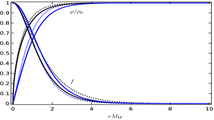
Figure 4: The BPS string solutions with $A=-1$ and $\alpha=\pi/2$. The black and blue curve represent solutions with $n=1$ and $n=2$, respectively. For comparison the singular string solutions in Fig. 3 are plotted correspondingly with dotted black lines and blue lines.

As we have already pointed out, (76) is the equation for the ANO vortex. So, as far as $\rho$ and $f$ are concerned, they describe the well known ANO vortex. The difference here is that we also have the singular quantized magnetic vortex (88). If so, one might wonder what will happen if we remove the string singularity of (88) with a gauge transformation.

To answer this we consider the gauge transformation

$$A_{\mu}^{(\rm em)}\rightarrow{A^{\prime}}_{\mu}^{(\rm em)}=A_{\mu}^{\rm(em)}+\frac{n}{e}\partial_{\mu}{\varphi}=0,$$

$$W_{\mu}\rightarrow W_{\mu}^{\prime}=\exp\big{(}-in{\varphi}\big{)}W_{\mu}=-\frac{n}{g}\frac{f}{\sqrt{2}}\partial_{\mu}{\varphi}.$$ (93)

This is the singular gauge transformation which removes the string singularity and changes the $\pi_{1}(S^{1})$ topology of the string. Obviously this changes the physical content of the solution. But mathematically there is nothing wrong with this gauge transformation, in the sense that it keeps ${A^{\prime}}_{\mu}^{(\rm em)}$ and $W_{\mu}^{\prime}$ as a qualified solution after the gauge transformation. So, after the gauge they become physically a different solution. This tells that the standard model has a electromagnetically neutral string solution made of Higgs and W bosons described by Fig. 3 which does not carry any magnetic flux, whose energy is finite.

The reason why such a solution is possible is that, in the absence of $A_{\mu}^{\rm(em)}$ and $Z_{\mu}$, the Lagrangian (19) reduces to the Landau-Ginzburg theory with the gauge potential $W^{\prime}_{\mu}$ when $W_{\mu}$ becomes $W^{\prime}_{\mu}$. So it must have the ANO vortex solution, which is exactly the solution discussed above. In fact we can easily see that the equation (82) is exactly the equation for the ANO vortex. In the literature this solution is known as the W string [20, 21]. This tells that the electromagnetic vortex solution in the standard model is nothing but the W string which has the topological singular quantized magnetic flux at the core.

Notice that to have the above quantized magnetic vortex we do not have to require $\alpha$ to be $\pi/2$. Actually $\alpha$ can be any constant, as far as $\sin\alpha\neq 0$. In fact, with $A=-1$ and $\sin\alpha\neq 0$, (80) reduces to

$$\ddot{\rho}+\frac{\dot{\rho}}{r}-\frac{n^{2}}{4}\frac{f^{2}}{r^{2}}\sin^{2}\alpha~{}\rho=\frac{\lambda}{2}\rho(\rho^{2}-\rho_{0}^{2}),$$

$$\sin\alpha\Big{(}\ddot{f}-\frac{1}{r}\dot{f}-\frac{g^{2}}{4}\rho^{2}f\Big{)}=0.$$ (94)

Obviously this (with the replacement of $f\sin\alpha$ to $f$) is mathematically identical to (82), and has essentially the same quantized magnetic vortex solutions.

VI Z string

To obtain the Z string solution, notice that (77) reduces the string equation (79) to

$$\ddot{\rho}+\frac{\dot{\rho}}{r}-\frac{1}{4}\Big{(}f^{2}\dot{\alpha}^{2}+n^{2}\frac{f^{2}\sin^{2}\alpha+A^{2}\sec^{4}\theta_{W}}{r^{2}}\Big{)}~{}\rho$$

$$=\frac{\lambda}{2}\rho(\rho^{2}-\rho_{0}^{2}),$$

$$f\rho\Big{[}\ddot{\alpha}+\Big{(}\frac{1}{r}+2\frac{\dot{\rho}}{\rho}+\frac{\dot{f}}{f}\Big{)}\dot{\alpha}-n^{2}\frac{(1-A\tan^{2}\theta_{W})\sin\alpha}{r^{2}}\Big{]}=0,$$

$$\Big{(}\ddot{A}-\frac{\dot{A}}{r}\Big{)}+f^{2}\Big{(}\sin\alpha(\ddot{\alpha}-\frac{\dot{\alpha}}{r}+3\frac{\dot{f}}{f}\dot{\alpha})$$

$$+(2\cos\alpha-A-1)\dot{\alpha}^{2}\Big{)}=\frac{g^{\prime 2}+g^{2}}{4}\rho^{2}A,$$

$$\sin\alpha\Big{(}\ddot{f}-\frac{\dot{f}}{r}-(f^{2}+1)f\dot{\alpha}^{2}\Big{)}+(\cos\alpha-A-1)f\Big{(}\ddot{\alpha}-\frac{\dot{\alpha}}{r}\Big{)}$$

$$+(2\cos\alpha-A-1)\dot{\alpha}\dot{f}-2f\dot{A}\dot{\alpha}=\frac{g^{2}}{4}\rho^{2}f\sin\alpha,$$

$$\big{(}\ddot{A}-\frac{\dot{A}}{r}\big{)}=\frac{g^{\prime 2}+g^{2}}{4}\rho^{2}A,$$

$$n^{2}\Big{[}(A+1)\sin\alpha\dot{f}-f\sin\alpha\dot{A}$$

$$-\Big{(}f^{2}\sin^{2}\alpha-(A+1)(\cos\alpha-A-1)\Big{)}f\dot{\alpha}\Big{]}$$

$$=\frac{1}{4}g^{2}r^{2}\rho^{2}f\dot{\alpha}.$$ (95)

where $\theta_{W}$ is the Weinberg angle.

When $f=0$, this simplifies to

$$\ddot{\rho}+\frac{\dot{\rho}}{r}-n^{2}\frac{Z^{2}}{r^{2}}\rho=\frac{\lambda}{2}\rho(\rho^{2}-\rho_{0}^{2}),$$

$$\ddot{Z}-\frac{\dot{Z}}{r}-\frac{g^{2}}{4}\rho^{2}Z=0.$$ (96)

where

$$Z(r)=\frac{g^{2}+g^{\prime 2}}{2g^{\prime 2}}A(r)=-\frac{m}{2n}\frac{\cos^{2}\theta_{W}}{\sin^{4}\theta_{W}}~{}B(r).$$ (97)

Clearly this is mathematically identical to the equation (82) which describes the well known ANO vortex [25]. The reason for this is that the standard model reduces to Landau-Ginzburg theory in the absence of the $W$ boson and electromagnetic field, which is well known to admit the ANO vortex solution. This means that the standard model has another string solution known as the Z string in the literature [20, 21].

We can solve (96) with the boundary condition

$$\rho(0)=0,~{}~{}~{}\rho(\infty)=\rho_{0},$$

$$Z(0)=1,~{}~{}~{}Z(\infty)=0.$$ (98)

But here we can choose a more general boundary condition

$$\rho(0)=\frac{d\rho}{dr}(0)=...=\frac{d^{k-1}\rho}{d^{k-1}r}(0)=0,$$

$$\frac{d^{k}\rho}{d^{k}r}(0)\neq 0,~{}~{}~{}\rho(\infty)=\rho_{0},$$

$$Z(0)=\pm\frac{k}{n},~{}~{}~{}Z(\infty)=0,$$ (99)

and integrate (96) to obtain the Z string solution given by

$$\rho=\rho(r),$$

$$A_{\mu}^{(\rm em)}=0,~{}~{}~{}W_{\mu}=0,$$

$$Z_{\mu}=-\frac{m}{e}B(r)~{}\cot\theta_{W}\partial_{\mu}{\varphi}.$$ (100)

The solution for $k=1$ and $k=2$ (with $n=1$) are shown in Fig. 5. This, of course, is the well known Z string [20, 21]. This confirms that the Z string is nothing but the ANO string embedded in the standard model.

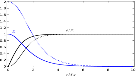
Figure 5: The Z boson string solution for $k=1$ (solid curves) and $k=2$ (dotted curves) with $n=1$.

Before we close this section it is worth mentioning another string in the standard model known as the Nambu string [19]. To understand the Nambu string we notice that, with $\phi=(0,\eta)$, ${\vec{A}}_{\mu}=(0,0,A_{\mu})$, and $B_{\mu}=0$, the Weinberg-Salam Lagrangian (1) reduces to

$${\cal L}=-|D_{\mu}\eta|^{2}-\frac{\lambda}{2}\big{(}|\eta|^{2}-\frac{\mu^{2}}{\lambda}\big{)}^{2}-\frac{1}{4}F_{\mu\nu}^{2},$$

$$D_{\mu}\eta=\big{(}\partial_{\mu}+i\frac{g}{2}A_{\mu}\big{)}\eta.$$ (101)

This is nothing but the Landau-Ginzburg Lagrangian which admits the ANO vortex, which carries the quantized magnetic flux $4\pi n/g$ (or $4\pi n\sin\theta_{\rm w}/e$) of the gauge filed $A_{\mu}$. This vortex is known as the Nambu string. But physically this vortex is a mixed string made of the electromagnetic and Z strings, because $A_{\mu}$ is a combination of $A_{\mu}^{\rm(em)}$ and $Z_{\mu}$. So this string carries fractional (electro)magnetic and Z flux given by $(4\pi n/e)\times\sin^{2}\theta_{\rm w}$ and $(4\pi n/e)\times\sin\theta_{\rm w}\cos\theta_{\rm w}$. This is because $A_{\mu}$ is given by $A_{\mu}^{\rm(em)}\sin\theta_{\rm w}$ and $Z_{\mu}\cos\theta_{\rm w}$.

At this point one might worry about the stability of the above strings. This is ligitemate because, if they are not stable, they can not be treated as real. Fortunately we do not have to worry about this, since there is a simple and natural way to make them stable. Indeed we can always make them topologically stable by making them a twisted vortex ring, making them periodic and join both ends together, endowing the knot topology $\pi_{3}(S^{2})$ [26, 27].

In fact it is well known that the Faddeev-Niemi knot in Skyrme theory can be interpreted as the twisted vortex ring (i.e., the twisted baby skyrmion) made this way. Of course, this type of twisted vortex ring is, strictly speaking, not a string. But in all practical purpose they can be treated as a string, as far as we make them long enough. This assures us to tell confidently that the standard model does have the above Nambu string.

VII Discussion

In this work we have discussed all possible string type solutions in the standard model. We have shown that there are basically two types of topological string solutions in the standard model. The reason for this two types of solutions comes from the fact that the Weinberg-Salam Lagrangian contains two $U(1)$, the $U(1)$ subgroup of $SU(2)$ and $U(1)_{Y}$, which allows two different $\pi_{1}(S^{1})$ string topology.

The string solutions we have discussed include the well known Nambu string, Z string, and W string [19, 20, 21]. The new solution here is the electromagnetic string which has the quantized $4\pi n/e$ magnetic flux which connects the Cho-Maison monopole-antimonopole pair infinitely separated apart. Actually there are two of them, a naked magnetic flux string and a dressed one which has the Higgs and W boson profiles. The existence of such quantized magnetic flux strings in the standard model, of course, is not surprising because the Cho-Maison monopole predicts this.

In this connection it should be mentioned that a finite length quantized magnetic flux made of the Cho-Maison monopole-antimonopole pair has recently been constructed numerically [28]. It has the pole separation length around $8.2/M_{W}$ and has the magnetic dipole moment roughly $8.6/M_{W}$. This is very interesting. The main difference between this and our solution is that this numerical string has a finite length, so that become metastable. This is because the monopole-antimonopole pair could annihilate each other. In comparison, ours is classically stable because it has infinite length. On the other hand the existence of the metastable solution made of Cho-Maison monopole-antimonopole pair strongly supports the existence of our string. With this we may conclude that the electromagnetic string made of quantized magnetic flux must exist in the standard model.

The Cho-Maison monopole in the standard model has deep implications in physics, in particular, in cosmology. When coupled to gravity, the electroweak monopole turns to Reissner-Nordstrom type magnetic black hole which could become the seed of the stellar objects and galaxies. Moreover, they could account for the dark matter of the universe and the intergalactic magnetic field, and become the source of the ultra high energy cosmic rays [11]. In fact we believe that the recently observed ultra high energy cosmic ray by the Telescope Array detector could have been generated by one of the remnant relativistic Cho-Maison monopoles created in the early universe [29].

Similarly we hope that the above strings in the standard model, in particular the electromagnetic quantized magnetic flux string, could play important roles in the formation of the large scale structure of the universe in cosmology, as Witten has suggested [22]. For example, when coupled to gravity, our quantized magnetic flux string could become a black string (a (2+1)-dimensional black hole) which could play important roles in cosmology. This is a very interesting possibility worth to be studied further.

It must be emphasized that the importance of the electroweak strings comes from the fact that they exist in the standard model, so that we cannot ignore it. We must face it and deal with it, as long as the standard model is correct. We hope that our work in this paper could help us to understand the electroweak strings better.

Acknowledgments

The work is supported in part by the National Research Foundation of Korea funded by the Ministry of Education (Grant 2018-R1D1A1B0-7045163) and Ministry of Science and Technology (Grant 2022-R1A2C1006999), National Natural Science Foundation of China (Grant 12175320 and Grant 12375084) and National Science Foundation of Guangdong Province of China (grant 2022A1515010280), and by Center for Quantum Spacetime, Sogang University, Korea.

References

• [1] G. Aad et al. (ATLAS Collaboration), Phys. Lett. B716, 1 (2012); S. Chatrchyan et al. (CMS Collaboration), Phys. Lett. B716, 30 (2012); T. Aaltonen et al. (CDF and D0 Collaborations), Phys. Rev. Lett. 109, 071804 (2012).
• [2] Y. M. Cho and D. Maison, Phys. Lett. B391, 360 (1997).
• [3] Yisong Yang, Proc. Roy. Soc. A454, 155 (1998). See also Yisong Yang, Solitons in Field Theory and Nonlinear Analysis (Springer Monographs in Mathematics), (Springer-Verlag) 2001.
• [4] P.A.M. Dirac, Phys. Rev. 74, 817 (1948).
• [5] B. Cabrera, Phys. Rev. Lett. 48, 1378 (1982).
• [6] Kyoungtae Kimm, J.H. Yoon, and Y.M. Cho, Euro. Phys. J. C75, 67 (2015); Kyoungtae Kimm, J.H. Yoon, S.H. Oh, and Y.M. Cho, Mod. Phys. Lett. A31, 1650053 (2016).
• [7] J. Ellis, N.E. Mavromatos, and T. You, Phys. Lett B756, 29, (2016); N. E. Mavromatos and V. Motsou, Int. J. Mod. Phys. A35, 2030012 (2020).
• [8] S Arunasalam and A. Kobakhidze, Euro. Phys. J. C77, 444 (2017).
• [9] F. Blaschke and P. Benes, Prog. Theor. Exp. Phys. 073B03 (2018).
• [10] N. E. Mavromatos and S. Sarkar, Phys. Rev. D97, 261802 (2018); Universe 5, 8 (2019); J. Alexandre and N. E. Mavromatos, Phys. Rev. D100, 096005 (2019).
• [11] Y. M. Cho, Philosophical Transaction Roy. Soc. A377, 0038 (2019).
• [12] Pengming Zhang, Liping Zou, and Y.M. Cho, Eur. Phys. J. C80, 280 (2020).
• [13] P. De Fabritiis and J. A. Helayel-Neto, Euro. Phys. J. C, in press.
• [14] R. Gervalle and M. Volkov, Nucl. Phys. B984, 115937 (2022).
• [15] R. Gervalle and M. Volkov, Nucl. Phys. B987, 116112 (2023).
• [16] B. Acharya et al. (MoEDAL Collaboration), Phys. Rev. Lett. 118, 061801 (2017); Phys. Rev. Lett. 123, 021802 (2019); Phys. Rev. Lett. 126, 071801 (2021).
• [17] ATLAS Collaboration, Phys. Rev. Lett. 109, 261803 (2012); Euro. Phys. J. C75, 362 (2015); Phys. Rev. Lett. in press.
• [18] R. Abbasi et al. (IceCube Collaboration) Phys. Rev. D87, 022001 (2013); M. Aartsen et al. (IceCube Collaboration), Eur. Phys. J. C74, 2938 (2014); S. Adrián-Martinez et al. (ANTARES Collaboration), Astropart. Phys. 35, 634 (2012); A. Aab et al. (Pierre Auger Collaboration) Phys. Rev. D94, 082002 (2016).
• [19] Y. Nambu, Nucl. Phys. B130, 505 (1977).
• [20] T. Vachaspati, Phys. Rev. Lett. 68, 1977 (1992); T. Vachaspati and M. Barriola, Phys. Rev. Lett. 69, 1867 (1992).
• [21] M. Barriola, T. Vachaspati, and M. Bucher, Phys. Rev. D50, 2819 (1994); A. Achucarro and T.Vachaspati, Phys. Rep. 327, 347 (2000.)
• [22] E. Witten, Nucl. Phys. B249, 557 (1985).
• [23] Y.M. Cho, Phys. Rev. D21, 1080 (1980).
• [24] Y.M. Cho, Phys. Rev. Lett. 46, 302 (1981); Phys. Rev. D23, 2415 (1981); W.S. Bae, Y.M. Cho, and S.W. Kimm, Phys. Rev. D65, 025005 (2002).
• [25] A. Abrikosov, JETP (sov. Phys.) 5, 1173 (1957); H. Nielsen and P. Olesen, Nucl. Phys. B61, 45 (1973).
• [26] Y.M. Cho, Phys. Rev. Lett. 87, 252001 (2001); Y.M. Cho, Phys. Lett. B603, 88 (2004).
• [27] Y.M. Cho, Phys. Rev. B73, 180506 (2006); Y.M. Cho and Pengming Zhang, Int. J. Mod. Phys. A23, 267 (2008).
• [28] Dan Zhu, Khai-Ming Wong, anf Guo-Quan Wong, arXiv:2211.11992[hep-ph], Euro. Phys. J. G, in press.
• [29] Telescope Array Collaboration, Science 382, 903 (2023).