GNNFlow: A Distributed Framework for Continuous Temporal GNN Learning on Dynamic Graphs

Abstract.

Graph Neural Networks (GNNs) play a crucial role in various fields. However, most existing deep graph learning frameworks assume pre-stored static graphs and do not support training on graph streams. In contrast, many real-world graphs are dynamic and contain time domain information. We introduce GNNFlow, a distributed framework that enables efficient continuous temporal graph representation learning on dynamic graphs on multi-GPU machines. GNNFlow introduces an adaptive time-indexed block-based data structure that effectively balances memory usage with graph update and sampling operation efficiency. It features a hybrid GPU-CPU graph data placement for rapid GPU-based temporal neighborhood sampling and kernel optimizations for enhanced sampling processes. A dynamic GPU cache for node and edge features is developed to maximize cache hit rates through reuse and restoration strategies. GNNFlow supports distributed training across multiple machines with static scheduling to ensure load balance. We implement GNNFlow based on DGL and PyTorch. Our experimental results show that GNNFlow provides up to 21.1x faster continuous learning than existing systems.

PVLDB Reference Format:
PVLDB, 17(1): XXX-XXX, 2024.
doi:XX.XX/XXX.XX

PVLDB Artifact Availability:
The source code, data, and/or other artifacts have been made available at %leave␣empty␣if␣no␣availability␣url␣should␣be␣setURL_TO_YOUR_ARTIFACTS.

1. Introduction

Graph Neural Networks (GNNs) have recently achieved remarkable success in graph representation learning, demonstrating excellent performance in various graph-related tasks such as recommendation (Ying et al., 2018; Wu et al., 2019), social network mining (Fan et al., 2019) and molecule analysis (Fout et al., 2017). Several GNN training frameworks have been proposed for graph learning on pre-stored static graphs using multiple GPUs or machines (eul, 2022; qui, 2022; Zhu et al., 2019; pgl, 2022; Liu et al., 2023; Zhou et al., 2022). However, most real-world graphs are dynamic, with nodes and edges constantly emerging or disappearing over time. For instance, in social networks such as Facebook and Twitter, new users can join at any time, and users continuously interact with others by reacting to or commenting on their posts. In recommendation systems for e-commerce, users constantly interact with items by clicking or purchasing.

Graph representation learning on dynamic graphs has gained significant attention in recent years. Specifically, temporal GNNs (§2.1) like TGN (Rossi et al., 2021) incorporate the temporal information from dynamic graphs and significantly outperform GNN models for static graphs on node classification and link prediction (Trivedi et al., 2017, 2019; Pareja et al., 2020; Ma et al., 2020; Sankar et al., 2020; da Xu et al., 2020; Rossi et al., 2021). Additionally, continuous GNN learning (§2.1) has been proposed on streaming graph data, to capture the changing patterns and properties of the graph over time (Xu et al., 2020; Wang et al., 2021, 2020; Perini et al., 2022; Ahrabian et al., 2021; Ding et al., 2022). By incorporating new data on the fly, continuous GNN learning allows for timely model updates, leading to more accurate and timely predictions. This adaptability is crucial in applications like recommendation systems, where it can swiftly track and respond to fast-paced changes in user preferences (Lin et al., 2022; Gama et al., 2014). In this work, we focus on continuous temporal GNN learning on dynamic graphs.

However, existing deep graph learning frameworks like DGL (Wang et al., 2019) and TGL (Zhou et al., 2022) have yet to support the workload efficiently. A significant issue is their reliance on static graph storage. For instance, DGL employs the Compressed sparse row (CSR) graph format, which enables efficient retrieval of a node’s neighbors. This is crucial as GNN models aggregate the representations of a node’s inbound edges into its overall representation (Kipf and Welling, 2017). However, adding new graph data in these frameworks requires a complete graph rebuild, which can incur significant time overhead (§2.2). This overhead is exacerbated in real-world scenarios where graphs are often so large that they exceed a single machine’s memory capacity. Consequently, existing frameworks such as DGL necessitate partitioning these graphs across multiple machines (Zheng et al., 2020). However, when adding new graph data, an expensive re-partitioning process is required, particularly when using popular edge-cut-minimizing graph partition algorithms like METIS (Karypis and Kumar, 1998). Therefore, managing graph updates calls for a dynamic, distributed graph storage system with an efficient data structure.

Moreover, calculating a node’s representation using the representations of all its neighbors is computationally expensive. As a result, neighborhood sampling, in which a subset of neighbors is selected for computations, has become a common practice (Hamilton et al., 2017). This situation becomes even more complex in temporal GNNs, where the temporal k-hop sampling operation is required (§2.1). This operation recursively selects a subset of a node’s neighbors based on specific timestamps across multiple “hops”, forming a time-aware subgraph with the initial node at its root. Therefore, the dynamic distributed graph storage system should also incorporate support for efficient temporal k-hop sampling, thereby facilitating continuous temporal GNN learning on dynamic graphs.

In addition, GPU acceleration is commonly employed for training GNNs, as it has been shown to enhance the efficiency of GNN training (Wang et al., 2019; Yang et al., 2022b; Liu et al., 2023). However, due to the limited capacity of GPU memory, typically around 32 GB or less, when dealing with large-scale graphs that contain both topological and feature data (dense vectors attached to vertices or edges), most existing GNN systems store the graph data in the host memory of a machine and partition the graph when it exceeds the memory capacity of a single machine (Zheng et al., 2020). However, it incurs significant I/O overhead due to the multi-layered nature of GNNs that necessitate recursive neighbor sampling and cross-machine data transmission. This entails fetching neighbors and feature data from possibly non-local machine partitions, followed by transferring the resultant subgraph and feature data from host memory to GPU memory for GNN input. Neighborhood sampling and feature fetching have been identified as bottlenecks in training GNNs on static graphs due to the significant I/O overhead, which considerably slows down the overall training process (Yang et al., 2022b; Liu et al., 2023). The same holds true for GNN learning on dynamic graphs, where these operations can account for 43%-73% of the total training time (§2.2).

Previous works on static graphs have proposed using GPUs to accelerate neighborhood sampling (Jangda et al., 2021; Yang et al., 2022b; Yang et al., 2022a). However, these studies exclusively focus on static graph storage. Graph formats designed for static graphs, such as CSR, are inherently well-suited for GPU operations. CSR employs three contiguous arrays, enabling efficient GPU memory access. However, the complex data structure of dynamic graphs presents unique challenges in optimizing this GPU-based sampling. Dynamic graph data structures usually use pointer-based data structures, such as adjacency lists. This results in highly scattered data storage and necessitates pointer chasing to find neighbors (Besta et al., 2020). The scattered data storage leads to poor memory access patterns that conflict with the contiguous memory access preferred by GPUs, thereby causing a degradation in performance (Jangda et al., 2021).

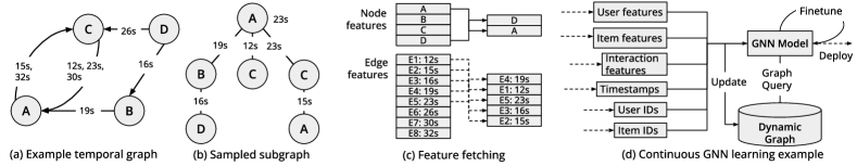
Figure 1. Figure (a) shows a temporal graph where edges are associated with timestamps. Figure (b) displays the result of temporal 2-hop sampling on node A at timestamp 23s, resulting in a subgraph. Figure (c) shows feature fetching for the subgraph in Figure (b). Figure (d) shows a concrete example of continuous GNN learning.

Further, feature fetching of dense node and edge features presents new challenges in continuous learning over dynamic graphs. Previous GNN systems proposed static GPU-based feature caches to reduce the transmission of node features, which requires careful cache initialization before training. For instance, PaGraph (Lin et al., 2020) caches features of nodes with the highest node degrees, while GNNLab proposes a presampling method (Yang et al., 2022b), which samples the graph for several epochs and caches the features of the most visited nodes. These approaches work well in offline training scenarios involving tens of epochs using all data. However, in continuous learning, the cache needs to be re-initialized before each round, which brings two major issues: 1) the limited number of epochs trained in each round (typically 2-3 to avoid overfitting on new data (Perini et al., 2022)) makes it challenging to amortize the cache initialization time (Figure 14(b)); and 2) a substantial amount of features to be cached are already stored in the cache, making it unnecessary to perform costly cache initialization in each round (§2.2). Moreover, previous works only focus on caching node features, but overlook the importance of caching edge features. Edge features are widely used in temporal GNN models to capture temporal dynamics (da Xu et al., 2020; Rossi et al., 2021). We discover that approximately 62.2% to 99.3% of the total feature communication is dedicated to transferring edge features for dense graphs (§2.2). We further find that when training temporal GNNs on dynamic graphs, the access to edge features follows an exponential distribution with a notable degree of access to numerous edge features (§4.3). This makes previous static cache designs ineffective for edge features, highlighting the need for dynamic caching of features.

To address these challenges, we develop GNNFlow, a distributed deep graph learning framework for efficient continuous GNN training over dynamic graphs on multi-GPU machines. The main contributions of GNNFlow are summarized as follows.

$\triangleright$ We propose an efficient time-indexed block-based data structure for storing dynamic graphs (§4.1). It uses adaptive block size to balance memory usage and the efficiency of graph updates and sampling operations.

$\triangleright$ We propose a hybrid GPU-CPU graph data placement for fast GPU-based temporal neighborhood sampling by storing frequently accessed lightweight graph metadata on the GPU and heavy graph edge data on the host shared memory (§4.2). We also make kernel optimizations to improve the sampling process.

$\triangleright$ We develop a dynamic GPU cache for both node and edge features, improving the cache hit rate with cache reuse and restoration (§4.3). We also introduce a vectorized cache design for batch updates to boost efficiency.

$\triangleright$ We support distributed training by partitioning graphs (topology and features) on multiple machines (§4.4). We propose static scheduling for distributed sampling to ensure load balance.

$\triangleright$ We implement GNNFlow using DGL (Wang et al., 2019) and PyTorch (Paszke et al., 2019), and compare its performance with TGL (Zhou et al., 2022) and DGL. Note that while GNNFlow is designed for continuous temporal GNN learning on dynamic graphs, it also supports static GNN models like GCN (Kipf and Welling, 2017), GraphSAGE (Hamilton et al., 2017), and GAT (Veličković et al., 2018), as well as training on static graphs. Our evaluations demonstrate that GNNFlow enables up to 21.1x speed-up compared to TGL in continuous learning of temporal GNN models (including TGN (Rossi et al., 2021), TGAT (da Xu et al., 2020), and DySAT (Sankar et al., 2020)) on large real-world graphs with 8 GPUs. Additionally, we achieve up to 1.46x higher training throughput when training GraphSAGE (Hamilton et al., 2017) and GAT (Veličković et al., 2018) on a large partitioned static graph on 4 Amazon EC2 g4dn.metal instances, compared to distributed DGL. Notably, GNNFlow can efficiently train temporal GNNs on a dynamic graph with 5 billion edges on 8 g4dn.metal instances, while other systems cannot support this scale.

2. Background and Motivation

2.1. GNN Learning on Dynamic Graphs

Dynamic graphs. There are two main models of dynamic graphs: Discrete-time dynamic graphs (DTDG) and continuous-time dynamic graphs (CTDG). DTDGs are sequences of static graph snapshots taken at regular intervals. CTDGs are represented by lists of timestamped events, such as edge and node additions or deletions. We focus on CTDGs for two main reasons. First, CTDGs offer a more flexible and detailed representation of dynamic graphs compared to DTDGs, capturing graph evolution at the event level. Second, many recently proposed temporal GNN models are designed specifically for CTDGs, which outperform DTDG-based ones on tasks like node classification and link prediction (da Xu et al., 2020; Rossi et al., 2021).

Temporal graph neural networks. Traditional GNN models for static graphs like GCN (Kipf and Welling, 2017) and GAT (Vaswani et al., 2017) employ a message-passing paradigm  (Gilmer et al., 2017) to propagate node information to neighbors and compute node embeddings by aggregating neighborhood information. Temporal GNNs are designed for temporal graphs, which adopt message passing and temporal neighborhood sampling for embedding generation. Models like TGN (Rossi et al., 2021) and TGAT (da Xu et al., 2020) use temporal graph attention, with TGN also using a node memory module (a software module different from device memory). DySAT (Sankar et al., 2020), designed for DTDGs, can also be extended to CTDGs (Zhou et al., 2022).

Temporal GNNs training. The training (or target) nodes are divided into mini-batches and iteratively trained, with one mini-batch processed in one training iteration. Temporal GNN training processes the dataset in strict time order (Zhou et al., 2022). Each training iteration can be divided into three phases: temporal k-hop sampling, feature fetching, and model training.

Temporal k-hop sampling involves selecting a subset of the node $v$’s neighbors based on a specific timestamp $t$ (da Xu et al., 2020). The edges connecting these neighbors must have timestamps that fall within a given time range of $[t-\delta,t]$. Temporal multi-hop sampling is a recursive process that samples each hop, resulting in a tree (subgraph) with node $v$ at its root. Figure 1 (b) shows a toy example. Note that in the first hop, node C is sampled twice because there are two edges (12s, 23s) that meet the condition. TGN uses recent sampling to select a given number of neighbors closest to the given timestamp $t$, while TGAT uses uniform sampling, which randomly selects a subset of neighbors from all candidate neighbors. DySAT uses a specified time window for $\delta$. Static GNN models like GraphSAGE (Hamilton et al., 2017) and GAT (Vaswani et al., 2017) can also adapt to temporal neighbor sampling, which is similar to the uniform sampling used in TGAT. After obtaining a sampled subgraph, we need to fetch the features of the sampled nodes/edges from disk/CPU memory, and copy them to GPUs for GNN computation. Figure 1 (c) provides an example. Only the features of the outermost sampled nodes (i.e., nodes D and A) and all sampled edges in the subgraph are required.

In distributed GNN training, a large graph is partitioned among multiple machines, and each GPU/machine processes a subset of the training nodes using data-parallel training (Liu et al., 2023). During each phase of a training iteration, communication is necessary for data exchange among the machines (Zheng et al., 2020). Neighbor information of training nodes not in the local graph partition must be transferred for neighborhood sampling. During feature fetching, machines retrieve node/edge features and node memories from others for those not in the local graph. In GNN computation, the machines synchronize gradients among each other for model parameter updates.

Continuous GNN learning on dynamic graphs. Figure 1 (d) illustrates a concrete example of continuous learning in the context of a real-time recommendation system scenario, such as short video recommendation (Lin et al., 2022). In this scenario, new user/item interaction events are constantly generated, with both users and items having features, and the interactions themselves also having features (e.g., viewing duration, number of likes, comments, etc.). These generated events are batched (e.g., every hour) and simultaneously update the live dynamic graph and are used to finetune the GNN model on GPU machines. The finetuned GNN model can then be deployed immediately, allowing for continuous improvement and adaptation to changing user preferences and item attributes. While finetuning a GNN with new data can improve adaptation to changing patterns, it risks catastrophic forgetting of previously learned knowledge. Experience replay addresses this by incorporating both new and historical data when finetuning to mitigate catastrophic forgetting (Perini et al., 2022).

Table 1. Qualitative comparisons of different systems.

System	Dist.	Temp. Neighb.	GPU	GPU Feature
	CTDGs	Sampling	Sampling	Cache
DGL (Wang et al., 2019)			✓
TGL (Zhou et al., 2022)		✓
GNNLab (Yang et al., 2022b)			✓	✓
PlatoGL (Lin et al., 2022)	✓
GNNFlow	✓	✓	✓	✓

Table 2. Overhead of building and partitioning large graphs.

Framework	Load and Build	Partition	Training
TGL (Zhou et al., 2022)	0.5 hr	N/A	2.5 hr
DGL (Zheng et al., 2020)	0.7 hr	2.7 hr	5.2 hr

2.2. Limitations of Existing Systems & Challenges

Table 1 shows a qualitative comparison among existing systems. DGL (Wang et al., 2019), a widely used GNN framework, assumes static graphs and supports distributed GNN training over multiple machines (Zheng et al., 2020). TGL (Zhou et al., 2022) trains temporal GNNs on pre-stored static temporal graphs on a single multi-GPU machine. Its following work DistTGL (Zhou et al., 2023) focuses on memory-based temporal GNNs but still assumes a static graph storage and does not partition graphs in distributed training. GNNLab (Yang et al., 2022b) focuses on training static GNNs on static graphs with a GPU-based sampler and static feature cache. PlatoGL (Lin et al., 2022), though it supports continuous learning over distributed CTDGs, does not support temporal GNNs. Furthermore, it is not open-source, and thus we are unable to perform quantitative comparisons.

Limitation 1: Large overhead to build and partition large static graph snapshots. We examine the overhead of graph reconstruction in training TGN using TGL and GraphSAGE using DGL on AWS g4dn.metal instances using the MAG dataset (Zhou et al., 2022). TGL’s graph construction was rewritten in C++ with multi-threading for efficiency. TGL does not support distributed training on partitioned graphs. Thus, its partition time has not been demonstrated. As shown in Table 2, despite the improvements, graph construction and partitioning can take 30 minutes to several hours, making up 20% to 65% of training time in an epoch. This significant overhead limits the training frequency for both TGL and DGL on updated data.

Challenge 1: Design an efficient CTDGs storage that efficiently supports temporal k-hop sampling. Choosing the right data structure for CTDGs that supports graph updates and temporal neighborhood sampling without excess memory use is critical. While an adjacency list is a simple choice, querying neighbors requires traversing the whole lists, which is inefficient with long lists. Block-based adjacency lists can help by dividing neighbors into blocks, but the block size needs careful selection to balance efficiency and memory use. Previous dynamic graph processing systems like Tegra (Iyer et al., 2021) inefficiently handle fine-grained temporal queries, treating dynamic graphs as snapshot sequences. Temporal k-hop sampling in this approach would create millions of snapshots for large graphs, equal to the number of edges. In Aspen (Dhulipala et al., 2019), a graph is represented as tree-of-trees: a purely-functional tree stores the set of vertices (vertex-tree), and each vertex stores the edges in its own C-tree (edge-tree). However, it does not support temporal k-hop sampling, and its tree structure is not optimized for GPU operations. To address this challenge, we propose a time-indexed block-based adjacency list with adaptive block size to address the challenge (§4.1).

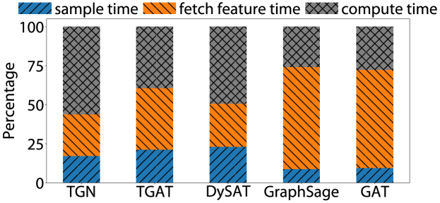
Figure 2. GNN training time breakdown for TGL and DGL.

Limitation 2: Inefficient graph queries becoming the main bottleneck of GNN training on dynamic graphs. Existing systems, like DGL and TGL, are not well-optimized for neighborhood sampling and feature fetching in dynamic graphs. They use CPUs for sampling and require copying features from CPU to GPU. Later releases of DGL utilize unified virtual addressing (UVA) for sampling. We run TGL to train three temporal GNNs (TGN, TGAT, DySAT) and DGL to train GraphSAGE and GAT with graph partition on the GDELT graph (Zhou et al., 2022). Figure 2 shows that neighborhood sampling and feature fetching account for 43% to 73% of total training time, creating bottlenecks in model learning. Inefficient graph queries also limit retraining frequency. Some studies propose GPU-based sampling and feature cache (Lin et al., 2020; Yang et al., 2022b; qui, 2022) for static graphs, but they do not address dynamic graphs.

Challenge 2: Efficiently use GPUs to accelerate temporal neighborhood sampling on dynamic graph. Due to the limited memory capacity of GPUs, previous works have proposed hosting the graph in pinned host memory and using unified virtual addressing (UVA) to access necessary graph data for large static graphs (qui, 2022; Sun et al., 2023). However, for dynamic graphs, this method would incur substantial CPU-to-GPU data copying overheads during temporal neighborhood sampling. This is because dynamic graphs typically utilize a pointer-based data structure, leading to scattered graph data. Therefore, finding neighbors requires pointer-chasing, where each memory access inevitably results in a CPU-to-GPU data copy. Moreover, in a distributed multi-GPU setting, achieving load balancing among GPUs when performing sampling poses a challenge. To address this challenge, we propose an efficient GPU-based temporal neighborhood sampling design for distributed GNN training, which places frequently accessed graph metadata on GPUs, employs several kernel optimizations, and evenly distributes the sampling workload among workers (§4.2).

Table 3. The percentage of edge feature transmission in the total feature transmission.

Model	Reddit (Kumar et al., 2019)	GDELT (Zhou et al., 2022)	Netflix (Bennett et al., 2007)
TGN	82.2%	72.4%	26.9%
TGAT	88.6%	99.3%	35.9%
DySAT	62.2%	89.2%	28.0%

Limitation 3: Ineffective feature caching in existing GPU-based designs for dynamic graph learning. Previous works on GPU feature cache focus on static cache, requiring careful cache initialization to cache features of frequently accessed nodes. PaGraph (Lin et al., 2020) uses a node-degree-based method. GNNLab  (Yang et al., 2022b) proposes a presampling method, which samples the graph for several epochs and caches the features of the most visited nodes. However, The initialization time for the cache may account for up to 90% of its feature fetching time (including cache initialization) (Figure 14(b)). Furthermore, we have also found that nearly 92% of node features and 22% of edge features to cache are actually already on the cache (Table 4). This indicates that it is unnecessary to perform the expensive cache initialization every time retraining is carried out. Moreover, most existing studies focus on static caching of node features, overlooking edge feature caching (Rossi et al., 2021; Zhou et al., 2022). Table 3 shows that, for dense Reddit and GDELT graphs, edge feature communication accounts for 66.2% to 99.3% of total feature communication (including TGN’s node memory communication). For the sparse Netflix graph, this percentage is lower due to its large node count and high node feature dimension (768). Therefore, a new cache design is required to optimize GPU feature caching for continuous learning on dynamic graphs.

Challenge 3: Optimize GPU feature cache for continuous learning. We discover that node feature access patterns follow a power-law distribution, allowing us to cache only a small portion of frequently accessed nodes (Figure 5). In contrast, edge feature access patterns follow an exponential distribution, resulting in a significant degree of access to many edge features, rendering the aforementioned approach ineffective. To address this challenge, we propose using a vectorized dynamic cache with cache reuse and restoration to address the challenge (§4.3).

3. Overview

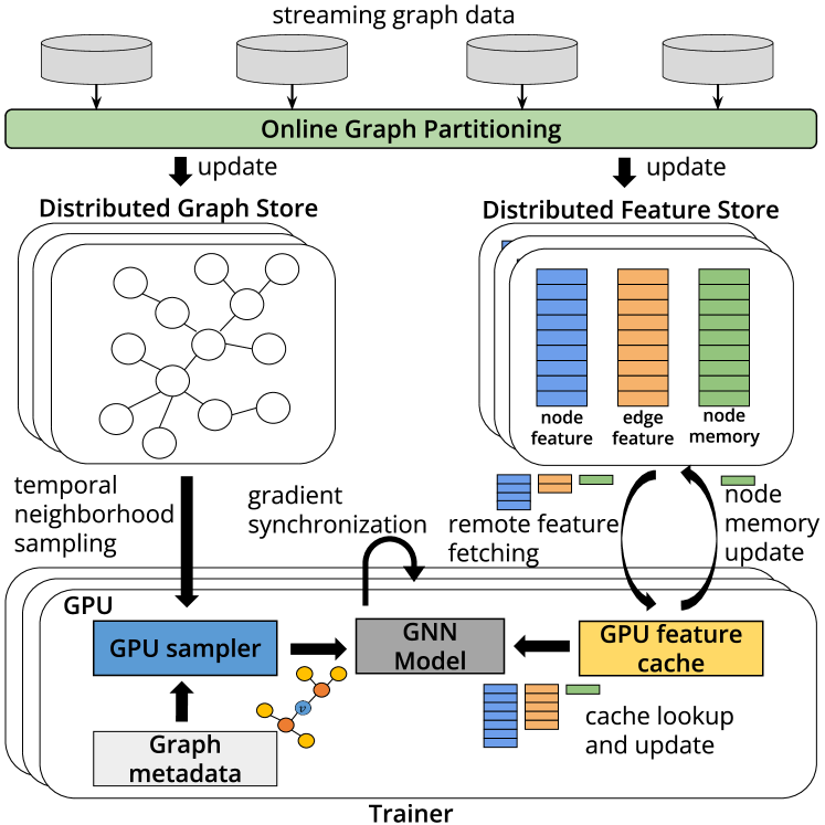
Figure 3. Architecture of GNNFlow

We design GNNFlow, a distributed graph learning framework tailored for continuous temporal GNN training on dynamic graphs. It also supports static GNN models and offline training on static graphs. We consider a dynamic graph $\mathcal{G}(t)$ that constantly receives updates (i.e., node and edge insertion and deletion) over time. Our system obtains a GNN model $M(t)$ that learns up-to-date information from $\mathcal{G}(t)$.

Figure 3 illustrates the architecture of GNNFlow, comprising a distributed graph store, a distributed feature store (both in host memory), and a trainer (sampler and feature cache) on each GPU. The system processes streaming graph updates in incremental batches, following common practice in dynamic graph processing systems (Ediger et al., 2012). New graph data (nodes, edges, features) received between $t$ and $t+1$ are batched into incremental batch $\mathcal{G}(t,t+1)$. Upon batch arrival, the system dispatches new data to machines using an online partitioning method (4.4) and stores graph structure data and features in respective stores. Model retraining (aka finetuning) is triggered, where the current GNN model $M(t)$ is finetuned with new data $\mathcal{G}(t,t+1)$ and possibly historical data.

Iterative mini-batch training is adopted for model retraining upon each incremental batch, using GPUs on multiple machines. In each training iteration, a trainer queries the distributed graph store for temporal neighborhood sampling (§4.2). Then the trainer fetches node/edge features of the sampled subgraphs: it looks up its GPU feature cache and invokes the feature fetching service to retrieve features not in the cache. The feature cache is updated dynamically (§4.3). Afterward, the trainers perform GNN computation, including forward computation, backward computation, and gradient synchronization. Finally, if node memories are used, the updated memory is written back to the distributed feature store. The dynamic graph storage is not updated during this retraining process; the incoming data received during this time are buffered as the next batch.

4. System Design

4.1. In-memory Dynamic Graph Storage

We propose block-based neighborhood storage, allowing efficient updates and queries in dynamic graph learning, as illustrated in Figure 4. This data structure exploits temporal locality to enable fast insertion of new nodes/edges and efficient temporal neighborhood sampling (§4.2). It consists of a node table and a list of edge blocks for each node.

The node table is a contiguous array, with each entry corresponding to one node and a doubly-linked list of edge blocks that store all edges connected to that node. Each node entry contains pointers to the first and last edge blocks in the node’s doubly-linked list, the number of edge blocks (list length), the total number of edges connected to the node (node degree in an undirected graph and out-degree in a directed graph) and a validity field indicating whether the node still exists. Adding a node is achieved by simply appending an entry to the table. Node deletion is indicated by setting the validity field of the node to 0.

The edge blocks are lightweight structures (72 bytes), each storing graph metadata about a group of edges, including the block size (maximal number of edges that can be contained in the block), the actual number of edges in the block, pointers to the graph edge data, and the earliest and latest timestamps of edges in the block. The graph edge data are lists of neighbor IDs, edge IDs, edge timestamps, and validity indicators. The same entry in the lists corresponds to one edge in the edge block: the respective neighbor ID is the ID of the neighbor to which the edge is connected, edge ID is the ID of the edge, the timestamp is when the edge is inserted, and the validity indicates if the edge is present or deleted. The lists are organized in increasing order of edge timestamps.

Edge blocks at each node are chronologically ordered, with the oldest edges in the edge block at the list head and the newest edges in the edge block at the tail. Chronologically ordering edge blocks and edges in each edge block brings two main advantages. (1) It enables efficient temporal queries, such as finding all edges within a given time range, by sequentially scanning only a subset of the edge blocks rather than the entire list (§4.2). Within each block, logarithmic-time neighborhood search is allowed over the sorted edges. (2) It enables efficient edge insertion: new edges can be appended to the tail of an existing edge block when the last block still has capacity, or added into a new block to be linked to the tail of the edge block list, without requiring costly re-sorting.

For node/edge deletions, we mark the corresponding validity fields while preserving data layouts and pointers. Invalid nodes/edges are ignored during sampling.

In dynamic graph storage, continuous data addition may cause out-of-memory errors, while old data may no longer be relevant for training. We provide an API that can offload data older than a specified timestamp to a file.

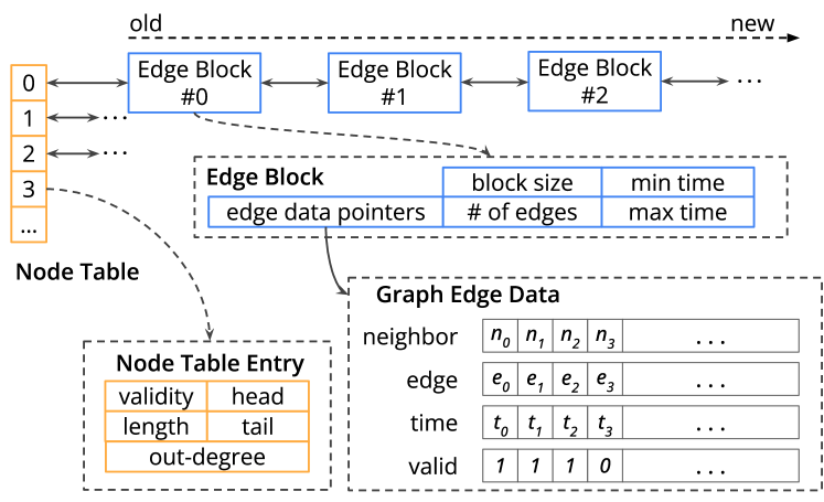
Figure 4. Block-based neighborhood storage

Adaptive block sizing with threshold. The edge block size in our dynamic graph data structure is a critical hyperparameter, balancing memory usage and graph operation efficiency. Small block sizes increase memory consumption and overhead due to more edge blocks per node and costly temporal neighborhood sampling as there are more blocks to traverse. Conversely, large block sizes lead to space wastage due to less densely filled edge blocks.

We adopt adaptive block sizing for each node that adapts to the changing graph over time. Many real-world graphs follow a power-law degree distribution, with most nodes having only a few neighbors and a small set of nodes densely connected (Faloutsos et al., 1999). We set a threshold of node out-degree (decided using grid search in §6.2): when the out-degree of a node is smaller than the threshold, the edge block size of the node is set to its out-degree; otherwise, the block size is set to the threshold. Therefore, the size of the allocated block for a node $v$ , denoted as $b_{v}$, is determined by $b_{v}=\min(deg(v),\tau)$, where $\tau$ is the threshold and $deg(v)$ is the node $v$’s current degree. For the majority of nodes whose neighbor numbers are small, setting an edge block size equivalent to the out-degree significantly reduces the length of the block list, and a new block’s addition (with space reserved for future neighbors) does not incur excessive space overhead. For nodes with many neighbors, adding a new block with a large block size may result in significant memory waste (when the new block is sparsely filled), and hence we limit its block size by the threshold. The upper bound of wasted space (i.e., not filled by edges) is less than half of the total number of edges in the graph. By adaptively adjusting the block size based on each node’s out-degree, we balance memory consumption and graph update/query efficiency. Note that the block size change applies only to new blocks to be appended, and the sizes of existing edge blocks remain unchanged.

4.2. GPU-based Graph Sampling

Algorithm 1 shows the process of temporal neighborhood sampling on GPUs. Given a batch of target nodes and their time ranges, the algorithm traverses through each target node’s linked list in parallel, skipping any edge blocks that do not coincide within the given time range. Within each edge block, if the minimum to maximum timestamps overlap with the specified time range, the algorithm employs a binary search on the candidate neighbors. Subsequently, a predetermined number of these candidate neighbors are selected through a sampling method, such as recent sampling or uniform sampling (§2.1). For multi-hop neighborhood sampling, the process is repeated for each GNN layer, using the sampled nodes from one layer as the input to the next-layer sampling (Zhou et al., 2022). Note that the system can also efficiently support other sampling methods. For example, we can support temporal random walk (Nguyen et al., 2018) by setting the neighborhood sample size of each layer to one (Pandey et al., 2020).

Algorithm 1 Temporal Neighborhood Sampling

1:Input: block-based graph storage (node table $V$), target nodes $\mathbf{n}$, start timestamps $\mathbf{t_{s}}$, end timestamps $\mathbf{t_{e}}$, neighborhood sample size $f$

2:Output: temporal neighbors for each $n\in\mathbf{n}$

3:parallel for $n\in\mathbf{n}$, $t_{s}\in\mathbf{t_{s}}$, $t_{e}\in\mathbf{t_{e}}$ do

4:      $\text{candidates}=[]$

5:      $lst=V[n]$

6:      $b=lst.tail$ // the newest block

7:      while $b\neq null$ do

8:           if $t_{e}<b.t_{\text{min}}$: $b=b.prev$  continue

9:           if $t_{s}>b.t_{\text{max}}$: break

10:           find neighbors within time window $[t_{s},t_{e})$ using binary search in $b$ and add them to candidates

11:           $b=b.prev$

12:     end while

13:     sample $f$ neighbors from candidates

14:end for

Hybrid GPU-CPU graph data placement. Due to the limited memory capacity of GPUs, the graph data are commonly stored in host memory. Substantial data copying overheads from CPU to GPU are incurred during GNN training, especially on dynamic graphs, which requires frequent access to graph data. For instance, during temporal neighborhood sampling (Algorithm 1), several edge blocks are accessed, followed by retrieving the graph edge data referenced by these edge blocks. Previous works have proposed hosting the graph in pinned host memory and using unified virtual addressing (UVA) to access necessary graph data (qui, 2022), which still requires frequent CPU-to-GPU copies.

We note that graph metadata (i.e., node table and edge blocks) is accessed more frequently than graph edge data: the former is first accessed before the latter are retrieved, and many edge data are skipped during neighborhood sampling (e.g., because they are not in the specified time range) while their metadata is accessed. We leverage the fact that graph metadata is usually several orders of magnitude smaller in size than the graph edge data (Table 6) and store graph metadata in global memory on GPUs to reduce frequent CPU-to-GPU copies, while placing the large graph edge data in host memory (Graph Store in Figure 3). In this way, we can significantly accelerate GPU-based graph queries (§4.2).

On a multi-GPU machine, the graph edge data is shared among trainers through page-locked host memory mapped into the CUDA address space of each GPU, allowing direct access by any GPU across the PCIe bus. The trainer of rank 0 is responsible for updating the graph storage over time, while all trainers can query the graph data. By mapping page-locked host memory into CUDA, the edge data appears in local GPU memory for high-bandwidth, low-latency concurrent read accesses by multiple GPUs, while atomic updates from rank 0 are instantly propagated.

Kernel optimizations. We initiate a GPU thread to sample one neighbor of a given target node following previous works (Yang et al., 2022a; Jangda et al., 2021). We sample neighbors of the same target node by adjacent threads, which helps to reduce warp divergence by minimizing the differences in the operations performed by each thread. We also ensure sampled results written to global GPU memory are consecutive to support coalesced access. To reduce GPU global memory access during sampling, each thread caches its currently accessed lightweight edge block (72 bytes) in its registers. For uniform sampling, we record candidate neighbors’ positions in edge data lists before selection in GPU’s shared memory to reduce GPU global memory access. With recent sampling, we directly select the latest candidates.

4.3. Feature Cache on GPUs

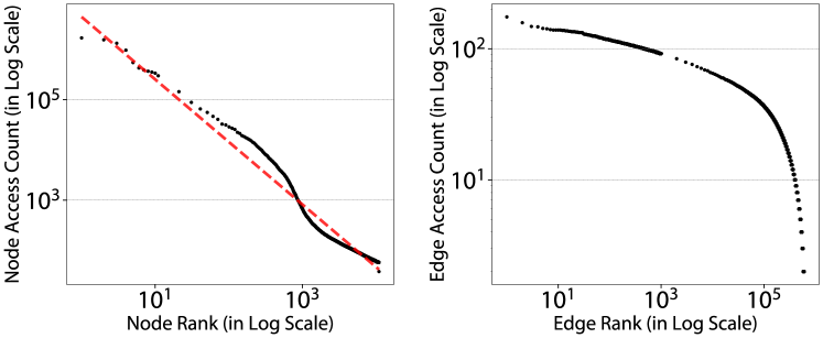
Figure 5. Distributions of node and edge accesses when training TGAT on Reddit. Red dashed line denotes linear fitting.

Table 4. Jaccard similarity of the set of all sampled nodes/edges in adjacent retraining rounds of TGAT model.

Dataset	Reddit (Kumar et al., 2019)	GDELT (Zhou et al., 2022)	Netflix (Bennett et al., 2007)
Node	99.5%	95.0%	87.5%
Edge	91.9%	27.6%	29.3%

Observation. We discover a notable amount of duplication in the nodes and edges sampled between adjacent continuous learning rounds. Table 4 displays the Jaccard similarity (Jaccard, 1912) of the sets of sampled nodes and edges for each dataset between adjacent continuous learning rounds. We observed a high similarity of 99.5% in the sets of nodes, whereas the similarity in the sets of edges was lower, possibly due to the higher number of edges compared to nodes. These results indicate that there is an opportunity for data reuse.

Moreover, we analyze node and edge access patterns when training GNNs. Figure 5 shows the distributions of node/edge access counts when training TGAT on Reddit (Rossi et al., 2021). We observe that the node access follows a power-law distribution, with a few nodes frequently retrieved and the majority of nodes accessed much less. This can be attributed to the common structure of real-world graphs, where a small number of “hub” nodes are more connected and thus more likely to be accessed during training. It also helps to explain the success of the static node feature cache adopted in PaGraph (Lin et al., 2020) (caching nodes with the highest out-degrees) and GNNLab (Yang et al., 2022b) (caching a small subset of frequently accessed nodes). However, the edge access follows an exponential distribution, with most edges accessed to some extent. This pattern makes static cache unsuitable as it cannot effectively capture the wide range of edge accesses. We observe similar node/edge access patterns when training other temporal GNNs (e.g., TGN) on other datasets (including Wikipedia (Rossi et al., 2021), MOOC (Kumar et al., 2019), LastFM (Kumar et al., 2019) and GDELT). When training GNN models for static graphs (e.g., GraphSAGE), the edge access obeys a skewed distribution.

Based on these observations, we advocate utilizing GPU-based dynamic feature caching (such as LRU (O’neil et al., 1993), LFU (Matani et al., 2021), FIFO) for continuous learning, and fully exploiting data reuse through inter-round cache reuse and intra-round cache restoration.

Cache reuse and restoration. First, we exploit the inter-round feature fetching duplication (Table 4) by recording the cache contents (e.g., to disk) at the end of each round and loading the cache into GPU memory at the beginning of the next round. This reuse avoids high cache miss rates caused by cold cache startups and avoids long cache initialization times caused by static cache methods. Second, a retraining round typically requires multiple epochs to converge, and each epoch traverses the training samples in strictly temporal order (§2.1). However, at the beginning of the second epoch, the dynamic cache has already been replaced with newer node/edge features, which can be considered “polluted”, resulting in a large number of cache misses. To counter this, we save the cache contents (for example, to CPU memory) at the start of each round, and restore the cache at the beginning of every epoch. This technique improves the cache hit rate at the start of each new epoch.

Vectorized cache. In each training iteration, feature fetching often requires accessing features of thousands of nodes and edges, with no particular order among them. Typical dynamic cache implementation is inherently inefficient, not able to handle batched accesses in parallel. For example, LRU cache usually assumes a single access at a time, updating cache entries one by one (O’neil et al., 1993). The standard doubly-linked list structure and locking mechanism required for thread safety in LRU cache may severely hinder efficiency (Fan et al., 2013).

We design a highly efficient vectorized cache that enables parallel access and update of cache entries in batches. For example, in our vectorized LRU Cache, we store a “recent score” for each cache entry in a vector. The scores represent how recently each entry was last accessed, with 0 meaning most recently. Initially, all recent scores are 0. Upon each update, all recent scores are decremented by 1. An access resets the corresponding entry’s recent score to 0. For replacement, the entries with the lowest recent scores are evicted using an efficient vectorized top-k operation. For vectorized LFU cache, we adopt a similar approach by changing the recent score to an access count. The vectorized FIFO cache is implemented using a ring buffer, which maintains a pointer to the most recently cached node or edge features. During each batch update, the pointer only needs to be moved by the number of entries that are to be replaced in the ring buffer.

In addition, sometimes a large number of items need to be replaced in a dynamic cache (e.g., LRU), resulting in most or even all cache items being replaced. This could potentially lead to cache thrashing, where items are frequently replaced. We limit each cache update to at most a fraction $\lambda$ of its capacity ($0<\lambda<=1$). This strategy can help maintain the stability of the cache, avoid frequent replacement of cache items, and thus maintain a higher cache hit rate. In subsequent experiments, we set $\lambda=0.2$ by default.

4.4. Distributed Training on Partitioned Graphs

Distributed storage. When graph data exceeds a single machine’s RAM capacity, partitioning is needed. We use the edge-cut model (Malewicz et al., 2010; Low et al., 2014), storing each node and its associated edges and features on one machine. Edge-cut is favored over vertex-cut (Xie et al., 2014; Petroni et al., 2015), as it reduces cross-machine communication while vertex-cut distributes node neighbors to multiple machines and causes high latency for sampling due to multi-machine access. Existing edge-cut partitioning methods, such as the widely used METIS (Karypis and Kumar, 1998), are primarily designed for static graphs and not suitable for dynamic graphs due to high re-computation cost (§2.2). Some online partitioning methods (e.g., Fennel (Tsourakakis et al., 2014)) aim at node balance but not edge balance among the partitions. Achieving edge balance is important, to balance computation and communication workloads in distributed GNN training. We utilize a simple yet effective online hash partitioning method that assigns each node to a partition (machine) of index ${hash}({n})\%P$, where $n$ is the node ID and $P$ is the number of machines. We use an identity hash (i.e., $hash(x)=x$) due to computation simplicity and that it evenly distributes nodes and their associated edges across the machines (Gandhi and Iyer, 2021). Since node IDs and their connectivity are typically randomly distributed across the graph, this leads to more edge-balanced partitions (Barabási and Albert, 1999).

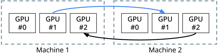
Figure 6. Static scheduling of distributed sampling

Distributed sampling. To ensure balanced workloads among trainers, we may need to assign some trainers to nodes outside their local graph partition. In these cases, we use remote neighborhood sampling on machines that store the relevant nodes. When a trainer needs to perform multi-hop sampling beyond the local machine, remote sampling is needed. To manage these requests, we propose a static scheduling approach (shown in Figure 6) that assigns GPUs on a machine to handle remote sampling requests from trainers. When a trainer needs to sample a remote target node, they send an RPC request to the machine that stores the node, targeting the GPU with the same rank as the trainer’s local GPU. We empirically validate the effectiveness of this approach by measuring the average coefficient of variance (CV) of sampling times for temporal and static GNN models (TGN, TGAT, DySAT, GraphSAGE, and GAT) on the GDELT graph using four AWS g4dn.metal instances. The CVs are very low (less than 0.06), indicating a good load balance.

Distributed feature store. Inside each machine, node/edge features and node memories are stored in shared host memory for all trainers to share. We store node features and memories using a key-value map (Python dictionary) mapping node IDs to feature vectors. New edges have larger IDs, and edge features are stored in ascending order. This enables efficient edge feature queries using PyTorch’s optimized binary search function searchsorted.

5. Implementation

We implemented GNNFlow in 8,400 lines of code (LoC) in C++ and Python. The dynamic graph storage data structure was implemented in 2,000 LoC of C++. GNN models, GPU feature cache, and distributed module (including online graph partitioning, distributed sampling, and remote feature fetching) were implemented in 5,000 LoC of Python. We also implemented CUDA kernels for temporal neighborhood sampling using 400 LoC of CUDA. We implement various static and temporal GNN models on DGL 0.9.1 with PyTorch 1.13 as the underlying deep learning framework. We rely on PyTorch’s RPC module (Li et al., 2020) with the TensorPipe backend (ten, 2022) to implement the distributed module, and use NCCL and Gloo for AllReduce operations of model gradient synchronization.

User interface. We provide easy-to-use Python APIs for developers. Figure 7 shows how developers can create and use dynamic graphs, temporal neighborhood samplers, and feature caches for training.

import gnnflow as gfdef train_step(model, edges, dgraph, sampler, cache):  # neighborhood sampling  mfgs = sampler.sample(edges)  # fetch node/edge features with cache  cache.fetch_features(mfgs)  # GNN training  output = model(mfgs)  ...dgraph = gf.DynamicGraph()model = gf.models.TGN()sampler = gf.TemporalKhopSampler(dgraph, fanouts=[10, 10])cache = gf.Cache(node=’LRU’, node_cache_ratio=0.01,                 edge=’LRU’, edge_cache_ratio=0.01)# update the graphnew_edges = gf.get_ingestion_batch_edges()dgraph.add_edges(new_edges)...# a typical training loopfor batch_edges in data_loader:  train_step(model, batch_edges, dgraph, sampler, cache)

Figure 7. An example to demonstrate GNNFlow’s API

Dynamic graphs. We allocate shared host memory for graph edge data storage. Each trainer registers the shared memory for use with cudaHostRegister. For adding edges in a distributed setting, there is a dispatcher that first partitions the edges according to the hash partitioning method (§4.4), and then uses PyTorch’s asynchronous RPC to call the operation of adding edges on the local partition of each trainer.

GPU-based sampling. We pre-allocate CPU pinned memory buffers and GPU buffers for input target nodes and output sampled neighbors. For each sampling layer, we invoke custom CUDA kernels, use thrust::remove_if to remove invalid neighbors, and copy results to the CPU. In static scheduling for distributed sampling (§4.2), each GPU may handle multiple requests from other machines. Thus, we use a task queue. The distributed sampler adds a sampling task to the queue, which returns a handle. The sampler polls the handle, and if the task is complete, it returns the result.

6. Evaluation

Testbed. We use Amazon EC2 g4dn.metal instances for all experiments. Each instance has 8 NVIDIA 16GB T4 GPUs, 96 vCPU cores, 384 GB memory, and 100Gbps network interconnectivity.

Datasets. We study four real-world graphs and one synthetic graph detailed in Table 5. The Reddit dataset (Kumar et al., 2019) is a bipartite graph mapping interactions between users and subreddits on Reddit. The Netflix dataset (Bennett et al., 2007) is a bipartite network connecting users and movies, with edge weights indicating rating scores from the 2006 Netflix Prize competition. The GDELT dataset (Zhou et al., 2022) is a dynamic graph documenting global events from news articles, with nodes for actors and temporal edges for events. The MAG dataset (Zhou et al., 2022) is a citation network with temporal edges and node features. The LDBC Social Network Benchmark dataset (Angles et al., 2020) is a large synthetic graph which is a list of events of members joining forums.

Table 5. Graph datasets. $|d_{v}|$ and $|d_{e}|$ are dimensions of node features and edge features, respectively. $t_{\text{span}}$ is the total time span of the temporal dataset, and $t_{\text{interval}}$ indicates the minimum time granularity recorded in the dataset.

Dataset	$|\mathbf{V}|$	$|\mathbf{E}|$	$\mathbf{d_{v}}$	$\mathbf{d_{e}}$	$\mathbf{t_{\text{span}}}$	$\mathbf{t_{\text{interval}}}$
Reddit (Kumar et al., 2019)	11K	672K	128	172	30 days	few secs.
Netflix (Bennett et al., 2007)	978K	100M	768	128	7.2 years	1 day
GDELT (Zhou et al., 2022)	17K	191M	413	186	5 years	15 mins.
MAG (Zhou et al., 2022)	122M	1.3B	768	-	10 years	1 month
LDBC (Angles et al., 2020)	113M	5.1B	-	-	3 years	few secs.

GNNs. We train three temporal GNN models (TGN, TGAT, and DySAT) and two static GNN models (GraphSAGE and GAT), using default model settings in their respective papers. The GNNs sample two layers of neighbors with 10 neighbors per layer, except for TGN, which samples one layer, and GraphSAGE, which samples 15 neighbors for the first layer.

Baselines. We compare the performance of GNNFlow with TGL (Zhou et al., 2022) (not support multi-machine training on partition graphs) and DGL (Zheng et al., 2020) (not support temporal GNNs). Note that we rewrite TGL’s graph construction code in C++ with multi-threading (128 threads) since the original Python implementation is very slow. We tune the baselines to their best configurations. As PlatoGL (Lin et al., 2022) is not open source and its implementation details are not disclosed in the paper, we are unable to conduct an end-to-end comparison of the system. Nonetheless, we compare some of its design points by implementing them in GNNFlow during the ablation study (§6.2). We also compare with various GPU-based sampling and caching baselines when evaluating individual components in GNNFlow.

Training. We perform temporal link prediction as the downstream task (i.e., predicting unseen links that will be formed in the future) in all experiments. For TGN, TGAT, and DySAT, we use a default per-GPU batch size of 4000, 600, and 600 edges, respectively. Following TGL, we use random chunk scheduling for TGN to learn inter-batch dependency in large batches. For GraphSAGE and GAT, the default per-GPU batch size is 1200. By default, we use vectorized LRU cache (§4.3) in GNNFlow, and cache 3% node features and 3‰ edge features (due to the higher number of edges) in each GPU’s memory for GDELT and Netflix, and 1% node features for MAG.

6.1. Continuous GNN Learning

Methodology. We first evaluate GNNFlow’s continuous training on dynamic graphs, comparing with TGL (with our improvement of multi-thread graph building) on 8 GPUs. We use the first 30% (in chronological order) of a dataset to train an initial model and the remaining 70% for continuous streaming updates, which are divided into incremental batches. On each new batch, we first compute the accuracy (i.e., average precision) of the current model on the new data, and then use the new data for model finetuning. We finetune the GNN model periodically (§3), finetuning the model for three epochs on new data upon each incremental batch (with an experience replay ratio of 0), in this experiment. Three epochs are the sweet point we found for balancing accuracy and training cost (Figure 10). We set the time interval $t$ for retraining to 1 day.

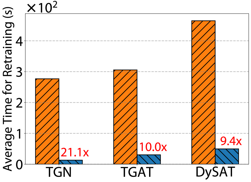
(a) GDELT

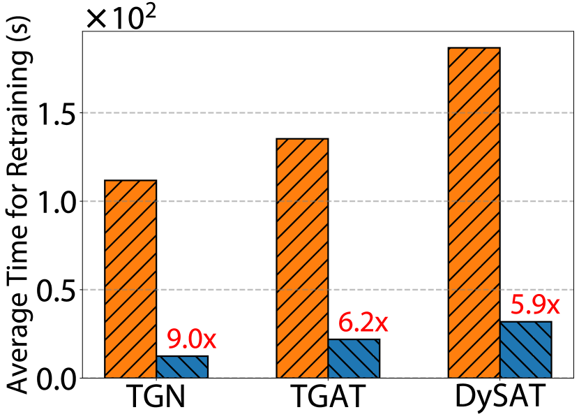
(b) Netflix

Figure 8. The average retraining time of continuous GNN learning per day for GNNFlow and TGL.

Overall performance. We measure the average total time of continuous learning upon each incremental batch (i.e., graph building/update time and model finetuning time). Figure 8 demonstrates that GNNFlow achieves 9.4x to 21.1x faster retraining than TGL on the GDELT graph and 5.9x to 9.0x speed-up on the Netflix graph. The main time consumption of TGL lies in graph reconstruction, taking on average 170.8s and 94.3s for GDELT and Netflix, respectively, accounting for up to 36.7% and 61.3% of the total time upon one day’s events. In contrast, GNNFlow only requires an average of 0.12s and 0.56s to update GDELT and Netflix graphs, with an average insertion of 96K and 130K edges. Therefore, GNNFlow can complete graph updates and training in half a minute, achieving real-time learning; whereas TGL, due to the need for graph reconstruction, requires at least several minutes for three epochs of finetuning.

Performance breakdown. Figure 9 further compares the average time taken by temporal neighborhood sampling and feature fetching during the model finetuning phase on GDELT. Our GPU-based temporal sampling (§4.2) achieves $6.3\times$ - $15.3\times$ speed-ups on the three temporal GNN models. In addition, our GPU-based vectorized LRU feature cache (§4.3) decreases the feature fetching time by up to $14.6\times$. These results validate the benefit of our GPU optimization for sampling and feature fetching.

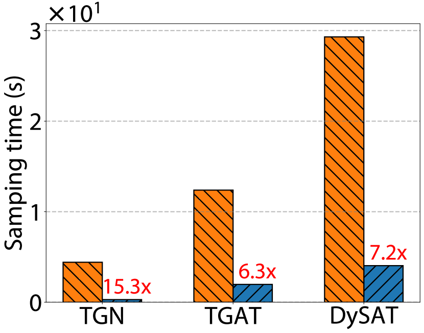
(a) Sampling speed-up

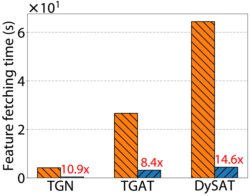
(b) Feature fetching speed-up

Figure 9. Averaged sampling and feature fetching time in continuous training on GDELT.

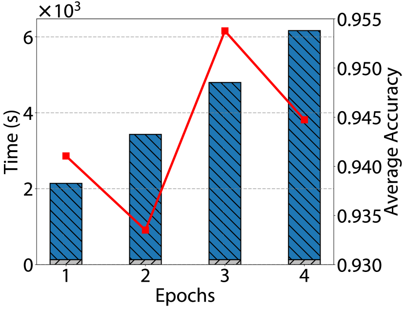
(a) TGN

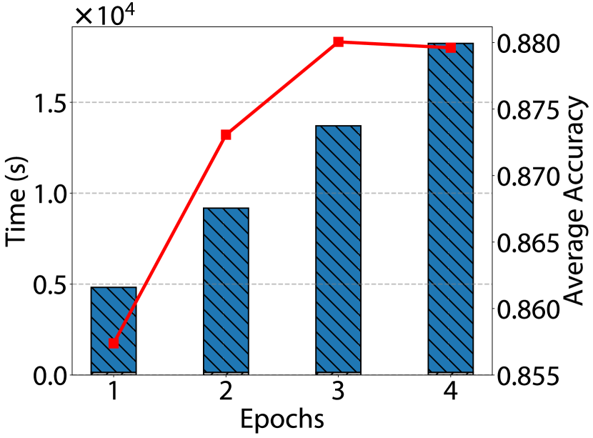
(b) TGAT

Figure 10. Impact of the number of finetuning epochs.

Impact of finetuning epoch number. We investigate the impact of the number of finetuning epochs upon each incremental batch, on model accuracy and finetuning time. We increase the finetuning epochs from 1 to 4 when continuously training TGN and TGAT on GDELT with GNNFlow. We record the average of all test accuracies on all batches and the overall time taken by updating the graph and finetuning. In Figure 10, increasing finetuning epochs results in diminishing returns on accuracy but substantial increases in finetuning time. The accuracy drops when increasing the epoch number from 3 to 4 for TGN and TGAT, potentially due to overfitting on the limited new data in each incremental batch. The results suggest that 2-3 finetuning epochs per incremental batch may strike a good balance in continuous GNN learning.

Accuracy. We further study how the retraining frequency and the experience replay ratio influence model accuracy. We observe that the total time needed for GNNFlow to finetune TGN (TGAT) for one epoch upon each incremental batch over the course of 100 incremental batches is roughly the same as that for TGL to retrain the model for one epoch once every 25 (TGN) or 50 (TGAT) incremental batches. Figure 11 shows the accuracy tested on each incoming incremental batch on the current model, when GNNFlow is retrained on each batch and TGL is retrained per 25 and 50 batches for TGN and TGAT, respectively. The percentage in the legend indicates the experience replay ratio. The ‘no retrain’ case gives the performance of the model trained using the first 30% of data, tested on each incremental batch. Being able to retrain the model more frequently within the same retraining time budget (implying the same amounts of resources), the accuracy results of TGN and TGAT trained with GNNFlow outperform those of TGL on all batches, with a gap of up to 7.2% and 9.0%, respectively. Figure 11(b) shows that a higher replay ratio results in better model accuracy because it avoids forgetting important information and thus performs well. The sudden jump in accuracy for TGL is because TGL underwent retraining at that time.

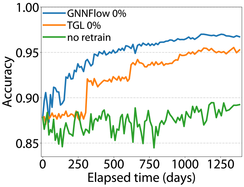
(a) TGN

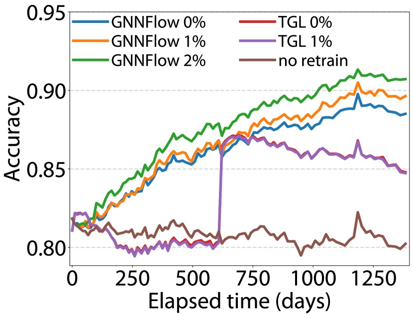
(b) TGAT

Figure 11. Model accuracy during continuous training. The elapsed time refers to the time in the GDELT dataset.

6.2. Individual Components

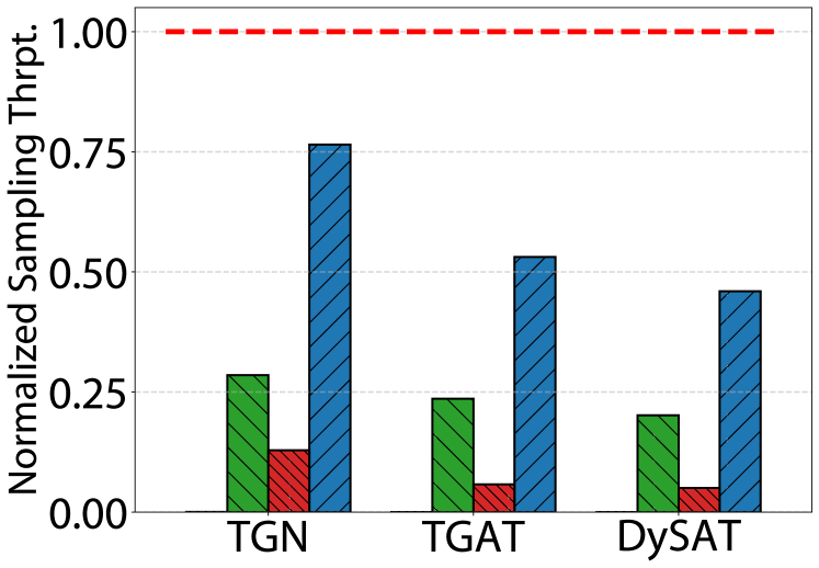
(a) GDELT

(b) Netflix

Figure 12. Normalized sampling throughput (w.r.t. static system) for different block sizing methods.

Adaptive block sizing with threshold. We compare the sampling performance of our adaptive block sizing (§4.1) against several baselines: (1) adjacency list; (2) a strawman approach, which sets a new block’s size to the number of new edges to add in each incremental batch; (3) the fixed-size approach used in PlatoGL (Lin et al., 2022), assigning each block a fixed size. We also give the results for a static system, where the complete graph is constructed all at once, resulting in an adjacency array. We use grid search to find the appropriate size/threshold for the fixed-size approach and our method, leading to a graph edge data memory overhead of around 5% (as compared to graph edge data memory usage of the static system). For GDELT and Netflix, the fixed sizes are 1024 and 48, respectively, and the thresholds in our method are 8192 and 48, respectively. In this experiment, we build each graph from scratch on one machine by injecting the graph dataset in batches with a batch size of 100,000 edges.

We observe from Table 6 that using an adjacency list can result in very long linked lists, and requires storing a large amount of graph metadata (i.e., pointers point to next or previous adjacent neighbor, etc.). Compared to the strawman approach, our adaptive block sizing reduces the final linked list length (averaged among nodes) by about 36.7x with only less than 5% more memory usage for graph edge data and reduced memory for graph metadata (due to reduced length of the linked list). With the fixed-size method, nodes with many neighbors may have very long linked lists. Our adaptive method uses larger block sizes for these nodes, which reduces their list length. Figure 12 shows that the performance of sampling using adjacency lists is extremely poor (almost 0) as nodes with many neighbors become stragglers. The fixed-size method also performs poorly compared to the strawman method for the same reason. Our method significantly improves sampling performance. The lower sampling throughput as compared to that in the static system reflects the overhead of using a dynamic graph structure.

Table 6. Linked list length and memory usage with different block sizing methods

Dataset	Method	Linked List Len.		Graph Data Size (MB)
		Avg.	Max.	Edge Data	Metadata
GDELT	Adj. List	2866.91	4.8M	3649.06	2919.25
	Strawman	233.97	1913	3649.01	238.22
	Fixed-size	12.74	18680	3843.77	12.97
	Adaptive	6.38	1896	3818.22	6.49
	Static	0.95	1	3648.69	0.96
Netflix	Adj. List	101.27	58K	3847.28	3077.83
	Strawman	32.63	984	3845.94	991.69
	Fixed-size	9.68	4854	4064.20	294.33
	Adaptive	9.04	974	4020.28	274.82
	Static	1.00	1	3833.22	30.39

(a) Reddit

(b) Netflix

Figure 13. Normalized sampling throughput (w.r.t. CPU sampling) for different sampling methods.

GPU-based sampling. We compare our GPU-based sampling with the following: (1) CPU sampling (used by TGL (Zhou et al., 2022)), with our highly optimized CPU sampler implementation for dynamic graphs; (2) CUDA-only, where all graph structure data are stored on GPU; (3) UVA-only (used by Quiver (qui, 2022) and DGL with UVA sampling feature (Wang et al., 2019)), where all graph structure data are placed on host pinned memory; and (4) unified memory (UM), which uses software interrupt and page migration with a one-page granularity for automatic migration of all graph structure data between CPU and GPU memory. We experiment on a single GPU and limit the maximum amount of GPU memory used for graph structure data to 4 GB because enough GPU memory should be reserved for GPU-based feature cache and GNN training.

As shown in Figure 13, CUDA-only and UM methods achieve the best performance on Reddit because the graph is small enough to fit entirely in GPU memory. Our method performs better than the UVA-only method as we place metadata on GPU, reducing costly copying from CPU. On the large GDELT graph, the CUDA-only method exhausts the available memory. The UVA-only method is even slower than CPU sampling because it requires frequent access to the graph metadata located on CPU. The UM method exhibits extremely poor performance due to thrashing, which is a situation that arises when GPU memory is limited and data transfers between the CPU and GPU occur frequently (Yu et al., 2020).

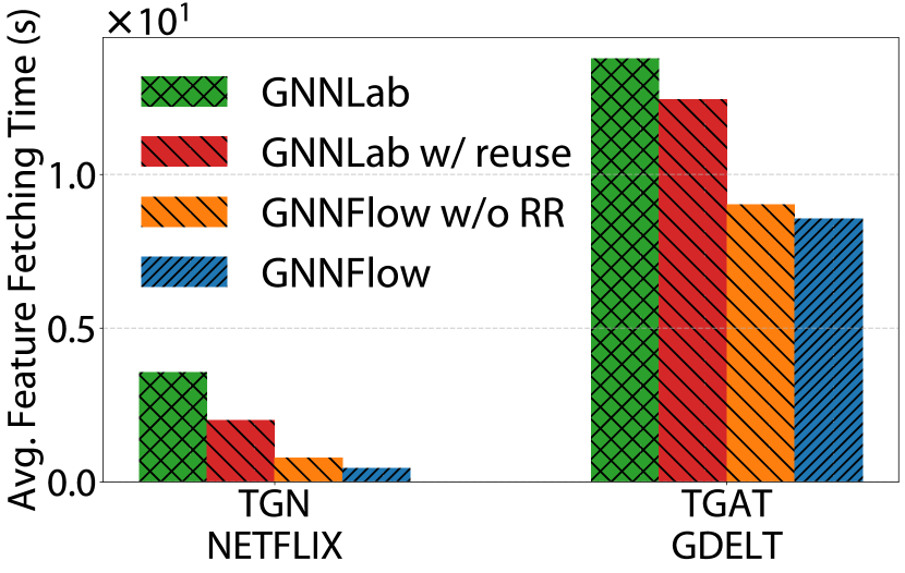
(a) Effect on different models

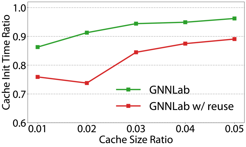
(b) Cache init. time ratio

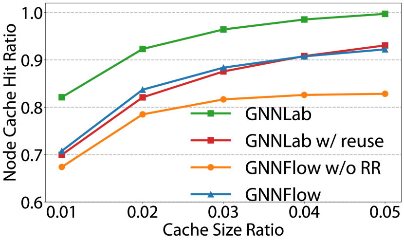
(c) Effect of node feature

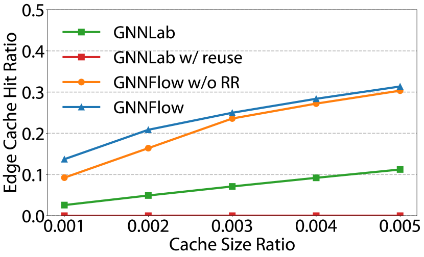
(d) Effect of edge feature

Figure 14. Performance of dynamic feature cache on diff. models and diff. cache sizes.

GPU dynamic feature cache. We compare three baselines in the same §6.1 scenario: (1) the static cache proposed by GNNLab (Yang et al., 2022b), which requires presampling with a new incremental batch for two epochs (as suggested in their paper) to re-initialize the cache in each retraining round; (2) the GNNLab static cache with cache reuse, which re-initializes the cache every two retraining rounds to allow for cache reuse between rounds; and (3) our approach without the cache reuse and restoration (noted as RR) optimizations (§4.3). We use LRU cache for all our methods, as it performs better than other dynamic cache methods on average. Figure 14(a) shows the average feature fetching time per retraining round (including cache initialization time) for continuous learning on two workloads. Our approach significantly reduces the feature fetching time by 8.1x and 1.6x compared to GNNLab in two workloads, respectively. Figure 14(b), Figure 14(c) and Figure 14(d) show the effect of cache initialization time and cache hit rate for node and features when training TGN on the Netflix graph, respectively. Figure 14(b) shows the proportion of time spent on cache initialization in GNNLab, which accounts for nearly 90% of the total feature fetching time (including cache initialization), and slightly decreases to around 80% when using cache reuse. On the other hand, our proposed vectorized dynamic cache eliminates the need for expensive cache re-initialization in every retraining round, and the cache reuse and restoration optimizations (§4.3) in GNNFlow can utilize data duplication between adjacent rounds to significantly increase the cache hit rate, as shown in Figure 14(c) and Figure 14(d), thereby reducing the feature fetching time.

In addition, Figure 14(d) illustrates the ineffectiveness of GNNLab’s static cache strategy for edge features. The cache hit rate is nearly zero without cache re-initialization in each round (GNNLab cache w/ reuse). The edges cached in previous rounds are seldom used in subsequent training. Even with cache re-initialization in each round (GNNLab), its cache hit ratio remains lower than our dynamic cache. This is because the edge access pattern is more dispersed than nodes, rendering the static cache unsuitable (S4.3).

6.3. Scalability

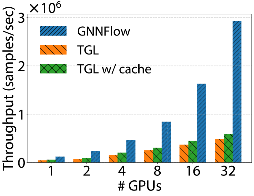
(a) TGN

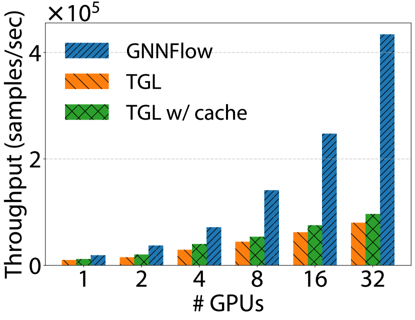
(b) TGAT

Figure 15. Training throughput with different numbers of GPUs on the GDELT graph.

We further evaluate the training throughput of GNNFlow, TGL and TGL with cache (the same LRU cache and cache ratios as GNNFlow) when training TGN and TGAT on GDELT in multi-GPU multi-machine scenarios by injecting 100 incremental batches consecutively. Since the graph (with features) can fit on a single machine, we do not partition it across multiple machines. We utilize 1 to 32 GPUs on four g4dn.metal instances. Figure 15 shows the training throughput of model retraining on the last incremental batch. GNNFlow always achieves the best training throughput while attaining near-linear scalability within a single machine and 71.9% and 76.2% of the ideal linear-scaling performance on 32 GPUs for TGN and TGAT, respectively.

Table 7. Multi-machine training of GraphSAGE and GAT on partitioned MAG graph using 32 GPUs

System	Graph Building	Model	Throughput
	Time (s)		(samples/s)
DGL	7778	GraphSAGE	124086.2
		GAT	146870.8
GNNFlow	5246	GraphSAGE	181608.9
		GAT	193720.9

6.4. Multi-machine Training on Partitioned Graphs

We compare GNNFlow’s performance of distributed training with DGL on MAG, which is unable to fit into one g4dn.metal instance. CPU sampling is used since the DGL’s UVA sampling feature is not available for distributed training. DGL employs METIS partitioning, whereas GNNFlow utilizes online hash partitioning (§4.4) with an incremental batch size of 10 million edges. Table 7 shows that GNNFlow achieves up to 1.46x training speed-up as compared to DGL, and a shorter time for graph construction. For both models, GNNFlow achieves similar or even higher final model accuracies.

We also train TGN on the LDBC graph on eight g4dn.metal instances with incremental batches of 100 million edges each. Its graph edge data size is 123 GB and graph metadata size is 1.65 GB, with our dynamic graph storage. GNNFlow’s training achieves a throughput of 556 thousand samples/second. This further validates that GNNFlow enables efficient GNN training over large graphs partitioned across more servers.

7. Related Work

Other GNN training systems. PyG (Fey and Lenssen, 2019) integrates with PyTorch (Paszke et al., 2019) to provide a message-passing API for GNN training. AliGraph (Zhu et al., 2019) and AGL (Zhang et al., 2020) are scalable multi-machine GNN training systems; they do not exploit GPUs but use CPUs on multiple machines for GNN training. Euler (eul, 2022) is integrated with TensorFlow (Abadi et al., 2016) for GNN training, and uses CPU for graph sampling without feature caching. PaGraph (Lin et al., 2020) and GNNLab (Yang et al., 2022b) proposes using static GPU feature cache to reduce data transmission. BGL (Liu et al., 2023) is a distributed GNN training system which adopts dynamic node caching using FIFO policy. Legion (Sun et al., 2023) also proposes a topology cache on GPUs to speed up neighbor sampling. PiPAD (Wang et al., 2023) is a dynamic GNN training system tailored for DTDGs, but still assumes a static graph storage. BLAD (Fu et al., 2023) considers DTDGs and focus on speeding up distributed training for DTDG-based GNN models. All these systems focus on GNN training over static graphs or DTDGs, while we focus on continuous temporal GNN learning on CTDGs.

Dynamic graph processing systems. Dynamic graph processing systems (that do not use GNN but traditional graph processing models) also adopt dynamic graph storage. Early works like STINGER (Ediger et al., 2012) adopt a block adjacency list (Ediger et al., 2012; Macko et al., 2015; Feng et al., 2015) or an adjacency array (Green and Bader, 2016) as the graph data structure, which stores the IDs of neighbors of each vertex contiguously. FaimGraph (Winter et al., 2018) and Hornet (Busato et al., 2018) use a block adjacency list as the graph data structure. GraphOne (Kumar and Huang, 2019) adopts an edge list recording the latest updates and a block adjacency list storing archived data. In Aspen (Dhulipala et al., 2019), a graph is represented as a tree of trees, storing the set of vertices (vertex tree) where each vertex’s edges are stored in a C-tree (edge tree). Tegra (Iyer et al., 2021) adopts an adaptive radix tree (ADT) for dynamic storage of graph snapshots. While previous dynamic graph processing systems utilize variations of adjacency lists or alternative structures, they lack efficient support for temporal k-hop sampling, a critical need for temporal GNNs (§2.1). Our proposed time-index dynamic graph structure storage (§4.1) is tailor-made for temporal k-hop sampling. Additionally, our data structure is both GPU-friendly (§4.2), leveraging the computational power of modern GPUs for improving sampling efficiency, and designed for distributed settings (§4.4), enabling scalability across multiple compute nodes.

8. Conclusion

We introduce GNNFlow, a distributed system for training temporal GNNs on CTDGs. We design a scalable time-indexed block-based data structure for dynamic graphs, cache lightweight graph metadata on GPU, and employ optimizations for temporal sampling. We also develop a dynamic, vectorized GPU-based dynamic cache with cache reuse and restoration. GNNFlow outperforms existing systems, achieving up to 21.1x speed-up in continuous learning compared to TGL and 1.46x higher throughput than distributed DGL.

References

- (1)
- ten (2022) 2022. A Tensor-aware Point-to-point Communication Primitive for Machine Learning. https://github.com/pytorch/tensorpipe.
- eul (2022) 2022. Euler 2.0: A Distributed Graph Deep Learning Framework. https://github.com/alibaba/euler.
- pgl (2022) 2022. PGL: An Efficient and Flexible Graph Learning Framework based on PaddlePaddle. https://github.com/PaddlePaddle/PGL.
- qui (2022) 2022. PyTorch Library for Fast and Easy Distributed Graph Learning. https://github.com/quiver-team/torch-quiver.
- Abadi et al. (2016) Martín Abadi, Paul Barham, Jianmin Chen, Zhifeng Chen, Andy Davis, Jeffrey Dean, Matthieu Devin, Sanjay Ghemawat, Geoffrey Irving, Michael Isard, Manjunath Kudlur, Josh Levenberg, Rajat Monga, Sherry Moore, Derek G. Murray, Benoit Steiner, Paul Tucker, Vijay Vasudevan, Pete Warden, Martin Wicke, Yuan Yu, and Xiaoqiang Zheng. 2016. TensorFlow: A System for Large-scale Machine Learning. In Proceedings of the 12th USENIX Symposium on Operating Systems Design and Implementation.
- Ahrabian et al. (2021) Kian Ahrabian, Yishi Xu, Yingxue Zhang, Jiapeng Wu, Yuening Wang, and Mark Coates. 2021. Structure Aware Experience Replay for Incremental Learning in Graph-based Recommender Systems. In Proceedings of the 30th ACM International Conference on Information & Knowledge Management.
- Angles et al. (2020) Renzo Angles, János Benjamin Antal, Alex Averbuch, Altan Birler, Peter Boncz, Márton Búr, Orri Erling, Andrey Gubichev, Vlad Haprian, Moritz Kaufmann, et al. 2020. The LDBC Social Network Benchmark. arXiv preprint (2020).
- Barabási and Albert (1999) Albert-László Barabási and Réka Albert. 1999. Emergence of Scaling in Random Networks. science (1999).
- Bennett et al. (2007) James Bennett, Stan Lanning, et al. 2007. The Netflix Prize. In Proceedings of KDD cup and workshop.
- Besta et al. (2020) Maciej Besta, Marc Fischer, Vasiliki Kalavri, Michael Kapralov, and Torsten Hoefler. 2020. Practice of Streaming and Dynamic graphs: Concepts, Models, Systems, and Parallelism. arXiv (2020).
- Busato et al. (2018) Federico Busato, Oded Green, Nicola Bombieri, and David A Bader. 2018. Hornet: An Efficient Data Structure for Dynamic Sparse Graphs and Matrices on GPUs. In 2018 IEEE High Performance extreme Computing Conference (HPEC).
- da Xu et al. (2020) da Xu, chuanwei ruan, evren korpeoglu, sushant kumar, and kannan achan. 2020. Inductive Representation Learning on Temporal Graphs. In Proceedings of International Conference on Learning Representations.
- Dhulipala et al. (2019) Laxman Dhulipala, Guy E Blelloch, and Julian Shun. 2019. Low-latency Graph Streaming using Compressed Purely-functional Trees. In Proceedings of the 40th ACM SIGPLAN conference on programming language design and implementation.
- Ding et al. (2022) Sihao Ding, Fuli Feng, Xiangnan He, Yong Liao, Jun Shi, and Yongdong Zhang. 2022. Causal Incremental Graph Convolution for Recommender System Retraining. IEEE Transactions on Neural Networks and Learning Systems (2022).
- Ediger et al. (2012) David Ediger, Rob McColl, Jason Riedy, and David A Bader. 2012. STINGER: High performance Data Structure for Streaming Graphs. In Proceedings of 2012 IEEE Conference on High Performance Extreme Computing.
- Faloutsos et al. (1999) Michalis Faloutsos, Petros Faloutsos, and Christos Faloutsos. 1999. On Power-law Relationships of the Internet Topology. ACM SIGCOMM computer communication review (1999).
- Fan et al. (2013) Bin Fan, David G Andersen, and Michael Kaminsky. 2013. Memc3: Compact and Concurrent Memcache with Dumber Caching and Smarter Hashing. In Presented as part of the 10th USENIX Symposium on Networked Systems Design and Implementation.
- Fan et al. (2019) Wenqi Fan, Yao Ma, Qing Li, Yuan He, Eric Zhao, Jiliang Tang, and Dawei Yin. 2019. Graph Neural Networks for Social Recommendation. In Proceedings of the World Wide Web Conference.
- Feng et al. (2015) Guoyao Feng, Xiao Meng, and Khaled Ammar. 2015. DISTINGER: A Distributed Graph Data Structure for Massive Dynamic Graph Processing. In Proceedings of 2015 IEEE International Conference on Big Data (Big Data).
- Fey and Lenssen (2019) Matthias Fey and Jan Eric Lenssen. 2019. Fast Graph Representation Learning with PyTorch Geometric. ICLR workshop on Representation Learning on Graphs and Manifolds (2019).
- Fout et al. (2017) Alex Fout, Jonathon Byrd, Basir Shariat, and Asa Ben-Hur. 2017. Protein Interface Prediction using Graph Convolutional Networks. In Proceedings of Advances in Neural Information Processing Systems.
- Fu et al. (2023) Kaihua Fu, Quan Chen, Yuzhuo Yang, Jiuchen Shi, Chao Li, and Minyi Guo. 2023. BLAD: Adaptive Load Balanced Scheduling and Operator Overlap Pipeline For Accelerating The Dynamic GNN Training. In Proceedings of the International Conference for High Performance Computing, Networking, Storage and Analysis.
- Gama et al. (2014) João Gama, Indrundefined Žliobaitundefined, Albert Bifet, Mykola Pechenizkiy, and Abdelhamid Bouchachia. 2014. A Survey on Concept Drift Adaptation. Comput. Surveys (2014).
- Gandhi and Iyer (2021) Swapnil Gandhi and Anand Padmanabha Iyer. 2021. P3: Distributed deep graph learning at scale. In Proceedings of the 15th USENIX Symposium on Operating Systems Design and Implementation.
- Gilmer et al. (2017) Justin Gilmer, Samuel S Schoenholz, Patrick F Riley, Oriol Vinyals, and George E Dahl. 2017. Neural Message Passing for Quantum Chemistry. In Proceedings of International Conference on Machine Learning.
- Green and Bader (2016) Oded Green and David A Bader. 2016. cuSTINGER: Supporting Dynamic Graph Algorithms for GPUs. In Proceedings of 2016 IEEE High Performance Extreme Computing Conference.
- Hamilton et al. (2017) Will Hamilton, Zhitao Ying, and Jure Leskovec. 2017. Inductive Representation Learning on Large Graphs. In Proceedings of Advances in Neural Information Processing Systems.
- Iyer et al. (2021) Anand Padmanabha Iyer, Qifan Pu, Kishan Patel, Joseph E Gonzalez, and Ion Stoica. 2021. TEGRA: Efficient Ad-Hoc Analytics on Evolving Graphs. In Proceedings of the 18th USENIX Symposium on Networked Systems Design and Implementation.
- Jaccard (1912) Paul Jaccard. 1912. The Distribution of the Llora in the Alpine Zone. New phytologist (1912), 37–50.
- Jangda et al. (2021) Abhinav Jangda, Sandeep Polisetty, Arjun Guha, and Marco Serafini. 2021. Accelerating Graph Sampling for Graph Machine Learning using GPUs. In Proceedings of the Sixteenth European Conference on Computer Systems.
- Karypis and Kumar (1998) George Karypis and Vipin Kumar. 1998. A Fast and High Quality Multilevel Scheme for Partitioning Irregular Graphs. SIAM Journal on scientific Computing (1998).
- Kipf and Welling (2017) Thomas N. Kipf and Max Welling. 2017. Semi-Supervised Classification with Graph Convolutional Networks. In Proceedings of International Conference on Learning Representations.
- Kumar and Huang (2019) Pradeep Kumar and H Howie Huang. 2019. GraphOne: A Data Store for Real-time Analytics on Evolving Graphs. In Proceedings of 17th USENIX Conference on File and Storage Technologies.
- Kumar et al. (2019) Srijan Kumar, Xikun Zhang, and Jure Leskovec. 2019. Predicting dynamic embedding trajectory in temporal interaction networks. In Proceedings of the 25th ACM SIGKDD International Conference on Knowledge Discovery & Data Dining.
- Li et al. (2020) Shen Li, Yanli Zhao, Rohan Varma, Omkar Salpekar, Pieter Noordhuis, Teng Li, Adam Paszke, Jeff Smith, Brian Vaughan, Pritam Damania, et al. 2020. PyTorch Distributed: Experiences on Accelerating Data Parallel Training. Proceedings of the VLDB Endowment (2020).
- Lin et al. (2022) Dandan Lin, Shijie Sun, Jingtao Ding, Xuehan Ke, Hao Gu, Xing Huang, Chonggang Song, Xuri Zhang, Lingling Yi, Jie Wen, and Chuan Chen. 2022. PlatoGL: Effective and Scalable Deep Graph Learning System for Graph-Enhanced Real-Time Recommendation. In Proceedings of the 31st ACM International Conference on Information & Knowledge Management.
- Lin et al. (2020) Zhiqi Lin, Cheng Li, Youshan Miao, Yunxin Liu, and Yinlong Xu. 2020. PaGraph: Scaling GNN Training on Large Graphs via Computation-aware Caching. In Proceedings of the 11th ACM Symposium on Cloud Computing.
- Liu et al. (2023) Tianfeng Liu, Yangrui Chen, Dan Li, Chuan Wu, Yibo Zhu, Jun He, Yanghua Peng, Hongzheng Chen, Hongzhi Chen, and Chuanxiong Guo. 2023. BGL: GPU-efficient GNN Training by Optimizing Graph Data I/O and Preprocessing. In Proceedings of the 20th USENIX Symposium on Networked Systems Design and Implementation.
- Low et al. (2014) Yucheng Low, Joseph E Gonzalez, Aapo Kyrola, Danny Bickson, Carlos E Guestrin, and Joseph Hellerstein. 2014. Graphlab: A new framework for parallel machine learning. arXiv preprint arXiv:1408.2041 (2014).
- Ma et al. (2020) Yao Ma, Ziyi Guo, Zhaocun Ren, Jiliang Tang, and Dawei Yin. 2020. Streaming Graph Neural Networks. In Proceedings of the 43rd International ACM SIGIR Conference on Research and Development in Information Retrieval.
- Macko et al. (2015) Peter Macko, Virendra J Marathe, Daniel W Margo, and Margo I Seltzer. 2015. LLAMA: Efficient Graph Analytics using Large Multiversioned Arrays. In Proceedings of 2015 IEEE 31st International Conference on Data Engineering.
- Malewicz et al. (2010) Grzegorz Malewicz, Matthew H Austern, Aart JC Bik, James C Dehnert, Ilan Horn, Naty Leiser, and Grzegorz Czajkowski. 2010. Pregel: a system for large-scale graph processing. In Proceedings of the 2010 ACM SIGMOD International Conference on Management of data.
- Matani et al. (2021) Dhruv Matani, Ketan Shah, and Anirban Mitra. 2021. An O(1) Algorithm for Implementing the LFU Cache Eviction Scheme. arXiv preprint (2021).
- Nguyen et al. (2018) Giang Hoang Nguyen, John Boaz Lee, Ryan A Rossi, Nesreen K Ahmed, Eunyee Koh, and Sungchul Kim. 2018. Continuous-time Dynamic Network Embeddings. In Companion Proceedings of the Web Conference.
- O’neil et al. (1993) Elizabeth J O’neil, Patrick E O’neil, and Gerhard Weikum. 1993. The LRU-K Page Replacement Algorithm for Database Disk Buffering. Acm Sigmod Record (1993).
- Pandey et al. (2020) Santosh Pandey, Lingda Li, Adolfy Hoisie, Xiaoye S Li, and Hang Liu. 2020. C-SAW: A Framework for Graph Sampling and Random Walk on GPUs. In Proceedings of SC20: International Conference for High Performance Computing, Networking, Storage and Analysis.
- Pareja et al. (2020) Aldo Pareja, Giacomo Domeniconi, Jie Chen, Tengfei Ma, Toyotaro Suzumura, Hiroki Kanezashi, Tim Kaler, Tao Schardl, and Charles Leiserson. 2020. EvolveGCN: Evolving Graph Convolutional Networks for Dynamic Graphs. In Proceedings of the AAAI Conference on Artificial Intelligence.
- Paszke et al. (2019) Adam Paszke, Sam Gross, Francisco Massa, Adam Lerer, James Bradbury, Gregory Chanan, Trevor Killeen, Zeming Lin, Natalia Gimelshein, Luca Antiga, et al. 2019. PyTorch: An Imperative Style, High-performance Deep Learning Library. In Proceedings of Advances in Neural Information Processing Systems.
- Perini et al. (2022) Massimo Perini, Giorgia Ramponi, Paris Carbone, and Vasiliki Kalavri. 2022. Learning on Streaming Graphs with Experience Replay. In Proceedings of the 37th ACM/SIGAPP Symposium on Applied Computing.
- Petroni et al. (2015) Fabio Petroni, Leonardo Querzoni, Khuzaima Daudjee, Shahin Kamali, and Giorgio Iacoboni. 2015. Hdrf: Stream-based Partitioning for Power-law Graphs. In Proceedings of the 24th ACM international on conference on information and knowledge management.
- Rossi et al. (2021) Emanuele Rossi, Ben Chamberlain, Fabrizio Frasca, Davide Eynard, Federico Monti, and Michael Bronstein. 2021. Temporal Graph Networks for Deep Learning on Dynamic Graphs. In Proceedings of International Conference on Learning Representations.
- Sankar et al. (2020) Aravind Sankar, Yanhong Wu, Liang Gou, Wei Zhang, and Hao Yang. 2020. DySAT: Deep Neural Representation Learning on Dynamic Graphs via Self-attention Networks. In Proceedings of the 13th International Conference on Web Search and Data Mining.
- Sun et al. (2023) Jie Sun, Li Su, Zuocheng Shi, Wenting Shen, Zeke Wang, Lei Wang, Jie Zhang, Yong Li, Wenyuan Yu, Jingren Zhou, and Fei Wu. 2023. Legion: Automatically Pushing the Envelope of Multi-GPU System for Billion-Scale GNN Training. In Proceedings of USENIX Annual Technical Conference.
- Trivedi et al. (2017) Rakshit Trivedi, Hanjun Dai, Yichen Wang, and Le Song. 2017. Know-Evolve: Deep Temporal Reasoning for Dynamic Lnowledge Graphs. In Proceedings of International Conference on Machine Learning.
- Trivedi et al. (2019) Rakshit Trivedi, Mehrdad Farajtabar, Prasenjeet Biswal, and Hongyuan Zha. 2019. DyRep: Learning Representations over Dynamic Graphs. In Proceedings of International Conference on Learning Representations.
- Tsourakakis et al. (2014) Charalampos E. Tsourakakis, Christos Gkantsidis, Bozidar Radunovic, and Milan Vojnovic. 2014. FENNEL: Streaming Graph Partitioning for Massive Scale Graphs. In Proceedings of the Seventh ACM International Conference on Web Search and Data Mining.
- Vaswani et al. (2017) Ashish Vaswani, Noam Shazeer, Niki Parmar, Jakob Uszkoreit, Llion Jones, Aidan N Gomez, Łukasz Kaiser, and Illia Polosukhin. 2017. Attention is All You Need. Proceedings of Advances in Neural Information Processing Systems.
- Veličković et al. (2018) Petar Veličković, Guillem Cucurull, Arantxa Casanova, Adriana Romero, Pietro Liò, and Yoshua Bengio. 2018. Graph Attention Networks. In Proceedings of International Conference on Learning Representations.
- Wang et al. (2023) Chunyang Wang, Desen Sun, and Yuebin Bai. 2023. PiPAD: Pipelined and Parallel Dynamic GNN Training on GPUs. In Proceedings of the 28th ACM SIGPLAN Annual Symposium on Principles and Practice of Parallel Programming.
- Wang et al. (2020) Junshan Wang, Guojie Song, Yi Wu, and Liang Wang. 2020. Streaming Graph Neural Networks via Continual Learning. In Proceedings of the 29th ACM International Conference on Information & Knowledge Management.
- Wang et al. (2019) Minjie Wang, Da Zheng, Zihao Ye, Quan Gan, Mufei Li, Xiang Song, Jinjing Zhou, Chao Ma, Lingfan Yu, Yu Gai, et al. 2019. Deep Graph Library: A Graph-centric, Highly-performant Package for Graph Neural Networks. arXiv preprint (2019).
- Wang et al. (2021) Yuening Wang, Yingxue Zhang, and Mark Coates. 2021. Graph Structure Aware Contrastive Knowledge Distillation for Incremental Learning in Recommender Systems. In Proceedings of the 30th ACM International Conference on Information & Knowledge Management.
- Winter et al. (2018) Martin Winter, Daniel Mlakar, Rhaleb Zayer, Hans-Peter Seidel, and Markus Steinberger. 2018. faimGraph: High Performance Management of Fully-dynamic Graphs under Tight Memory Constraints on the GPU. In Proceedings of International Conference for High Performance Computing, Networking, Storage and Analysis.
- Wu et al. (2019) Shu Wu, Yuyuan Tang, Yanqiao Zhu, Liang Wang, Xing Xie, and Tieniu Tan. 2019. Session-based Recommendation with Graph Neural Networks. In Proceedings of the AAAI conference on Artificial Intelligence.
- Xie et al. (2014) Cong Xie, Ling Yan, Wu-Jun Li, and Zhihua Zhang. 2014. Distributed Power-law Graph Computing: Theoretical and Empirical Analysis. Advances in neural information processing systems (2014).
- Xu et al. (2020) Yishi Xu, Yingxue Zhang, Wei Guo, Huifeng Guo, Ruiming Tang, and Mark Coates. 2020. GraphSAIL: Graph Structure Aware Incremental Learning for Recommender Systems. In Proceedings of the 29th ACM International Conference on Information & Knowledge Management.
- Yang et al. (2022a) Dongxu Yang, Junhong Liu, Jiaxing Qi, and Junjie Lai. 2022a. WholeGraph: A Fast Graph Neural Network Training Framework with Multi-GPU Distributed Shared Memory Architecture. In Proceedings of SC22: International Conference for High Performance Computing, Networking, Storage and Analysis.
- Yang et al. (2022b) Jianbang Yang, Dahai Tang, Xiaoniu Song, Lei Wang, Qiang Yin, Rong Chen, Wenyuan Yu, and Jingren Zhou. 2022b. GNNLab: A Factored System for Sample-based GNN Training over GPUs. In Proceedings of the 17th European Conference on Computer Systems.
- Ying et al. (2018) Rex Ying, Ruining He, Kaifeng Chen, Pong Eksombatchai, William L Hamilton, and Jure Leskovec. 2018. Graph Convolutional Neural Networks for Web-scale Recommender Systems. In Proceedings of the 24th ACM SIGKDD International Conference on Knowledge Discovery & Data Mining.
- Yu et al. (2020) Qi Yu, Bruce Childers, Libo Huang, Cheng Qian, and Zhiying Wang. 2020. A Quantitative Evaluation of Unified Memory in GPUs. The Journal of Supercomputing (2020).
- Zhang et al. (2020) Dalong Zhang, Xin Huang, Ziqi Liu, Jun Zhou, Zhiyang Hu, Xianzheng Song, Zhibang Ge, Lin Wang, Zhiqiang Zhang, and Yuan Qi. 2020. AGL: A Scalable System for Industrial-purpose Graph Machine Learning. VLDB Journal (2020).
- Zheng et al. (2020) Da Zheng, Chao Ma, Minjie Wang, Jinjing Zhou, Qidong Su, Xiang Song, Quan Gan, Zheng Zhang, and George Karypis. 2020. DistDGL: Distributed Graph Neural Network Training for Billion-scale Graphs. In Proceedings of 2020 IEEE/ACM 10th Workshop on Irregular Applications: Architectures and Algorithms.
- Zhou et al. (2022) Hongkuan Zhou, Da Zheng, Israt Nisa, Vasileios Ioannidis, Xiang Song, and George Karypis. 2022. TGL: A General Framework for Temporal GNN Training on Billion-Scale Graphs. In Proceedings of the VLDB Endowment.
- Zhou et al. (2023) Hongkuan Zhou, Da Zheng, Xiang Song, George Karypis, and Viktor Prasanna. 2023. DistTGL: Distributed Memory-Based Temporal Graph Neural Network Training. In Proceedings of the International Conference for High Performance Computing, Networking, Storage and Analysis.
- Zhu et al. (2019) Rong Zhu, Kun Zhao, Hongxia Yang, Wei Lin, Chang Zhou, Baole Ai, Yong Li, and Jingren Zhou. 2019. AliGraph: A Comprehensive Graph Neural Network Platform. In Proceedings of the VLDB Endowment.