Neural Texture Puppeteer: A Framework for Neural Geometry and Texture Rendering of Articulated Shapes, Enabling Re-Identification at Interactive Speed
Abstract
In this paper, we present a neural rendering pipeline for textured articulated shapes that we call Neural Texture Puppeteer. Our method separates geometry and texture encoding. The geometry pipeline learns to capture spatial relationships on the surface of the articulated shape from ground truth data that provides this geometric information. A texture auto-encoder makes use of this information to encode textured images into a global latent code. This global texture embedding can be efficiently trained separately from the geometry, and used in a downstream task to identify individuals. The neural texture rendering and the identification of individuals run at interactive speeds. To the best of our knowledge, we are the first to offer a promising alternative to CNN- or transformer-based approaches for re-identification of articulated individuals based on neural rendering. Realistic looking novel view and pose synthesis for different synthetic cow textures further demonstrate the quality of our method. Restricted by the availability of ground truth data for the articulated shape’s geometry, the quality for real-world data synthesis is reduced. We further demonstrate the flexibility of our model for real-world data by applying a synthetic to real-world texture domain shift where we reconstruct the texture from a real-world 2D RGB image. Thus, our method can be applied to endangered species where data is limited. Our novel synthetic texture dataset NePuMoo is publicly available to inspire further development in the field of neural rendering-based re-identification.
1 Introduction
Recent developments in neural rendering brought a big boost to many vision applications [49, 40, 39]. One of them is novel view and novel pose synthesis. With the success of NeRF [26] that can render rigid objects in 3D from multiple input images, many other methods for novel view synthesis of static content were developed [20, 28]. Next, approaches that additionally handle articulated shapes leveraging the SMPL mesh model [23] were developed [31, 30]. For example, [47] generates an UV texture map that is combined with a rendering tensor generated with OpenDR [24] from the SMPL [23] model. A drawback of all methods that leverage the SMPL model [23] is that it limits the methods to a pre-defined class of shapes. Articulated shapes can also be handled with methods that leverage implicit neural representations [38] and do not rely on the SMPL model.
However, NeRF-based approaches use volumetric rendering which is time and memory intensive. In contrast, there are methods for static content [37] and articulated shapes [8] that render in 2D. Their advantage compared to volumetric rendering of NeRF-based approaches is that they require only a single neural network evaluation per ray. This results in significantly faster inference speed [37, 8].
Like neural rendering, tracking is a vast field of research and its applications range from self-driving cars [22] to the study of collective behaviour [15]. Therefore reliable and accurate tracking of objects like humans [3, 33, 5, 34] and animals [18, 32, 45, 44, 43, 42] is required. An essential extension for many tracking applications is the re-identification of individuals when leaving and re-entering the scene. Most frameworks use CNNs or vision transformers to extract image features for object re-identifiaction [18, 11, 52, 21].
Surprisingly, only one study that we are aware of employs neural rendering to identify objects in a tracking scenario, namely [51], which tracks single rigid objects in motion in a self-supervised manner. It however has limitations in practical applications because it handles only rigid objects and has a slow inference speed as it is NeRF-based [26] and uses time- and memory-intensive volumetric rendering.
In particular for the study of collective behaviour, but also for other research in biology directed towards animals, it is crucial to have high-performance tracking [2] and re-identification of individuals [7]. The aim of our work is therefore to leverage the recent advances in neural rendering and develop a pipeline that can handle more than one textured articulated shape in a single model, thus enabling re-identification in tracking scenarios.
Contributions. We present a flexible neural rendering pipeline for textured articulated shapes that we call Neural Texture Puppeteer (NeTePu). Our method separates geometry and texture encoding. The geometry pipeline learns to capture spatial relationships on the surface of the articulated shape from ground truth data that provides this geometric information. For this purpose we extend the idea in [46] to articulated shapes, cf. Sec. 3.1. We show that our method encodes a distinct global texture embedding (cf. Fig. 5(a)), which is computed from this geometric information and 2D color information. This global texture embedding can be used in a downstream task to identify individuals.
Our neural rendering-based re-identification of individuals runs at interactive speeds (cf. Sec. 5.4) and thus offers a promising alternative to CNN- or transformer-based approaches in tasks such as the re-identification of individuals in tracking scenarios. To the best of our knowledge, we are the first to provide a framework for re-identification of articulated individuals based on neural rendering. We also demonstrate the quality of our method with realistic looking novel view and pose synthesis for different synthetic cow textures, cf. Fig. 3. We further demonstrate the flexibility of our model by applying a synthetic to real-world texture domain shift where we reconstruct the texture from a real-world 2D RGB image with a model trained on synthetic data only. This makes our model useful for real-world applications with endangered animal species.
Our novel synthetic texture dataset NePuMoo (cf. Sec. 4) together with the code to reproduce the results of this paper are publicly available at https://github.com/urs-waldmann/NeTePu to inspire further development in the field of neural rendering-based re-identification.
2 Related Work
We give an overview on re-identification, the texture prediction for articulated objects and datasets for these tasks. For an overview on neural rendering we refer to [49, 40, 39].
Texture Prediction of Articulated Objects. There exist a wide range of methods to predict the texture of articulated human shapes. Good results can be achieved with NeRF-based [26] approaches [38, 30], approaches based on implicit neural representations [31, 36] or approximate differentiable rendering [47]. In contrast to our method, all these approaches make some strong simplifications. While [30, 31, 47] leverage the SMPL [23] model, [38, 30] learn only one model per texture. Furthermore, [36, 38, 30] render in 3D, while our method shifts rendering to 2D by employing techniques from [8], which makes our method much faster.
For animals, we are aware of four works [54, 53, 14, 19] which learn UV maps which they project on a mesh model. In contrast to our neural rendering approach, they all use morphable models on which they map the predicted texture.
Only recently Wu et al. published [48]. This framework reconstructs textured articulated objects from single images. In contrast to this work, we extract NNOPCS maps (similar to NOCS maps [46], cf. Sec. 3.1) instead of a prior mesh for the object category. Further, instead of a collection of single-view images for an object category, we leverage a multi-view setup to assure that the individual’s texture has been observed completely during training. This guarantees a meaningful global texture latent code for each individual from any viewpoint for re-identification in tracking tasks.
Re-identification of Individuals. Tracking is a vast field under constant development. For a summary, we refer to [50, 4, 6]. Re-identification of individuals is an important task in scenarios where individuals exit and re-enter the scene. Popular pipelines for object re-identification train CNN backbones or vision transformers to extract image features [18, 11, 52, 21], and often [52, 21, 11] need positive and negative pairs of the object in their training phase. Notably, [18, 11, 52, 21] base re-indentification on selected image features and do not make sure to encode the whole texture of the individual. In contrast, our encoded global latent code is used to reconstruct the complete texture from arbitrary viewpoints within our neural texture rendering pipeline.
From a single input image, [47] generates an UV texture map that is combined with a rendering tensor generated with OpenDR [24] using the SMPL [23] mesh model. In the end, they use a pre-trained person re-identification model to extract features of the rendered and the input image on which they calculate a re-identification loss. In contrast to our work, the authors use a re-identification network to generate a texture, while we use the texture for re-identification, which is a fundamental technical difference. Due to this, we can not perform an experimental comparison with [47].
The only other work that we aware of that uses neural rendering for tracking is [51]. While [51] reconstructs single rigid objects in motion from multi-view RGB videos in a self-supervised manner with a NeRF-based [26] neural rendering method, we can reconstruct articulated objects, which makes our method applicable to humans and animals. Furthermore our method shifts rendering from 3D to 2D, as it is based on the neural rendering framework [8]. This fundamental difference makes our method much faster compared to NeRF-based [26] approaches like [51].
Datasets. We aim to reconstruct textures of articulated shapes with a keypoint-based neural rendering pipeline that leverages our NNOPCS maps. For this task we need datasets that contain articulated shapes like humans or animals together with keypoints, segmentation masks, RGB images and NNOPCS maps. For humans the most popular real-world dataset is H36M [13]. For animals we are aware of four datasets containing more than one individual [25, 27, 1, 10]. All these datasets lack ground truth NNOPCS maps for the articulated shapes they contain. That is why we create a novel synthetic dataset of textured articulated shapes that provides NNOPCS map ground truth. For a proof of concept, we choose cows as an example species because their textures can be clearly distinguished.
3 Architecture

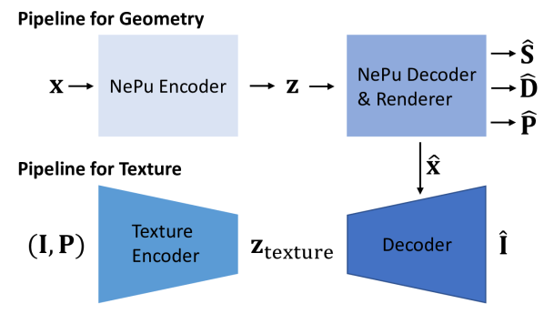
The heart of our framework is an encoder-decoder network that reconstructs the texture of an articulated shape, cf. Fig. 1. As a basis, we make use of Neural Puppeteer (NePu) [8] for neural rendering.
NePu is a neural rendering pipeline designed specifically for articulated shapes, which takes as input a set of 3D keypoints and a camera position, and maps them to a RGB image of the shape (similar to Fig. 1, top: Pipeline for Geometry). Notably, NePu renders in the 2D domain, which makes it much faster than volumetric rendering: via a transformer network, local features are computed for each keypoint (NePu Decoder in Fig. 1, top), which are then projected onto the image plane by the camera. Another attention-based network, the actual renderer, then generates a complete 2D image from the projected features at the keypoint locations (NePu Renderer in Fig. 1, top).
Our key idea in this work is to disentangle the pipelines for geometry and texture information of the shape that we call Neural Texture Puppeteer (NeTePu). Thus NeTePu, unlike NePu and [38, 30], can handle more than one texture in a single model. The original NePu pipeline is therefore modified to produce what we call a NNOPCS map (cf. Sec. 3.1) instead of a final image, cf. Fig. 1 (top). This NNOPCS map essentially encodes within the image plane the complete geometric information about the shape relevant for rendering this particular view. Local features (we refer to [8] and Sec. 3.1 for details) and global latent code (cf. Fig. 1, top) for the geometry are augmented with separate local features and a latent code for the texture map. An encoder network generates for a texture from a view of the shape, while the decoder is a second NePu-based renderer to generate the final image (cf. Fig. 1, bottom). Putting together the encoder and decoder for , we essentially obtain a texture auto-encoder which, given a fixed geometry, can be efficiently trained separately from the geometry network.
In the following subsections, we will give the details for these different modules.
3.1 Pipeline for Geometry
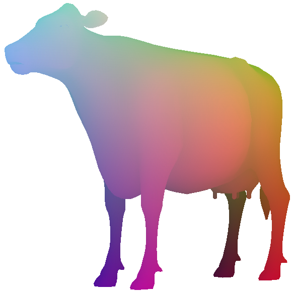
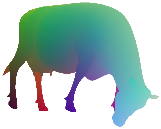
In our framework, the geometry and pose of an articulated shape is defined by the different keypoint locations and a single global latent code for the shape, which is decoded into a -dimensional local feature vector for each keypoint as input to the renderer. By varying the keypoint locations and keeping the features fixed, one can generate renderings of arbitrary poses of the same geometry [8]. We now use the rendering pipeline in [8], but do not interpret the output as a rendered color image. Instead, at each point in the image plane, the 3D output defines a 3D coordinate of a point on the shape in a normalized coordinate space (NOCS [46]), and additionally in a normalized neutral pose, cf. Fig. 2(a), which is why we denote it Normalized Neutral Object Pose and Coordinate Space (NNOPCS). Thus, the same point on the shape always has the same encoding, no matter the pose of the object and the camera view. The NNOPCS map can thus be viewed as a generalization of a NOCS map [46].
NNOPCS Maps for Articulated Shapes. Similar to [8], a coordinate on the object is defined via a 3D vector for each pixel of the target view with width and height , thus the NNOPCS map is a function of the form
| (1) |
Here, are the given camera extrinsics and intrinsics, respectively. The architecture remains the same, so we refer to [8] for details on how the function is implemented as an attention-based neural network. Similar to [46], the interpretation of the 3D output of the function in Eq. 1 is a dense pixel-NNOPCS correspondence. Ground truth data to learn the NNOPCS maps for articulated shapes end-to-end is rendered via Blender (www.blender.org), see section 4.
3.2 Pipeline for Texture
Texture Encoder. The texture of a shape is described by a -dimensional global texture latent code (same dimension as ), which augments the global geometry latent code , cf. Fig. 1. An encoder network computes from a masked input image together with the NNOPCS map (cf. Sec. 3.1) for a certain camera position,
| (2) |
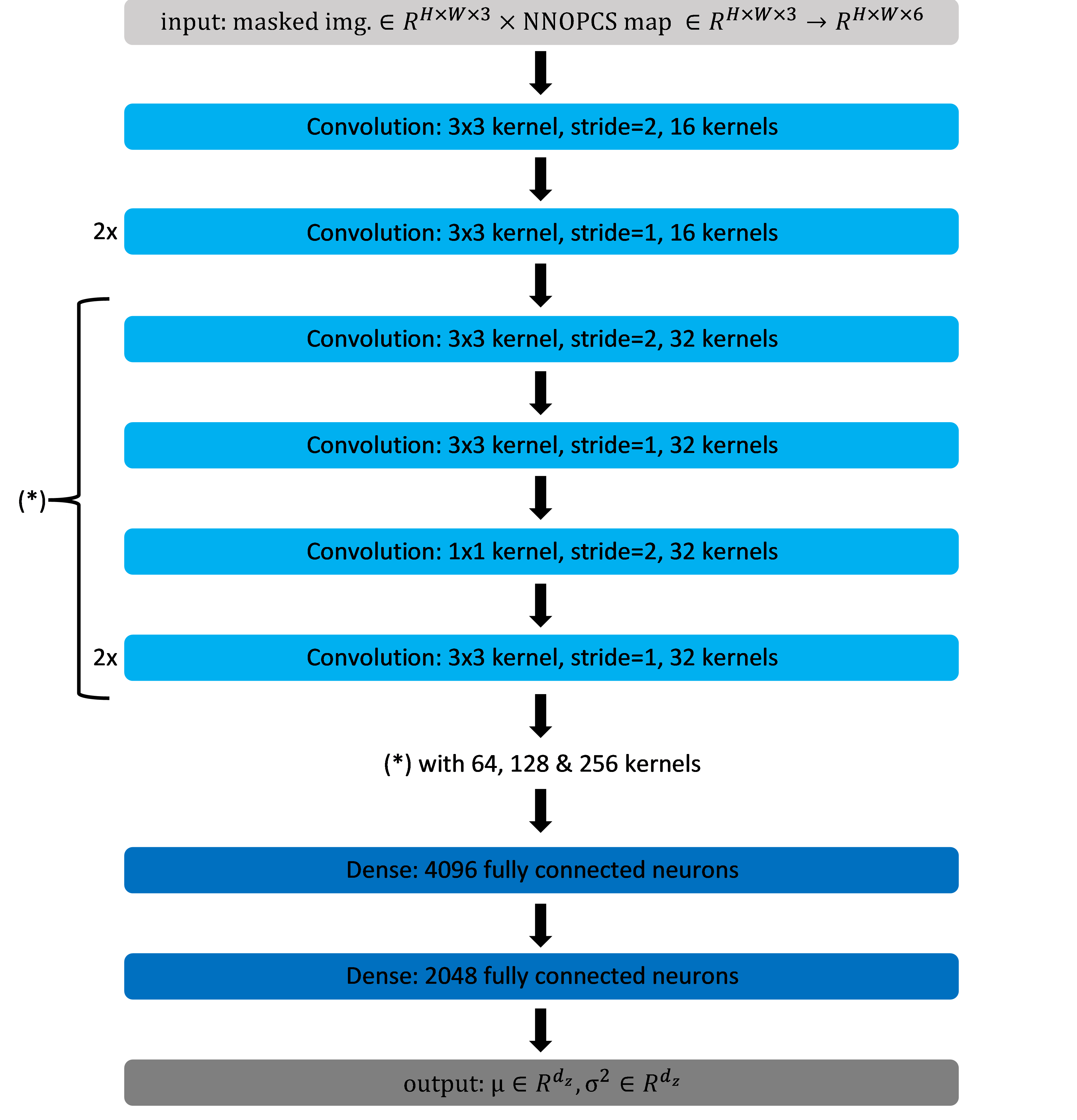
The texture encoder is implemented as a convolutional neural network with convolution and two dense layers. Between the layers we use batch normalization [12] and ReLu activations. Similar to a variational autoencoder [16], the texture encoder outputs a mean and standard deviation from which we sample the global texture latent code .
During training, we use the available ground truth NNOPCS maps (cf. Sec. 3.1) and silhouette masks. During inference, the silhouette mask and the NNOPCS map is estimated with the network trained above, cf. Fig. 1. Both the images as well as the NNOPCS maps are set to zero outside the shape’s silhouette.
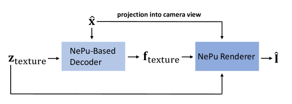
Neural Texture Rendering. Similar to how we render the NNOPCS maps (cf. Sec. 3.1), we first decode the global texture embedding from Eq. (2) into local texture features with a decoder network
| (3) |
where gives the -dimensional local texture features for each keypoint. Note that the dimension of is the same as the local geometry features , so the final renderer for a 2D image seen from camera view conditioned on and keypoints is again (compare with Eq. 1) a function of the form
| (4) |
4 Datasets and Training
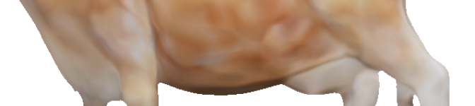
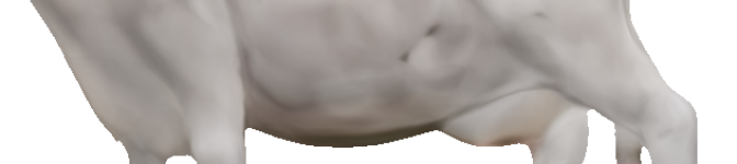
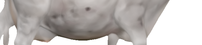
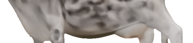
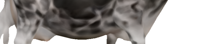
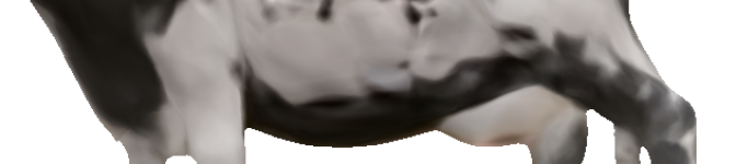
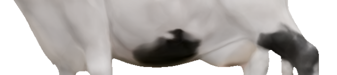
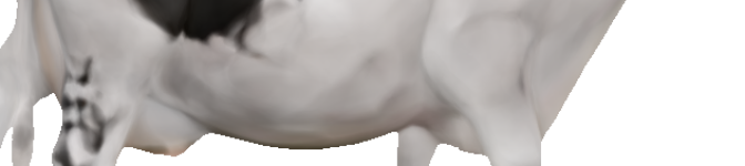
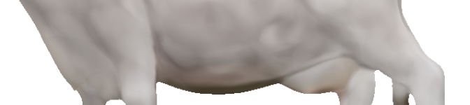
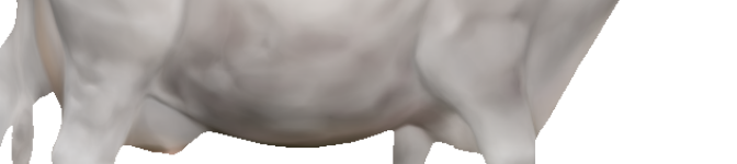
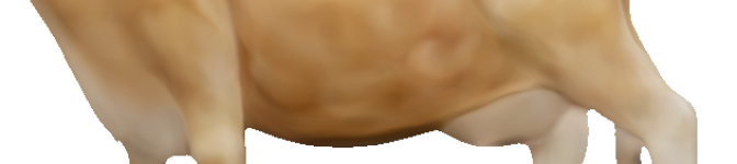
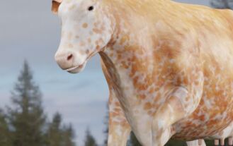
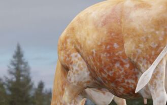
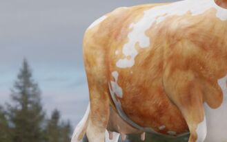
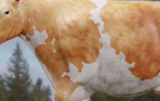
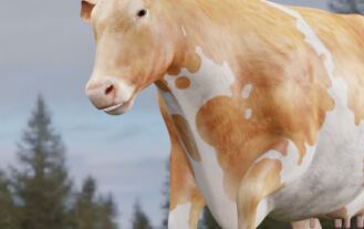
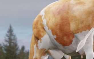
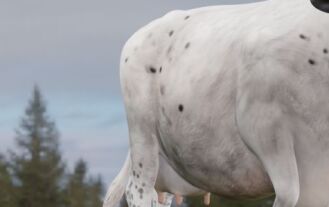
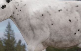
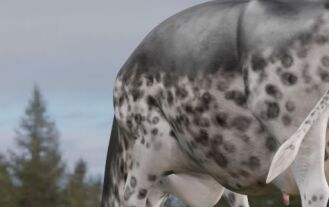
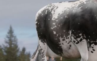
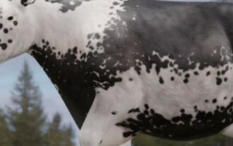
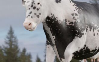
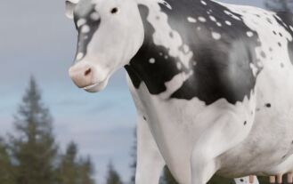
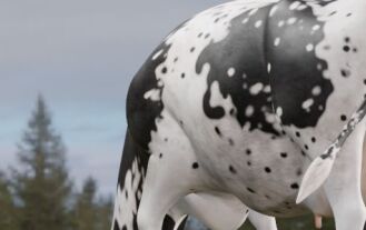
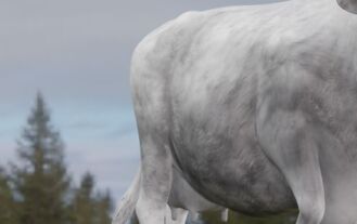
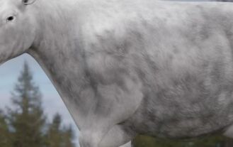
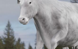
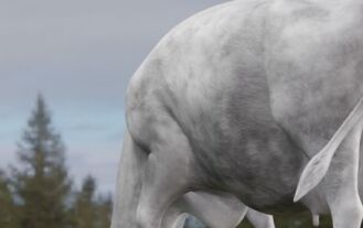
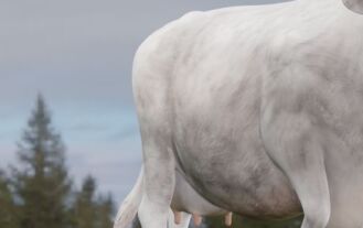
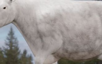
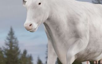
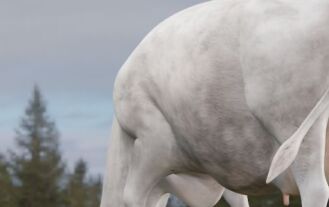
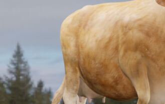
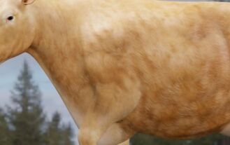
NePuMoo Dataset. For this proof of concept, we choose cows as an example shape because their textures can be clearly distinguished. We extend [9] with its Holstein cow texture by adding eleven additional cow textures. For each texture we provide the same poses, each captured from the same perspectives, placed in three evenly sampled rings at different heights around the model. This results in views per texture and a total of views. Each view consists of the ground truth 3D and 2D keypoints, the rendered RGB image, a silhouette of the cow, a depth map and a NNOPCS map, cf. Sec. 3.1. Each view has a resolution of px. All images were rendered using Blender (www.blender.org) and the Cycles rendering engine. We provide the same keypoints distributed among the joints of the cow as [9].
Our synthetic texture dataset also contains instances of occlusions. We generated instances captured from two of the camera views. In these samples the Holstein (texture ) partially occludes the Limousine (texture ) cow. For these cases we provide the occluded and complete silhouettes.
H36M Dataset. This human real-world dataset contains keypoint annotations, segmentations masks and RGB images of eleven actors in 17 scenarios, cf. [13]. We use the first frames of the “Posing” scenario from subjects (S1, S5, S6, S7, S8, S9, S11) for this study, similar to [30], and all four camera views for training.
Training the Pipeline for Geometry. To train the NNOPCS maps of articulated shapes, cf. Sec. 3.1, we use the same regimen as in [8]. However, instead of color images we train end-to-end with the ground truth NNOPCS map observations
| (5) |
over distinct poses captured by different cameras. All model parameters are trained jointly. In the composite loss from [8], instead of the color loss we define
| (6) |
which is the squared pixel-wise difference over all three channels. For the details of this equation and the composite loss, we refer to [8].
Training the Pipeline for Texture. While training our neural texture encoder, decoder and renderer (cf. Fig. 1, bottom), we keep the weights of the pipeline for geometry (cf. Fig. 1, top) fixed and use the ground truth NNOPCS as the fixed geometry. We thus learn only the texture relevant weights of the pipeline in this step.
Assuming the dataset has textures with images provided for each texture and the same poses and cameras as the NNOPCS maps, we define the color rendering loss
| (7) |
as the squared pixel-wise difference over all color channels, where is the color rendering function from [8] defined in Eq. (4). To regularize the texture latent space, we employ the Kullback–Leibler divergence [17] between the predicted multi-dimensional normal distribution and the standard normal distribution. We enforce this loss with the same sampling scheme and reparametrization trick as in the training of a variational autoencoder [16]. The total loss is thus
| (8) |
where the different positive numbers are hyperparameters to balance the influence of the two losses.
5 Experiments
In Sec. 5.1 we provide implementation details of our architecture from Sec. 3. We then evaluate the learned NNOPCS maps (cf. Sec. 3.1) in Sec. 5.2. In Sec. 5.3 we show novel pose synthesis on our novel NePuMoo and the H36M [13] dataset and provide texture reconstructions of a real-world example with a model trained on synthetic data only. In Sec. 5.4 you find our kernel density estimation (KDE) [35, 29] of the t-SNE [41] of the global texture embedding that we compare to the embedding of [11].
5.1 Implementation Details
To train NeTePu, we extend the training procedure and parameters from [8]. We do not render complete NNOPCS (cf. Sec. 3.1) and texture maps to compute and during training, as this would be too costly. Instead, we choose points in each iteration that we sample uniformly within the ground truth mask. For the cow shape we increase the number of nearest neighbours in the vector cross-attention (VCA) module from to as we observe better performance (cf. Tab. 1).
Pipeline for Geometry. While training the NNOPCS maps, we also learn to reconstruct masks and depth, just as in [8]. However, in contrast to [8], we choose to use the 2-norm (vs. MSE in [8]) as depth loss during training which leads to better results in terms of MAE, cf. Tab. 1.
| NNOPCS Maps MSE | Depth MAE [mm] | ||||||||
|---|---|---|---|---|---|---|---|---|---|
|
|
Pipeline for Texture. We train the neural texture rendering pipeline using an initial learning rate of , which is decayed with a factor of on our novel NePuMoo dataset and on the H36M dataset [13] every epochs. We choose final weights based on the minimum validation loss, i.e. epoch for our NePuMoo and for the H36M dataset. We weight the training loss in Eq. (8) with and .
5.2 NNOPCS Maps


Quantitative results for the NNOPCS map (cf. Sec. 3.1) estimation are shown in Tab. 1. Over all cow test samples, we achieve a mean squared error (MSE) of . Since the coordinates of the NNOPCS are normalized to this means that our learned NNOPCS maps have an error of on average. This overall high quality is also reflected in our qualitative example in Fig. 2(b), and is a necessary step in order to achieve accurate texture renderings.
5.3 Neural Texture Rendering
| Dataset / Metric | Color PSNR [dB] |
|---|---|
| H36M [13] | |
| NePuMoo |
Quantitative results for novel pose synthesis are shown in Tab. 2. We report the PSNR [dB] over all test samples for our reconstructed RGB images on the real-world H36M [13] and our NePuMoo test set.
We achieve an overall PSNR of on our novel NePuMoo data. This is slightly better than the PSNR of reported in [8] although in contrast to [8], we render twelve textures instead of one with a single model.
On the H36M data [13] we achieve an overall PSNR of . See Fig. 6 (right pair) for a qualitative example. Please note that the H36M data does not provide NNOPCS maps (cf. Sec. 3.1) and we thus train NeTePu without them. In this case NeTePu can not leverage the geometric shape information provided by the NNOPCS maps. This holds for any data that does not provide NNOPCS maps. For a deeper insight on the influence and the importance of the NNOPCS maps, we refer to our ablation studies.
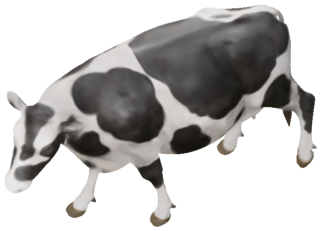
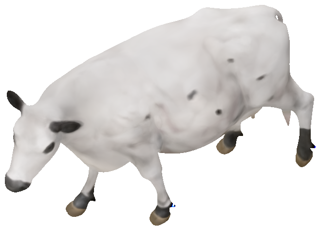
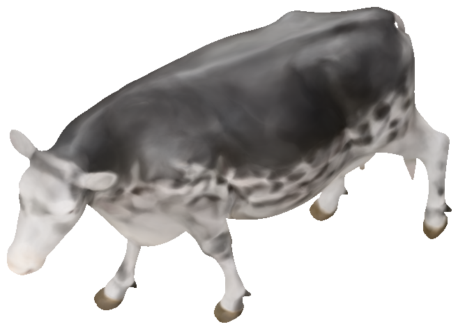
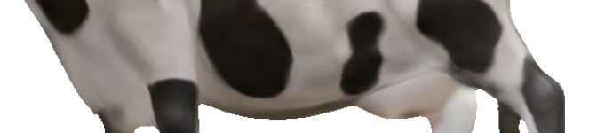
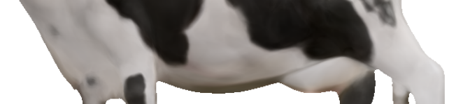
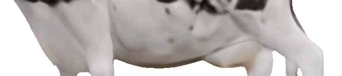
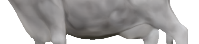
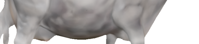
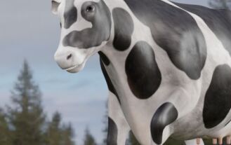
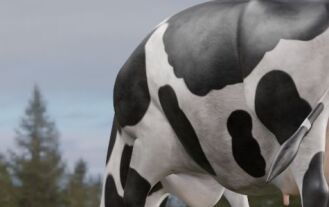
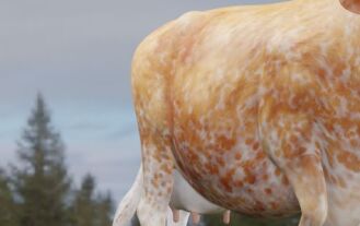
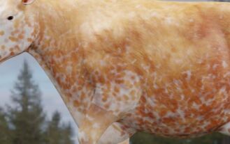
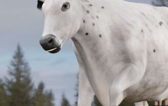
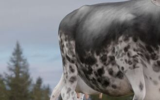
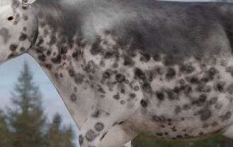
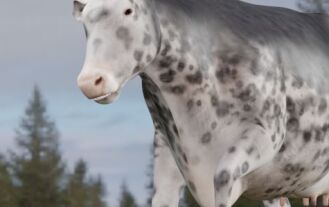
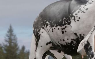
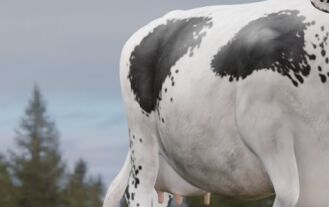
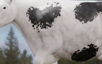
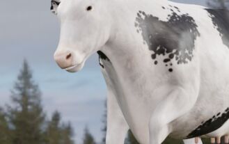
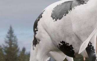
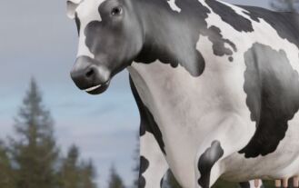
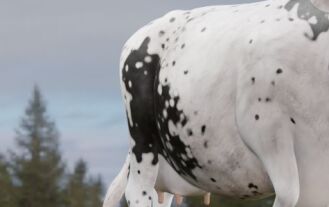
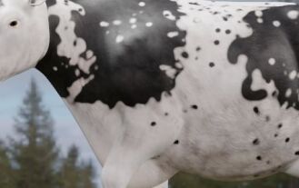
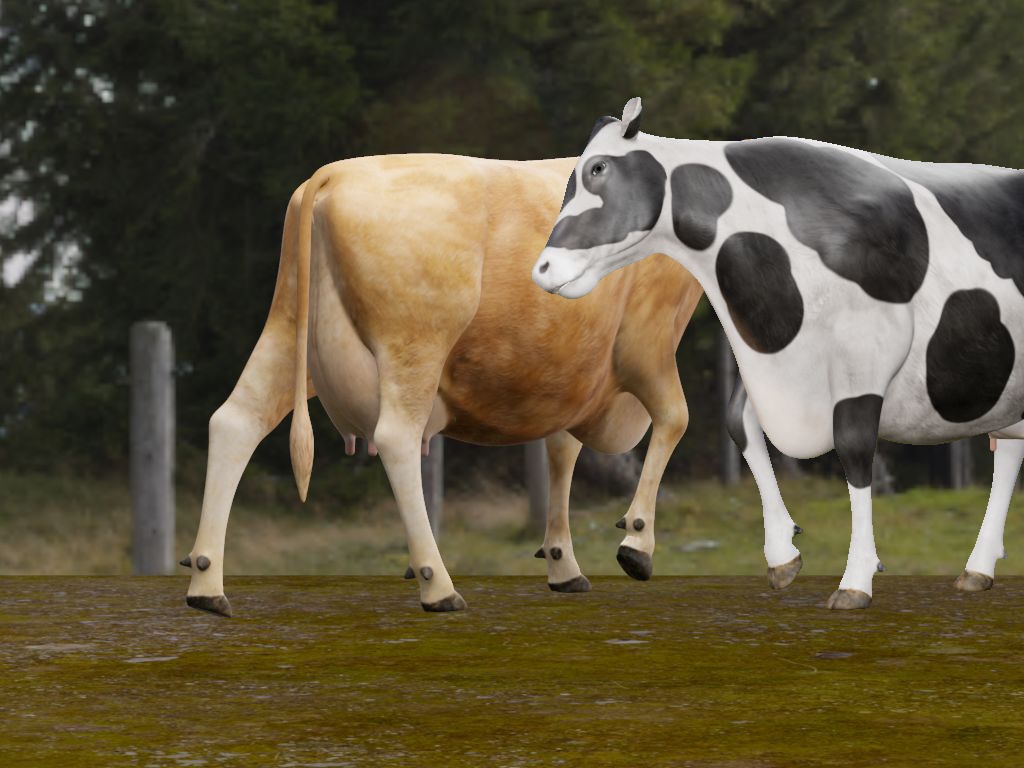
We reconstruct images for novel views and novel poses from our NePuMoo test set, which have not been seen during training. In Fig. 3 we show two examples for each distinct texture in our dataset. The reconstructions look realistic and contain details like the black freckles of texture and (cf. eg. Fig. 3(f)) or the black legs, ears and nose tip of texture (cf. Fig. 3(d)). The dataset contains two challenging texture pairs, which are difficult to distinguish by eye. We note that even these challenging texture pairs , and , are reconstructed correctly (cf. Figs. 3(j) and 3(k) and Figs. 3(b) and 3(l) respectively).
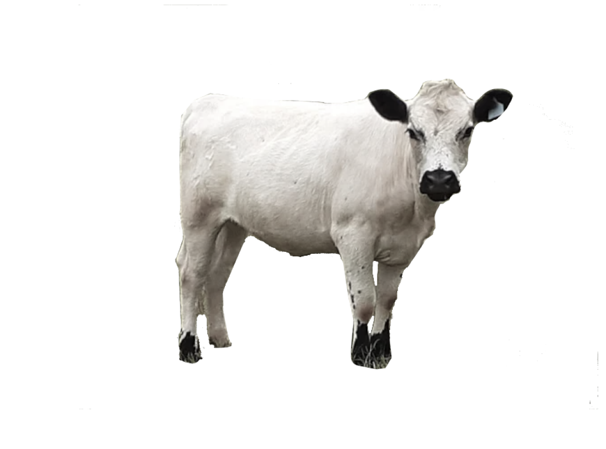
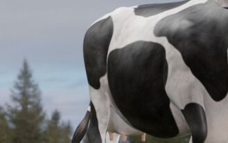
We also perform a texture domain shift from synthetic to real. For this, we use the model that we train on our novel NePuMoo texture dataset and infer a zero-shot synthetic to real-world example. Our reconstructions are shown in Fig. 4. We reconstruct the texture of the real-world image for three different poses (cf. Fig. 4(b)). Even though only trained with synthetic data, this shows that NeTePu can be used for real-world applications that do not provide NNOPCS maps, cf. Sec. 3.1. This makes our model useful for real-world applications with endangered animal species where available real-world data is limited.
Ablation Studies.
| Color PSNR [dB] | |
|---|---|
| w/o NNOPCS Maps | |
| w/ NNOPCS Maps |
To evaluate the influence of the NNOPCS maps (cf. Sec. 3.1) we run an experiment on our novel NePuMoo dataset with the same parameters as specified in Sec. 5.1. The only difference is that we do not use NNOPCS maps in our pipeline, cf. Fig. 1. We report the color PSNR over all test samples in Tab. 3. If our model can leverage geometric information of the shape that is provided by the NNOPCS maps, NeTePu achieves a better color PSNR on average by . This quantitative difference is visible in the qualitative results, cf. Fig. 6 (left pair). This also explains the quality of our results on the H36M dataset [13], cf. Tabs. 2 and 6 (right pair).
We perform another ablation study on the influence of the local texture features . We run an experiment on our novel NePuMoo data where we do not augment the local features for geometry with local features for texture . We see that augmenting the local features for geometry with achieves a better color PSNR on average by dB ( dB in Tab. 2 vs. dB).
5.4 Re-identification
Our proposed neural rendering pipeline learns a global texture embedding which can be used to identify individuals. This is a valuable task for applications that need re-identification of individuals like tracking scenarios where the tracked object leaves and re-enters the scene. For this task, we use Eq. (2) to encode a global latent vector that describes the texture of individual observed from camera view in pose . In this way, we can generate a global texture embedding (capital Z) for all individuals under consideration from our learned NNOPCS maps (cf. Sec. 3.1) and masked 2D color observations ,
| (9) |
Baseline. For a comparison, we train TransReID [11] on our novel NePuMoo data, cf. Sec. 4. [11] is a transformer-based framework for object re-identification that is optimized with ID [52] and triplet loss [21]. During training [11] needs positive and negative pairs of the object. We resize the input to px and use a batch size of . For the other parameters we use their standard. After training, we generate a global feature embedding with their global features for a comparison.
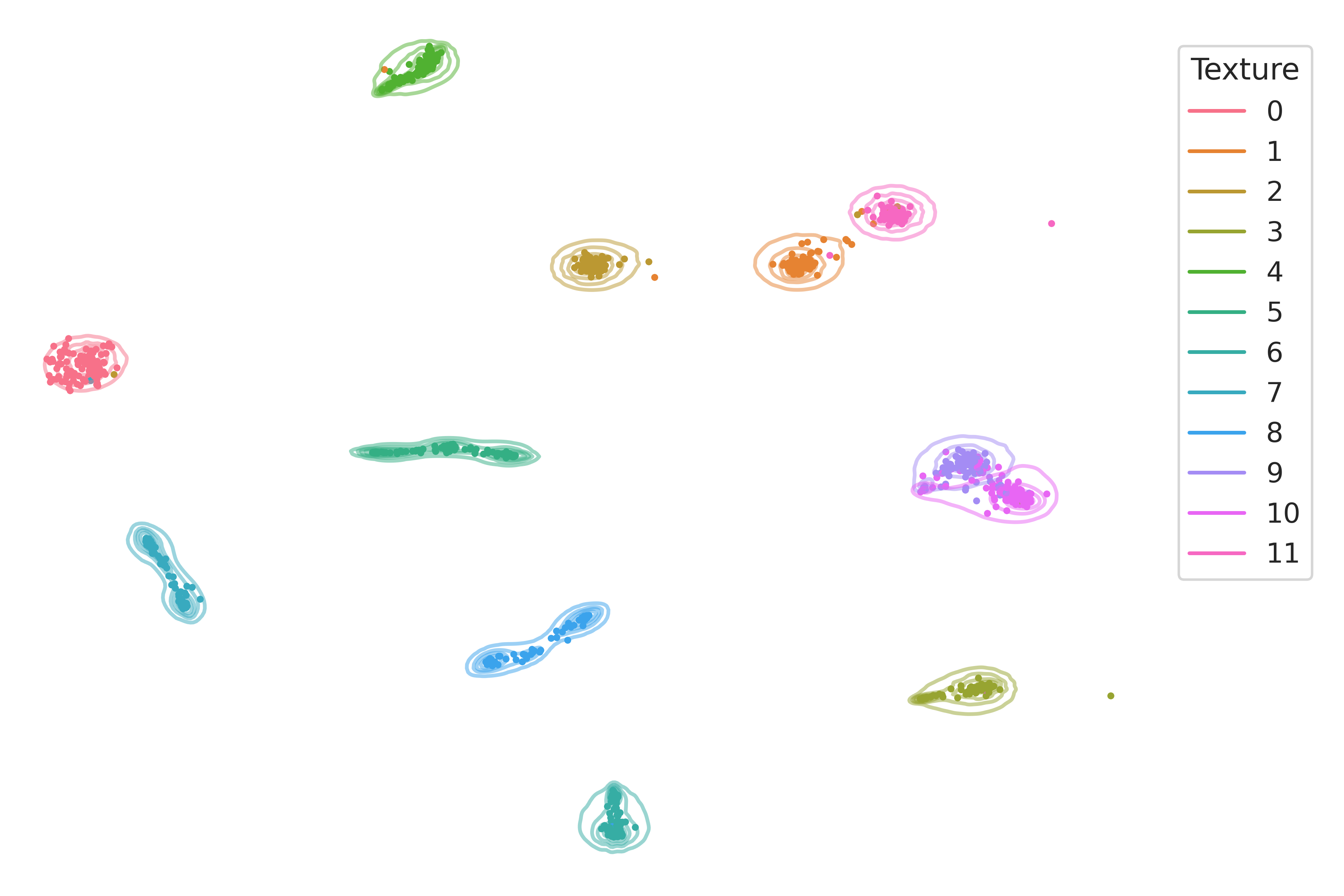
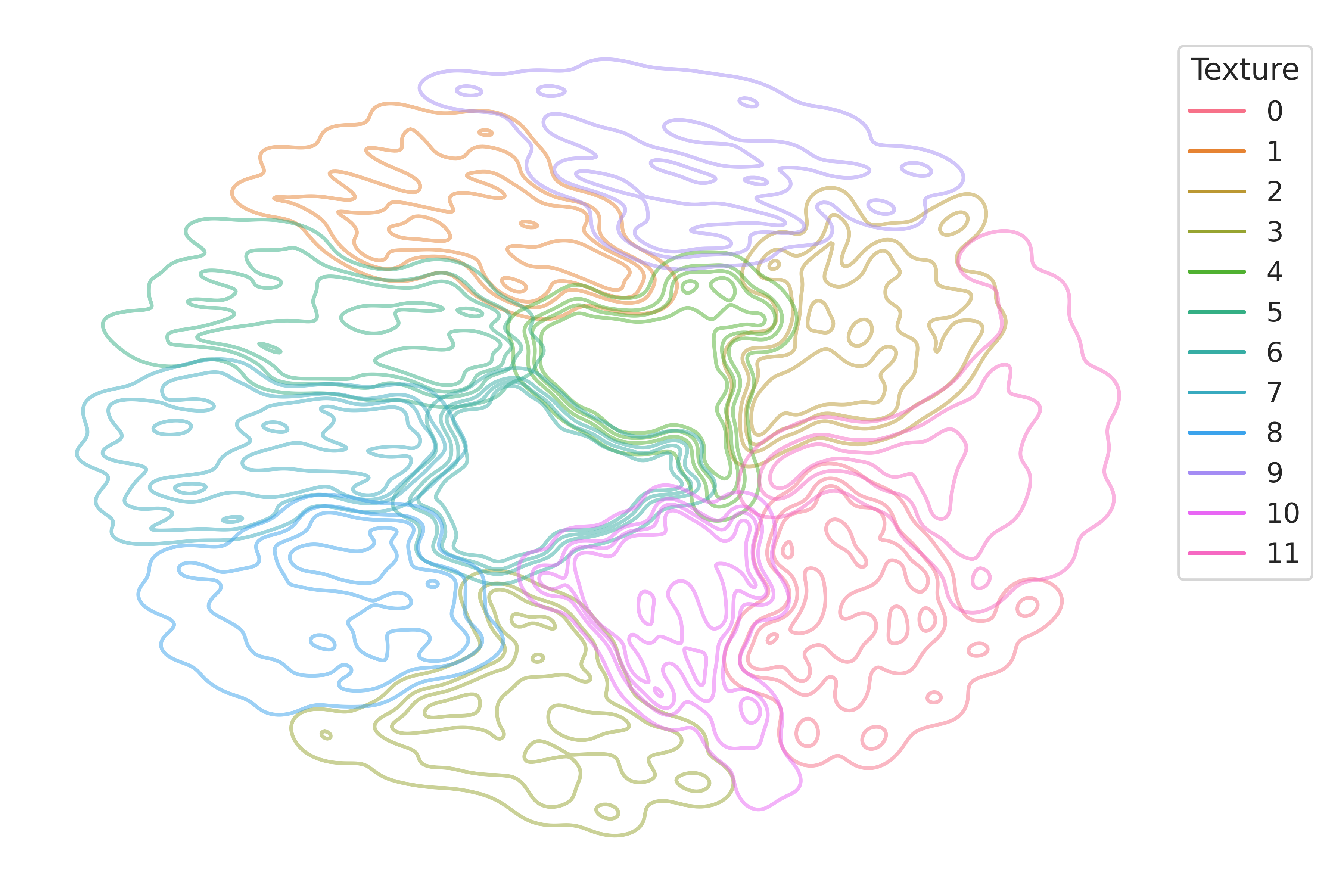


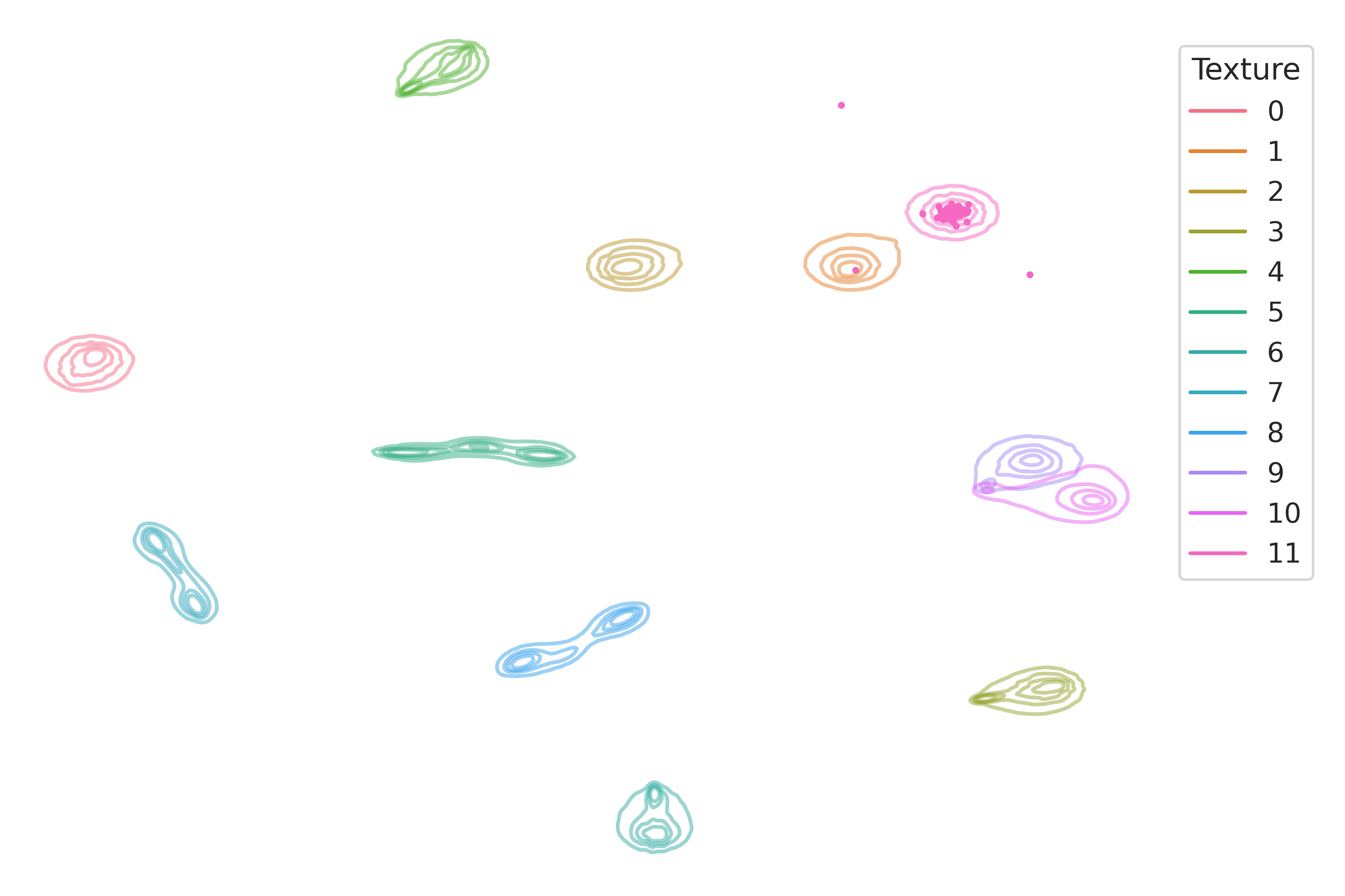
Results. In Fig. 5(a) we show NeTePu’s kernel density estimation (KDE) [35, 29] of the t-SNE [41] of the global texture embedding from Eq. (9) of twelve cows from our novel synthetic NePuMoo dataset (cf. Sec. 4). We encode the global texture codes of all poses, twelve textures and cameras. While the contour lines show the distribution of global texture codes for the camera views from our dataset, the dots show the global codes for novel camera views. In Fig. 5(b) we show the KDE of the global feature embedding generated with [11] for a comparison.
We see that the textures cluster in such a way that they can be distinguished by both frameworks. Both frameworks can distinguish the challenging textures and (cf. Figs. 3(b) and 3(l)) and and (cf. Figs. 3(j) and 3(k)). While the embedding of [11] is more compact, we observe only one slight overlap of texture clusters for NeTePu. No cluster overlap in the embedding helps in readily distinguishing all textures in all poses from all camera views. Furthermore, note that NeTePu’s global texture latent codes of novel camera views (dots in Fig. 5(a)) fall into the corresponding clusters of the known camera views (contour lines in Fig. 5(a)).
Runtime. We evaluate the runtime on our novel NePuMoo dataset with a workstation that has a nVidia Titan RTX, 64 GB DDR4 RAM, an Intel Xeon E5-2620 at 2.10GHz and a 2TB Samsung SSD 850. We encode the global texture code from an input of size (masked 2D color observation and learned NNOPCS map, cf. Sec. 3.1). This calculation includes to render our learned NNOPCS maps with a resolution of . Since our NNOPCS maps are only defined within the object, the calculation also includes to render the learned mask with a resolution of . We use a batch size of for all twelve textures of samples from our dataset seen from camera views. In total, we thus encode the global texture code for frames. To calculate the runtime, we take the average over these frames. We achieve a runtime of fps.
All together, this is why our proposed neural rendering pipeline offers an alternative approach to CNN- or transformer-based frameworks like [11] for the task of re-identification in interactive tracking applications.
6 Limitations and Future Work
At the moment, we learn the NNOPCS maps in a supervised manner, cf. Sec. 3.1. This limits our method to data that provide NNOPCS maps. If we train on data that does not provide these NNOCPS maps, the quality of the outcome diminishs because the model lacks information on the geometry’s shape, cf. Fig. 6. In order to make our method more applicable, especially to real-world applications, we aim to learn the NNOPCS maps in the future in an unsupervised manner. Also, at this point our dataset contains a limited variety of textures. In the future we aim at extending our dataset to allow for better generalizability when it comes to new - unseen - textures.
7 Conclusions
In this paper, we present a neural rendering pipeline for textured articulated shapes. We show that NeTePu encodes a distinct global texture embedding (cf. Fig. 5(a)), which is computed from a learned NNOPCS map (cf. Sec. 3.1) and 2D color information. This global texture embedding can be used in a downstream task to identify individuals. Our neural rendering-based re-identification process runs at interactive speed (cf. Sec. 5.4), and thus offers an alternative to CNN- or transformer-based approaches like [11] in tracking applications. To the best of our knowledge, we are the first to provide a framework for re-identification of articulated individuals based on neural rendering. We also demonstrate NeTePu’s quality with realistic looking novel view and pose synthesis for different synthetic cow textures, cf. Fig. 3. Restricted by the availability of ground truth NNOPCS maps, the quality for real-world data synthesis is reduced, cf. Fig. 6 (right pair). We further demonstrate the flexibility of our model by applying a synthetic to real-world texture domain shift where we reconstruct the texture from a real-world 2D RGB image with a model trained on synthetic data only. This makes our model useful for real-world applications with endangered animal species where available real-world data is limited and synthetic data can be generated using Blender (www.blender.org).
We hope that this work inspires other researchers to develop methods for neural rendering-based re-identification which work for humans and animals.
Acknowledgements. We acknowledge funding by the Deutsche Forschungsgemeinschaft (DFG, German Research Foundation) under Germany’s Excellence Strategy – EXC 2117 – 422037984, and the Federal Ministry of Education and Research (BMBF) within the research program – KI4KMU – 01IS23046B.
References
- [1] Praneet C. Bala, Benjamin R. Eisenreich, Seng Bum Michael Yoo, Benjamin Y. Hayden, Hyun Soo Park, and Jan Zimmermann. Automated markerless pose estimation in freely moving macaques with openmonkeystudio. Nat. Commun., 11:4560, 2020.
- [2] Alex Bewley, Zongyuan Ge, Lionel Ott, Fabio Ramos, and Ben Upcroft. Simple online and realtime tracking. In ICIP, pages 3464–3468, 2016.
- [3] Long Chen, Haizhou Ai, Rui Chen, Zijie Zhuang, and Shuang Liu. Cross-view tracking for multi-human 3d pose estimation at over 100 fps. In CVPR, pages 3279–3288, 2020.
- [4] Gioele Ciaparrone, Francisco Luque Sánchez, Siham Tabik, Luigi Troiano, Roberto Tagliaferri, and Francisco Herrera. Deep learning in video multi-object tracking: A survey. Neurocomputing, 381:61–88, 2020.
- [5] Ying Cui, Dongyan Guo, Yanyan Shao, Zhenhua Wang, Chunhua Shen, Liyan Zhang, and Shengyong Chen. Joint classification and regression for visual tracking with fully convolutional siamese networks. IJCV, pages 1–17, 2022.
- [6] Patrick Dendorfer, Aljosa Osep, Anton Milan, Konrad Schindler, Daniel Cremers, Ian Reid, Stefan Roth, and Laura Leal-Taixé. Motchallenge: A benchmark for single-camera multiple target tracking. IJCV, 129(4):845–881, 2021.
- [7] André C Ferreira, Liliana R Silva, Francesco Renna, Hanja B Brandl, Julien P Renoult, Damien R Farine, Rita Covas, and Claire Doutrelant. Deep learning-based methods for individual recognition in small birds. Methods in Ecology and Evolution, 11(9):1072–1085, 2020.
- [8] Simon Giebenhain, Urs Waldmann, Ole Johannsen, and Bastian Goldluecke. Neural puppeteer: Keypoint-based neural rendering of dynamic shapes. In Proceedings of the Asian Conference on Computer Vision (ACCV), pages 2830–2847, December 2022.
- [9] Simon Giebenhain, Urs Waldmann, Ole Johannsen, and Bastian Goldlücke. Neural puppeteer: Keypoint-based neural rendering of dynamic shapes (datset), October 2022.
- [10] Yaning Han, Ke Chen, Yunke Wang, Wenhao Liu, Xiaojing Wang, Jiahui Liao, Yiting Huang, Chuanliang Han, Kang Huang, Jiajia Zhang, et al. Social behavior atlas: A computational framework for tracking and mapping 3d close interactions of free-moving animals. bioRxiv, pages 2023–03, 2023.
- [11] Shuting He, Hao Luo, Pichao Wang, Fan Wang, Hao Li, and Wei Jiang. Transreid: Transformer-based object re-identification. In ICCV, pages 15013–15022, 2021.
- [12] Sergey Ioffe and Christian Szegedy. Batch normalization: Accelerating deep network training by reducing internal covariate shift. In Francis Bach and David Blei, editors, Proceedings of the 32nd International Conference on Machine Learning, volume 37 of Proceedings of Machine Learning Research, pages 448–456, Lille, France, 07–09 Jul 2015. PMLR.
- [13] Catalin Ionescu, Dragos Papava, Vlad Olaru, and Cristian Sminchisescu. Human3.6m: Large scale datasets and predictive methods for 3d human sensing in natural environments. IEEE TPAMI, 36(7):1325–1339, 2014.
- [14] Angjoo Kanazawa, Shubham Tulsiani, Alexei A. Efros, and Jitendra Malik. Learning category-specific mesh reconstruction from image collections. In ECCV, September 2018.
- [15] Roland Kays, Margaret C. Crofoot, Walter Jetz, and Martin Wikelski. Terrestrial animal tracking as an eye on life and planet. Science, 348(6240):aaa2478, 2015.
- [16] Diederik P. Kingma and Max Welling. Auto-Encoding Variational Bayes. In 2nd International Conference on Learning Representations, ICLR 2014, Banff, AB, Canada, April 14-16, 2014, Conference Track Proceedings, 2014.
- [17] Solomon Kullback and Richard A Leibler. On information and sufficiency. The annals of mathematical statistics, 22(1):79–86, 1951.
- [18] Jessy Lauer, Mu Zhou, Shaokai Ye, William Menegas, Steffen Schneider, Tanmay Nath, Mohammed Mostafizur Rahman, Valentina Di Santo, Daniel Soberanes, Guoping Feng, Venkatesh N. Murthy, George Lauder, Catherine Dulac, Mackenzie W. Mathis, and Alexander Mathis. Multi-animal pose estimation, identification and tracking with deeplabcut. Nat. Methods, 19:496–504, 2022.
- [19] Xueting Li, Sifei Liu, Kihwan Kim, Shalini De Mello, Varun Jampani, Ming-Hsuan Yang, and Jan Kautz. Self-supervised single-view 3d reconstruction via semantic consistency. In Andrea Vedaldi, Horst Bischof, Thomas Brox, and Jan-Michael Frahm, editors, ECCV, pages 677–693, Cham, 2020. Springer International Publishing.
- [20] Chen-Hsuan Lin, Chaoyang Wang, and Simon Lucey. Sdf-srn: Learning signed distance 3d object reconstruction from static images. NeurIPS, 33:11453–11464, 2020.
- [21] Hao Liu, Jiashi Feng, Meibin Qi, Jianguo Jiang, and Shuicheng Yan. End-to-end comparative attention networks for person re-identification. IEEE Transactions on Image Processing, 26(7):3492–3506, 2017.
- [22] Ze Liu, Yingfeng Cai, Hai Wang, Long Chen, Hongbo Gao, Yunyi Jia, and Yicheng Li. Robust target recognition and tracking of self-driving cars with radar and camera information fusion under severe weather conditions. IEEE Transactions on Intelligent Transportation Systems, 23(7):6640–6653, 2021.
- [23] Matthew Loper, Naureen Mahmood, Javier Romero, Gerard Pons-Moll, and Michael J. Black. Smpl: A skinned multi-person linear model. ACM Trans. Graph., 34(6), oct 2015.
- [24] Matthew M Loper and Michael J Black. Opendr: An approximate differentiable renderer. In ECCV, pages 154–169. Springer, 2014.
- [25] Jesse D Marshall, Ugne Klibaite, Amanda Gellis, Diego E Aldarondo, Bence P Ölveczky, and Timothy W Dunn. The pair-r24m dataset for multi-animal 3d pose estimation. bioRxiv, pages 2021–11, 2021.
- [26] Ben Mildenhall, Pratul P. Srinivasan, Matthew Tancik, Jonathan T. Barron, Ravi Ramamoorthi, and Ren Ng. Nerf: Representing scenes as neural radiance fields for view synthesis. In ECCV, 2020.
- [27] Hemal Naik, Alex Hoi Hang Chan, Junran Yang, Mathilde Delacoux, Iain D. Couzin, Fumihiro Kano, and Máté Nagy. 3d-pop - an automated annotation approach to facilitate markerless 2d-3d tracking of freely moving birds with marker-based motion capture. In CVPR, pages 21274–21284, June 2023.
- [28] Michael Niemeyer, Lars Mescheder, Michael Oechsle, and Andreas Geiger. Differentiable volumetric rendering: Learning implicit 3d representations without 3d supervision. In CVPR, pages 3504–3515, 2020.
- [29] Emanuel Parzen. On Estimation of a Probability Density Function and Mode. The Annals of Mathematical Statistics, 33(3):1065 – 1076, 1962.
- [30] Sida Peng, Junting Dong, Qianqian Wang, Shangzhan Zhang, Qing Shuai, Xiaowei Zhou, and Hujun Bao. Animatable neural radiance fields for modeling dynamic human bodies. In ICCV, pages 14314–14323, October 2021.
- [31] Sida Peng, Yuanqing Zhang, Yinghao Xu, Qianqian Wang, Qing Shuai, Hujun Bao, and Xiaowei Zhou. Neural body: Implicit neural representations with structured latent codes for novel view synthesis of dynamic humans. In CVPR, 2021.
- [32] Talmo D. Pereira, Nathaniel Tabris, Arie Matsliah, David M. Turner, Junyu Li, Shruthi Ravindranath, Eleni S. Papadoyannis, Edna Normand, David S. Deutsch, Z. Yan Wang, Grace C. McKenzie-Smith, Catalin C. Mitelut, Marielisa Diez Castro, John D’Uva, Mikhail Kislin, Dan H. Sanes, Sarah D. Kocher, Samuel S.-H. Wang, Annegret L. Falkner, Joshua W. Shaevitz, and Mala Murthy. Sleap: A deep learning system for multi-animal pose tracking. Nat. Methods, 19:486–495, 2022.
- [33] Umer Rafi, Andreas Doering, Bastian Leibe, and Juergen Gall. Self-supervised keypoint correspondences for multi-person pose estimation and tracking in videos. In ECCV, pages 36–52. Springer International Publishing, 2020.
- [34] Jathushan Rajasegaran, Georgios Pavlakos, Angjoo Kanazawa, and Jitendra Malik. Tracking people by predicting 3d appearance, location and pose. In CVPR, pages 2740–2749, 2022.
- [35] Murray Rosenblatt. Remarks on Some Nonparametric Estimates of a Density Function. The Annals of Mathematical Statistics, 27(3):832 – 837, 1956.
- [36] Shunsuke Saito, Zeng Huang, Ryota Natsume, Shigeo Morishima, Angjoo Kanazawa, and Hao Li. Pifu: Pixel-aligned implicit function for high-resolution clothed human digitization. In ICCV, pages 2304–2314, 2019.
- [37] Vincent Sitzmann, Semon Rezchikov, William T. Freeman, Joshua B. Tenenbaum, and Fredo Durand. Light field networks: Neural scene representations with single-evaluation rendering. In Advances in Neural Information Processing Systems, 2021.
- [38] Shih-Yang Su, Frank Yu, Michael Zollhöfer, and Helge Rhodin. A-nerf: Articulated neural radiance fields for learning human shape, appearance, and pose. In NeurIPS, 2021.
- [39] Ayush Tewari, Ohad Fried, Justus Thies, Vincent Sitzmann, Stephen Lombardi, Kalyan Sunkavalli, Ricardo Martin-Brualla, Tomas Simon, Jason Saragih, Matthias Nießner, et al. State of the art on neural rendering. In Computer Graphics Forum, volume 39, pages 701–727. Wiley Online Library, 2020.
- [40] Ayush Tewari, Justus Thies, Ben Mildenhall, Pratul Srinivasan, Edgar Tretschk, Wang Yifan, Christoph Lassner, Vincent Sitzmann, Ricardo Martin-Brualla, Stephen Lombardi, et al. Advances in neural rendering. In Computer Graphics Forum, volume 41, pages 703–735. Wiley Online Library, 2022.
- [41] Laurens van der Maaten and Geoffrey Hinton. Visualizing data using t-sne. Journal of Machine Learning Research, 9(86):2579–2605, 2008.
- [42] Urs Waldmann, Jannik Bamberger, Ole Johannsen, Oliver Deussen, and Bastian Goldlücke. Improving unsupervised label propagation for pose tracking and video object segmentation. In DAGM German Conference on Pattern Recognition, pages 230–245. Springer, 2022.
- [43] Urs Waldmann, Alex Hoi Hang Chan, Hemal Naik, Máté Nagy, Iain D Couzin, Oliver Deussen, Bastian Goldluecke, and Fumihiro Kano. 3d-muppet: 3d multi-pigeon pose estimation and tracking. arXiv preprint arXiv:2308.15316, 2023.
- [44] Urs Waldmann, Hemal Naik, Nagy Máté, Fumihiro Kano, Iain D Couzin, Oliver Deussen, and Bastian Goldlücke. I-muppet: Interactive multi-pigeon pose estimation and tracking. In DAGM German Conference on Pattern Recognition, pages 513–528. Springer, 2022.
- [45] Tristan Walter and Iain D Couzin. Trex, a fast multi-animal tracking system with markerless identification, and 2d estimation of posture and visual fields. eLife, 10:e64000, 2021.
- [46] He Wang, Srinath Sridhar, Jingwei Huang, Julien Valentin, Shuran Song, and Leonidas J Guibas. Normalized object coordinate space for category-level 6d object pose and size estimation. In CVPR, pages 2642–2651, 2019.
- [47] Jian Wang, Yunshan Zhong, Yachun Li, Chi Zhang, and Yichen Wei. Re-identification supervised texture generation. In CVPR, pages 11846–11856, 2019.
- [48] Shangzhe Wu, Ruining Li, Tomas Jakab, Christian Rupprecht, and Andrea Vedaldi. Magicpony: Learning articulated 3d animals in the wild. In CVPR, pages 8792–8802, 2023.
- [49] Yiheng Xie, Towaki Takikawa, Shunsuke Saito, Or Litany, Shiqin Yan, Numair Khan, Federico Tombari, James Tompkin, Vincent Sitzmann, and Srinath Sridhar. Neural fields in visual computing and beyond. In Computer Graphics Forum, volume 41, pages 641–676. Wiley Online Library, 2022.
- [50] Alper Yilmaz, Omar Javed, and Mubarak Shah. Object tracking: A survey. Acm computing surveys (CSUR), 38(4):13–es, 2006.
- [51] Wentao Yuan, Zhaoyang Lv, Tanner Schmidt, and Steven Lovegrove. Star: Self-supervised tracking and reconstruction of rigid objects in motion with neural rendering. In CVPR, pages 13144–13152, 2021.
- [52] Zhedong Zheng, Liang Zheng, and Yi Yang. A discriminatively learned cnn embedding for person reidentification. ACM transactions on multimedia computing, communications, and applications (TOMM), 14(1):1–20, 2017.
- [53] Silvia Zuffi, Angjoo Kanazawa, Tanya Berger-Wolf, and Michael J. Black. Three-d safari: Learning to estimate zebra pose, shape, and texture from images ”in the wild”. In ICCV, October 2019.
- [54] Silvia Zuffi, Angjoo Kanazawa, and Michael J. Black. Lions and tigers and bears: Capturing non-rigid, 3d, articulated shape from images. In CVPR, 2018.
Appendix A Architecture
As mentioned in the main paper, our key idea in this work is to disentangle the pipelines for geometry and texture information of the shape.
The original NePu [8] pipeline is modified (cf. Fig. 7, top) to produce a NNOPCS map (cf. Sec. 3.1 in main paper, similar to [46]) instead of a final image, which essentially encodes within the image plane the complete geometric information about the shape relevant for rendering this particular view. In addition, we also predict the silhouette and depth map like the original NePu pipeline.
The heart of our framework is an encoder-decoder network for the texture of an articulated shape (cf. Fig. 7, bottom). The detailed architecture of our texture encoder (cf. Fig. 7, bottom left) can be found in Fig. 8. Fig. 9 shows the decoder (cf. Fig. 7, bottom right) in more detail.
A.1 Additional Implementation Details
As mentioned in the main paper, in order to disentangle geometry and texture (cf. Fig. 7), we augment the local and global features for geometry and , respectively, with local and global features and , respectively, for the texture. In all experiments, we choose and . For the other implementation details, we refer to [8].
A.2 Additional Ablation Study
| Color PSNR [dB] | |
|---|---|
| w/o | |
| w/ |
We perform an ablation study on the influence of the local texture features . We run an experiment on our novel NePuMoo data where we do not augment the local features for geometry with local features for texture . In Tab. 4 we report the color PSNR [dB] over all NePuMoo test samples. We see that augmenting the local features for geometry with achieves a better color PSNR on average by dB (cf. Tab. 4).

Appendix B NePuMoo Dataset
In Fig. 15 we show example frames from our novel texture dataset. This dataset extends [9] with its Holstein cow by eleven cow textures. The texture pairs and (cf. Figs. 15(d) and 15(e) respectively) and and (cf. Figs. 14(b) and 15(f) respectively) look similar and are thus challenging to distinguish.
Occlusions.

Our novel synthetic texture dataset also contains instances of occlusions. In these samples the Holstein (texture ) partially occludes the Limousine (texture ) cow (short text description of cow textures in Tab. 5). For these cases we provide the occluded (cf. Fig. 11(b)) and complete silhouettes. We show one example in Fig. 11.
Appendix C Additional Results
C.1 Neural Texture Rendering
| Sy. Cows | Texture | Color PSNR [dB] |
|---|---|---|
| Texture 0 | Holstein-Friesian | |
| Texture 1 | Brown Spotted | |
| Texture 2 | Brown Freckled | |
| Texture 3 | White W. Few Black Freckles | |
| Texture 4 | Black Freckled | |
| Texture 5 | Holstein-Friesian W. Freckles | |
| Texture 6 | Holstein-Friesian W. Freckles | |
| Texture 7 | Holstein-Friesian | |
| Texture 8 | Holstein-Friesian W. Freckles | |
| Texture 9 | Gray | |
| Texture 10 | White | |
| Texture 11 | Limousin | |
| Average |
Novel Pose Synthesis. We report detailed quantitative results for novel pose synthesis on our NePuMoo test set in Tab. 5. Qualitative results for novel pose synthesis with NeTePu on our NePuMoo test set are shown in Fig. 12. The dataset contains two challenging texture pairs, which are textures (cf. Figs. 12(u), 12(v), 12(w) and 12(x)) and (cf. Figs. 12(q), 12(r), 12(s) and 12(t)). While the reconstructions of these pairs look similar here, this is also the case for the ground truth.
Novel Pose and Novel View Synthesis. We also reconstruct images for novel views and novel poses from our NePuMoo test set, which have not been seen during training. In Fig. 13 we show two examples for each distinct texture in our dataset. We note that this time even the challenging texture pairs , and , are reconstructed correctly (cf. Figs. 13(j) and 13(k) and Figs. 13(b) and 13(l) respectively).
C.2 Re-identification
Occlusions. In Fig. 10 we compare the clusters of our novel NePuMoo data to the embedding for occluded instances (cf. Appendix B). In the first case we assume complete masks for the cow in question, which include RGB pixels from the occluding cow. In the second case we assume occluded masks, without interfering texture information. In both cases, the predicted codes fall in the correct cluster, showing that our method is robust against occlusions in the RGB and mask image.