Parametric approximations of fast close encounters of the planar three-body problem as arcs of a focus-focus dynamics

Abstract

A gravitational close encounter of a small body with a planet may produce a substantial change of its orbital parameters which can be studied using the circular restricted three-body problem. In this paper we provide parametric representations of the fast close encounters with the secondary body of the planar CRTBP as arcs of non-linear focus-focus dynamics. The result is the consequence of a remarkable factorization of the Birkhoff normal forms of the Hamiltonian of the problem represented with the Levi-Civita regularization. The parametrizations are computed using two different sequences of Birkhoff normalizations of given order $N$. For each value of $N$, the Birkhoff normalizations and the parameters of the focus-focus dynamics are represented by polynomials whose coefficients can be computed iteratively with a computer algebra system; no quadratures, such as those needed to compute action-angle variables of resonant normal forms, are needed. We also provide some numerical demonstrations of the method for values of the mass parameter representative of the Sun-Earth and the Sun-Jupiter cases.

1 Introduction

The problem of determining the effects of a gravitational close encounter had been considered few years after the publication of Newton’s Philosophiae Naturalis Principia Mathematica, in an effort to better understand the apparitions of comets. Since comets are visible from Earth when they are close to the Sun, their apparitions at different epochs may be attributed to the same comet if they are linked by the same orbit. Using Newton’s solutions of the 2-body problem Halley attributed the apparitions of 1531, 1607 and 1682 to the same comet by conjecturing an heliocentric elliptic orbit, and predicted its subsequent return [17]; this prediction had been later refined by Clairaut by considering also the effects of planetary perturbations [8]. A more puzzling situation manifested few years later, when the dramatic effects of close encounters with planet Jupiter had been indicated as possible explanation for the appearance of a new comet (Lexell’s comet) and its subsequent disappearance. The puzzling behaviour of Lexell’scomet, which had an explanation within the theory of the circular restricted three-body problem, motivated the development of theories approximating the motion of Solar System bodies transiting close to a planet by Laplace, Le Verrier and Tisserand [21, 22, 33]. Since these pioneering papers the motion of a massless body $P$ having close encounters with a planet is conveniently approximated by an heliocentric motion of the 2-body problem defined by the primary body $P_{1}$ (the Sun), eventually modified by considering the effects of planetary perturbations, as long as $P$ remains far from the secondary body $P_{2}$ (the planet). Instead, it is approximated by the motion of a planetocentric 2-body problem defined by the secondary body $P_{2}$ during the short time of the close encounter. The switch between the different heliocentric and planetocentric problems can produce a rapid and substantial alteration of the heliocentric orbital parameters (see Figure 1 for basic examples; more details will be given in Section 5). The analytic computation of the effects of close encounters remains relevant for the modern astronomical applications which are related to the dynamics of comets (a remarkable example is provided by the dynamics of the comets of the Jupiter family, such as for comet 67/P Churyumov-Gerasimenko, target of the recent mission Rosetta), for the study of asteroids whose orbit represents a risk for potential Earth impacts, and for the modern space mission design where close encounters are used to modify the orbital elements of a spacecraft. There is therefore the problem of computing the change of the orbital parameters and of representing parametrically the orbit during any individual close encounter.

There is a huge mathematical literature about collisions (for example the ejection-collision orbits) and near collision orbits in the restricted three-body problem and related topics (for example, for near collision orbits of KAM type, such as the so-called punctured tori, see [7, 9, 34, 16]; for near collision orbits arising from studies of Poincaré second species solutions see [1, 25, 19, 18, 23, 2, 3, 10, 11]; for computer assisted proofs see [4]; and references therein). This paper is about the representation of the arcs of solutions which intersect a small neighbourhood of $P_{2}$, obtained from computations of series.

Consider the planar circular restricted three-body problem defined by the motion of a body $P$ of infinitesimally small mass in the gravitation field of two massive bodies $P_{1}$ and $P_{2}$, the primary and secondary body respectively, which rotate uniformly around their common center of mass. In a rotating frame, the Hamiltonian of the problem is:

$$h(x,y,p_{x},p_{y})={p_{x}^{2}+p_{y}^{2}\over 2}+p_{x}y-p_{y}x-{1-\mu\over r_{1}}-{\mu\over r_{2}},$$ (1)

where $r_{1}=\sqrt{(x+\mu)^{2}+y^{2}}$ and $r_{2}=\sqrt{(x-1+\mu)^{2}+y^{2}}$ denote the distances of $P$ from $P_{1},P_{2}$ (as usual the units of mass, length and time have been chosen so that the masses of $P_{1}$ and $P_{2}$ are $1-\mu$ and $\mu$ ($\mu\leq 1/2$) respectively, their coordinates are $(x_{1},0)=(-\mu,0)$, $(x_{2},0)=(1-\mu,0)$ and their revolution period is $2\pi$). Let $\sigma$ be arbitrarily small; for any motion $(x(t),y(t))$ entering the ball centered at $P_{2}$ of radius $\sigma$ at time $t_{0}$ and leaving it at time $t_{1}$, the problem is to provide a parametric representation of the arc $(x(t),y(t),p_{x}(t),p_{y}(t))$ for $t\in[t_{0},t_{1}]$. For applications, a relevant point is to formulate parametric representations which are valid in neighborhoods defined by $\sigma$ as large as possible, for generic initial conditions (for example, without restricting the analysis to symmetric orbits), and using methods which possibly can be incrementally extended towards more realistic models of the Solar System. Different rigorous approaches have been developed in the literature, reducing the problem to the computation of series. Within the methods which exploit the regularizations at the secondary body $P_{2}$, we recall that a representation of close encounters for the planar problem had already been given in the paper by Levi-Civita [20] (generalized to the spatial problem in [5]), obtained from series representations of local solutions of the Hamilton-Jacobi equation of the regularized Hamiltonian. A different representation has been introduced by Henrard [19] who defined Birkhoff normalizations of the Hamiltonian regularized at $P_{2}$. For representations using the non-regularized equations of motion we quote the methods of [1] and [25], and subsequent developments.

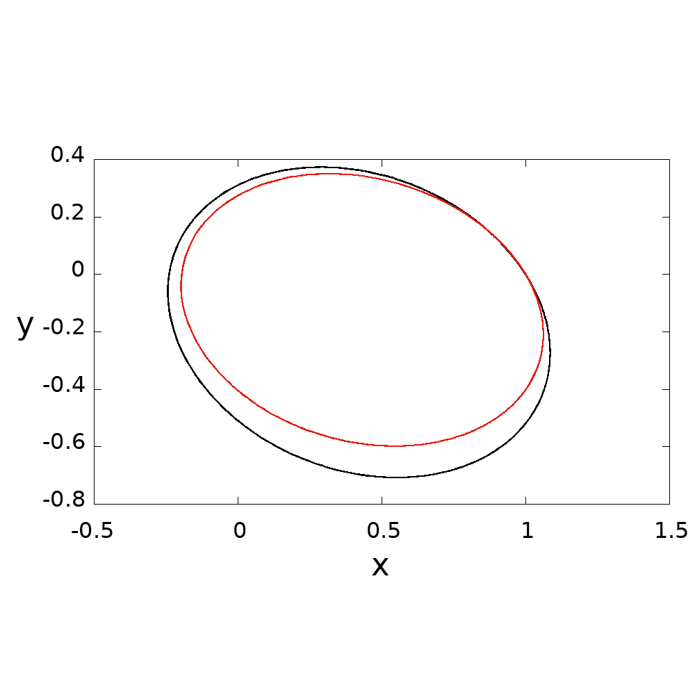
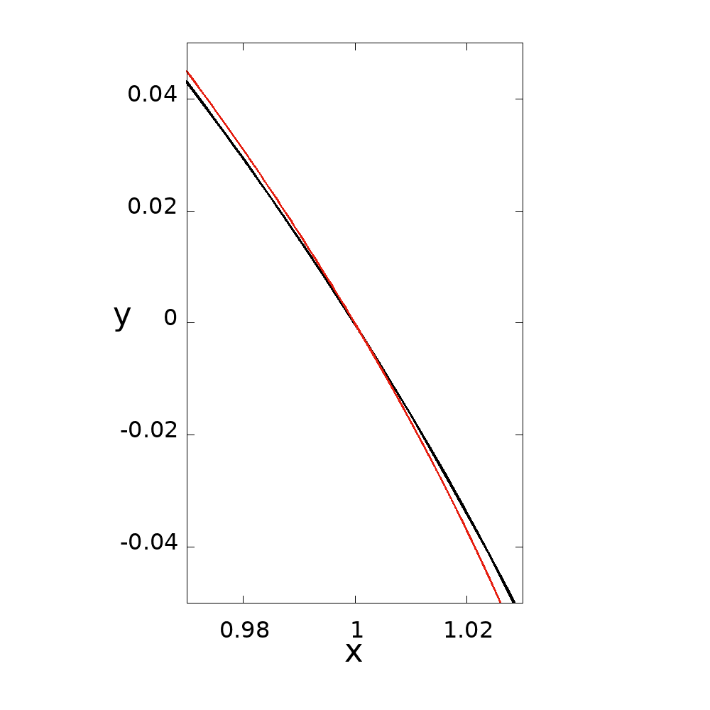
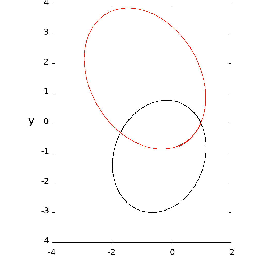
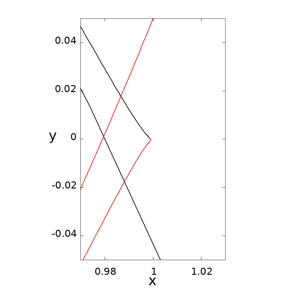
Figure 1: Representation on the inertial orbital plane $Oxy$ of orbits with a close encounter at $t=0$: the black curves represent the orbits computed for positive times, the red curves represent the same orbits computed for negative times. On the top panels we represent an orbit computed for $\mu=3\ 10^{-6}$ (close to the Sun-Earth mass ratio) for $E=-1.35$ and initial conditions $u_{1}(0)=-10^{-2}$, $u_{2}(0)=10^{-2}$, $U_{1}(0)=-4\ 10^{-6},U_{2}(0)=0.016243781387232425$; the close encounter determines a change of the semi-major axis of $\Delta a\sim 0.04349$ and $\Delta e\sim-0.07084$. On the bottom panels we represent an orbit computed for $\mu=10^{-3}$ (close to the Sun-Jupiter mass ratio) for $E=-1.35$ and initial conditions $u_{1}(0)=10^{-2}$, $u_{2}(0)=2\ 10^{-2}$, $U_{1}(0)=-2\ 10^{-5},U_{2}(0)=0.092703055510000729$; the close encounter determines a change of the semi-major axis of $\Delta a\sim-0.599$ and $\Delta e\sim-0.0708$. The right panels represent a zoom close to the secondary body $P_{2}$. Details about the numerical computation of these orbits and additional analysis are given in Section 5.

Let us give more details about the method of [19], which applies to the class of fast close encounters, i.e. the encounters occurring for values $E$ of the Hamilton function (1) satisfying:

$$3+2E-4\mu+\mu^{2}:=\alpha^{2}>0.$$ (2)

In [19], suitable resonant saddle-saddle Birkhoff normal forms of the Hamiltonian (1) represented with the Levi-Civita regularization had been considered. At this regard, we introduce the regularization of the Hamiltonian (1) following the method described in [20]: we first perform the phase-space translation:

$$X=x-x_{2}~{},\quad Y=y~{},\quad P_{X}=p_{x}~{},\quad P_{Y}=p_{y}-x_{2}~{}~{},$$ (3)

and then we introduce the Levi-Civita variables $u=(u_{1},u_{2})$, extended to the conjugate momenta $U=(U_{1},U_{2})$ and to the fictitious time $\tau$,

$$X=u_{1}^{2}-u_{2}^{2}~{},Y=2u_{1}u_{2}$$ (4)

$$P_{X}=\frac{U_{1}u_{1}-U_{2}u_{2}}{2|u|^{2}}~{},P_{Y}=\frac{U_{1}u_{2}+U_{2}u_{1}}{2|u|^{2}}$$ (5)

$$dt=|u|^{2}d\tau$$ (6)

where $|{u}|^{2}=u_{1}^{2}+u_{2}^{2}$. For any given value $E$ of the Hamiltonian (1), the Levi-Civita Hamiltonian:

$${\cal K}_{E}({u},{U})={1\over 8}\left(U_{1}+2|{u}|^{2}u_{2}\right)^{2}+{1\over 8}\left(U_{2}-2|{u}|^{2}u_{1}\right)^{2}-{1\over 2}|{u}|^{6}-\mu$$ (7)

$$-|{u}|^{2}\left(E+\frac{(1-\mu)^{2}}{2}\right)-(1-\mu)|{u}|^{2}\left[\frac{1}{\sqrt{1+2(u_{1}^{2}-u_{2}^{2})+|{u}|^{4}}}+u_{1}^{2}-u_{2}^{2}\right]$$ , (8)

is a regularization of the planar circular restricted three-body problem at $P_{2}$, in the sense that the solutions $(u(\tau),U(\tau))$ of the Hamilton equations of ${\cal K}_{E}$ satisfying ${\cal K}_{E}({u(0)},{U(0)})=0$ project, as long as $|u(\tau)|\neq 0$, on the solutions of the Hamilton equations of (1), up to the reparametrization of the time $t=t(\tau)$.

The Levi-Civita Hamiltonian (7) has an equilibrium point at $(u,U)=(0,0,0,0)$ which, as it was noticed in [19], is hyperbolic for values $E$ satisfying (2); in particular the Jacobian of the Hamiltonian vector field of (7) computed at the equilibrium has eigenvalues $\pm\alpha/2$ of multiplicity 2. This property has been exploited in the paper [19] by considering resonant hyperbolic Birkhoff normal forms (Bnf hereafter) of the regularized Hamiltonian. In [19], the Bnf have been introduced to discuss the application of Hartman’s theorem to the equilibrium point $(u,U)=(0,0,0,0)$; therefore no high order Bnf have been constructed, as it would be required by an high precision representation of the close encounters.

We recall that Birkhoff normal forms offer an highly effective method to approximate the solutions which are close to the equilibrium points of Hamiltonian systems. The method is useful also when the equilibrium is hyperbolic, since in this case it allows to study the stable/unstable manifolds, as well as the transits close to the equilibrium; for example, the method has been extensively used in the last decades to represent the solutions transiting close to the Lagrangian points $L_{1},L_{2}$ (see, for example, [32, 13, 15, 24, 6, 30, 26, 27, 28, 29, 31]). Depending on the resonant properties of Hamilton’s equations linearized at the equilibrium, a suitable normal form Hamiltonian of arbitrary order $N$ is conjugate to the original one, having the property that non-resonant monomials appear only at degrees larger than $N$. For the case at hand, with a standard procedure (which is recalled with all the details in Section 6), for any $N\geq 4$ we first define a canonical transformation:

$$(u,U)\rightarrow(q,p)$$

in a neighbourhood of $(u_{*},U_{*})=(0,0,0,0)$ (which is a fixed point of the transformation) conjugating the Levi-Civita Hamiltonian (7) to

$$K_{E}^{N}(q,p)=-\mu+{\alpha\over 2}(q_{1}p_{1}+q_{2}p_{2})+{\hat{K}}_{4}(q,p)+\ldots+{\hat{K}}_{N}(q,p)+{\cal R}_{N+2}(q,p)$$ (9)

where the Taylor series of ${\cal R}_{N+2}$ in $q,p$ starts with terms of degree at least $N+2$ and ${\hat{K}}_{j}$ are polynomials of degree $j$ in $q,p$ (only the polynomials with $j$ even number appear in the expansion) containing monomials:

$$c^{j,N}_{m,n}q_{1}^{m_{1}}q_{2}^{m_{2}}p_{1}^{n_{1}}p_{2}^{n_{2}}$$ (10)

with $m=(m_{1},m_{2}),n=(n_{1},n_{2})$ satisfying:

$$n_{1}+n_{2}=m_{1}+m_{2}.$$ (11)

Relation (11) is a direct consequence of the multiplicity of the characteristic multipliers, which qualifies the origin as ‘resonant’. We will call ‘non resonant’ the monomials (10) which do not satisfy relation (11); monomials which satisfy relation (11) will be called ‘integrable’ if $n_{1}=m_{1}$ and $n_{2}=m_{2}$, ‘resonant’ otherwise. The Hamilton function which is obtained by neglecting in $K_{E}^{N}(q,p)$ the reminder ${\cal R}_{N+2}(q,p)$:

$${\hat{K}}^{N}_{E}(q,p)=-\mu+{\alpha\over 2}(q_{1}p_{1}+q_{2}p_{2})+{\hat{K}}_{4}(q,p)+\ldots+{\hat{K}}^{N}(q,p)$$ (12)

will be called Bnf of order $N$. At variance with the full Hamiltonian (9), the Bnf (12) is Poisson commuting with the function $J(q,p)=q_{1}p_{1}+q_{2}p_{2}$ (this a direct consequence of property (11) of all the monomials of the normal form), and its Hamilton equations are integrable by quadratures. For example, by introducing the canonical variables $I_{j},\theta_{j}$ (defined for $I_{j}>0$; for $I_{j}<0$ obvious modifications are required):

$$q_{j}=\sqrt{I_{j}}e^{\theta_{j}}\ \ ,\ \ p_{j}=\sqrt{I_{j}}e^{-\theta_{j}}$$

the integrable monomials are conjugate to functions depending only on the actions $I_{j}$, while the resonant monomials are conjugate to functions depending on the actions $I_{j}$ and on multiples of $\theta_{1}-\theta_{2}$. As a consequence, the Hamiltonian flow is integrable by quadratures (see Section 2 for more details). Nevertheless, working out the explicit solutions for any order $N$ is cumbersome, because of the presence of the resonant terms (or equivalently, because of the dependence on $\theta_{1}-\theta_{2}$). The computation by quadratures may be particularly tricky to perform explicitly because the resonant terms depend on different powers of the action variables $I_{1},I_{2}$ and so the solution by quadratures requires to represent the roots of an algebraic polynomial in the action variables whose degree increases with the order $N$ of approximation. This is a minor problem if one is interested only in some low order approximation of the flow, but it poses a serious challenge if one needs a parametric representation of the flow which is valid for arbitrary (or for suitably large) order $N$. This problem does not exist for the Bnf of Hamiltonian systems with an the equilibrium point which, in the linear approximation, is not resonant (for example, this happens for equilibria which are linear elliptic with Diophantine frequencies). In fact, in this case the Birkhoff normal forms can be represented with a function depending only on action variables, whose flow is easily represented.

In this paper, we obtain a major improvement in the computation of the solutions of the flow of the Bnf (12). Precisely, after proving a remarkable factorization property of Hamiltonians (12) for all $N$, we are able to give its Hamilton equations a different Hamiltonian representation, where the origin $(u,U)=(0,0,0,0)$ is a non-resonant focus-focus equilibrium point. As a consequence, we are able to perform an additional sequence of focus-focus Birkhoff normalizations conjugating the Hamiltonian to a normal form depending only on the action variables. Thus, we obtain a considerable simplification in the computation of close encounters, which is valid for small values of the mass parameter $\mu$. The factorization property that we prove for the Bnf is the following: for all $N$ the Birkhoff normal forms (12) are divided by the polynomial $J(q,p)=q_{1}p_{1}+q_{2}p_{2}$, i.e. they are represented in the form:

$$\hat{K}^{N}_{E}(q,p)=-\mu+(q_{1}p_{1}+q_{2}p_{2})\left({\alpha\over 2}+k_{2}(q,p)+\ldots+k_{N-2}(q,p)\right),$$ (13)

where $k_{j}(q,p)$ are polynomials of degree $j$. Since both functions $J(q,p)$ and $k(q,p)={\alpha\over 2}+k_{2}(q,p)+\ldots+k_{N-2}(q,p)$ are first integrals for the Birkhoff normal form $\hat{K}^{N}_{E}$, the solutions of Hamilton’s equations with initial data satisfying

$$k(q(0),p(0)):=\kappa\ \ \ \ ,\ \ \ \ J(q(0),p(0)):=\eta\ \ ,$$

with $\kappa\eta=\mu$, satisfy the Hamilton equations of:

$${\cal H}(q,p)=\kappa(q_{1}p_{1}+q_{2}p_{2})+\eta(k_{2}(q,p)+k_{4}(q,p)+\ldots+k_{N-2}(q,p)).$$ (14)

Since $\eta$ is hereafter treated as a parameter, the terms $J(q,p)k_{j}(q,p)$ (which in the Hamiltonian (13) are polynomials of degree $j+2$), are transformed into polynomials $\eta k_{j}(q,p)$ which have degree $j$; in particular $\eta k_{2}(q,p)$ has degree $2$ and modifies the linearization of the Hamiltonian vector field at $(q,p)=(0,0,0,0)$. Therefore, we have the opportunity to construct a different Bnf for Hamiltonian (14) depending on this new linearization.

For initial conditions satisfying $\hat{K}^{N}_{E}(q,p)=0$ we have $\eta\neq 0$, we therefore proceed by considering the case $\eta\neq 0$. By representing explicitly the term $k_{2}(q,p)$, we notice that Hamiltonian (14) has the representation:

$${\cal H}(q,p)=\sum_{j\geq 1}^{N-2\over 2}h_{2j}(q,p)$$

with quadratic part:

$$h_{2}=\kappa(q_{1}p_{1}+q_{2}p_{2})+\eta k_{2}(q,p)=\Lambda(q_{1}p_{1}+q_{2}p_{2})+\Omega(p_{2}q_{1}-p_{1}q_{2})$$

with $\Lambda=\kappa$ and $\Omega=\eta/(4\alpha)$, while for $j\geq 2$ we have: $h_{2j}(q,p)=\eta k_{2j}(q,p)$. The origin $(q,p)=(0,0,0,0)$ is an equilibrium point, with characteristic exponents:

$$\pm\Omega\pm i\Lambda,$$

so that the equilibrium is focus-focus with eigenvalues of multiplicity 1. Therefore, we can proceed by defining a second sequence of Birkhoff normalizations of ${\cal H}$ using the focus-focus character of $(q,p)=(0,0,0,0)$. It is important to remark that the functions generating these Birkhoff normalizations have small divisors proportional to $\eta$, which may be very small. However, this does not produce divergence of the norms since, by the factorization property, the polynomial terms of order larger than 4 of the Bnf are proportional to $\eta$ as well, so that the generating functions of Birkhoff normalizations are not singular at $\eta=0$. Moreover, the generating functions depend in straightforward way on the parameters $\Lambda,\Omega$ (see Section 4 for details), so that the two additional parameters do not introduce any substantial complexity in the symbolic computation of the normal forms.

We therefore show that Hamiltonian (14) is conjugate by a (complex) canonical transformation:

$$(q,p)\mapsto(Q,P)$$

defined in a neighbourhood of $(q,p)=(0,0,0,0)$ (which is a fixed point of the transformation) to the focus-focus Bnf:

$$H^{N}_{E}(Q,P)=(i\Omega-\Lambda)Q_{1}P_{1}-(i\Omega+\Lambda)Q_{2}P_{2}+{\hat{h}}(Q_{1}P_{1},Q_{2}P_{2})+{\cal R}_{N}(Q,P)$$ (15)

where ${\hat{h}}(I_{1},I_{2})$ is a polynomial in $I_{1},I_{2}$ containing monomials of degree ranging between $2$ and $(N-2)/2$, and the remainde ${\cal R}_{N}(Q,P)$ is a series which starts with terms of degree $N$. By neglecting the remainder we obtain the integrable Hamiltonian:

$${\hat{H}}^{N}_{E}(Q,P)=(i\Omega-\Lambda)Q_{1}P_{1}-(i\Omega+\Lambda)Q_{2}P_{2}+{\hat{h}}(Q_{1}P_{1},Q_{2}P_{2})$$ (16)

whose flow is represented explicitly by the same formulas, independently on $N$, since the functions $I_{1}=Q_{1}P_{1},I_{2}=Q_{2}P_{2}$ are first integrals:

$$Q_{j}(\tau)=Q_{j}(0)e^{\hat{\kappa}_{j}\tau}\ \ ,\ \ P_{j}(t)=P_{j}(0)e^{-\hat{\kappa}_{j}\tau}\ \ ,\ \ j=1,2$$ (17)

where:

$$\hat{\kappa}_{j}={\partial\ \over\partial I_{j}}\left((i\Omega-\Lambda)I_{1}-(i\Omega+\Lambda)I_{2}+{\hat{h}}(I_{1},I_{2})\right)_{|_{I_{1}=I_{1}(0),I_{2}=I_{2}(0)}}.$$

For each order of approximation, all the Birkhoff normalizations and the parameters of the focus-focus dynamics (17) are represented by polynomials whose coefficients can be computed iteratively with a computer algebra system (see Sections 6 and 5).

Remarks. (I) Parametric representations of close encounters may be used to implement a numerical integrator of the close encounters by explicitly representing with a computer program the flow of the Bnf $K^{N}_{E}(q,p)$.

(II) The parametric representations of the solutions offered by the Bnf are approximate, because they are obtained by neglecting the remainders ${\cal R}_{N}(q,p)$, which are polynomials in the $(q,p)$ variables of order $N$. Therefore, the distance of $(q,p)$ from the equilibrium point $(0,0,0,0)$ is the small parameter of the problem. We recall that the normal form variables $q,p$ are obtained from the composition of a linear transformation of the Levi-Civita variables $(u,U)$ with the Birkhoff normalizations. During a transit in a ball of radius $\sigma$ centered at $P_{2}$, we have $|u|^{2}<\sigma$ (which becomes $0$ at collision); but also $|U|$ remains small (with limit value proportional to $\sqrt{\mu}$ at collision).

(III) As it is typical of normal form Hamiltonians, and also of numerical integrators of given order, the remainder ${\cal R}_{N}(q,p)$ may depend on $N$ in a non-trivial case, so that the increment of $N$ may produce an improvement only up to a finite large value. For the numerical examples of Section 5, obtained for the large order $N=30$, we see that we would still have the opportunity to reduce the error of the parametric representation by considering also larger values of $N$.

The paper is organized as follows: in Section 2 we describe the properties of the first sequence of saddle-saddle Bnf; in Section 3 we prove that all the Birkhoff normal forms presented in Section 2 are divided by $q_{1}p_{1}+q_{2}p_{2}$; in Section 4 we provide all the details needed to construct the second sequence of focus-focus Bnf, and the solution of its Hamilton equations; in Section 5 we provide some numerical demonstrations of the method for values of the mass parameter representative of the Sun-Earth and the Sun-Jupiter cases; in the Appendix 1 (Section 6) we present the technical details of the construction of the Birkhoff normal forms for 2-degrees of freedom Hamiltonian systems; in the Appendix 2 (Section 7) we provide the generating functions which define the Bnf of order $N=6$; Conclusions and Perspectives are provided in Section 8.

2 The resonant saddle-saddle Birkhoff normal form

We expand the Levi-Civita Hamiltonian (7) as a Taylor series of the variables $u,U$:

$${\cal K}_{E}=-\mu+{\cal K}_{2}(u,U;E)+{\cal K}_{4}(u,U)+\sum_{j\geq 3}{\cal K}_{2j}(u)$$

where:

$${\cal K}_{2}={1\over 8}(U_{1}^{2}+U_{2}^{2})-{1\over 2}\left(3+2E-4\mu+\mu^{2}\right)(u_{1}^{2}+u_{2}^{2})={1\over 8}(U_{1}^{2}+U_{2}^{2})-{\alpha^{2}\over 2}(u_{1}^{2}+u_{2}^{2}),$$

$${\cal K}_{4}={1\over 2}(u_{1}^{2}+u_{2}^{2})(U_{1}u_{2}-U_{2}u_{1}),$$

and, for all $j\geq 3$,

$${\cal K}_{2j}=-(1-\mu)\ T_{2j}\left[|{u}|^{2}\left(\frac{1}{\sqrt{1+2(u_{1}^{2}-u_{2}^{2})+|{u}|^{4}}}\right)\right]$$ (18)

where $T_{k}f(u,U)$ denotes the Taylor term of degree $k$ of a function $f(u,U)$. For $E$ satisfying

$$\alpha^{2}=3+2E-4\mu+\mu^{2}>0$$

the origin is an hyperbolic equilibrium point with real eigenvalues $\pm{\alpha/2}$ of multiplicity 2. Therefore, we introduce hyperbolic variables by means of the canonical transformation:

$$(q_{1},q_{2},p_{1},p_{2})=C^{-1}(u_{1},u_{2},U_{1},U_{2})$$ (19)

where $C$ is the real matrix:

$$C=\left(\begin{array}[]{cccc}\frac{1}{2\sqrt{\alpha}}&0&-\frac{1}{2\sqrt{\alpha}}&0\\ 0&\frac{1}{2\sqrt{\alpha}}&0&-\frac{1}{2\sqrt{\alpha}}\\ \sqrt{\alpha}&0&\sqrt{\alpha}&0\\ 0&\sqrt{\alpha}&0&\sqrt{\alpha}\\ \end{array}\right).$$

The transformation (19) conjugates the Hamiltonian ${\cal K}_{E}$ to:

$$K_{E}(q,p)=-\mu+\sum_{j\geq 1}K_{2j}(q,p)$$ (20)

with:

$$K_{2}={\alpha\over 2}(q_{1}p_{1}+q_{2}p_{2})$$

and, for all $j$, we introduce the representation:

$$K_{2j}=\sum_{m,n\in{\mathbb{N}}^{2}:|m|+|n|=2j}c_{m,n}q^{m}p^{n},$$

where $m=(m_{1},m_{2}),n=(n_{1},n_{2})$ are multi-indices and, following standard notation for multi-indices, for any multi-index $\nu\in{\mathbb{Z}}^{2}$, we denote $|\nu|=\nu_{1}+\nu_{2}$.

The Hamiltonian $K_{E}$ is given the Birkhoff normal form by a canonical transformation ${\cal C}_{N}$, defined in a neighbourhood of $(q_{*},p_{*})=(0,0,0,0)$ (which is a fixed point of the transformation) conjugating $K_{E}$ to:

$$K_{E}^{N}(q,p)=-\mu+{\alpha\over 2}(q_{1}p_{1}+q_{2}p_{2})+{\hat{K}}_{4}(q,p)+\ldots+{\hat{K}}_{N}(q,p)+{\cal R}_{N+2}(q,p)$$ (21)

where the Taylor series of ${\cal R}_{N+2}$ in $q,p$ starts with terms of order at least $N+2$ and ${\hat{K}}_{j}$ are polynomials of order $j$ in $q,p$ (only the polynomials with $j$ even number appear in the expansion) containing monomials:

$$c^{j,N}_{m,n}q_{1}^{m_{1}}q_{2}^{m_{2}}p_{1}^{n_{1}}p_{2}^{n_{2}}$$ (22)

with $m=(m_{1},m_{2}),n=(n_{1},n_{2})$ satisfying:

$$n_{1}+n_{2}=m_{1}+m_{2}.$$ (23)

The definition of the canonical transformation is defined following a standard procedure, which we describe in detail in the Appendix 1 (Section 6).

Remark. The standard procedure which is described in Section 6 is applied by setting the parameters $\lambda_{1},\lambda_{2}=\alpha/2$, so that the divisors entering the definition of the generating functions (69):

$$\lambda_{1}(n_{1}-m_{1})+\lambda_{2}(n_{2}-m_{2})=(\alpha/2)(n_{1}+n_{2}-m_{1}-m_{2}),$$

are proportional to the integer $n_{1}+n_{2}-m_{1}-m_{2}$. As a consequence, the resonant relation (62) becomes the relation (23).

We consider the Hamiltonian which is obtained by neglecting the remainder ${\cal R}_{N+2}(q,p)$ in $K^{N}_{E}(q,p)$:

$${\hat{K}}^{N}_{E}(q,p)=-\mu+{\alpha\over 2}(q_{1}p_{1}+q_{2}p_{2})+{\hat{K}}_{4}(q,p)+\ldots+{\hat{K}}^{N}(q,p),$$

which will be called Bnf of order $N$. For example, at order $N=6$ we have:

$$\hat{K}^{6}_{E}(q,p)=-\mu+{\alpha\over 2}(q_{1}p_{1}+q_{2}p_{2})-{1\over 4\alpha}(p_{1}q_{2}-p_{2}q_{1})(q_{1}p_{1}+q_{2}p_{2})$$ (24)

$$-{(p_{1}q_{1}+p_{2}q_{2})\over 16\alpha^{3}}\Big{[}-5(1-\mu)(q^{2}_{1}p^{2}_{1}+q^{2}_{2}p^{2}_{2})+2p_{1}p_{2}q_{1}q_{2}(6-7\mu)$$ (25)

$$+(q^{2}_{1}p^{2}_{2}+q^{2}_{2}p^{2}_{1})(4-3\mu)\Big{]}.$$ (26)

Higher order Bnf can be computed using modern computer algebra systems, with a symbolic representation of the coefficients of all their monomials as a function of the parameters $\mu,E$.

The Bnf of any order $N$ has the first integrals ${\hat{K}}^{N}_{E}(q,p)$ and $J(q,p)=q_{1}p_{1}+q_{2}p_{2}$ (this a direct consequence of relation (11) of all the monomials of the normal form), and is integrable by quadratures. In fact, by introducing the canonical variables $I_{j},\theta_{j}$ (defined for $I_{j}>0$; for $I_{j}<0$ obvious modifications are required):

$$q_{j}=\sqrt{I_{j}}e^{\theta_{j}}\ \ ,\ \ p_{j}=\sqrt{I_{j}}e^{-\theta_{j}}$$

the monomials of ${\hat{K}}^{N}_{E}$ are conjugate to:

$$\sqrt{I_{1}}^{m_{1}+n_{1}}\sqrt{I_{2}}^{m_{2}+n_{2}}e^{(m_{1}-n_{1})\theta_{1}}e^{(m_{2}-n_{2})\theta_{2}}=\sqrt{I_{1}}^{m_{1}+n_{1}}\sqrt{I_{2}}^{m_{2}+n_{2}}e^{(m_{1}-n_{1})(\theta_{1}-\theta_{2})},$$

where the last equality follows from relation (11). With a further change to the action-angle variables $\hat{I}_{1},\hat{I}_{2},\hat{\theta}_{1},\hat{\theta}_{2}$:

$$\hat{I}_{1}=I_{1}\ \ ,\ \ \hat{I}_{2}=I_{1}+I_{2}\ \ ,\ \ \hat{\theta}_{1}=\theta_{1}-\theta_{2}\ \ ,\ \ \hat{\theta}_{2}=\theta_{2}$$

the Bnf is finally conjugate to an Hamiltonian $h^{N}_{E}(\hat{I}_{1},\hat{I}_{2},\hat{\theta}_{1})$ which is independent on $\hat{\theta}_{2}$, and therefore for any value of the first integral $\hat{I}_{2}=J(q,p)$ can be studied as a reduced 1-degree of freedom Hamiltonian system. Nevertheless, working out the explicit solutions for its Hamilton equations by quadratures, which in particular requires to find the solutions of the equation:

$$h^{N}_{E}(\hat{I}_{1},\hat{I}_{2},\hat{\theta}_{1})=0$$ (27)

in the form $\hat{I}_{1}:=\hat{I}_{1}(\hat{I}_{2},\hat{\theta}_{1})$ for any $N$, is cumbersome.

3 A remarkable property of the Birkhoff normal forms

3.1 A permutation symmetry

We say that the polynomial $F(q,p)$ of the hyperbolic variables $q,p$:

$$F(q,p):=\sum_{\ell=1}^{L}\ \ \sum_{m,n:\ |m|+|n|=2\ell}c_{m,n}q^{m}p^{n}$$ (28)

has the permutation symmetry if for each multi-index $m,n=m_{1},m_{2},n_{1},n_{2}$ we have:

$$c_{m,n}=(-1)^{\sigma_{m,n}+{|m|+|n|-2\over 2}}c_{\overline{m,n}}\ \ ,$$ (29)

where $\overline{{m,n}}=n_{2},n_{1},m_{2},m_{1}$ and $\sigma_{m,n}=1$ is $m_{1}+n_{1}$ is odd, $\sigma_{m,n}=0$ otherwise.

We denote by $\Pi F$ the expansion obtained by summing all the resonant terms of $F$:

$$\Pi F:=\sum_{\ell=1}^{L}\ \ \sum_{|m|+|n|=2\ell,m_{1}+m_{2}=n_{1}+n_{2}}c_{m,n}q^{m}p^{n}.$$

We show that for any polynomial $F(q,p)$ satisfying the permutation symmetry, $\Pi F$ is divisible by $q_{1}p_{1}+q_{2}p_{2}$. First, from the property (29) we have:

• $c_{m_{1},m_{2},m_{2},m_{1}}=0$ for any $m_{1},m_{2}$ with $m_{1}+m_{2}\geq 1$. In fact, for $n_{1}=m_{2},n_{2}=m_{1}$, Eq. (29) becomes:

  $$c_{m_{1},m_{2},m_{2},m_{1}}=(-1)^{\sigma_{m,n}}(-1)^{m_{1}+m_{2}-1}c_{m_{1},m_{2},m_{2},m_{1}}.$$

  If $m_{1}+n_{1}=m_{1}+m_{2}$ is even, then $(-1)^{\sigma_{m,n}}=1$ and $(-1)^{m_{1}+m_{2}}=1$; if $m_{1}+n_{1}=m_{1}+m_{2}$ is odd, then $(-1)^{\sigma_{m,n}}=-1$ and $(-1)^{m_{1}+m_{2}}=-1$. In both cases we have $(-1)^{\sigma_{m,n}+{|m|+|n|-2\over 2}}=(-1)^{\sigma_{m,n}}(-1)^{m_{1}+m_{2}-1}=-1$, from which it follows $c_{m_{1},m_{2},m_{2},m_{1}}=0$.

• Consider any $m,n$ with $n_{1},n_{2}\neq m_{2},m_{1}$ and $m_{1}+m_{2}=n_{1}+n_{2}$. The two coefficients $c_{m,n},c_{\overline{m.n}}$ satisfy:

  $$c_{m,n}(-1)^{m_{1}}+c_{\overline{m,n}}(-1)^{n_{2}}=0.$$ (30)

  In fact, since $m_{1}+m_{2}=n_{1}+n_{2}$ we rewrite Eq. (29) as:

  $$c_{m,n}=-(-1)^{\sigma_{m,n}}(-1)^{m_{1}+m_{2}}c_{\overline{m,n}}.$$

  If $m_{1}+n_{1},m_{2}+n_{2}$ are both even, on the one hand we have $(-1)^{\sigma_{m,n}}=1$ so that:

  $$c_{m,n}=-(-1)^{m_{1}+m_{2}}c_{\overline{m,n}},$$

  as well as:

  $$c_{m,n}(-1)^{m_{1}}+c_{\overline{m,n}}(-1)^{m_{2}}=0.$$

  On the other hand, since $m_{2}+n_{2}$ is even, we have $(-1)^{m_{2}}=(-1)^{-n_{2}}=(-1)^{n_{2}}$, and so we obtain (30). If instead $m_{1}+n_{1},m_{2}+n_{2}$ are both odd, we have:

  $$c_{m,n}=(-1)^{m_{1}+m_{2}}c_{\overline{m,n}},$$

  as well as:

  $$c_{m,n}(-1)^{m_{1}}-c_{\overline{m,n}}(-1)^{m_{2}}=0.$$

  Since $m_{2}+n_{2}$ is odd, we have $(-1)^{m_{2}}=-(-1)^{-n_{2}}=-(-1)^{n_{2}}$, and so we obtain (30).

From (i) and (ii) it follows that we can represent $\Pi F$ in the form:

$$\Pi F(q,p)=(q_{1}p_{1}+q_{2}p_{2})(c+f_{2}(q,p)+\ldots+f_{N-2}(q,p))$$

where $f_{j}(q,p)$ are polynomials of degree $j$ in the variables $q,p$.

In fact, in $\Pi F(q,p)$ we have all the monomials of $F$ corresponding to $m,n$ with $m_{1}+m_{2}=n_{1}+n_{2}$. If $m,n=\overline{m,n}$, from (i) we have $c_{m,n}=0$. If $m,n\neq\overline{m,n}$ we consider the sum of the symmetric terms:

$$S_{m,n}=c_{m,n}q_{1}^{m_{1}}q_{2}^{m_{2}}p_{1}^{n_{1}}p_{2}^{n_{2}}+c_{\overline{m,n}}q_{1}^{n_{2}}q_{2}^{n_{1}}p_{1}^{m_{2}}p_{2}^{m_{1}},$$ (31)

and prove that $S_{m,n}$ is divided by $q_{1}p_{1}+q_{2}p_{2}$. Necessary condition for a polynomial $S(q_{1},q_{2},p_{1},p_{2})$ to be divisible by $(q_{1}p_{1}+q_{2}p_{2})$ is that the rational function ${\cal S}=S(-q_{2}p_{2}/p_{1},q_{2},p_{1},p_{2})$ is identically zero. Since the ring of polynomials of four variables has unique factorization (see [14], pages 153, 154), the condition is also sufficient. Let us therefore consider the rational function:

$${\cal S}_{m,n} = S_{m,n}(-q_{2}p_{2}/p_{1},q_{2},p_{1},p_{2})$$

$$= c_{m,n}(-1)^{m_{1}}q_{2}^{m_{2}+m_{1}}p_{1}^{n_{1}-m_{1}}p_{2}^{n_{2}+m_{1}}+c_{\overline{m,n}}(-1)^{n_{2}}q_{2}^{n_{1}+n_{2}}p_{1}^{m_{2}-n_{2}}p_{2}^{m_{1}+n_{2}}.$$

Since the monomials of $\Pi F$ satisfy $m_{1}+m_{2}=n_{1}+n_{2}$, the powers of $q_{2},p_{1},p_{2}$ are the same for both terms appearing in ${\cal S}_{m,n}$, and therefore we have:

$${\cal S}_{m,n}=\left(c_{m,n}(-1)^{m_{1}}+c_{\overline{m,n}}(-1)^{n_{2}}\right)q_{2}^{m_{2}+m_{1}}p_{1}^{n_{1}-m_{1}}p_{2}^{n_{2}+m_{1}}.$$

By property (ii) the rational function ${\cal S}_{m,n}$ vanishes identically, and therefore the polynomial $S_{m,n}$ in (31) is divided by $q_{1}p_{1}+q_{2}p_{2}$. Since $\Pi F$ is the sum of polynomials (31), it is divided by $q_{1}p_{1}+q_{2}p_{2}$ as well.

3.2 The Levi-Civita Hamiltonian has the permutation symmetry

In this Subsection we prove that any finite order truncation of the Levi-Civita Hamiltonian represented with the hyperbolic variables $q,p$, i.e. Hamiltonian (20), has the permutation symmetry. First, one directly checks that the terms:

$$K_{2}={\alpha\over 2}(q_{1}p_{1}+q_{2}p_{2})$$

$$K_{4}=\Big{(}-\frac{{q_{1}}{p_{1}}^{2}{p_{2}}}{8\alpha}-\frac{{q_{1}}{q_{2}}^{2}{p_{2}}}{8\alpha}\Big{)}+\Big{(}-\frac{{q_{1}}{q_{2}}{p_{1}}^{2}}{4\alpha}-\frac{{q_{2}}^{2}{p_{1}}{p_{2}}}{4\alpha}\Big{)}+\Big{(}\frac{{q_{2}}{p_{1}}^{3}}{8\alpha}+\frac{{q_{2}}^{3}{p_{1}}}{8\alpha}\Big{)}+$$

$$+\Big{(}\frac{{q_{2}}{p_{1}}{p_{2}}^{2}}{8\alpha}+\frac{{q_{1}}^{2}{q_{2}}{p_{1}}}{8\alpha}\Big{)}+\Big{(}\frac{{q_{1}}^{2}{p_{1}}{p_{2}}}{4\alpha}+\frac{{q_{1}}{q_{2}}{p_{2}}^{2}}{4\alpha}\Big{)}+\Big{(}-\frac{{q_{1}}{p_{2}}^{3}}{8\alpha}-\frac{{q_{1}}^{3}{p_{2}}}{8\alpha}\Big{)}$$

have the permutation symmetry (the symmetric terms have been grouped together; for all the terms of $K_{4}$ we have $\sigma_{m,n}=1$ and $|m|+|n|=4$, so that (29) becomes $c_{mn}=c_{\overline{m,n}}$).

To prove the property for all the other terms $K_{2j}$ with $j\geq 3$, we introduce the parametric function:

$${\cal K}^{\geq 6}(u;\lambda)=-\sum_{\ell\geq 3}(1-\mu)\ T_{2\ell}\left[|{u}|^{2}\left(\frac{1}{\sqrt{1+2\lambda(u_{1}^{2}-u_{2}^{2})+\lambda^{2}|{u}|^{4}}}\right)\right]$$

and the Taylor expansion:

$${\cal K}^{\geq 6}(u;\lambda):=\sum_{j\geq 2}\lambda^{j}{\cal P}_{j}(u),\hfill$$

where ${\cal P}_{j}(u)$ is a polynomial in the variables $u$ of degree $2j+2$; for $\lambda=1$ we have:

$${\cal K}_{E}(u,U)=-\mu+{\cal K}_{2}(u,U)+{\cal K}_{4}(u,U)+{\cal K}^{\geq 6}(u;1).$$

The composition of the functions ${\cal K}^{\geq 6}$ and ${\cal P}_{j}$ with the canonical transformation:

$$(u,U)=C(q,p)$$

provides the functions $K^{\geq 6},P_{j}$:

$$K^{\geq 6}(q,p;\lambda)=\sum_{j\geq 2}\lambda^{j}P_{j}(q,p)$$

with $P_{j}(q,p)=K_{2j+2}(q,p)$ for all $j\geq 2$.

For any $(q,p)$, by denoting with $(u,U):=C(q,p)$, $(\tilde{q}_{1},\tilde{q}_{2},\tilde{p}_{1},\tilde{p}_{2}):=(p_{2},p_{1},q_{2},q_{1})$ and $(\tilde{u},\tilde{U}):=C(\tilde{q},\tilde{p})$, we have $(\tilde{u},\tilde{U})=(-u_{2},-u_{1},U_{2},U_{1})$ as well as:

$${\cal K}^{\geq 6}(\tilde{u};-\lambda)={\cal K}^{\geq 6}(u;\lambda),$$

and consequently:

$$\sum_{j\geq 2}\lambda^{j}{\cal P}_{j}(u)=\sum_{j\geq 2}\lambda^{j}(-1)^{j}{\cal P}_{j}(\tilde{u})\ \ .$$

By identifying the coefficients of the two Taylor expansions in $\lambda$ at both sides of the last equation, we obtain:

$${\cal P}_{j}(u)=(-1)^{j}{\cal P}_{j}(\tilde{u}),$$ (32)

as well as:

$$P_{j}(q,p)=(-1)^{j}P_{j}(p_{2},p_{1},q_{2},q_{1}).$$ (33)

From:

$$P_{j}=\sum_{m,n:|m|+|n|=2j+2}c_{m,n}q^{m}p^{n},$$

by equating the coefficients of the same term $q^{m}p^{n}$ from both sides of equality (33) we obtain:

$$c_{m,n}=(-1)^{j}c_{\overline{m,n}}=(-1)^{|m|+|n|-2\over 2}c_{\overline{m,n}}\ \ .$$ (34)

Since the polynomials ${\cal P}_{j}$ depend on the $u$ only through $u_{1}^{2},u_{2}^{2}$, in the corresponding polynomial $P_{j}(q,p)=K_{2j+2}(q,p)$ there are only monomials $c_{m,n}q^{m}p^{n}$ where $m_{1}+n_{1},m_{2}+n_{2}$ are even numbers, and so $\sigma_{m,n}=0$. Therefore, eq. (34) can be rewritten as:

$$c_{m,n}=(-1)^{\sigma_{m,n}+{|m|+|n|-2\over 2}}c_{\overline{m,n}},$$ (35)

as it is required by (29). Therefore we have proved that all finite truncations of $K(q,p)$ have the permutation symmetry.

3.3 The Birkhoff normal forms of the Levi-Civita Hamiltonian have the permutation symmetry

In this Subsection prove that the Bnf (12) of arbitrary order $N$ have the permutation symmetry, and therefore are divisible by $q_{1}p_{1}+q_{2}p_{2}$.

Consider any couple of functions:

$$F=\sum_{j\geq 1}\sum_{|m|+|n|=2j}c_{m,n}q^{m}p^{n}$$

$$\tilde{F}=\sum_{j\geq 1}\sum_{|m|+|n|=2j}\tilde{c}_{m,n}q^{m}p^{n}$$

having the permutation symmetry, and the generating function:

$$\chi_{{}_{2i}}=\sum_{|m|+|n|=2i,|m|\neq|n|}{c_{m,n}\over{\alpha\over 2}(|m|-|n|)}q^{m}p^{n}$$

which is constructed from the coefficients of the monomials of degree $2i$ of the function $F$. We prove that $\{\tilde{F},\chi_{{}_{2i}}\}$ has the permutation symmetry. It is sufficient to prove that, for any $j\geq 1$, by considering:

$$\tilde{F}_{2j}=\sum_{|\tilde{m}|+|\tilde{n}|=2j}\tilde{c}_{\tilde{m},\tilde{n}}q^{\tilde{m}}p^{\tilde{n}},$$

the function $\{\tilde{F}_{2j},\chi_{{}_{2i}}\}$ has the permutation symmetry.

We have:

$$\{\tilde{F}_{2j},\chi_{{}_{2i}}\} =\sum_{|m|+|n|=2i,|m|\neq|n|}\ \ \sum_{|\tilde{m}|+|\tilde{n}|=2j}\ \ {\tilde{c}_{\tilde{m},\tilde{n}}c_{m,n}\over{\alpha\over 2}(|m|-|n|)}\times$$ (36)

$$\times\Big{[}(\tilde{m}_{1}n_{1}-m_{1}\tilde{n}_{1})q_{1}^{m_{1}+\tilde{m}_{1}-1}q_{2}^{m_{2}+\tilde{m}_{2}}p_{1}^{n_{1}+\tilde{n}_{1}-1}p_{2}^{n_{2}+\tilde{n}_{2}}$$ (37)

$$+(\tilde{m}_{2}n_{2}-m_{2}\tilde{n}_{2})q_{1}^{m_{1}+\tilde{m}_{1}}q_{2}^{m_{2}+\tilde{m}_{2}-1}p_{1}^{n_{1}+\tilde{n}_{1}}p_{2}^{n_{2}+\tilde{n}_{2}-1}\Big{]}$$ (38)

$$:=\sum_{|m|+|n|=2i,|m|\neq|n|}\ \ \sum_{|\tilde{m}|+|\tilde{n}|=2j}\Big{[}{\cal P}_{m,n,\tilde{m},\tilde{n}}+{\cal Q}_{m,n,\tilde{m},\tilde{n}}\Big{]}\ \$$ (39)

where:

$${\cal P}_{m,n,\tilde{m},\tilde{n}}:={\tilde{c}_{\tilde{m},\tilde{n}}c_{m,n}\over{\alpha\over 2}(|m|-|n|)}(\tilde{m}_{1}n_{1}-m_{1}\tilde{n}_{1})q_{1}^{m_{1}+\tilde{m}_{1}-1}\ q_{2}^{m_{2}+\tilde{m}_{2}}p_{1}^{n_{1}+\tilde{n}_{1}-1}p_{2}^{n_{2}+\tilde{n}_{2}}$$

$${\cal Q}_{m,n,\tilde{m},\tilde{n}}:={\tilde{c}_{\tilde{m},\tilde{n}}c_{m,n}\over{\alpha\over 2}(|m|-|n|)}(\tilde{m}_{2}n_{2}-m_{2}\tilde{n}_{2})\ q_{1}^{m_{1}+\tilde{m}_{1}}q_{2}^{m_{2}+\tilde{m}_{2}-1}p_{1}^{n_{1}+\tilde{n}_{1}}p_{2}^{n_{2}+\tilde{n}_{2}-1}.$$

The double sum in (39) can be rearranged as the sum of couples of symmetric monomials ${\cal P}_{m,n,\tilde{m},\tilde{n}}:=\xi q_{1}^{M_{1}}q_{2}^{M_{2}}p_{1}^{N_{1}}p_{2}^{N_{2}}$ and ${\cal Q}_{\overline{m,n},\overline{\tilde{m},\tilde{n}}}:=\eta q_{1}^{N_{2}}q_{2}^{N_{1}}p_{1}^{M_{2}}p_{2}^{M_{1}}$ satisfying:

$$\xi=(-1)^{\sigma_{M,N}+{|M|+|N|-2\over 2}}\eta,$$ (40)

which implies that $\{\tilde{F}_{j},\chi_{{}_{2i}}\}$ has the permutation symmetry.

In fact, consider $m,n,\tilde{m},\tilde{n}$ such that $m,n\neq\overline{m,n}$ and $\tilde{m},\tilde{n}\neq\overline{\tilde{m},\tilde{n}}$ (otherwise $\tilde{c}_{\tilde{m},\tilde{n}}c_{m,n}=0$ and there is nothing more to prove), and the term:

$${\cal P}_{m,n,\tilde{m},\tilde{n}} := {\tilde{c}_{\tilde{m},\tilde{n}}c_{m,n}\over{\alpha\over 2}(|m|-|n|)}(\tilde{m}_{1}n_{1}-m_{1}\tilde{n}_{1})q_{1}^{m_{1}+\tilde{m}_{1}-1}\ q_{2}^{m_{2}+\tilde{m}_{2}}p_{1}^{n_{1}+\tilde{n}_{1}-1}p_{2}^{n_{2}+\tilde{n}_{2}}$$ (41)

$$= \xi q_{1}^{M_{1}}q_{2}^{M_{2}}p_{1}^{N_{1}}p_{2}^{N_{2}}$$ (42)

where we denote:

$$M_{1}=m_{1}+\tilde{m}_{1}-1,M_{2}=m_{2}+\tilde{m}_{2},N_{1}=n_{1}+\tilde{n}_{1}-1,N_{2}=n_{2}+\tilde{n}_{2}.$$ (43)

and:

$$\xi={\tilde{c}_{\tilde{m},\tilde{n}}c_{m,n}\over{\alpha\over 2}(|m|-|n|)}(\tilde{m}_{1}n_{1}-m_{1}\tilde{n}_{1}).$$ (44)

We consider the symmetric term:

$${\cal Q}_{\overline{m,n},\overline{\tilde{m},\tilde{n}}} := {\tilde{c}_{\overline{\tilde{m},\tilde{n}}}c_{\overline{m,n}}\over{\alpha\over 2}(|n|-|m|)}(\tilde{n}_{1}m_{1}-n_{1}\tilde{m}_{1})\ q_{1}^{n_{2}+\tilde{n}_{2}}q_{2}^{n_{1}+\tilde{n}_{1}-1}p_{1}^{m_{2}+\tilde{m}_{2}}p_{2}^{m_{1}+\tilde{m}_{1}-1}$$ (45)

$$= \eta q_{1}^{N_{2}}q_{2}^{N_{1}}p_{1}^{M_{2}}p_{2}^{M_{1}}$$ (46)

where $M_{1},M_{2},N_{1},N_{2}$ have been defined in (43), and:

$$\eta={\tilde{c}_{\overline{\tilde{m},\tilde{n}}}c_{\overline{m,n}}\over{\alpha\over 2}(|n|-|m|)}(\tilde{n}_{1}m_{1}-n_{1}\tilde{m}_{1}).$$

Since $F,\tilde{F}$ satisfy the permutation symmetry we have:

$$\xi=(-1)^{\sigma_{m,n}+\sigma_{\tilde{m},\tilde{n}}+{|m|+|n|+|\tilde{m}|+|\tilde{n}|-4\over 2}}{\tilde{c}_{\overline{\tilde{m},\tilde{n}}}c_{\overline{m,n}}\over{\alpha\over 2}(|m|-|n|)}(\tilde{m}_{1}n_{1}-m_{1}\tilde{n}_{1})$$

$$=(-1)^{\sigma_{m,n}+\sigma_{\tilde{m},\tilde{n}}+{|M|+|N|-2\over 2}}\eta.$$

We have the two possibilities:

• if $m_{1}+n_{1}$ and $\tilde{m}_{1}+\tilde{n}_{1}$ are both even or both odd we have $(-1)^{\sigma_{m,n}+\sigma_{\tilde{m},\tilde{n}}}=1$; $M_{1}+N_{1}=m_{1}+\tilde{m}_{1}+n_{1}+\tilde{n}_{1}-2$ is even and therefore: $(-1)^{\sigma_{m,n}+\sigma_{\tilde{m},\tilde{n}}}=(-1)^{\sigma_{M,N}}$.

• if $m_{1}+n_{1}$ is even and $\tilde{m}_{1}+\tilde{n}_{1}$ is odd (or $m_{1}+n_{1}$ is odd and $\tilde{m}_{1}+\tilde{n}_{1}$ is even), we have $(-1)^{\sigma_{m,n}+\sigma_{\tilde{m},\tilde{n}}}=-1$; $M_{1}+N_{1}$ is odd therefore $(-1)^{\sigma_{m,n}+\sigma_{\tilde{m},\tilde{n}}}=(-1)^{\sigma_{M,N}}$.

Therefore we have:

$$\xi=(-1)^{\sigma_{M,N}+{|M|+|N|-2\over 2}}\eta.$$

Since the Birkhoff normal forms are constructed with Lie series of functions having the permutation symmetry (and the generating functions are constructed from the coefficients of functions having the permutation symmetry ) the BNF of any order $N$ has the permutation symmetry.

4 A different Hamiltonian representation of the Birkhoff normal forms

Since the Bnf of any order $N$ has the permutation symmetry, it is divisible by $J(q,p)=q_{1}p_{1}+q_{2}p_{2}$, i.e. we have:

$$\hat{K}^{N}_{E}(q,p)=-\mu+{\alpha\over 2}(q_{1}p_{1}+q_{2}p_{2})+{\hat{K}}_{4}(q,p)+\ldots+{\hat{K}}_{N}(q,p)=-\mu+(q_{1}p_{1}+q_{2}p_{2})k(q,p)$$

where:

$$k(q,p)={\alpha\over 2}+k_{2}(q,p)+\ldots+k_{N-2}(q,p)$$

and $k_{j}$ are polynomials of order $j$ in the variables $q,p$. We remark that all the monomials of $k(q,p)$ satisfy the resonant relation $m_{1}+m_{2}=n_{1}+n_{2}$ and moreover we have: $\{k,\hat{K}^{N}_{E}\}=k\{k,J\}=0$. Therefore, both functions $J(q,p),k(q,p)$ are first integrals of the Bnf.

Let us consider the Hamiltonian flow of the resonant Bnf of order $N$ with initial conditions satisfying $\hat{K}^{N}_{E}(q(0),p(0))=0$. The Hamilton’s equations of $\hat{K}^{N}_{E}$ have the form:

$$\dot{q}_{i}=q_{i}\ k(q,p)+J(q,p)\ {\partial k\over\partial p_{i}}\ \ ,\ \ i=1,2$$

$$\dot{p}_{i}=-p_{i}\ k(q,p)-J(q,p)\ {\partial k\over\partial q_{i}}\ \ ,\ \ i=1,2$$

and therefore the solutions with initial data satisfying

$$k(q(0),p(0)):=\Lambda\ \ \ \ ,\ \ \ \ J(q(0),p(0)):=\eta=4\alpha\Omega\ \ ,$$

satisfy also the Hamilton equations of:

$${\cal H}(q,p)=\Lambda(q_{1}p_{1}+q_{2}p_{2})+4\alpha\Omega(k_{2}(q,p)+k_{4}(q,p)+\ldots+k_{N-2}(q,p)).$$ (47)

The condition $\hat{K}^{N}_{E}(q(0),p(0))=0$, equivalent to $4\alpha\Lambda\Omega=\mu$, excludes in particular the cases $\Lambda=0$ and $\Omega=0$. We therefore proceed by considering the case $\Omega\neq 0$ and we represent Hamiltonian (47) in the form:

$${\cal H}(q,p)=h_{2}(q,p)+h_{4}(q,p)+\ldots+h_{N-2}(q,p)$$

with quadratic part (see Eq. (26)):

$$h_{2}:=\Lambda(q_{1}p_{1}+q_{2}p_{2})+\Omega(p_{2}q_{1}-p_{1}q_{2})$$

and $h_{2j}(q,p)=\eta k_{2j}(q,p)=4\alpha\Omega k_{2j}(q,p)$ for $j\geq 2$.

The origin $(q,p)=(0,0,0,0)$ is an equilibrium point for the Hamiltonian flow of ${\cal H}$, with characteristic exponents:

$$\pm\Lambda\pm i\Omega$$

so that the equilibrium is of focus-focus type. We therefore proceed by defining a second Birkhoff normalization of ${\cal H}$ using the focus-focus character of $(q,p)=(0,0,0,0)$.

4.1 The focus-focus Birkhoff normal forms

We first define the symplectic linear transformation:

$$q_{1} = {P_{1}-P_{2}\over\sqrt{2}}\ \ ,\ \ p_{1}={Q_{2}-Q_{1}\over\sqrt{2}}$$ (48)

$$q_{2} = i{P_{1}+P_{2}\over\sqrt{2}}\ \ ,\ \ p_{2}=i{Q_{1}+Q_{2}\over\sqrt{2}},$$ (49)

which conjugates ${\cal H}$ to

$$\hat{\cal H}:=\hat{h}_{2}(Q,P)+\hat{h}_{4}(Q,P)+\ldots+\hat{h}_{N-2}(Q,P)$$ (50)

where:

$$\hat{h}_{2}=(i\Omega-\Lambda)Q_{1}P_{1}-(i\Omega+\Lambda)Q_{2}P_{2}$$

and, for $j\geq 4$, $\hat{h}_{j}$ is a polynomial of degree $j$ containing only monomials

$$c_{M,N}Q_{1}^{M_{1}}Q_{2}^{M_{2}}P_{1}^{N_{1}}P_{2}^{N_{2}}$$ (51)

with $M_{1}+M_{2}=N_{1}+N_{2}$. In fact, any monomial $q_{1}^{m_{1}}q_{2}^{m_{2}}p_{1}^{n_{1}}p_{2}^{n_{2}}$ is conjugate by (49) to the polynomial:

$$\left({P_{1}-P_{2}\over\sqrt{2}}\right)^{m_{1}}\left(i{P_{1}+P_{2}\over\sqrt{2}}\right)^{m_{2}}\left({Q_{2}-Q_{1}\over\sqrt{2}}\right)^{n_{1}}\left(i{Q_{1}+Q_{2}\over\sqrt{2}}\right)^{n_{2}},$$

which is a sum of terms proportional to the monomials:

$$P_{1}^{j_{1}}P_{2}^{m_{1}-j_{1}}P_{1}^{j_{2}}P_{2}^{m_{2}-j_{2}}Q_{1}^{i_{1}}Q_{2}^{n_{1}-i_{1}}Q_{1}^{i_{2}}Q_{2}^{n_{2}-i_{2}}=Q_{1}^{M_{1}}Q_{2}^{M_{2}}P_{1}^{N_{1}}P_{2}^{N_{2}}$$

with $M_{1}=i_{1}+i_{2},M_{2}=n_{1}+n_{2}-i_{1}-i_{2}$, $N_{1}=j_{1}+j_{2},N_{2}=m_{1}+m_{2}-j_{1}-j_{2}$; from $m_{1}+m_{2}=n_{1}+n_{2}$ we have $M_{1}+M_{2}=N_{1}+N_{2}$.

The Hamiltonian $\hat{\cal H}$ is in the suitable form to apply a sequence of Birkhoff normalizing canonical transformations following the procedure which is described in detail in the Appendix (Section 6), by setting the parameters $\lambda_{1}=i\Omega-\Lambda,\lambda_{2}=-i\Omega-\Lambda$, so that the divisors entering the definition of the generating functions (69) are represented by:

$$\lambda_{1}(N_{1}-M_{1})+\lambda_{2}(N_{2}-M_{2})=i\Omega(N_{1}-N_{2}+M_{2}-M_{1})-\Lambda(N_{1}+N_{2}-M_{1}-M_{2}).$$ (52)

For $M,N$ satisfying $M_{1}+M_{2}=N_{1}+N_{2}$, the resonant relation (62) becomes:

$$\lambda_{1}(N_{1}-M_{1})+\lambda_{2}(N_{2}-M_{2})=i\Omega(N_{1}-N_{2}+M_{2}-M_{1})=0$$

which is satisfied if and only if $N_{1}=M_{1}$ and $N_{2}=M_{2}$.

Therefore, we have the opportunity to construct a non-resonant Birkhoff normalization, i.e. a finite sequence of Birkhoff elementary canonical transformations conjugating Hamiltonian (50) to an Hamiltonian of the form:

$$H^{N}_{E}(Q,P)=(i\Omega-\Lambda)Q_{1}P_{1}-(i\Omega+\Lambda)Q_{2}P_{2}+{\hat{h}}(Q_{1}P_{1},Q_{2}P_{2})+{\cal R}_{N}(Q,P)$$ (53)

where ${\hat{h}}(I_{1},I_{2})$ is a polynomial in $I_{1}=Q_{1}P_{1}$, $I_{2}=Q_{2}P_{2}$ containing monomials of degree ranging between $2$ and $(N-2)/2$, and ${\cal R}_{N}(Q,P)$ has Taylor series starting at order $N$.

Therefore, the Bnf which is obtained by neglecting in (53) the terms of order larger than $N-2$, is integrable since it contains only monomials satisfying $M_{1}=N_{1}$ and $M_{2}=N_{2}$, i.e. it depends on the variables $Q,P$ only through the actions $I_{1}=Q_{1}P_{1}$, $I_{2}=Q_{2}P_{2}$.

Remark. Even if the small divisors (52) are proportional to $\Omega$, which may be very small, the generating function (69) $\chi_{4}$ is defined from the polynomial $\hat{h}_{4}$ which is the sum of monomials proportional to $\Omega$ as well. Therefore $\chi_{4}$ is independent of $\Omega$ and the Lie series:

$$\sum_{j\geq 1}{1\over j!}{\cal L}^{j}_{\chi}{\hat{h}}_{2}=\sum_{j\geq 1}{1\over j!}{\cal L}^{j-1}_{\chi_{4}}(\Pi_{0}\hat{h}_{4}-\hat{h}_{4}).$$

$$\sum_{j\geq 0}{1\over j!}{\cal L}^{j}_{\chi_{4}}{\hat{h}}_{2\ell},\ \ \ \ \ell\geq 2$$

are the sum of monomials proportional to $\Omega$. The argument is repeated at all orders. Therefore, at any step of the sequence of Birkhoff normalizations we have generating functions which are independent on $\Omega,\Lambda$, and the Lie series produced by the normalization depend on these parameter in straightforward way. This means that we do not need to introduce $\Lambda,\Omega$ as additional parameters (beyond a straightforward multiplicative factor) to compute symbolically the Birkhoff normal forms of Hamiltonian $\hat{\cal H}$.

4.2 The Hamiltonian flow of the focus-focus Birkhoff normal form

By neglecting the remainder from Hamiltonian (53) we obtain the integrable Hamiltonian:

$$\hat{H}^{N}_{E}(Q,P)=(i\Omega-\Lambda)Q_{1}P_{1}-(i\Omega+\Lambda)Q_{2}P_{2}+{\hat{h}}(Q_{1}P_{1},Q_{2}P_{2})$$ (54)

which in particular is Poisson commuting with $I_{1}=Q_{1}P_{1}$, $I_{2}=Q_{2}P_{2}$. Since $I_{1},I_{2}$ are first integrals, the Hamiltonian flow of (54) is represented explicitly by the formulas:

$$Q_{j}(\tau)=Q_{j}(0)e^{\hat{\kappa}_{j}\tau}\ \ ,\ \ P_{j}(t)=P_{j}(0)e^{-\hat{\kappa}_{j}\tau}\ \ ,\ \ j=1,2$$ (55)

where:

$$\hat{\kappa}_{j}={\partial\ \over\partial I_{j}}\left((i\Omega-\Lambda)I_{1}-(i\Omega+\Lambda)I_{2}+{\hat{h}}(I_{1},I_{2})\right)_{|_{I_{1}=I_{1}(0),I_{2}=I_{2}(0)}}.$$

The representation of the solutions is now complete. For example, for $N=8$, we have:

$$\hat{H}^{8}_{E}(Q,P)=(i\Omega-\Lambda)Q_{1}P_{1}-(i\Omega+\Lambda)Q_{2}P_{2}+$$

$$+{\eta\over 32\alpha^{3}}\Big{(}(P_{1}^{2}Q_{1}^{2}+P_{2}^{2}Q_{2}^{2})(3-\mu)+4Q_{1}P_{1}Q_{2}P_{2}(1-2\mu)\Big{)}+$$

$${i\eta\over 64\alpha^{5}}\left[(5-3\mu)(P_{2}^{3}Q_{2}^{3}-P_{1}^{3}Q_{1}^{3})-{3\over 4}(95-178\mu+75\mu^{2})(P_{1}^{2}Q_{1}^{2}P_{2}Q_{2}-P_{1}Q_{1}P_{2}^{2}Q_{2}^{2})\right].$$

We remark that, for each order of approximation, the Birkhoff normalizations and the parameters of the focus-focus dynamics (55) are represented by polynomials whose coefficients can be computed iteratively by a computer algebra system (see Section 7, Appendix 2, for the generating functions of the Bnf of order $N=6$).

5 Numerical demonstrations

In this Section we provide some numerical demonstrations of the application of the Birkhoff normalizations described in the previous Sections. The goal is to show the effectiveness of the representations provided in this paper for some realistic choices of the parameters $\mu,E$. A systematic investigation of the effectiveness of the method for a wider range of applications is left to a further paper.

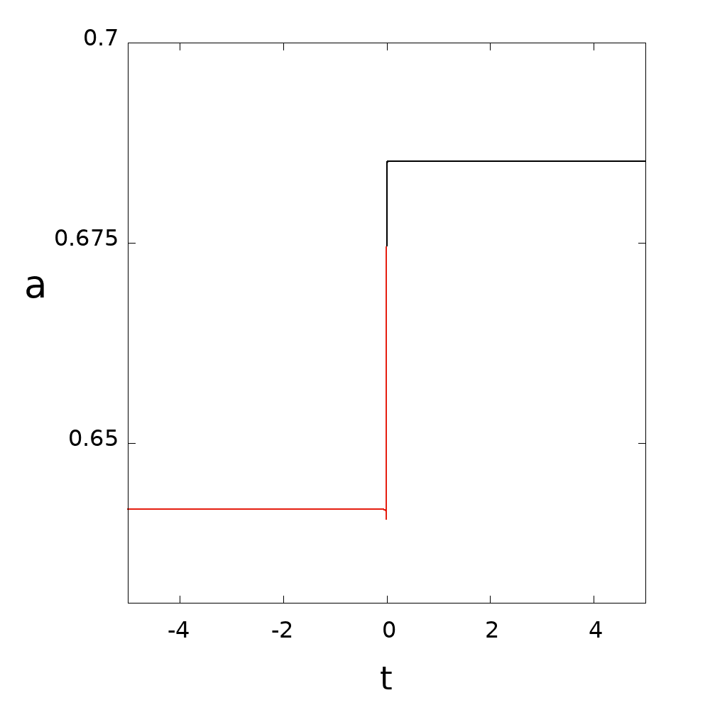
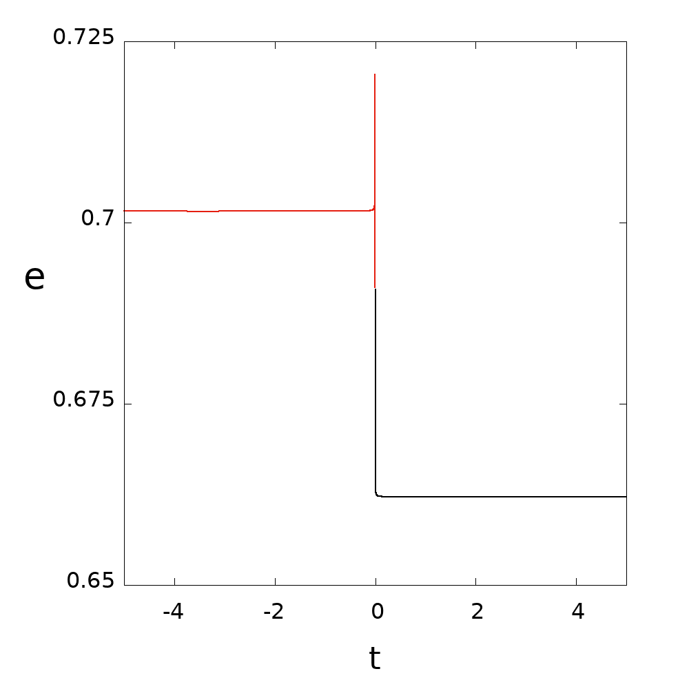
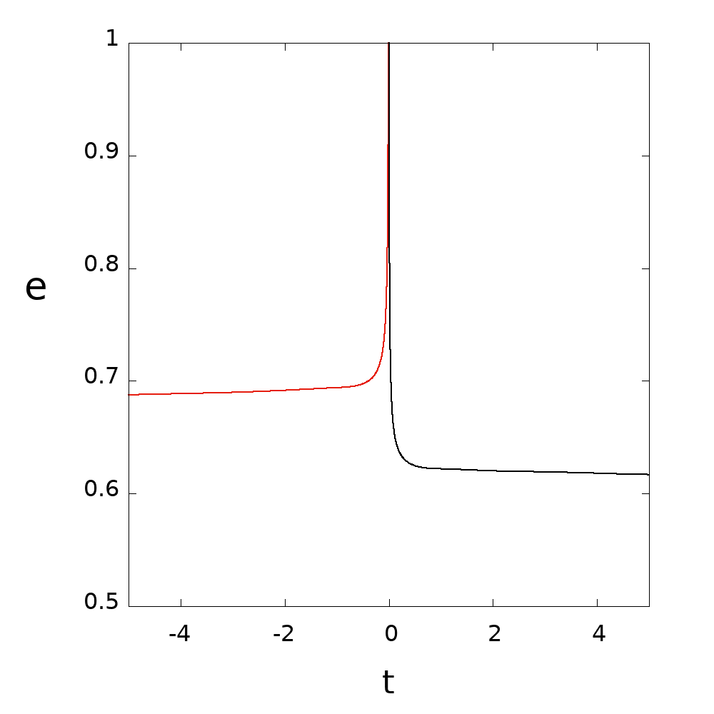
Figure 2: Representation of the time evolution of the semi-major axis $a$ and eccentricity $e$ for the orbits represented in Fig. 1: the top panels refer to the case $\mu=3\ 10^{-6}$, the bottom panels to the case $\mu=10^{-6}$.

The most important parameters of the problem are the mass parameter $\mu$ and the value $E$ of the Hamiltonian characterizing the close encounter. We consider two numerical values for the mass parameter $\mu=10^{-3}$ and $\mu=3.\ 10^{-6}$ which are representative, up to a small correction, of the three-body problems which are defined by considering the couples Sun–Jupiter and Sun–Earth as primary bodies respectively. The method considered in this paper applies to the fast close encounters, whose parameter $E$ satisfies inequality (2). Since the parameter $\lambda=\alpha/2>0$ is a divisor of the Bnf, the values of $\alpha$ close to zero (and in general $\alpha/2\in(0,1)$) imply larger coefficients of the monomials of the Bnf as well as larger errors in the representation of the solutions transiting at a given distance from $P_{2}$. Therefore, we consider the value of $E=-1.35$ which is close to the limit value $\alpha=0$ (precisely the small divisor in this case is $\alpha/2\sim 0.27$); the results are expected to improve for larger values of $E$.

For each value of $\mu$, we choose an initial condition $u(0),U(0)$ well inside the Hill’s sphere of the secondary body and we numerically compute its orbit for positive and negative times; this is equivalent to consider orbits having a close encounter with $P_{2}$. The orbits corresponding to the selected initial conditions are computed by numerically integrating the Hamilton’s equations of the Levi-Civita Hamiltonian using an explicit Runge-Kutta algorithm of order 6, with a very small integration time step of $\tau=10^{-5}$, and extended floating point numerical precision (the absolute value of the regularized Hamiltonian remains smaller than $3.5\ 10^{-16}$).

The numerically computed solutions will be used to check the conservation of the integrals of motions of the first and second Birkhoff Normal Forms, and compared with the solutions provided in parametric form by the Eq. (55). Two orbits, numerically computed for positive (black curve) and negative times (red curve), are represented in Fig. 1 for the case $\mu=3\ 10^{-6}$ and $\mu=10^{-3}$ respectively. The time variations of the semi-major axis $a$ and eccentricity $e$ are reported in Fig. 2: we appreciate that there is a sharp variation of $a$, $e$ in both cases, associated to the close encounter; in the case of the smaller mass value $\mu=3\ 10^{-6}$ the variation is almost stepwise.

These orbits are then analyzed using the Birkhoff normalizations described in Sections 2 and 4. The canonical transformations and the normal form Hamiltonian ${\hat{H}}^{N}_{E}$ are computed by implementing with a computer algebra system the algorithm described in Appendix 1 (Section 6). The implementation of the Birkhoff transformations requires:

• the computation of Taylor expansions of functions up to a given polynomial order $N$;

• the computation of the generating functions $\chi_{J}$ from the Taylor expansion of the Hamiltonian represented with the hyperbolic variables;

• the computation of the Lie series defined by $\chi_{J}$ up to the degree $N$.

The operations required by these three steps are performed by several available computer algebra systems. The implementation can be symbolic, i.e. the coefficients of all the monomials are given as functions of the parameters $\mu,\alpha$ (and no floating point approximations are introduced), or numeric, i.e. for a given value of $\mu,\alpha$ the coefficients of all the monomials are given as floating point numbers. The second choice allows to reach larger orders $N$. A symbolic implementation has been executed up to $N=20$; a numerical implementation (where $\mu,E$ are treated as floating point numbers) has been executed up to $N=30$, and this is the procedure whose results are reported below. In the numerical implementation the generating functions and the Birkhoff normal forms Hamiltonians are computed as polynomials with floating point coefficients. The canonical transformations, which are the flow at time $\tau=1$ (or $\tau=-1$ for the inverse) of the generating functions, can be also represented by polynomials. The direct numerical evaluation of these polynomials along the flow is computationally expensive; a less expensive evaluation (which is used in the computations described below) is obtained by numerically computing the Hamiltonian flow of the generating functions using an explicit Runge-Kutta algorithm of order 6 with $100$ steps.

For each orbit:

• we compute the function

  $$J^{N}=q_{1}p_{1}+q_{2}p_{2}$$

  along the numerically computed orbit for different orders of the first Birkhoff normalization ranging from $N=2$ (no normalization) up to $N=30$. We also check the conservation of the actions $Q_{1}P_{1}$ and $Q_{2}P_{2}$ for different normalization orders of the second Birkhoff normalization (which are implemented from the first Bnf of order $N=30$). Since the real and imaginary parts of $Q_{1}P_{1}$, $Q_{2}P_{2}$ are proportional to $q_{1}p_{1}+q_{2}p_{2}$ (which is already conserved up to order $N=30$ from the first Bnf) or $q_{1}p_{2}-q_{2}p_{1}$, we just need to check the conservation of

  $$W^{N,\tilde{N}}=\Im(Q_{1}P_{1})$$

  along the numerically computed orbits ($N$ refers to the order of the first Bnf, $\tilde{N}$ to the order of the second Bnf). The relative variations of $J^{N},W^{N,\tilde{N}}$ are represented versus the distance $r=|u|^{2}$ from the secondary body, providing us an estimate of the error which we have at some distance from $P_{2}$ using different normalization orders. In fact, the approximation of the solutions of the three-body problem with the solutions of the Hamilton’s equations of Hamiltonian (47) during the transit inside a sphere centered at $P_{2}$ of radius $\rho$ is justified if the variations of the function $J^{N},W^{N,\tilde{N}}$ remain extremely small during the transit, possibly smaller than the numerical precision.

• for the same initial conditions of the numerical integrations we also compute the solution provided by the parametric representation of Eq. (55) (mapped back to the original Levi-Civita variables $u,U$). The difference between the parametric and the numerical solution is represented versus the distance $|u|^{2}$ for different normalization orders.

During the fast close encounters, the orbits have a sharp change of the semi-major axis and eccentricity (see Fig. 2). In the left panels of Fig.s 3 and 4 we represent the relative variations:

$${\rm DJ}={|J^{N}(q(t),p(t))-J^{N}(q(0),q(0))|\over|J^{N}(q(0),q(0))|}$$ (56)

for different orders of the first Birkhoff normalization ranging from $N=2$ (no normalization) up to $N=30$, computed during the close encounter occurring from initial time until $P$ reaches a distance $r=0.1$ from $P_{2}$, for the orbit of the case $\mu=3\ 10^{-6}$ (Fig. 3) and $\mu=10^{-3}$ (Fig. 4). The relative variations are indeed extremely small for $N=30$ ($\sim 10^{-15}$ ) up to $r\sim 0.02$ for both orbits, with a possible improvement which still could be obtained by considering larger values of $N$. In the same panels we also report the relative variation of $W^{N,\tilde{N}}$, computed after the $N=30$ normalizations of the first Bnf:

$${\rm DW}={|W^{N,\tilde{N}}(q(t),p(t))-W^{N,\tilde{N}}(q(0),q(0))|\over|W^{N,\tilde{N}}(q(0),q(0))|},$$ (57)

which is very small up to $r\sim 0.02$ already for $\tilde{N}=10$ (Fig. 3) and $\tilde{N}=16$ (Fig. 4) respectively.

In the left panels of (Fig. 3) and (Fig. 4) we represent the distance:

$${\rm DIST}=\|(x^{N}-x^{P},y^{N}-y^{P})\|$$ (58)

in Cartesian variables $(x,y)$ between the solutions $(x^{N},y^{N})$ computed by numerically integrating the Hamilton’s equations of the Levi Civita Hamiltonian and the solutions $(x^{P},y^{P})$ provided by the parametric representation (55): the distances are smaller than $10^{-16}$ up to $r=0.02$.

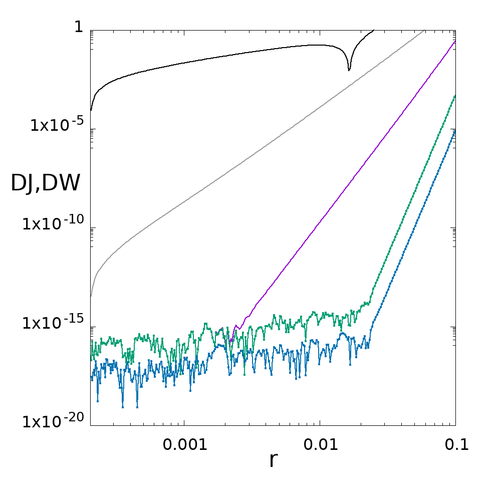
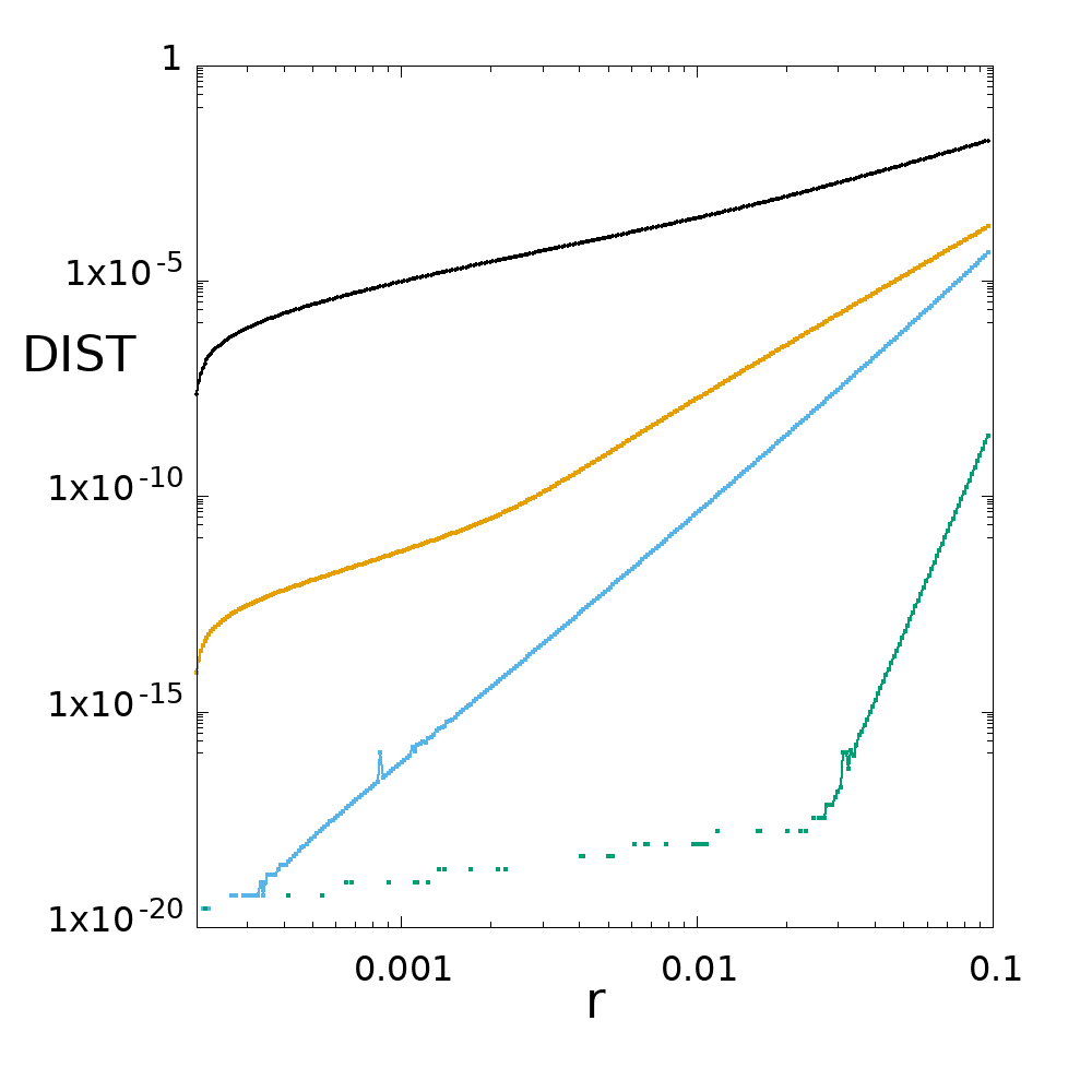
Figure 3: Left panel: Relative variation ${\rm DJ}$ (defined in Eq. (56)) computed for the same orbit of Fig. 1, top panels (case $\mu=3\ 10^{-6}$) represented versus the distance $r:=|u|^{2}$ from $P_{2}$ for $N=2$ (black) and the improvements provided by the Birkhoff normalizations with $N=8$ (gray), $N=16$, (violet), $N=30$ (green). The blue line represents instead the relative variation ${\rm DW}$ (defined in Eq. (57)) computed for $N=30,\tilde{N}=12$. Right panel: variation of ${\rm DIST}$ (defined in Eq. (58)) represented versus the distance $r:=|u|^{2}$ for $N,\tilde{N}=2$ (black) and the improvements provided by the Birkhoff normalizations with $N,\tilde{N}=4$ (gold), $N,\tilde{N}=10$ (light blue), $N=30,\tilde{N}=14$ (green).

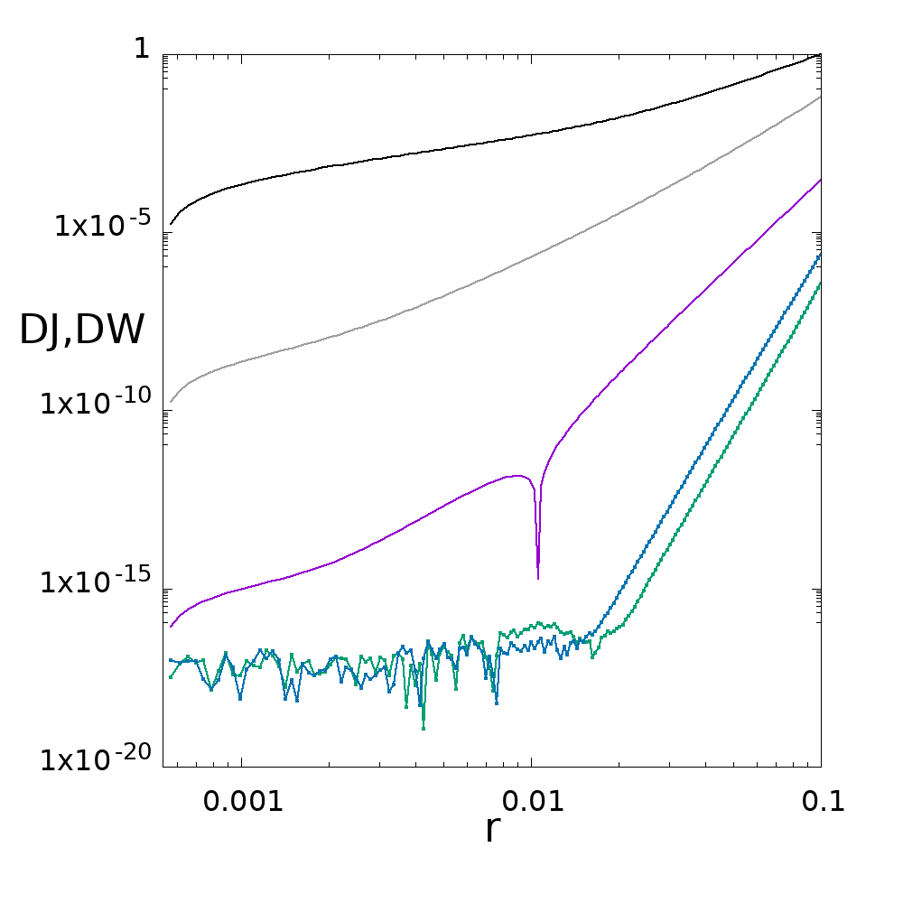
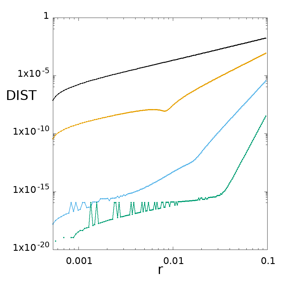
Figure 4: Left panel: Relative variation $DJ$ (defined in Eq. (56)) computed for the same orbit of Fig. 1, bottom panels (case $\mu=10^{-3}$) represented versus the distance $r:=|u|^{2}$ for $N=2$ (black) and the improvements provided by the Birkhoff normalizations with $N=8$ (gray), $N=16$, (violet), $N=30$ (green). The blue line represents instead the relative variation ${\rm DW}$ (defined in Eq. (57)) computed for $N=30,\tilde{N}=16$. Right panel: variation of ${\rm DIST}$ (defined in Eq. (58)) represented versus the distance $r:=|u|^{2}$ for $N=\tilde{N}=2$ (black), and the improvements provided by the Birkhoff normalizations with $N,\tilde{N}=4$ (gold), $N,\tilde{N}=14$ (light blue), $N=30,\tilde{N}=14$ (green).

6 Appendix 1: definition of the Birkhoff normal forms for 2-degrees of freedom Hamiltonians

Consider the 2-degrees of freedom Hamiltonian system of the form:

$$H(q,p)=h_{2}(q,p)+h_{4}(q,p)+h_{6}(q,p)....$$ (59)

where:

$$h_{2}(q,p)=\lambda_{1}q_{1}p_{1}+\lambda_{2}q_{2}p_{2},$$

and the functions $h_{2j}(q,p)$ are polynomials of degree $2j$.

For any even number $N\geq 4$, we apply iteratively a finite sequence of canonical transformations, called Birkhoff normalizations, whose composition is a close to the identity canonical transformation defined in a neighbourhood of $(q,p)=(0,0,0,0)$ (which is a fixed point of the transformation), conjugating $H$ to

$$H^{N}(q,p)=h_{2}(q,p)+{\hat{h}}_{4}(q,p)+\ldots+{\hat{h}}_{N}(q,p)+{\cal R}_{N+2}(q,p)$$ (60)

where ${\cal R}_{N+2}$ is a series in $q,p$ starting with terms of degree at least $N+2$ and the ${\hat{h}}_{j}$ are polynomials of order $j$ in $q,p$ (only the polynomials with $j$ even number appear in the expansion) containing monomials:

$$c^{j,N}_{m,n}q_{1}^{m_{1}}q_{2}^{m_{2}}p_{1}^{n_{1}}p_{2}^{n_{2}}$$ (61)

with $m=(m_{1},m_{2}),n=(n_{1},n_{2})$ satisfying:

$$\lambda_{1}(n_{1}-m_{1})+\lambda_{2}(n_{2}-m_{2})=0.$$ (62)

The Hamiltonian which is obtained by neglecting the remainder ${\cal R}_{N+2}(q,p)$ in ${H}^{N}(q,p)$:

$${\hat{H}}^{N}(q,p)=h_{2}(q,p)+{\hat{h}}_{4}(q,p)+\ldots+{\hat{h}}_{N}(q,p),$$

will be called Birkhoff normal form of $H$ of order $N$. The Birkhoff transformations and the transformed Hamiltonians can be computed explicitly with a computer algebra system, by representing them with the Lie series method (for a modern presentation of the Lie series method we refer to [12]), following the procedure described below.

The Birkhoff normalization of Hamiltonian (59) is obtained, for any $N\geq 4$, with a canonical transformation ${\cal C}_{N}$ defined as the composition of a sequence of canonical Birkhoff transformations:

$$(q,p):=(q^{(2)},p^{(2)})\mapsto(q^{(4)},p^{(4)})\mapsto\ldots\mapsto(q^{(N)},p^{(N)})$$ (63)

where each elementary transformation:

$$(q^{(J-2)},p^{(J-2)})=\Phi^{1}_{\chi_{{}_{J}}}(q^{(J)},p^{(J)}))$$ (64)

is the Hamiltonian flow $\Phi^{1}_{\chi_{{}_{J}}}$ at time $1$ of an Hamiltonian $\chi_{{}_{J}}$, which is polynomial of degree $J$. The elementary transformations (64) can be computed explicitly as the Lie series:

$$\zeta=\Big{[}e^{\,L_{\chi_{{}_{J}}}}\zeta\Big{]}(q^{(J)},p^{(J)}):=\zeta^{\prime}+\{\zeta,\chi_{{}_{J}}\}(q^{(J)},p^{(J)})+{1\over 2}\{\{\zeta,\chi_{J}\},\chi_{{}_{J}}\}(q^{(J)},p^{(J)})+\ldots~{},$$ (65)

where $L_{\chi_{{}_{J}}}:=\{\cdot,\chi_{{}_{J}}\}$, and $\zeta,\zeta^{\prime}$ denote any couple of variables ${{q}}^{(J-2)},{{q}}^{(J)}$ or ${{p}}^{(J-2)},{{p}}^{(J)}$. The Hamiltonian $H^{(2)}:=H$ is conjugate to the sequence of Hamiltonians $H^{(4)},\ldots,H^{(J)}$ which can be computed as Lie series as well:

$${H}^{(J)}=e^{L_{\chi_{{}_{J}}}}\,{H}^{(J-2)},$$ (66)

and the iteration ends for $J=N$. The aim is to define the generating functions $\chi_{{}_{J}}$ such that, at any step $J$, the intermediate normalized Hamiltonians:

$${H}^{(J)}:=h_{2}+\sum_{j=2}^{J\over 2}{H}^{(J)}_{2j}+\sum_{j\geq(J+2)/2}{\tilde{H}}^{(J)}_{2j}$$ (67)

have the property that $H^{(J)}_{2j}$ and ${\tilde{H}}^{(J)}_{2j}$ are polynomials of degree $2j$, and moreover $H^{(J)}_{2j}$ contain only monomials satisfying:

$$\lambda_{1}(n_{1}-m_{1})+\lambda_{2}(n_{2}-m_{2})=0.$$ (68)

We suppose that the Hamiltonian has been normalized up to given $J\geq 4$, and we define the subsequent normalization with a generating function $\chi_{{}_{J+2}}$ which is polynomial of degree $J+2$. Therefore, from the representation (67), we have:

$${H}^{(J+2)}=h_{2}+\sum_{j=2}^{J\over 2}{H}^{(J)}_{2j}+(\{h_{2},\chi_{{}_{J+2}}\}+{\tilde{H}}^{(J)}_{J+2})+{\cal O}(J+4),$$

whose term of degree $J+2$ is $\{h_{2},\chi_{{}_{J+2}}\}+{\tilde{H}}^{(J)}_{J+2}$. By denoting with $a^{(J)}_{m_{1},m_{2},n_{1},n_{2}}q_{1}^{m_{1}}q_{2}^{m_{2}}p_{1}^{n_{1}}p_{2}^{n_{2}}$ the monomials of ${\tilde{H}}^{(J)}_{J+2}$, and defining the generating function ${\chi_{{}_{J+2}}}$ by:

$$\chi_{{}_{J+2}}=\sum_{\begin{subarray}{c}(m_{1},m_{2},n_{1},n_{2})\in{\cal L}_{J+2}\end{subarray}}\frac{a^{(J)}_{m_{1},m_{2},n_{1},n_{2}}}{[\lambda_{1}(m_{1}-n_{1})+\lambda_{2}(m_{2}-n_{2})]}\,{q}_{1}^{m_{1}}{q}_{2}^{m_{2}}{p}_{1}^{n_{1}}{p}_{2}^{n_{2}}$$ (69)

where:

$${\cal L}_{{}_{J}}=\left\{(m_{1},m_{2},n_{1},n_{2})\in{\mathbb{N}}^{4}:\sum_{j=1}^{2}(n_{j}+m_{j})=J,\ {\rm and}\ \ \lambda_{1}(m_{1}-n_{1})+\lambda_{2}(m_{2}-n_{2})\neq 0\right\}~{},$$

we have

$$\{h_{2},\chi_{{}_{J+2}}\}+{\tilde{H}}^{(J)}_{J+2}=\Pi{\tilde{H}}^{(J)}_{J+2}:=\sum_{m,n:|m|+|n|=J+2,\lambda_{1}(n_{1}-m_{1})+\lambda_{2}(n_{2}-m_{2})=0}a^{(J)}_{m,n}q^{m}p^{n}.$$ (70)

Therefore, ${H}^{(J+2)}$ is normalized up to degree $J+2$. Since the generating function $\chi_{{}_{J}}$ is polynomial of order larger than $4$, its flow at time 1 is close to the identity and has the origin $(q,p)=(0,0,0,0)$ as a fixed point.

7 Appendix 2: the Birkhoff normalization for $N=6$

The saddle-saddle Birkhoff normalization of order $N=6$ is obtained using the generating functions:

$$\chi_{4}=\frac{{p_{1}}^{2}{p_{2}}{q_{1}}}{8\alpha^{2}}-\frac{{p_{1}}^{3}{q_{2}}}{8\alpha^{2}}-\frac{{p_{1}}{p_{2}}^{2}{q_{2}}}{8\alpha^{2}}+\frac{{p_{1}}{q_{1}}^{2}{q_{2}}}{8\alpha^{2}}+\frac{{p_{1}}{q_{2}}^{3}}{8\alpha^{2}}+\frac{{p_{2}}^{3}{q_{1}}}{8\alpha^{2}}-\frac{{p_{2}}{q_{1}}^{3}}{8\alpha^{2}}-\frac{{p_{2}}{q_{1}}{q_{2}}^{2}}{8\alpha^{2}}$$

$$\chi_{6}=\frac{{p_{1}}^{2}{p_{2}}^{2}{q_{1}}^{2}(9{\mu}-11)}{32\alpha^{4}}-\frac{3{p_{1}}^{3}{p_{2}}^{2}{q_{1}}({\mu}-1)}{32\alpha^{4}}+\frac{{p_{1}}^{2}{p_{2}}^{2}{q_{2}}^{2}(9{\mu}-11)}{32\alpha^{4}}-\frac{3{p_{1}}^{2}{p_{2}}^{3}{q_{2}}({\mu}-1)}{32\alpha^{4}}+\frac{{p_{1}}^{4}{p_{2}}^{2}({\mu}-1)}{64\alpha^{4}}+\frac{{p_{1}}^{2}{p_{2}}^{4}({\mu}-1)}{64\alpha^{4}}+\frac{{p_{1}}^{3}{p_{2}}{q_{1}}{q_{2}}(3{\mu}-2)}{8\alpha^{4}}-\frac{3{p_{1}}^{4}{p_{2}}{q_{2}}({\mu}-1)}{64\alpha^{4}}+\frac{{p_{1}}^{2}{q_{1}}^{2}{q_{2}}^{2}(11-9{\mu})}{32\alpha^{4}}-\frac{15{p_{1}}^{4}{q_{1}}^{2}({\mu}-1)}{64\alpha^{4}}+\frac{15{p_{1}}^{2}{q_{1}}^{4}({\mu}-1)}{64\alpha^{4}}+\frac{3{p_{1}}^{5}{q_{1}}({\mu}-1)}{64\alpha^{4}}+\frac{{p_{1}}^{4}{q_{2}}^{2}(3{\mu}-7)}{64\alpha^{4}}+\frac{{p_{1}}^{2}{q_{2}}^{4}(7-3{\mu})}{64\alpha^{4}}-\frac{{p_{1}}^{6}({\mu}-1)}{192\alpha^{4}}+\frac{{p_{1}}{p_{2}}^{3}{q_{1}}{q_{2}}(3{\mu}-2)}{8\alpha^{4}}-\frac{3{p_{1}}{p_{2}}^{4}{q_{1}}({\mu}-1)}{64\alpha^{4}}+\frac{{p_{1}}{p_{2}}{q_{1}}^{3}{q_{2}}(2-3{\mu})}{8\alpha^{4}}+\frac{{p_{1}}{p_{2}}{q_{1}}{q_{2}}^{3}(2-3{\mu})}{8\alpha^{4}}+\frac{3{p_{1}}{q_{1}}^{3}{q_{2}}^{2}({\mu}-1)}{32\alpha^{4}}-\frac{3{p_{1}}{q_{1}}^{5}({\mu}-1)}{64\alpha^{4}}+\frac{3{p_{1}}{q_{1}}{q_{2}}^{4}({\mu}-1)}{64\alpha^{4}}+\frac{{p_{2}}^{2}{q_{1}}^{2}{q_{2}}^{2}(11-9{\mu})}{32\alpha^{4}}+\frac{{p_{2}}^{2}{q_{1}}^{4}(7-3{\mu})}{64\alpha^{4}}+\frac{{p_{2}}^{4}{q_{1}}^{2}(3{\mu}-7)}{64\alpha^{4}}+\frac{15{p_{2}}^{2}{q_{2}}^{4}({\mu}-1)}{64\alpha^{4}}-\frac{15{p_{2}}^{4}{q_{2}}^{2}({\mu}-1)}{64\alpha^{4}}+\frac{3{p_{2}}^{5}{q_{2}}({\mu}-1)}{64\alpha^{4}}-\frac{{p_{2}}^{6}({\mu}-1)}{192\alpha^{4}}+\frac{3{p_{2}}{q_{1}}^{2}{q_{2}}^{3}({\mu}-1)}{32\alpha^{4}}+\frac{3{p_{2}}{q_{1}}^{4}{q_{2}}({\mu}-1)}{64\alpha^{4}}-\frac{3{p_{2}}{q_{2}}^{5}({\mu}-1)}{64\alpha^{4}}-\frac{{q_{1}}^{2}{q_{2}}^{4}({\mu}-1)}{64\alpha^{4}}-\frac{{q_{1}}^{4}{q_{2}}^{2}({\mu}-1)}{64\alpha^{4}}+\frac{{q_{1}}^{6}({\mu}-1)}{192\alpha^{4}}+\frac{{q_{2}}^{6}({\mu}-1)}{192\alpha^{4}}$$

The focus-focus Birkhoff normalization of order $N=6$ is obtained using the generating functions:

$$\chi_{4}=\frac{15i{P_{2}}^{2}{Q_{1}}^{2}(\mu-1)}{32\alpha^{2}}-\frac{15i{P_{1}}^{2}{Q_{2}}^{2}(\mu-1)}{32\alpha^{2}}$$

$$\chi_{6}=\frac{15i{P_{1}}^{2}{P_{2}}{Q_{1}}^{3}(\mu-1)}{128\alpha^{3}}-\frac{75i{P_{1}}^{2}{P_{2}}{Q_{1}}{Q_{2}}^{2}(\mu-1)}{128\alpha^{3}}-\frac{45{P_{1}}^{2}{P_{2}}{Q_{2}}^{3}\left(\mu^{2}-6\mu+5\right)}{256\alpha^{4}}-\frac{15i{P_{1}}^{3}{Q_{1}}^{2}{Q_{2}}(\mu-1)}{128\alpha^{3}}+\frac{45{P_{1}}^{3}{Q_{1}}{Q_{2}}^{2}\left(\mu^{2}-6\mu+5\right)}{256\alpha^{4}}-\frac{175i{P_{1}}^{3}{Q_{2}}^{3}(\mu-1)}{384\alpha^{3}}+\frac{75i{P_{1}}{P_{2}}^{2}{Q_{1}}^{2}{Q_{2}}(\mu-1)}{128\alpha^{3}}-\frac{45{P_{1}}{P_{2}}^{2}{Q_{1}}^{3}\left(\mu^{2}-6\mu+5\right)}{256\alpha^{4}}-\frac{15i{P_{1}}{P_{2}}^{2}{Q_{2}}^{3}(\mu-1)}{128\alpha^{3}}+\frac{45{P_{2}}^{3}{Q_{1}}^{2}{Q_{2}}\left(\mu^{2}-6\mu+5\right)}{256\alpha^{4}}+\frac{175i{P_{2}}^{3}{Q_{1}}^{3}(\mu-1)}{384\alpha^{3}}+\frac{15i{P_{2}}^{3}{Q_{1}}{Q_{2}}^{2}(\mu-1)}{128\alpha^{3}}$$

8 Conclusions and perspectives

The method presented in this paper allows to compute the close encounters with the secondary body of the planar circular restricted three–body problem using integrable dynamics approximating the regularized Hamiltonian at any order $N$ of its Birkhoff approximations. The numerical implementations of the method show that it indeed can be applied to problems whose parameters are compatible with important Solar System three-body problems, with errors on the predicted orbits which can be reduced below the round-off approximation. Therefore, it provides an Hamiltonian integrator of the close encounters as a single step.

We have therefore the opportunity to compare the output of numerical integrations with these Hamiltonian dynamics to confirm their correctness when they agree below a precision threshold. In fact, there is no way to state the correctness of the numerical integration of a close encounter, a part from the necessary conservation of the Hamiltonian (which implies the approximate conservation of the Tisserand parameter before and after the close encounter).

In future researches, applications of the method for a full range of parameters $\mu,E$ which are relevant for Solar system applications will be investigated, as well as possible extensions to models which are more representative of the dynamics of a realistic model of the Solar System.

Acknowledgments. The author thanks prof.s E. Detomi and A. Lucchini for presenting to me the sufficient condition for the factorization of polynomials of four variables. He also acknowledges the project MIUR-PRIN 20178CJA2B “New frontiers of Celestial Mechanics: theory and applications”.

References

- [1] Arenstorf R.F., Periodic solutions of the restricted three-body problem representing analytic continuations of Keplerian elliptic motions, Amer. J. Math., 85, pp. 27-35, 1963.
- [2] Bolotin, S.V., MacKay, R.S.: Periodic and chaotic trajectories of the second species for the n-centre problem. Celest. Mech. Dyn. Astron. 77, 49–75, 2000.
- [3] Bolotin S., Shadowing chains of collision orbits. Discr. Conts. Dyn. Syst. 14, 235–260, 2006.
- [4] Capiński M.J., Kepley S., Mireles James, J.D., Computer assisted proofs for transverse collision and near collision orbits in the restricted three body problem, Journal of Differential Equations, Vol, 366, 132-191, 2023.
- [5] Cardin F. and Guzzo M. “Integrability of close encounters in the spatial restricted three-body problem”. Accepted for publication by Comm. Cont. Math. 2021.
- [6] Ceccaroni, M., Celletti, A. and Pucacco G., Halo orbits around the collinear points of the restricted three-body problem. Physica D, Volume 317, 1, p. 28-42, 2016.
- [7] Chenciner A., Llibre J., A note on the existence of invariant punctured tori in the planar circular restricted three-body problem, Ergod. Theory Dyn. Syst. (Charles Conley Memorial Issue) 8, 63–72, 1988.
- [8] Clairaut A.-C., Thèorie du mouvement des comètes, Paris, 1760.
- [9] Féjoz J., Quasiperiodic motions in the planar three-body problem, J. Differ. Equ. 183, 2, 303–341, 2002.
- [10] Font J., Nunes A., Simó C., Consecutive quasi-collisions in the planar circular RTBP, Nonlinearity, 15, 115, 2002.
- [11] Font J., Nunes A., Simó C., A numerical study of the orbits of second species of the planar circular RTBP, Celest. Mech. Dyn. Astron. 103, 2, 143–162, 2009.
- [12] Giorgilli A., Notes on Hamiltonian Dynamical Systems. Cambridge University Press, 2022.
- [13] Gómez G., Jorba À., Masdemont J., Simó C., Dynamics and Mission Design Near Libration Point Orbits, Vol. 3: Advanced Methods for Collinear Points, World Scientific, Singapore, 2000.
- [14] Jacobson N., Basic Algebra 1, W. H. Freeman and Co., San Francisco, CA, 1974, second edition 1985.
- [15] Jorba A., Masdemont J., Dynamics in the center manifold of the restricted three-body problem, Physica D 132, 189-213, 1999.
- [16] Guardia M., Kaloshin V., Zhang J., Asymptotic Density of Collision Orbits in the Restricted Circular Planar 3 Body Problem, Archive for Rational Mechanics and Analysis, vol. 233, Issue 2, pp 799-836, 2019.
- [17] Halley E., A Synopsis of the Astronomy of Comets, 1705.
- [18] Hénon, M.R.: Generating Families in the Restricted Three Body Problem, Lect. Notes in Phys. Monographs, 52, Springer, Berlin, 1997.
- [19] Henrard J. “On Poincaré’s second species solutions”. In Cel. Mech., vol 21, 83-97, 1980.
- [20] Levi-Civita T. “Sur la régularisation qualitative du probléme restreint des trois corps”. In: Acta Math. 30 (1906), pp. 305-327.
- [21] Laplace P.S., Traité de Mécanique Céleste, T. IV, Livre IX, Chapitre II, Paris, 1880.
- [22] Le Verrier U.J., Théorie de la comete périodique de 1770, Annales de l’Observatoire imperial de Paris, Memoires, t. 3. Paris: Mallet-Bachelier, p. 203-270, 1-12, 1857.
- [23] Marco J.-P., Niederman L., Sur la construction des solutions de seconde espèce dans le problème plan restreint des trois corps, Ann. Inst. H. Poincaré Phys. Théor. 62, 211–249, 1995.
- [24] Masdemont J.J., High Order Expansions of Invariant Manifolds of Libration Point Orbits with Applications to Mission Design, Dynamical Systems: An International Journal, vol. 20, no. 1, pp. 59-113, 2005.
- [25] Perko L.M., Periodic Orbits in the Restricted Three-Body Problem: Existence and Asymptotic Approximation, Siam J. Appl. Math. 41, 200-237, 1974.
- [26] Paez R.I., Guzzo M., A study of temporary captures and collisions in the Circular Restricted Three-Body Problem with normalizations of the Levi-Civita Hamiltonian, Int. J. of Non-Lin. Mech., 120, 103417, 2020.
- [27] Paez R.I. and Guzzo M. Transits close to the Lagrangian solutions , in the elliptic restricted three-body problem, Nonlinearity, 34 (2021), 6417-6449.
- [28] Paez R.I., Guzzo M., On the semi-analytical construction of halo orbits and halo tubes in the elliptic restricted three-body problem, Physica D: Nonlinear Phenomena 439, 133402, 2022.
- [29] Peterson L.T., Rosales J.J., Scheeres D.J., The Vicinity of Earth-Moon L1 and L2 in the Hill Restricted 4-Body Problem, Physica D: Nonlinear Phenomena, vol. 45, 133889, 2023.
- [30] Pucacco G., Structure of the centre manifold of the collinear libration points in the restricted three-body problem, Cel. Mech. and Dyn. Astr., 131, article number 44 (2019).
- [31] Rosales J.J., Jorba À., Jorba-Cuscó M., Invariant manifolds near L1 and L2 in the quasi-bicicurlar problem, Celestial Mechanics and Dynamical Astronomy 135, 15, 2023.
- [32] Simó C., Dynamical systems methods for space missions on a vicinity of collinear libration points, in Simó, C., editor, Hamiltonian Systems with Three or More Degrees of Freedom (S’Agaró, 1995), volume 533 of NATO Adv. Sci. Inst. Ser. C Math. Phys. Sci., pp. 223-241, Dordrecht. Kluwer Acad. Publ., 1999.
- [33] Tisserand F.F., Sur la théorie de la capture de comètes périodiques, Bulletin Astronomique, vol. 6, p. 241-257, 1889.
- [34] Zhao L., Quasi-periodic almost-collision orbits in the spatial three-body problem, Commun. Pure Appl. Math. 68, 12, 2144–2176, 2015.