Data Imbalance, Uncertainty Quantification, and Generalization via Transfer Learning in Data-driven Parameterizations: Lessons from the Emulation of Gravity Wave Momentum Transport in WACCM
Abstract
Neural networks (NNs) are increasingly used for data-driven subgrid-scale parameterization in weather and climate models. While NNs are powerful tools for learning complex nonlinear relationships from data, there are several challenges in using them for parameterizations. Three of these challenges are 1) data imbalance related to learning rare (often large-amplitude) samples; 2) uncertainty quantification (UQ) of the predictions to provide an accuracy indicator; and 3) generalization to other climates, e.g., those with higher radiative forcing. Here, we examine performance of methods for addressing these challenges using NN-based emulators of the Whole Atmosphere Community Climate Model (WACCM) physics-based gravity wave (GW) parameterizations as the test case. WACCM has complex, state-of-the-art parameterizations for orography-, convection- and frontal-driven GWs. Convection- and orography-driven GWs have significant data imbalance due to the absence of convection or orography in many grid points. We address data imbalance using resampling and/or weighted loss functions, enabling the successful emulation of parameterizations for all three sources. We demonstrate that three UQ methods (Bayesian NNs, variational auto-encoders, and dropouts) provide ensemble spreads that correspond to accuracy during testing, offering criteria on when a NN gives inaccurate predictions. Finally, we show that accuracy of these NNs decreases for a warmer climate (CO2). However, the generalization accuracy is significantly improved by applying transfer learning, e.g., re-training only one layer using new data from the warmer climate. The findings of this study offer insights for developing reliable and generalizable data-driven parameterizations for various processes, including (but not limited) to GWs.
JAMES
Rice University, Houston, TX, 77005 NorthWest Research Associates, Boulder, CO, 80301, USA Pacific Northwest National Laboratory, Richland, WA, 99354, USA New York University, New York, NY 10012, USA Stanford University, Stanford, CA, 94305, USA
Y. Qiang Sun and Pedram Hassanzadehys91@rice.edu and pedramh@uchicago.edu
WACCM’s orographic, convective, and frontal gravity wave parameterizations are emulated using neural nets to inform future modeling efforts
Out-of-distribution generalization (extrapolation) of the neural nets under CO2 forcing is enabled via transfer learning with new data
Data imbalance is addressed via resampling and weighted loss; uncertainty quantification via Bayesian, dropout, and variational methods
Plain Language Summary
Scientists are increasingly using machine learning methods, especially neural networks (NNs), to improve weather and climate models. However, it can be challenging for a NN to learn rare, large-amplitude events, because they are infrequent in training data. Also, NNs need to express their confidence (certainty) about a prediction and work effectively across different climates, e.g., warmer climates due to increased CO2. Traditional NNs often struggle with these challenges. Here, we share insights gained from emulating the complex physics-based parameterization schemes for gravity waves in a state-of-the-art climate model. We propose specific strategies for addressing imbalanced data, uncertainty quantification (UQ), and making accurate predictions across various climates. For instance, to manage data balance, one such strategy involves amplifying the impact of infrequent events in the training data. We also demonstrate that several UQ methods could be useful in determining the accuracy of predictions. Furthermore, we show that NNs trained on simulations of the historical period do not perform as well in warmer climates. However, we improve the NNs’ performance by employing transfer learning using limited data from warmer climates. This study provides lessons for developing robust and generalizable approaches for using NNs to improve models in the future.
1 Introduction
Small-scale processes such as moist convection, gravity waves, and turbulence are key players in the variability of the climate system and its response to increased greenhouse gases. However, as these processes cannot be resolved, entirely or partially, by the coarse-resolution general circulation models (GCMs), they need to be represented as functions of the resolved dynamics via subgrid-scale (SGS) parameterization schemes (e.g., Kim \BOthers., \APACyear2003; Stensrud, \APACyear2007; Prein \BOthers., \APACyear2015). Many of these parameterization schemes are based on heuristic approximations and simplifications, introducing large parametric and epistemic uncertainties in GCMs (Schneider \BOthers., \APACyear2017; Hourdin \BOthers., \APACyear2017; Palmer, \APACyear2019).
Recently, there has been a growing interest in developing data-driven SGS parameterizations for different complex processes in the Earth system using machine learning (ML) techniques, particularly deep neural networks (NNs). Promising results have been demonstrated in a wide range of idealized applications, including prototype systems (Maulik \BOthers., \APACyear2019; Gagne \BOthers., \APACyear2020; Rasp, \APACyear2020; Chattopadhyay, Subel\BCBL \BBA Hassanzadeh, \APACyear2020; Frezat \BOthers., \APACyear2022; Guan \BOthers., \APACyear2022; Pahlavan \BOthers., \APACyear2023), ocean turbulent processes (Bolton \BBA Zanna, \APACyear2019; C. Zhang \BOthers., \APACyear2023), moist convection in the atmosphere (O’Gorman \BBA Dwyer, \APACyear2018; Brenowitz \BBA Bretherton, \APACyear2019; Yuval \BBA O’Gorman, \APACyear2020; Beucler \BOthers., \APACyear2021; Iglesias-Suarez \BOthers., \APACyear2023), radiation (Krasnopolsky \BOthers., \APACyear2005; Belochitski \BBA Krasnopolsky, \APACyear2021; Song \BBA Roh, \APACyear2021), and microphysics (Seifert \BBA Rasp, \APACyear2020; Gettelman \BOthers., \APACyear2021). The ultimate promise of data-driven parameterizations, learned from observation-derived data and/or high-fidelity high-resolution simulations, is that they might have smaller parametric/structural errors, thus reducing the biases of GCMs and producing more reliable climate change projections (e.g., Schneider \BOthers., \APACyear2017; Reichstein \BOthers., \APACyear2019; Schneider \BOthers., \APACyear2021).
However, there are major challenges in developing trustworthy, interpretable, stable, and generalizable data-driven parameterizations that can be used for such climate change projection efforts. Discussing and even listing all of these challenges is well beyond the scope of this paper. Well-known challenges such as interpretability and stability have been extensively discussed in a number of recent studies (e.g., McGovern \BOthers., \APACyear2019; Beck \BOthers., \APACyear2019; Brenowitz \BOthers., \APACyear2020; Balaji, \APACyear2021; Clare \BOthers., \APACyear2022; Mamalakis \BOthers., \APACyear2022; Guan \BOthers., \APACyear2022; Subel \BOthers., \APACyear2023; Pahlavan \BOthers., \APACyear2023). Here, we focus on three other key issues:
-
1.
Data imbalance, and related to that, learning rare/extreme events,
-
2.
Uncertainty quantification (UQ) of the NN-based SGS parameterization outputs,
-
3.
Out-of-distribution (OOD) generalization (e.g., extrapolation to climates with higher radiative forcings).
Below we briefly discuss the importance of 1-3 and the current state-of-the-art methods in addressing them in the climate and ML literature. Data imbalance is a well-known problem in the ML literature, especially in the context of classification tasks (e.g., Japkowicz \BBA Stephen, \APACyear2002; G. Wu \BBA Chang, \APACyear2003; Chawla \BOthers., \APACyear2004; Y. Sun \BOthers., \APACyear2009; Huang \BOthers., \APACyear2016; Ando \BBA Huang, \APACyear2017; Buda \BOthers., \APACyear2018; Johnson \BBA Khoshgoftaar, \APACyear2019). The problem becomes particularly significant when one aims to learn rare/extreme events (Maalouf \BBA Trafalis, \APACyear2011; Maalouf \BBA Siddiqi, \APACyear2014; Baldi \BOthers., \APACyear2014; Liu \BOthers., \APACyear2016; O’Gorman \BBA Dwyer, \APACyear2018; Qi \BBA Majda, \APACyear2020; Chattopadhyay, Nabizadeh\BCBL \BBA Hassanzadeh, \APACyear2020; Miloshevich \BOthers., \APACyear2023; Finkel \BOthers., \APACyear2023; Shamekh \BOthers., \APACyear2023). For example, suppose we aim to learn the binary classification of the 99 percentile of temperature anomalies using a NN. In this case, label 0 (no extreme) will constitute of the training (or testing) set while label 1 (extreme) will be just . With many common loss functions such as mean squared error (MSE) or root-mean squared-error (RMSE), training a NN will result in one that predicts 0 for any sample (extreme or no extreme) while having a seemingly high accuracy of (of course, other metrics such as precision/recall will show the shortcoming, see Chattopadhyay, Nabizadeh\BCBL \BBA Hassanzadeh (\APACyear2020)). The most common remedy to this problem for classification tasks is resampling. An example is down-sampling non-extreme cases by a factor of 100, which effectively balances the dataset.
In addition to classification tasks, Data imbalance also presents a significant challenge in regression tasks required for parameterization schemes in climate models. As highlighted by Chantry \BOthers. (\APACyear2021), such imbalances contributed to the unsuccessful emulation of their orographic gravity wave parameterization (GWP) scheme, largely because orography affects the gravity wave (GW) drag in only a fraction of the grid columns. This challenge also persists in emulating GWP for non-orographic GWs, especially when GWs are intricately linked to their sources. For instance, the presence of zero convective GW drag at numerous grid points due to the absence of convection creates a notably imbalanced dataset. This issue will be explored further in the results section. In regression tasks, data imbalance may also manifest in the form of difficulty in learning large-amplitude (extreme) outputs, which are rare and constitute only a small fraction of the training set. In the case of GWs, Observations have shown that gravity wave amplitudes are highly intermittent such that the largest 10% events alone can contribute more than 50% of the total momentum flux (Hertzog \BOthers., \APACyear2012), so the extreme events will contribute an outsized fraction of the total drag. Nonetheless, poorly learning these large-amplitude outputs, like drag forces, can result in instabilities (e.g., Guan \BOthers., \APACyear2022). Addressing data imbalance in climate applications has received relatively limited attention. In this study, we propose several remedies based on resampling techniques and weighted loss functions, demonstrating their advantages in enabling successful emulations of all GWP schemes and improving the learning of rare/extreme events.
Quantifying the uncertainties in outputs from NN-based parameterization schemes is essential when employing these schemes, particularly for high-stakes decision-making tasks such as climate change projections. Crucially, during testing when we are unable to directly determine a prediction’s accuracy, we need a UQ method that can provide a credible confidence level for each prediction, serving as a reliable indicator of its accuracy. During inference, the output of an NN can be inaccurate for various reasons, including poor approximation (e.g., due to poor NN architecture), poor within-distribution generalization (e.g., for inputs that are rare events), or poor optimization (collectively referred to as epistemic uncertainty), as well as because of OOD generalization errors due to input samples from a distribution different from that of the training set (Abdar \BOthers., \APACyear2021; Lu \BOthers., \APACyear2021; Krueger \BOthers., \APACyear2021; Miller \BOthers., \APACyear2021; Shen \BOthers., \APACyear2021; D. Wu \BOthers., \APACyear2021; Ye \BOthers., \APACyear2021; D. Zhang \BOthers., \APACyear2021; Subel \BOthers., \APACyear2023). Quantifying the level of uncertainty would then allow us to avoid using a data-driven parameterization scheme when it is inaccurate due to one of the aforementioned reasons (Maddox \BOthers., \APACyear2019; Zhu \BOthers., \APACyear2019; Li \BOthers., \APACyear2022; Psaros \BOthers., \APACyear2023). In the context of data-driven parameterization in climate modeling, the two most challenging sources of uncertainty are rare/extreme events and OOD generalization errors. The latter is a concern, particularly when the GCM is used for climate change studies (see below for more discussions).
Developing UQ methods for NNs is an active area of research in the ML community, and there is not a generally applicable rigorous method yet. For instance, techniques like Markov-Chain Monte Carlo can be prohibitively expensive, especially when dealing with high-dimensional systems (Oh \BOthers., \APACyear2005; Ballnus \BOthers., \APACyear2017; Chen \BBA Majda, \APACyear2019). For a comprehensive review in the context of scientific ML, refer to Psaros \BOthers. (\APACyear2023). The topic has also started to increasingly gain attention in the climate literature (Guillaumin \BBA Zanna, \APACyear2021; Gordon \BBA Barnes, \APACyear2022; Haynes \BOthers., \APACyear2023; Barnes \BOthers., \APACyear2023). In this study, we will assess the performance of three common UQ methods (Bayesian, dropout, and variational NNs) by analyzing the relationships between uncertainty and accuracy during inference testing. We will also consider scenarios involving OOD generalization errors resulting from global warming.
As already mentioned above, OOD generalization (extrapolation to a test data distribution different from that of the training set) is a major challenge for applications involving non-stationarity, like a changing climate. Studies have already shown that the lack of OOD generalization in data-driven parameterizations leads to inaccurate and unstable simulation (Rasp \BOthers., \APACyear2018; O’Gorman \BBA Dwyer, \APACyear2018; Chattopadhyay, Subel\BCBL \BBA Hassanzadeh, \APACyear2020; Guan \BOthers., \APACyear2022; Nagarajan \BOthers., \APACyear2020). A general and powerful method for improving the OOD generalization capability of NNs is transfer learning (TL), which involves re-training a few or all of the layers of a NN using a small amount of data from the new system (Yosinski \BOthers., \APACyear2014). This approach has already shown remarkable success in enabling data-driven parameterization schemes to extrapolate across the parameter space (e.g., to higher Reynolds number) in canonical test cases (Chattopadhyay, Subel\BCBL \BBA Hassanzadeh, \APACyear2020; Subel \BOthers., \APACyear2021; Guan \BOthers., \APACyear2023; Subel \BOthers., \APACyear2023; C. Zhang \BOthers., \APACyear2023). In particular, Subel \BOthers. (\APACyear2023) introduced SpArK (Spectral Analysis of Regression Kernels and Activations) showing that re-training even one layer can lead to successful OOD generalization, although this optimal layer, unlike the rule of thumb in the ML literature, may not be the deepest but the shallowest hidden layer. Here, we further leverage these studies and show how TL can enable OOD generalization of data-driven parameterization schemes in state-of-the-art GCMs.
The methods used in this study and the learned lessons apply to a broad range of processes and applications in climate modeling. However, the results are presented for a single test case, that is based on the emulation of complex physics-based GWP schemes in version 6 of the Whole Atmosphere Community Climate Model (WACCM), a state-of-the-art GCM (Gettelman \BOthers., \APACyear2019). Here, we use the emulations of current physics-based parameterization schemes as a stepping stone towards learning data-driven parameterizations from observations and high-fidelity simulations by testing ideas for addressing items 1-3 listed earlier. Furthermore, developing better representations of un- and under-resolved GWs in GCMs is an important problem on its own (Kim \BOthers., \APACyear2003; Alexander \BOthers., \APACyear2010; Achatz, \APACyear2022). A number of recent studies have taken the first steps in learning data-driven GWP from observations and high-resolution simulations (Matsuoka \BOthers., \APACyear2020; Amiramjadi \BOthers., \APACyear2022; Y\BPBIQ. Sun \BOthers., \APACyear2023; Dong \BOthers., \APACyear2023), though careful and time-consuming steps are needed in producing, analyzing, and using such data. Furthermore, two recent studies focused on emulators of simpler GWP schemes in a forecast model and idealized GCM have readily shown the usefulness of lessons learned from emulators (Chantry \BOthers., \APACyear2021; Espinosa \BOthers., \APACyear2022; Hardiman \BOthers., \APACyear2023). This further motivates the focus on using emulators for testing ideas for addressing data imbalance, UQ, and OOD generalization.
This paper is structured as follows. Section 2 introduces the WACCM simulations and the NN architectures used in this study. The findings, detailed in Section 3, emphasize the insights gained in addressing data imbalance and UQ, alongside OOD generalization of the emulators under warmer climate conditions. Consistent with Chantry \BOthers. (\APACyear2021), we find that using an NN to emulate the parameterization of orographic GWs is significantly more challenging than non-orographic GWs. This necessitated additional steps to achieve reasonable offline performance, as detailed in Section 4. To the best of our knowledge, this stands as the first NN-based emulation of orographic GWs to address the challenges in Chantry \BOthers. (\APACyear2021). Finally, we provide a concluding summary in Section 5.
2 Data and Methods
2.1 The Whole Atmosphere Community Climate Model (WACCM)
The NCAR’s WACCM version 6 introduced in Gettelman \BOthers. (\APACyear2019) is used in this study. WACCM has state-of-the-art GWP schemes for GWs from three different sources: orography (OGWs), convection (CGWs), and fronts (FGWs). These complex sources make the emulation of the GWP schemes in WACCM a challenging task. This is, therefore, a suitable test case to investigate ideas for learning rare events, UQ, and OOD generalization to benefit the future efforts for the much more complex task, that is learning data-driven GWP schemes from observations and/or high-resolution GW-resolving simulations (Amiramjadi \BOthers., \APACyear2022; Y\BPBIQ. Sun \BOthers., \APACyear2023).
The configuration of the WACCM used in this study is identical to the public version in Gettelman \BOthers. (\APACyear2019), with a horizontal resolution of and 70 vertical levels. The two non-orographic GWP schemes in WACCM both follow Richter \BOthers. (\APACyear2010), yet allow separate specifications of FGW and CGW sources. For OGWs, WACCM uses an updated planetary boundary layer form drag scheme from Beljaars \BOthers. (\APACyear2004), near-surface nonlinear drag processes following Scinocca \BBA McFarlane (\APACyear2000), and a ridge-finding algorithm to define orographic sources based on Bacmeister \BOthers. (\APACyear1994). A full documentation of WACCM OGWs can also be found in Kruse \BOthers. (\APACyear2022).
We conduct two sets of simulations: A 10-year pre-industrial “control” run, and a 10-year pseudo-global-warming “future” run with 4CO2 and uniform +4 K sea-surface temperature increases. In each run, we save, on the native grid, all the inputs and outputs for each of the three GWPs every 3 hours to capture the diurnal cycle. A complete list of these inputs/outputs, which are used in the training of the NN-based emulators, is presented in A.
We train separate NNs for emulating the three GWP schemes that have different sources. We use the first 6 years of the control run for training and the last 4 years for validation (years 7 and 8) and testing (years 9 and 10). With a grid resolution of 1∘, there are 55,296 columns for each time snapshot, resulting in approximately 960 million input/output columns during the 6-year training period. Given the strong temporal correlation between the 3-hourly samples, we perform sub-sampling on both the training and validation data to reduce the dataset size. To accomplish this, we begin by shuffling all the input/output column pairs in time at each latitude/longitude grid point. Then, we randomly select 2,000 input/output pairs at each location for training and 500 pairs for validation.
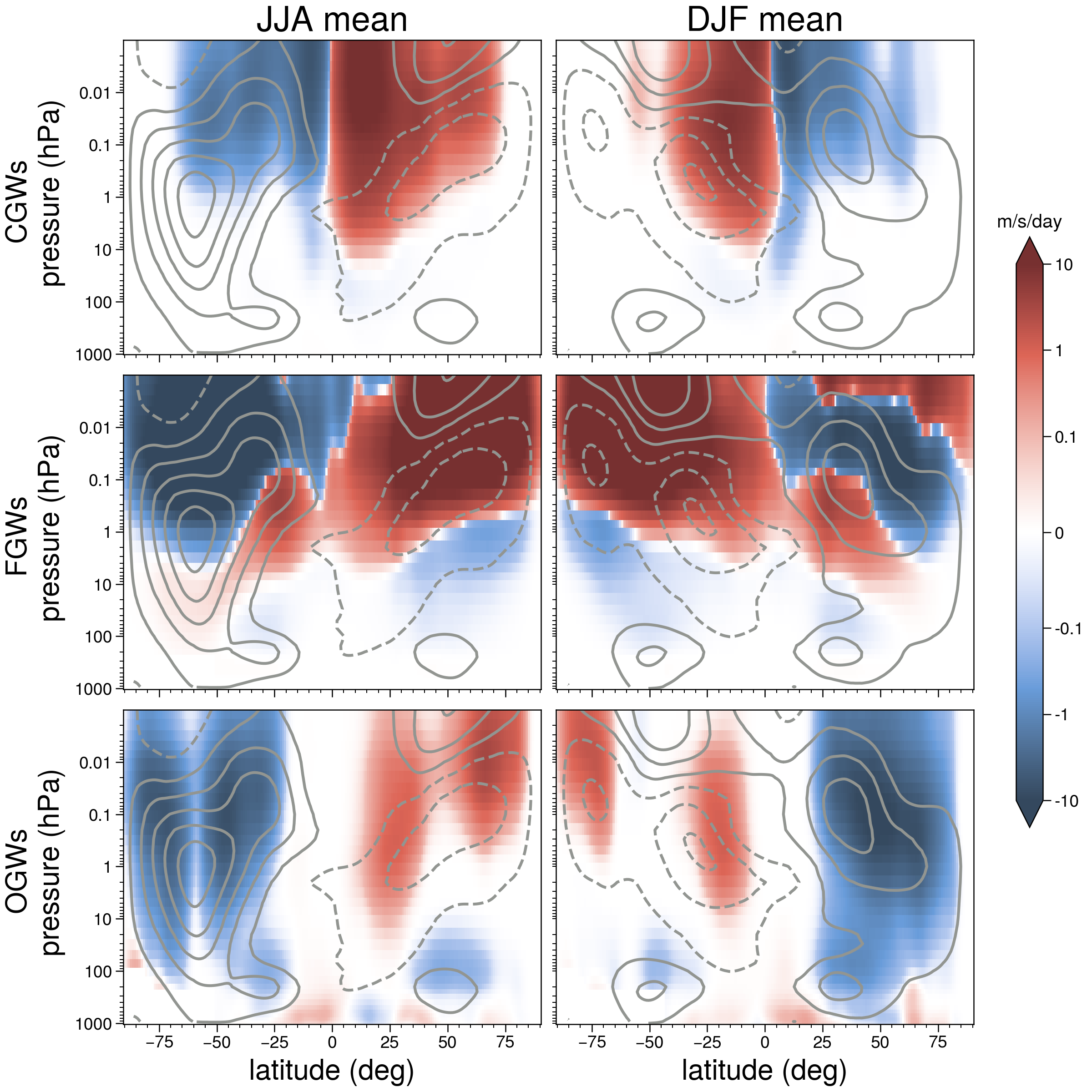
To give the readers a general idea of the parameterized GWs and large-scale circulation in WACCM, Figure 1 shows the zonal-mean climatology for zonal GW drag/forcing, hereinafter referred to as GWD, arises from the divergence of gravity wave momentum transport (fluxes), from all three sources, computed from the 6-year training period in the control run. The zonal-mean zonal wind climatology is also shown. Seasonal dependency for both the GWD and the circulation is observed in the simulations. At levels below 100 hPa, the tendencies of non-orographic GW are relatively small compared to those from OGWs; however, their amplitudes increase significantly at higher altitudes. While the parameterized effect of GWs is generally to decelerate the zonal flow, there are exceptions, notably in regions like the equatorward flanks of the stratospheric polar night jets, where FGWs can accelerate the flow. For more information on the GWP schemes and circulations in WACCM, see Garcia \BOthers. (\APACyear2017) and Gettelman \BOthers. (\APACyear2019).
2.2 The NNs and UQ
2.2.1 The Deterministic Fully Connected NN
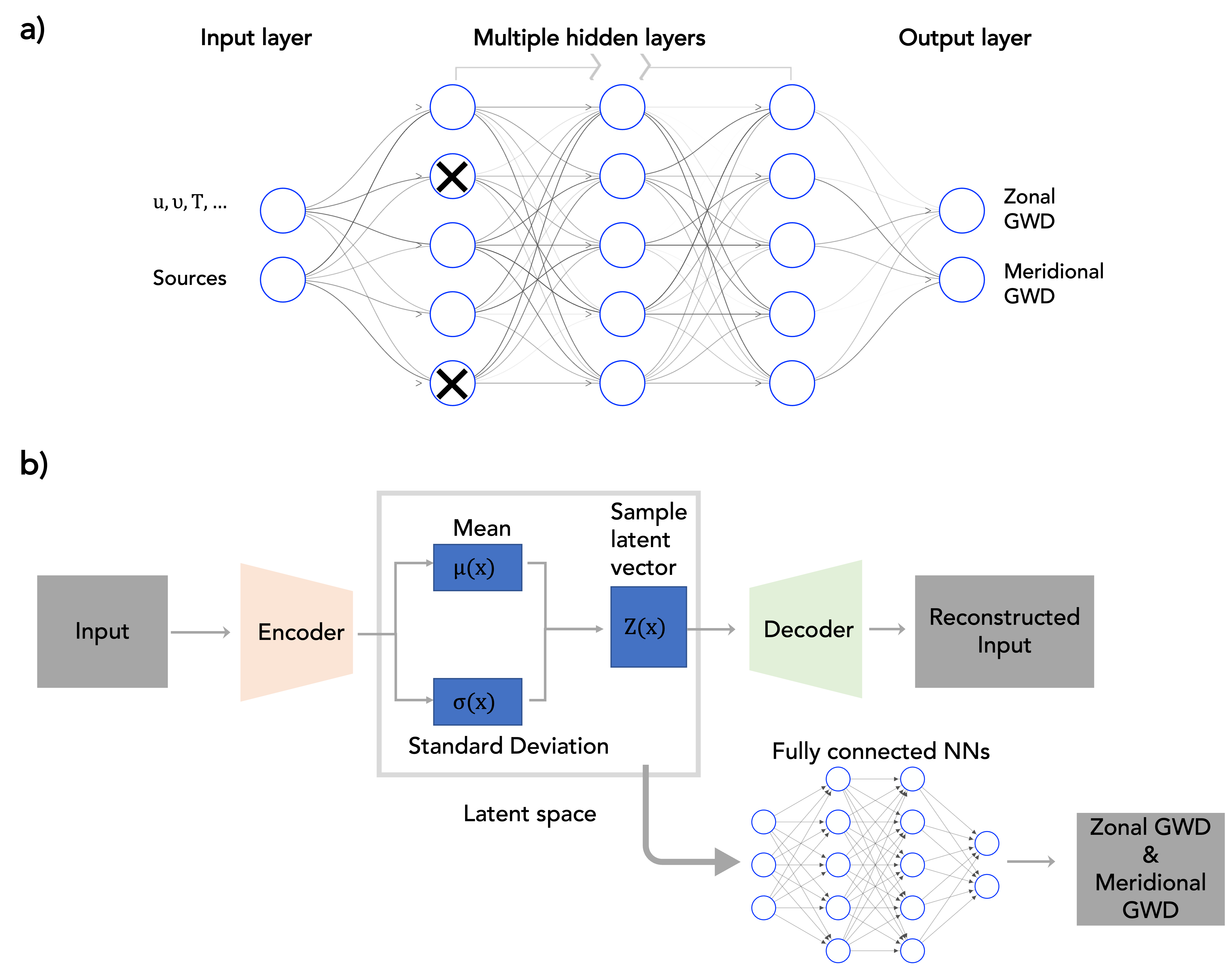
Here we briefly describe the general structure of the NN-based regression models trained as emulators for GWP schemes. For the deterministic artificial NN, denoted as ANN in this study, we use multilayer perceptrons (MLP). MLPs, which are feedforward fully connected NNs, take inputs through successive layers of linear transformation and non-linear activation functions to produce an output, so as to learn a functional relationship between the input and output (Figure 2a). Deep MLPs have multiple layers of weights, which are optimized over many samples of input-output data pairs. Such MLPs are thus very powerful in terms of learning complicated functional relationships. Generally, we can write the governing equations of an MLP as
| (1) |
where is the activation (output) of layer , is the weight matrix connecting layers and , and is the bias at layer , which allows the network to fit the data even when all input features are equal to 0. is the non-linear activation function.
In this study, we employ the same NN structure while training three distinct NNs, each for GWP originating from one of the three unique GW sources. The input layer contains the same input variables (see A) used by the WACCM GWPs across all vertical levels. There are 10 hidden layers in total (Figure 2a), and there are neurons in each hidden layer. In the output layer, both zonal and meridional GWD are predicted. The activation function in each layer, , is chosen to be swish (Ramachandran \BOthers., \APACyear2017), except for the output layer, where it is linear. During training, and are randomly initialized and learned by minimizing a loss function using an ADAM optimizer, with a fixed learning rate of . One of the loss functions used here is the common MSE, i.e.,
| (2) |
Here, is the number of training samples and is the norm. For training sample , vector contains all the inputs to the NN (A), vector contains the true zonal and meridional GWD at each vertical level, and denotes the trainable parameters, i.e., the weights ().
2.2.2 The UQ Methods and Metrics
Although deterministic NNs are powerfully expressive and can exhibit high out-of-sample predictive skills, they do not provide estimates of the uncertainty associated with their predictions. As mentioned earlier, currently there is no rigorous method to estimate the uncertainty of an NN prediction. That said, a variety of techniques have been developed for UQ in NNs, though the validity and usefulness of the estimated uncertainty for scientific applications remain subjects of ongoing investigations (e.g., Psaros \BOthers., \APACyear2023; Haynes \BOthers., \APACyear2023). In this paper, we use three different and widely used approaches to perform UQ from the ML literature: Bayesian neural network (BNN), dropout neural network (DNN), and variational auto-encoder (VAE). A brief overview of these approaches is provided below.
Bayesian neural network (BNN): A BNN combines the deterministic NN described earlier and in Figure 2a with Bayesian inference (Blundell \BOthers., \APACyear2015). Simply speaking, a BNN estimates distributions of the weights, rather than point values (as in a deterministic NN). The posterior distributions in the BNN (i.e., the distributions of the weights and biases) are calculated using the Bayes rule. In this study, we follow the standard practice and assume that all variational forms of the posterior are normal distributions. Furthermore, to accelerate the training process, we use the normal distribution for all the priors in the BNN (where is obtained from parameters of the trained deterministic NN). Note that while we are assuming normal distributions for the trainable parameters, the predictions generated by BNN can fit different distributions due to the use of nonlinear activation functions. The resulting distribution of the predictions during inference gives an estimate of their uncertainty.
Dropout neural network (DNN): A DNN is developed by randomly eliminating all outgoing connections from some of the nodes (Figure 2a) in each hidden layer of a deterministic NN during the training and the inference (Srivastava \BOthers., \APACyear2014). The fraction of nodes “dropped” on average in each layer is called the dropout ratio. Mathematically, Equation (1) can be reformulated for a DNN as:
| (3) |
where the dropout matrix is a square diagonal binary matrix of integers 0 or 1. The diagonal elements of follow a Bernoulli distribution where the probability of zero is the dropout ratio.
Dropout was initially developed as a regularization technique to prevent over-fitting in NNs. However, Gal \BBA Ghahramani (\APACyear2016) showed that training a NN with the dropout technique approximates a Bayesian NN. In this study, we use a dropout rate of 0.1, which is incorporated in all hidden layers, but we also investigate the sensitivity of the DNN to different dropout rates, as later shown in B. Note that the random dropping out is also used during inference, leading to a distribution for each prediction.
Variational auto-encoder (VAE): A typical VAE (Kingma \BBA Welling, \APACyear2014) consists of two NNs (Figure 2b): an encoder that transforms the input into a lower-dimensional latent space, parameterized by a normal probability distribution, and a decoder that inverts this transformation and produces the original input. The difference between the decoder’s output and the original input drives the learning process of the encoder and decoder, while the parameterized lower-dimensional latent space provides the uncertainty of this transformation. The VAE was developed for generative reconstructions of data by simply drawing samples from the latent space. The VAE is basically a dimension-reduction method. Many variants, however, have been proposed for more specific purposes. In this study, following Foster \BOthers. (\APACyear2021), we add a third NN, as illustrated in Figure 2b, that randomly draws samples from the parameterized latent space as inputs, and predicts the zonal and meridional GWDs as outputs. The difference between the predicted GWDs and the true GWDs drives the learning of the third NN. Consequently, the loss for the entire network consists of three components: the loss between the reconstructed input and the original input, the Kullback–Leibler (KL) divergence between the distribution of the latent space and a normal distribution, and the loss between the predicted GWDs by the third NN and the true GWDs.
For a specific input, each of these three UQ methods discussed above can be run multiple times, generating an ensemble of predictions with different realizations of the weights by drawing from the trained distribution. This is in contrast to the deterministic NN that provides just a single-valued prediction for a given input. These ensembles can then be used to quantify the uncertainty associated with that prediction. We expect that the RMSE of the ensemble mean should exhibit approximately a 1-1 relationship with the ensemble spread (i.e., the standard deviation of the ensemble members). To investigate this relationship, we use the spread-skill plot (Delle Monache \BOthers., \APACyear2013). Detailed calculations behind the spread-skill plot can be found in C, where we also introduce two metrics: spread-skill reliability (SSREL) and overall spread-skill ratio (SSRAT), both of which summarize the information presented in the spread-skill plot.
2.3 Transfer Learning
Transfer learning refers to leveraging/reusing information (weights) from an already well-trained base NN to effectively build a new NN for a different system from which only a small amount of training data is available (Yosinski \BOthers., \APACyear2014; Tan \BOthers., \APACyear2018; Chattopadhyay, Subel\BCBL \BBA Hassanzadeh, \APACyear2020). For our purpose, which is improving OOD generalization to the warmer climate, the TL procedure is as follows. For any of the NNs described earlier (e.g., the one in Figure 2a), we train them from randomly initialized weights and biases with data from the control simulations. The NN will work well during inference for test samples from the control but not from future (warmer climate) simulations (as shown in the Results section). To address this, TL is applied wherein most of the NN’s weights are kept constant, and only one or two hidden layers are re-trained using a limited dataset from the future simulation. Although this small dataset is insufficient for training an entire NN from random initialization, careful and correct selection of hidden layers for re-training, as discussed in Subel \BOthers. (\APACyear2023), allows the development of an NN that accurately adapts to the new system, i.e., the future climate conditions.
Here, we re-train the NN-based emulator that was initially trained on the control data with new data from only 1 month (30 consecutive days) of integration (1.4% of 6 years simulation for the initial training) of WACCM model under future forcing (4CO2). We have explored different choices of layers to re-train with the same amount of new data and found that re-training the first hidden layer yields the best results, consistent with Subel \BOthers. (\APACyear2023). Therefore, the results with only re-training the first hidden layer are shown in Section 3 unless stated otherwise.
3 Results
3.1 Data Imbalance
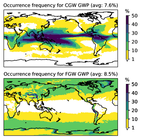
As discussed earlier, the physics-based GWP schemes in WACCM are directly linked to their sources. This means they only produce non-zero values when their respective sources are active. For example, in a specific grid box, CGWs only register non-zero values when there is active convection within that box. The heterogeneous and sometimes intermittent nature of these sources leads to a dataset that is significantly imbalanced. Figure 3 shows global maps of the occurrence frequency of non-zero GWD for CGWs and FGWs. On average, only of all GCM columns yield non-zero CGWs, primarily located in the tropics. Similarly, for FGWs, only of all columns have non-zero outputs, but unlike CGWs, the majority of these are located in mid-to-high latitudes, particularly along the storm track region. For the OGWs in WACCM, data imbalance presents a greater challenge, to be discussed in a later section. While it is possible to simply separate zero and non-zero columns for emulation work where we know the truth, this approach falls short with real-world data, which is the main purpose of this study.
In addition to their sources, several other factors specific to GWD data exacerbate the data imbalance problem. In the case of each GCM column with non-zero GW activity, momentum fluxes are generally concentrated at a few critical height levels rather than being smoothly distributed throughout the entire column. This further restricts the effective occurrence frequency of non-zero values. Moreover, GWs exhibit significant intermittency, where a small portion of large-amplitude GWs often dominates the morphology of the observed global GW momentum flux distribution (Hertzog \BOthers., \APACyear2012; Geller \BOthers., \APACyear2013). Therefore, it is crucial for NNs to not only accurately identify the columns that produce GWDs but also to effectively learn and recognize rare and extreme GWDs.
Given the complexity of the GWD dataset, different normalization methods are considered in this study. The first method, dubbed “NORM1”, is the typical normalization used in ML practices, which calculates elemental means and standard deviations for each feature (i.e., input variable at a given model level) and normalizes both inputs and outputs by these values (e.g., Espinosa \BOthers. (\APACyear2022)). With this approach, the same relative changes in wind at each level are treated equally in the input. The loss function in Equation (2) also penalizes the same relative error in GWD at each level equally. The second method, referred to as “NORM2“, is designed with the physics of GWD in mind. For the velocity inputs () and the tendency outputs (GWD), each column is normalized by one single value, which is the largest standard deviation from all model levels. Additionally, the mean values for these variables, are retained (e.g., ). Unlike NORM1, the original wind profile’s structure is preserved in NORM2, and large GWD values at certain heights maintain a relatively larger value after this normalization. For all other input variables, NORM2 is identical to NORM1. Compared to NORM1, NORM2 places more emphasis on large GWD values and penalizes the NN more for missing these significant tendencies. These two normalization methods are also employed in Chantry \BOthers. (\APACyear2021), who found similar performance from these methods with the non-orographic GWPs.
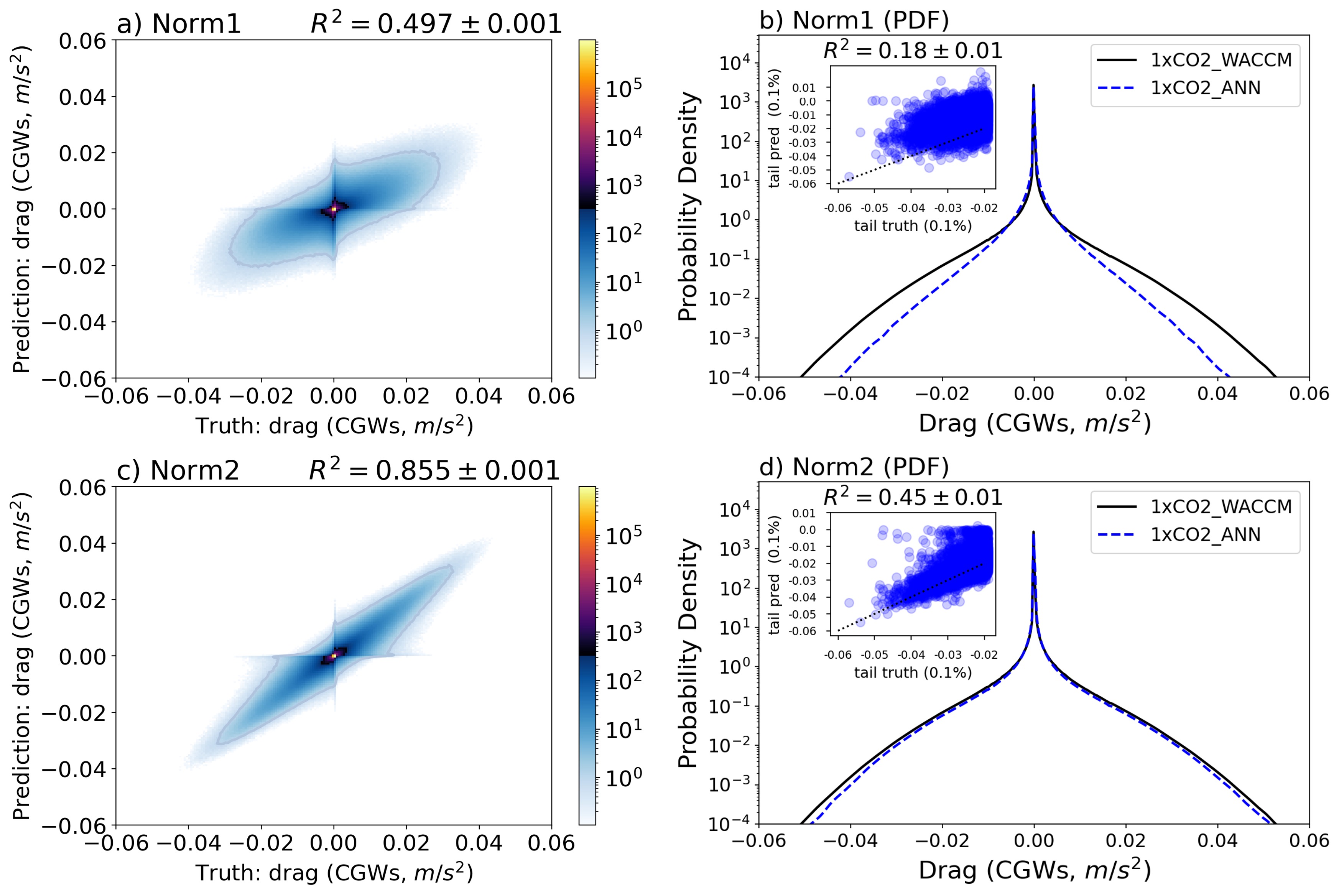
Figure 4 shows the performance of the emulations for CGWs with the two normalization methods. When employing NORM1, the conventional approach seen in prior ML practices, and also our initial attempts, the emulator’s performance is poor. Although the NN demonstrates some skill, its predictions tend to cluster around zero. However, when the second normalization method (NORM2) is employed, the emulation results show significant improvement, in contrast to the findings of Chantry \BOthers. (\APACyear2021). We attribute this improvement to the more pronounced data imbalance in our dataset, and it is likely a consequence of NORM2’s emphasis on modeling the large GWD values. Nonetheless, emulating the tail of the probability density function (PDF) (rare events) remains poor, as evidenced by the tails in Figure 4c, primarily due to the predominance of zero GWD columns in the training dataset. To more effectively address the data imbalance issue in these regression tasks, we further propose two approaches here:
-
1.
Resampling the data (ReSAM): In this approach, we limit the number of training sample pairs with zero GWD to be equal to the number of samples with non-zero GWD. This significantly reduces the number of columns with zero GWD, thus mitigating the data imbalance issue. Additionally, this sub-sampling reduces the total size of the training dataset, which, in turn, enhances the training speed (approximately sevenfold). While resampling methods have been well-established in the ML literature, they have mainly been used for classification problems. Their application to regression problems in climate research has not been extensively explored.
-
2.
Weighted loss function (WeLoss): Instead of assigning the same weight to all sample pairs in the loss function, we modify the weight for each column based on the PDF of its maximum GWD amplitude. This adjustment allows us to re-formulate the loss function defined in Equation (2) as
(4) where
(5) Note that, in practice, we lack knowledge of the precise PDF for the maximum GWD within each column. Therefore, we employ a histogram with 20 bins as an alternative. Given the fact that large-amplitude GW events are rare, the WeLoss approach incentivizes the NN to prioritize these significant events.
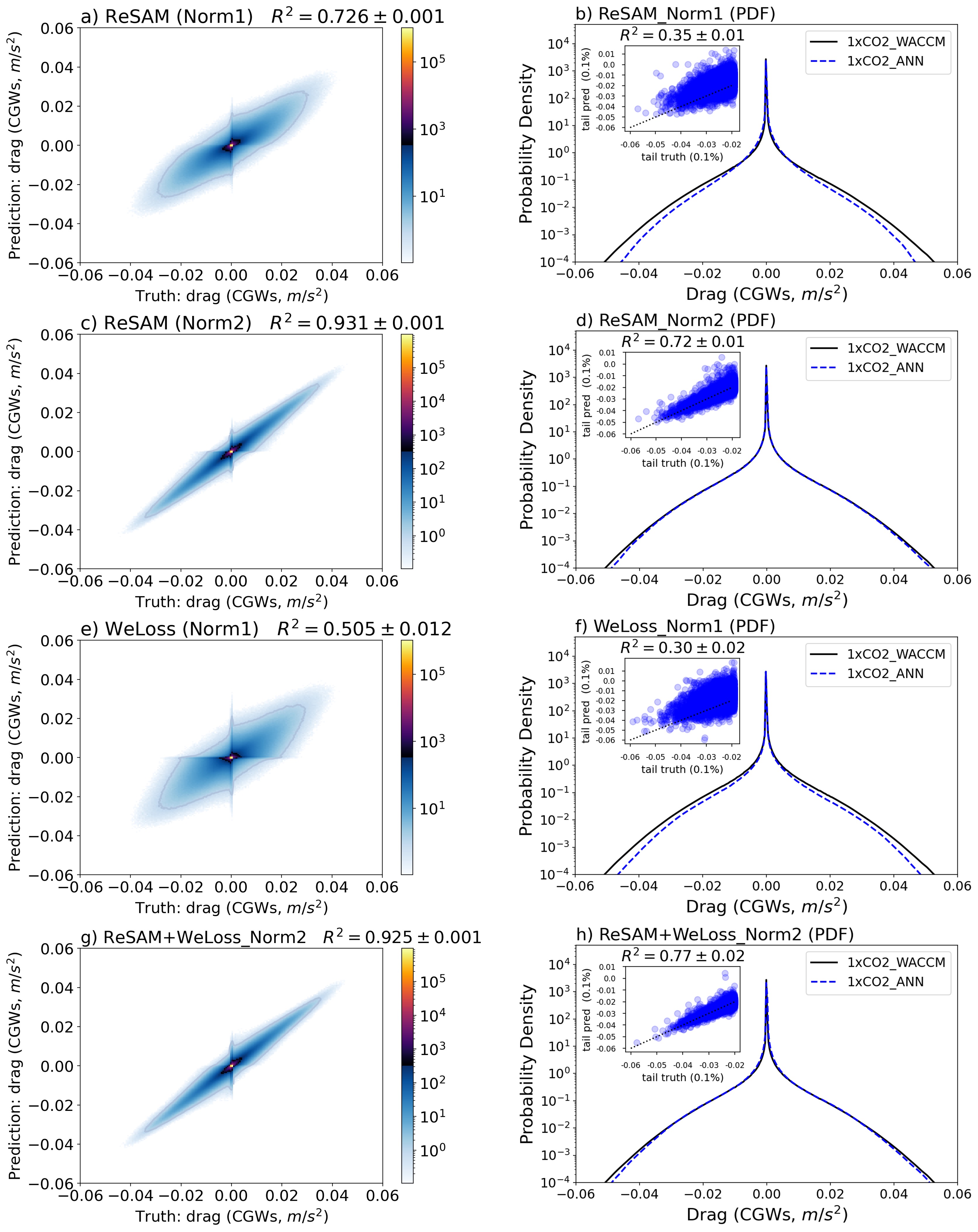
When we apply the ReSAM approach to balance the training dataset (after normalization with NORM1 or NORM2), the emulation results significantly improve, as shown in Figure 5. In fact, when considering the R-squared value between the NN prediction and the ground truth, the ReSAM approach with NORM2 yields the best results. However, as the training dataset is still predominantly composed of zeros and small GWD values due to the intermittence of the GWs, examining the emulation results for only large amplitude GW events (e.g., the top 0.1% in Figure 5d) reveals less satisfactory performance (). Regarding the WeLoss approach, it has a more limited impact on improving the R-squared value of the emulation (as shown in Figure 5e). However, it proves valuable in capturing the tails of the PDF and, thus, rare events (as depicted in Figure 5f). Moreover, as ReSAM and WeLoss represent distinct operations, they can be effectively combined when constructing a NN. The result of this combined approach for emulating the CGWs can be found in Figures 5g and 5h. While the R-squared value for the entire distribution only marginally changes (0.925 vs. 0.931 with ReSAM only), the performance of the emulation for the tail part has been improved ( increased to 0.77).
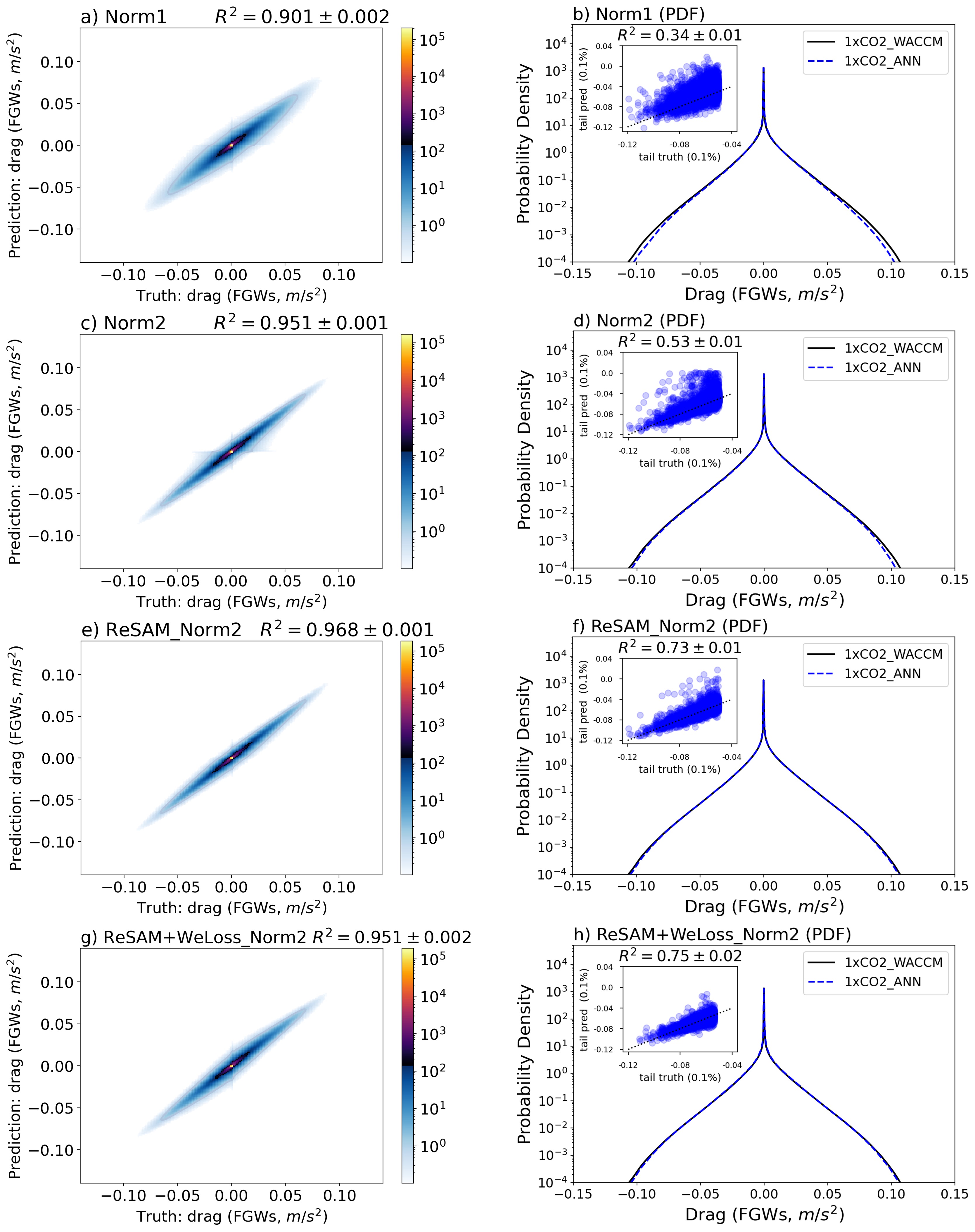
Similarly, Figure 6 presents the offline emulation results for the FGWs. The conclusions drawn for CGWs generally hold true. However, data imbalance in FGWs is less pronounced compared to CGWs, which simplifies the task of emulating FGWs. Even without any resampling or changes to the normalization or (see Figure 6a), we achieve reasonable emulation results (). One contributing factor is the wider spatial distribution of FGWs compared to CGWs (refer to Figure 3). Additionally, the source of FGWs (frontogenesis function) in WACCM exhibits a much more continuous nature compared to precipitation and diabatic heating. As the data imbalance issue is less severe for FGWs, the performance with different normalization methods becomes more similar, echoing findings from Chantry \BOthers. (\APACyear2021) who emulated non-orographic GWs (including convective and frontal GWs) together.
In summary, data imbalance can pose challenges when learning from data that closely resembles real-world data (further discussed in the subsequent section on emulating OGWs). Proper resampling techniques can significantly enhance the NNs’ performance by improving dataset balance. Furthermore, modifying the loss function to penalize the NNs more for missing extreme values can further improve performance at the tails of the PDF. For the remainder of the paper, unless otherwise specified, we continue to employ the ReSAM approach and the standard loss function with NORM2 unless stated otherwise.
3.2 Uncertainty Quantification
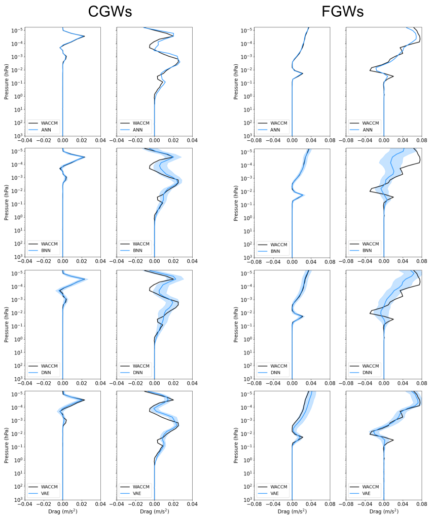
As outlined in subsection 2.2.2, we employ three different methods (i.e., BNN, DNN, and VAE) to quantify the uncertainty of predictions during inference (testing). For this purpose, an ensemble of 1000 members is generated by running each UQ-equipped NN 1000 times for each input from the testing set. Figure 7 presents sample profiles of zonal GWD derived from the deterministic NN (ANN) and the three UQ-equipped NNs, alongside the true GWD profiles from WACCM. Note that these examples have not been used in the training or validation process. It is evident from the figure that all three UQ-equipped NNs show reasonable skill in predicting the complex profiles of GWD due to CGWs and FGWs (also reflected in R-squared in Table 1), albeit with a slight decrease in accuracy compared to ANN. As discussed earlier, a valuable uncertainty estimate should correspond closely with the NN’s test accuracy, providing insights into when to trust the NN’s prediction during inference. Such a relationship can be seen in a few randomly chosen GWD profiles that’s shown in Figure 7. In each pair of CGW and FGW profiles, the left column shows the estimated uncertainty is also low when the prediction error is low, indicating the NN’s confidence in its accurate predictions. In contrast, the right column, which generally represents more complex profiles, exhibits the NN’s less accurate predictions, and increased uncertainty, highlighted by the wider confidence intervals.
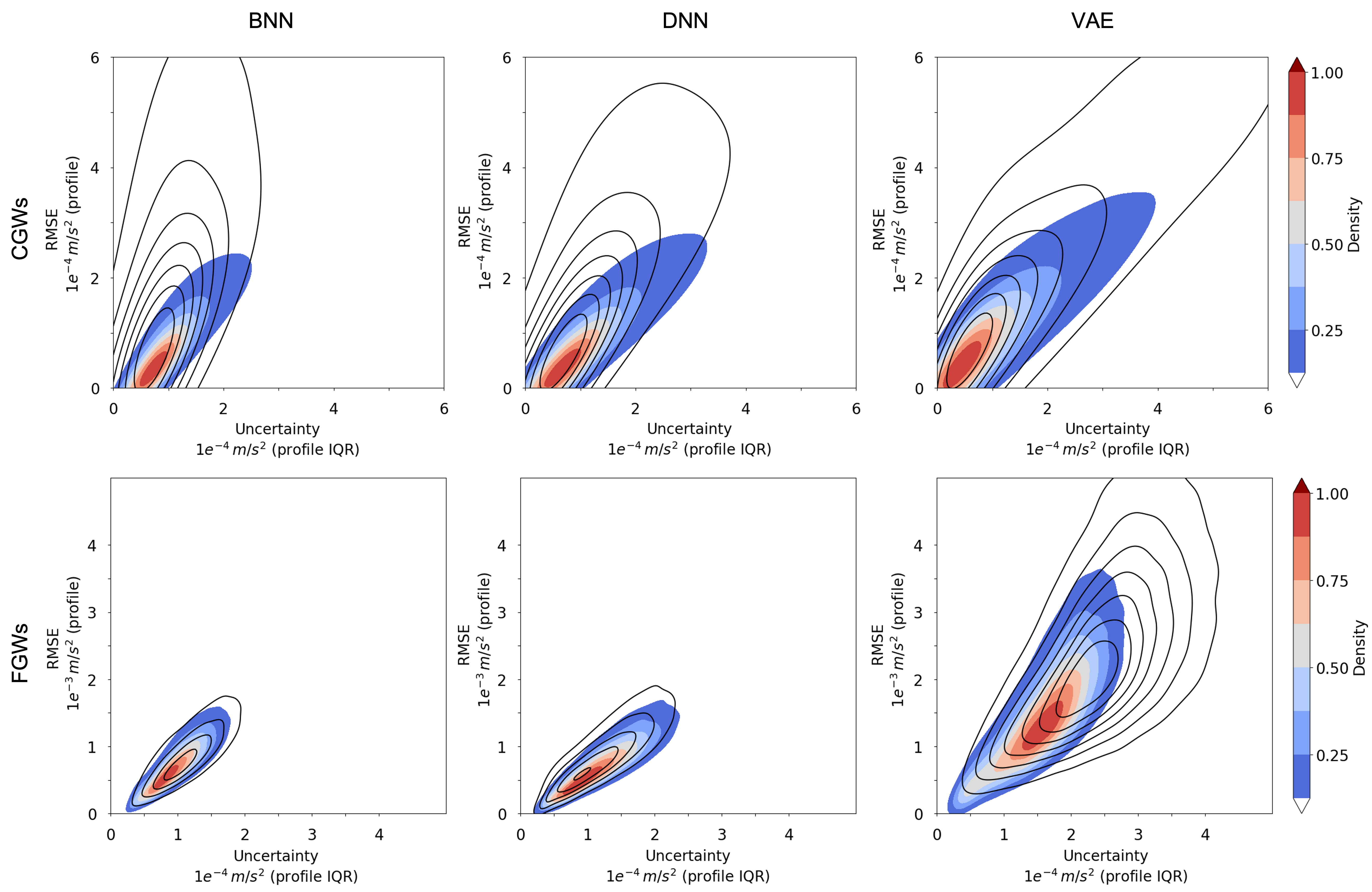
While Figure 7 demonstrates the performance of the UQ methods for just a few GWD profiles, the spread-skill plots shown in Figure 8 offer a broader perspective based on 60,000 profiles, following the calculations detailed in C. It is evident from the plots that all three UQ methods produce reasonably informative uncertainty estimates, as their curves closely align with the 1-to-1 line. In the case of CGWs, all data points are above the 1:1 line, indicating a slight overconfidence (underdispersiveness) across all three UQ methods, with the DNN being slightly closer to the 1-to-1 line. For the FGWs, the DNN demonstrates slightly better performance, although it marginally drops below the 1-to-1 line in the first few bins, indicating a slight underconfidence. Notably, it can be seen from the spread frequency inset that the vast majority of the data points are within the first few bins, for which both spread and skill values are small, and they are generally closer to the 1-to-1 line.
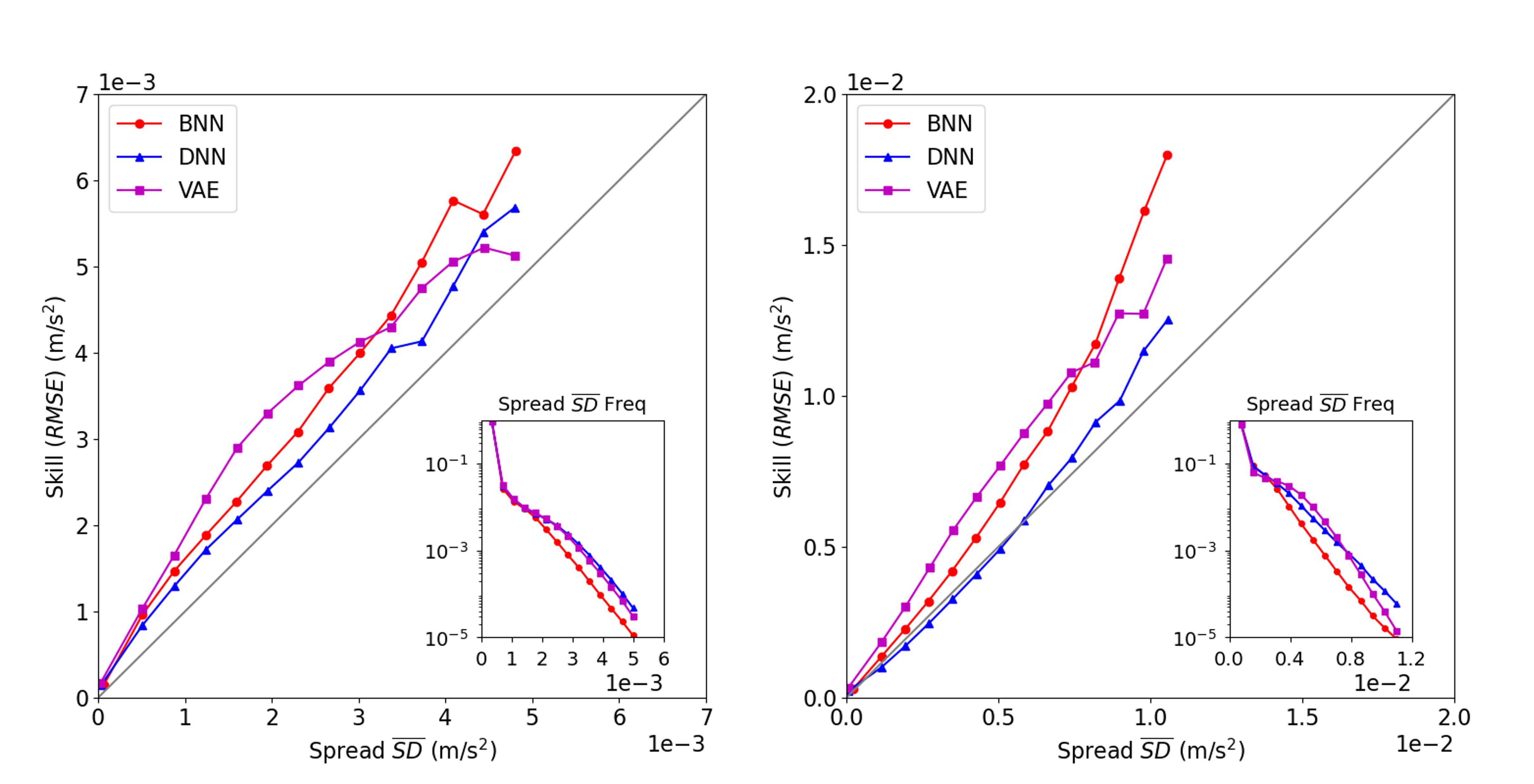
It should also be noted that for the large values of model spread (), there is only a very limited number of data points, as is evident from the inset histograms. Consequently, the standard deviation (STD) can become a misleading measure of spread because of the non-normal distributions.
To summarize the quality of the spread-skill plots for the three UQ methods, we explore the metrics introduced in subsection 2.2.2 and C (see Table 1). The R-squared value for the ensemble mean prediction is also given to show the accuracy of each UQ method. Based on SSREL, whose ideal value is zero, BNN shows the best performance for both CGWs and FGWs. However, if we check SSRAT, where 1 is the optimal number, DNN is the best among these three methods. This discrepancy can be explained by a closer look at the Equations (7) and (8). SSREL, which is a bin-weighted average difference, is most sensitive to the performance of the NN in the first bin, where the vast majority of the data points are located (see the inset histograms in Figure 8), while SSRAT is more influenced by larger values of spread and skill. Accordingly, the VAE shows the highest values of SSREL, which is indicative of its sub-optimal performance in the first bin, where there are small values of spread and skill.
In the results presented in Figure 8 and Table 1, each height level of a GWD profile is considered as an individual sample. A zonal GWD profile, with its 70 vertical levels, thus constitutes 70 distinct samples. While analyzing these samples offers insights into the NN’s overall performance by averaging statistics across numerous profiles, our primary interest is often in the uncertainty associated with an individual GWD profile. This uncertainty can then aid in determining whether to trust/use the NN’s prediction for that particular GWD profile. Therefore, we use Equation (9) to assess the relationship between uncertainty and test accuracy for each GWD profile. Furthermore, to estimate uncertainty, here we use the interquartile range (IQR) to reduce the influence of outliers.
Figure 9 shows the Gaussian kernel density of spread against RMSE for all 60,000 profiles, as indicated by the color shading. The -axis represents the IQR of each GWD profile, while the -axis denotes its corresponding RMSE. A strong correlation between the two is observed across all three UQ methods. Consequently, GWD profiles with larger uncertainties often coincide with larger errors. Figure 9 also shows a close similarity between BNN and DNN. In contrast, VAE tends to provide marginally larger uncertainties, especially for FGWs. This is consistent with VAE’s slightly reduced accuracy as indicated in Table 1. Overall, given the monotonic relationship between the uncertainty and test error, these results show that all three UQ methods provide useful and informative uncertainty for with-distribution test samples. A user can set a threshold on uncertainty based on their tolerance for error (RMSE) and decide whether they trust the NN for a given input sample.
The results presented so far show the performance of the UQ methods based on the testing data, i.e., data from the current climate. However, the effective performance of UQ methods can also be tested (perhaps more meaningfully) on OOD data, e.g., data from a warmer climate. This is particularly relevant for climate change studies. Accordingly, we evaluate the performance of these trained NNs with input data from the future climate, as depicted by the black lines in Figure 9. For FGWs, the spread-skill relationship remains largely similar, especially for BNN and DNN. This suggests that, based on their uncertainties, we can still reliably estimate the error in the NN predictions for FGWs for the warming climate. A similar pattern is observed for the VAE, though it exhibits increased uncertainties and higher errors with OOD data. As shown in a later section, for FGWs, the NNs generalize to the warmer climate without any further effort.
In contrast, for CGWs, given the same level of uncertainty, the error in NN predictions increases significantly for the OOD data compared to that from the current climate, which means the spread-skill relationship, especially for the BNN and DNN, fails to generalize to the OOD data. From this perspective, VAE performs better, showing that for the same level of uncertainty, the increase in error is not as substantial as in BNN and DNN. The VAE also yields considerably higher uncertainty estimates for future climate, which may aid in the detection of OOD data. The observed discrepancies in the performance of the NNs for CGWs and FGWs hint at different levels of their generalizability, a topic we will delve into more deeply in the following subsection.
| CGWs | FGWs | |||||
| BNN | DNN | VAE | BNN | DNN | VAE | |
| SSREL (1e-4) | 1.29 | 1.48 | 2.14 | 1.20 | 1.69 | 5.21 |
| SSRAT | 0.73 | 0.82 | 0.72 | 0.69 | 0.93 | 0.69 |
| R-squared | 0.90 | 0.86 | 0.87 | 0.94 | 0.92 | 0.89 |
In summary, while the three UQ methods provide credible and valuable uncertainty estimates for the current climate, the BNN and DNN are confidently wrong in estimating CGWs in a warmer climate although VAE shows some promising results. This problem is common among various UQ techniques as pointed out in the ML literature: they frequently show overconfidence when assessed with OOD data (e.g., Ovadia \BOthers., \APACyear2019). The optimal UQ method selection depends on the specific metric of interest and the intended application. While BNN is more broadly used in the literature and gives the best accuracy, DNN could achieve similar performance and is often more practical given its simplicity. On the other hand, VAE seems to perform better when applied to OOD data, at least in the one test case here. These observations warrant further research in the future using multiple test cases and climate-relevant applications. We also note here that each method has multiple tuning hyperparameters to optimize its uncertainty quantification. Consequently, the discrepancies among the three methods could potentially be mitigated with proper hyperparameter tuning (as discussed in B).
3.3 Out-of-distribution (OOD) Generalization via Transfer Learning
As previously discussed, the GWP schemes in WACCM are coupled to their sources, which might change in a warmer climate. Specifically, under CO2 forcing, we expect changes in both the amplitude and the phase speed distribution of GWs, in particular for the CGWs, due to their built-in sensitivities to changes in the convection. Consequently, the physics scheme in WACCM produces slightly stronger GWD for CGWs, especially in the tail of the distribution. This intensified GWD results in a shorter quasi-biennial oscillation (QBO) period in WACCM. However, it is important to recognize that the response of the QBO to climate change differs across various general circulation models (Richter \BOthers., \APACyear2022).
The intensification of the CGWs in future climate simulations presents an opportunity to study how NNs handle the OOD data. Our findings in the UQ section already suggest increased prediction errors when testing NNs with OOD data, which raises concerns about their applicability in climate change studies. To more thoroughly investigate this issue, we conduct additional evaluations on our ANNs, by applying them to data samples from future climate simulations, as illustrated in Figure 10. It is clear that the ANN for the CGWs does not generalize well, evidenced by a decrease in from 0.93 to 0.79. The ANN particularly struggles to capture the increase in GWD in the tail, with for the tails decreasing from 0.72 to 0.36. As a result, it seems unlikely that this emulator will accurately reproduce changes in the circulation under different climate conditions, such as the shorter QBO period resulting from future warming in WACCM.
In contrast to CGWs, the amplitude of FGWs shows a less marked increase in the future climate, and their PDF distribution closely resembles that of the control simulations. As a result, the ANN demonstrates better generalizability for FGWs when it is tested against future climate data, as seen in Figure 10d. There is only a slight decrease in the ANN’s performance, with dropping from 0.97 to 0.95.
Two factors can contribute to the considerable OOD generalization errors in an NN when applied across two distinct systems. First, the input-output relationship might vary between the two systems. Second, the input variables in the new system could originate from a distribution different from that of the original system (regardless of whether the input-output relationship remains the same or changes). The former is hard to quantify in a high-dimensional dataset. The latter can be quantified using similarity distances. To help us better understand these differences between the OOD generalizability of CGWs and FGWs, we assess the similarity between their input and output data distributions from control and future climate simulations using the Mahalanobis distance (). The Mahalanobis distance is a measure of the distance between a data point and a distribution (Ling \BBA Templeton, \APACyear2015). Specifically, it is a multi-dimensional generalization of the idea of measuring how many standard deviations away a point is from the mean of the distribution. The application of Mahalanobis distance in understanding the source of OOD generalization errors in data-driven parameterization was previously demonstrated in Guan \BOthers. (\APACyear2022) for a simple turbulent system.
| Variables | Source (diabatic heating for CGWs, frontogenesis for FGWs) | Zonal drag | Meridional drag | |||
| Distance (Convection) | 1.03 | 1.00 | 1.19 | 3.62 | 1.42 | 1.44 |
| Distance (Front) | 1.03 | 0.96 | 1.50 | 1.10 | 1.00 | 1.00 |
To use the Mahalanobis distance, we first calculate the mean and covariance matrix of the training data from the control run. We then analyze the distribution of Mahalanobis distances in this training data, setting a baseline value, referred to as . This baseline is the average distance for data points that deviate by more than 3 standard deviations from the mean. This choice aims to focus on outliers for which extrapolation is more challenging. Following this, we apply the same process to the data points in the future climate dataset, denoted as . Table 2 presents the ratio of for the warming scenario to for the control scenario for selected variables. When this ratio is close to 1.0, it suggests minimal changes in this variable’s distribution under a warming scenario. Note that the NNs trained based only on these variables demonstrate performance comparable to NNs trained on all variables (not shown), which is why we only focus on these few key variables.
The results reveal that among the various variables significantly contributing to the emulation of CGWs, diabatic heating (source of CGWs) is the sole variable that exhibits substantial changes from the control to the warming scenario. Conversely, changes in variables used to emulate FGWs are considerably smaller. This outcome suggests that the likely reason for the better generalizability of FGWs is that the input distribution remains almost unchanged (and the input-output relationship, which is the physics scheme, remains the same too).
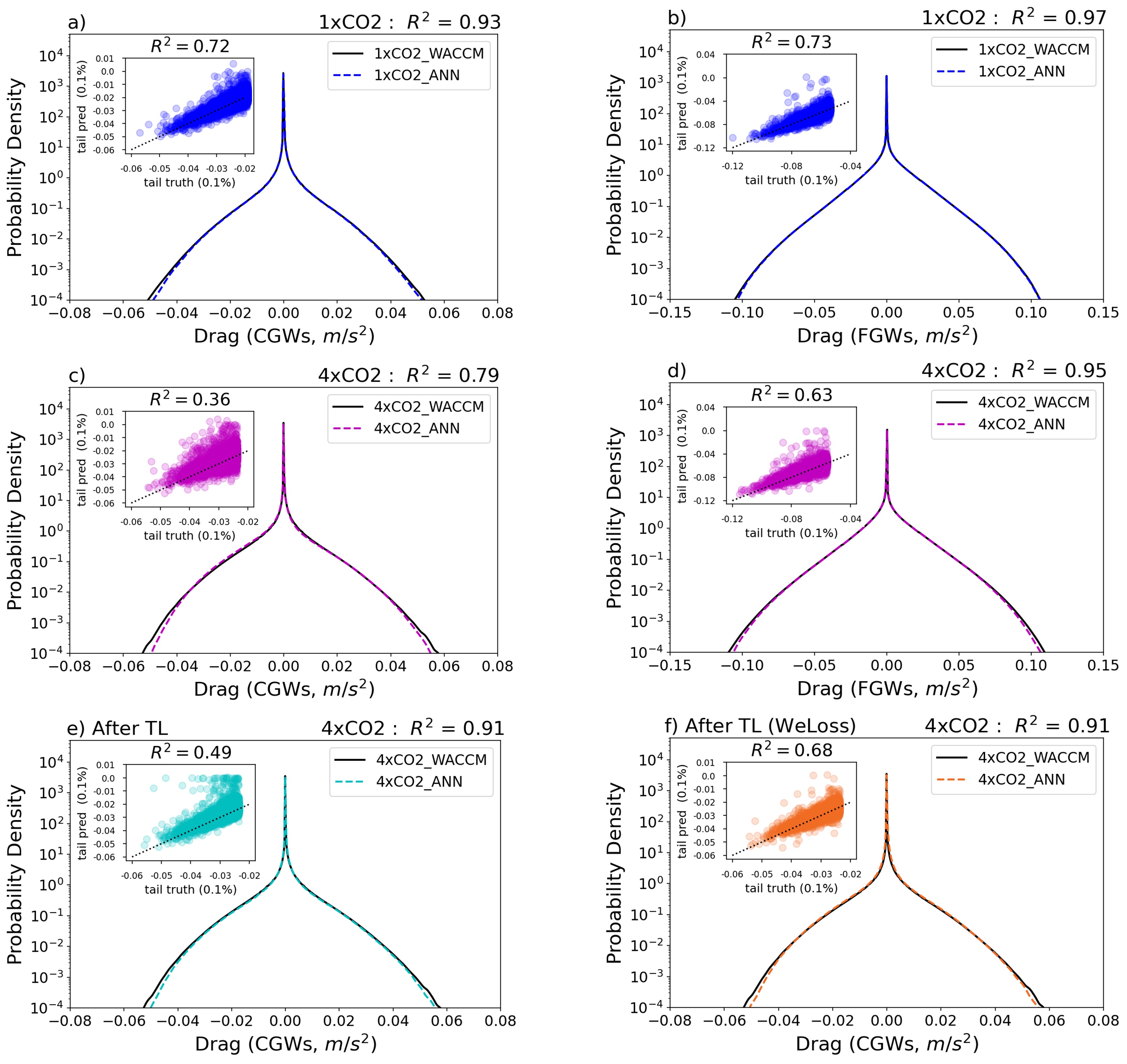
To improve the generalizability of the emulator for CGWs, we explore TL, a technique introduced earlier and proven to be a powerful tool for improving the OOD generalizability of data-driven parameterization in canonical turbulent flows (e.g., Guan \BOthers., \APACyear2022; Subel \BOthers., \APACyear2023). Rather than re-training the entire NN for future climate scenarios, we only re-train, follwoing Subel \BOthers. (\APACyear2023), just a portion of the NN, thereby requiring only a small fraction of the data. Figure 10e showcases the emulation results after only re-training the first hidden layer of ANN using data from the first month of the WACCM simulation in the CO2 scenario, which amounts to approximately 1% of the original training dataset. After applying TL, the performance of the emulator in the warming scenario significantly improves, with rising from 0.79 to 0.91, nearly matching its performance in the control simulations ( = 0.93). However, the improvement in the PDF tails is less pronounced, showing only a modest increase in from 0.36 to 0.51. This is likely due to the limited number of large-amplitude GW events within the one-month period. Instead of using more data from the future climate (which is challenging to obtain in a realistic situation), we leverage the WeLoss approach, described earlier, during re-training. This modification results in a significant improvement in the tail, with increasing from 0.51 to 0.68. Note that this improvement in the tail is critical, as inadequate learning of these rare but large-amplitude GWDs can result in significant errors and instabilities.
We would like to point out that during the TL experiments, we have examined the effects of re-training each individual hidden layer of the NN. Our findings indicate that re-training the first layer yields the best results, which aligns with the findings in Subel \BOthers. (\APACyear2023). Re-training the last layer only brings marginal improvements to the NN (not shown). Notably, our experiments involving re-training the first two layers did not result in further performance enhancements, suggesting that the number of neurons is not the primary factor contributing to the varied performance observed when re-training different layers.
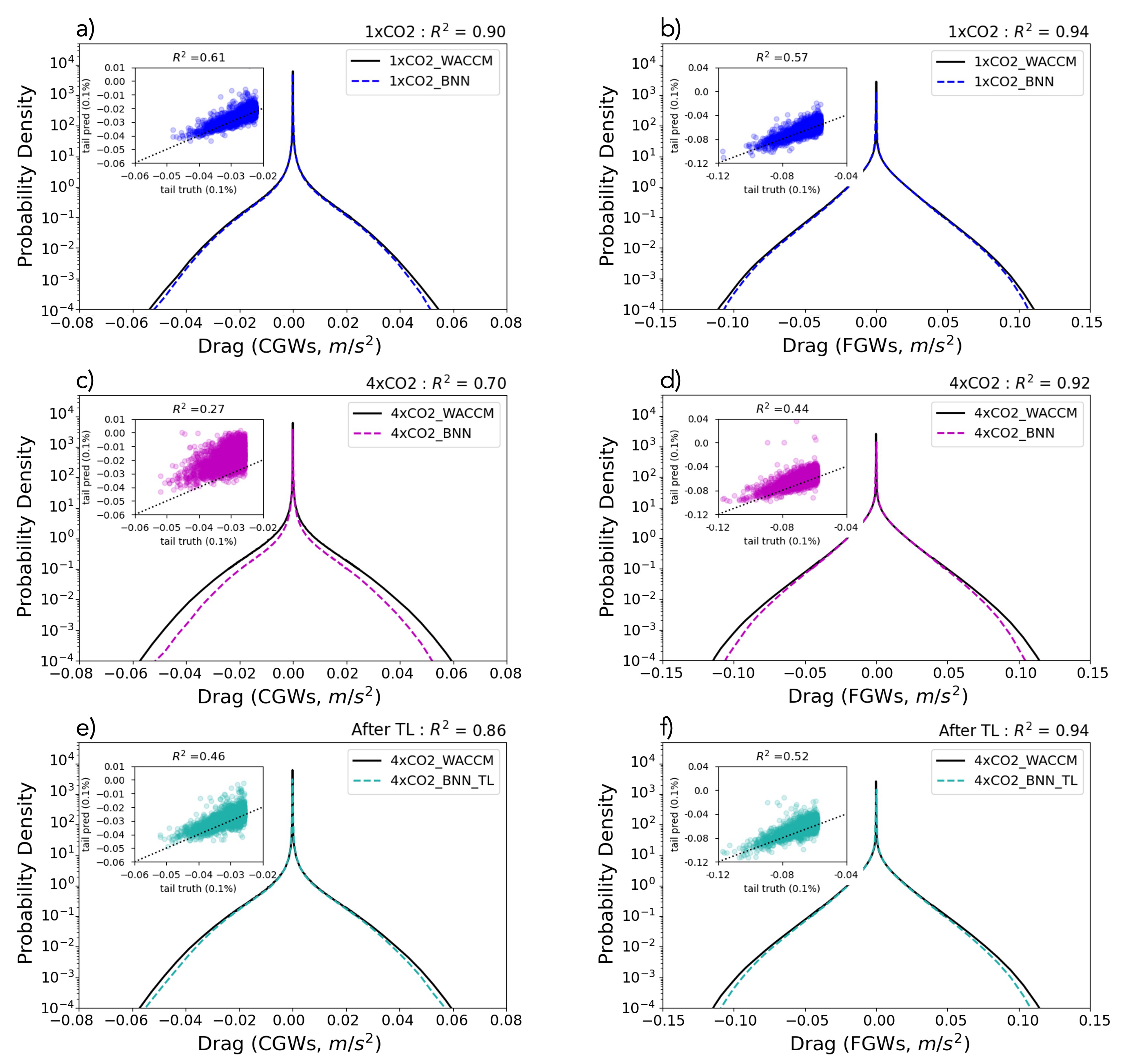
Similar results regarding TL are also observed with other NNs used in this study. For instance, Figure 11 presents the same plot as Figure 10, but for the BNN. It is evident that BNN also struggles with generalization to OOD data, as could also be interpreted based on the results presented in section 3.2. It is also the case for DNN and VAE (not shown). Overall, when these NNs are tested against the CO2 future climate data, their accuracy is not better than the deterministic ANN. However, methods with UQ, especially the VAE (see Figure 9), could potentially indicate the increased uncertainty when testing with input data from the CO2 integration. These results underscore the necessity of re-training the NNs using TL.
4 Emulation of Orographic GWs (OGWs)
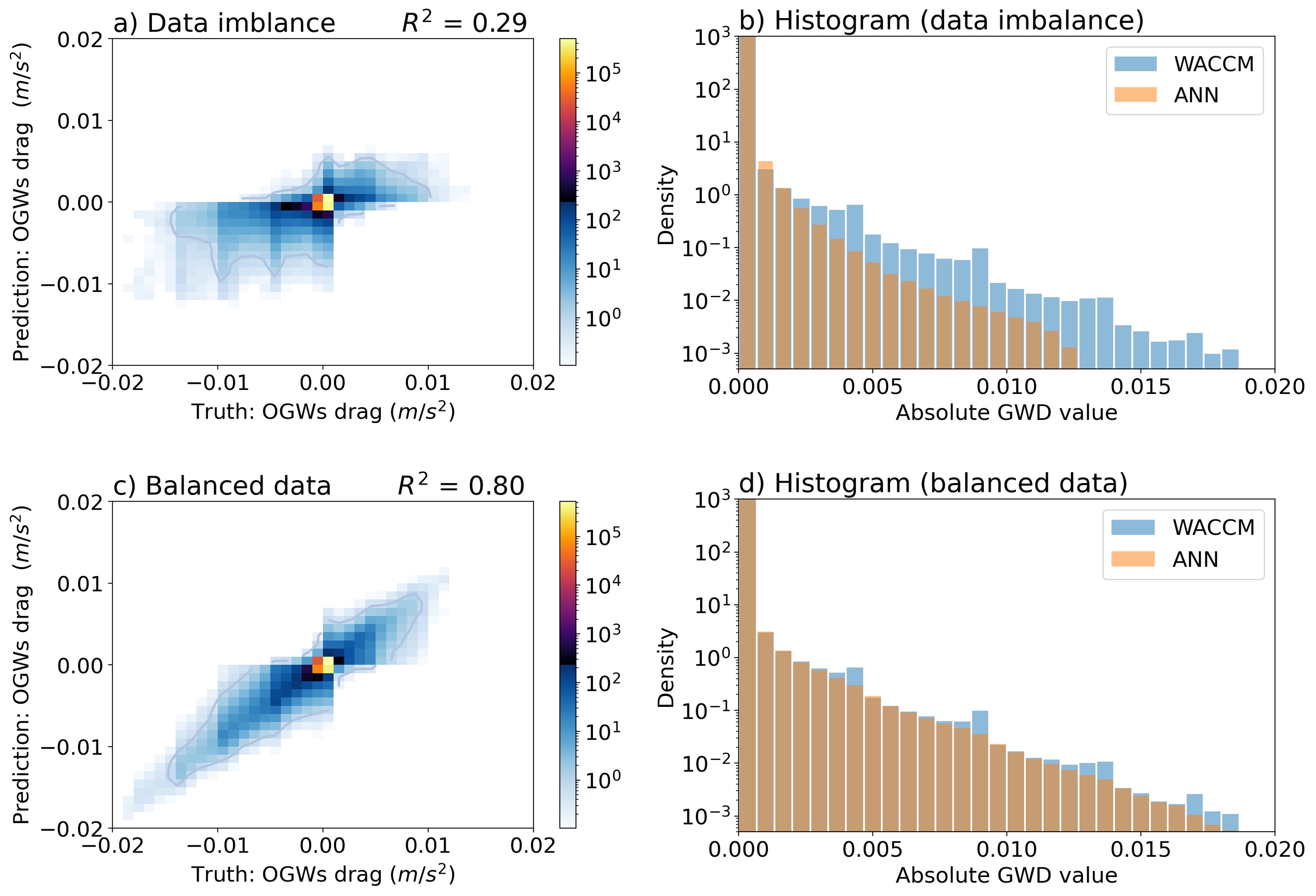
Similar to Chantry \BOthers. (\APACyear2021), our initial attempts to emulate OGWs did not succeed, primarily due to the presence of a pronounced data imbalance. Notably, the physics-based scheme responsible for OGW generation operates exclusively over terrestrial regions. However, it is surprising that the issue of data imbalance continues to persist, even when we limit our NN training and testing exclusively to columns located over land (Figure 12a). Still, the emulated OGW drag often remains close to zero and completely fails to predict the rare events (Figure 12b), which poses a considerable hurdle for the emulator’s performance. Further investigations reveal that the key to this problem lies in the highly localized nature of orographic GWD, where significant drag is observed only at a handful of specific locations. Furthermore, even within these limited regions, GWD exhibits a significant intermittent behavior. To help our understanding, we also conducted a -means clustering analysis, categorizing GWD data for all land-based columns (Table 3). Among the 6 clusters, cluster 4 accounts for a staggering of the dataset. Remarkably, all samples within this cluster exhibit exceptionally weak orographic GWD, as evidenced by the cluster center’s maximum GWD amplitude, which is two orders of magnitude smaller than that of other clusters.
| Cluster | Frequency (%) in the training data | Maximum GWD amplitude of cluster center |
| c1 | 0.18 | 8.7 e-3 m/s2 |
| c2 | 0.13 | 4.4 e-3 m/s2 |
| c3 | 0.93 | 3.6 e-3 m/s2 |
| c4 | 97.51 | 2.8 e-5 m/s2 |
| c5 | 0.15 | 2.1 e-3 m/s2 |
| c6 | 1.10 | 4.3 e-3 m/s2 |
To overcome this persistent data imbalance in the OGWs, we first separate all columns over land into large-drag columns (with column maximum greater than one STD of all GWD from OGWs) and small-drag columns. We then perform subsampling on the latter group only to create a more balanced dataset. To improve NN training, we also include all columns from the 6-year simulation to augment the sample size of the large-drag columns. Figures 12c and 12d illustrate the performance after re-balancing the dataset. Notably, the result represents a substantial improvement, evidenced by an increase from 0.29 to 0.80, and also a significant improvement in the accuracy for rare events. While we acknowledge that this skill remains lower than what is achieved for CGWs and FGWs, it already signifies a reasonable NN. Furthermore, we posit that by incorporating additional training data (either by extending the WACCM model integration or simply augmenting the data with OGWs scheme only), we can further improve our emulation results. The possibility of achieving superior emulation outcomes through the adoption of an alternative NN architecture is also possible, although such exploration is beyond the scope of this paper.
5 Summary and Discussion
Through the emulation of complex GWPs in a state-of-the-art atmospheric model (WACCM), we have elucidated and explored solutions for three critical challenges in the development of ML-based data-driven SGS schemes for climate applications: data imbalance, UQ, and OOD generalizability under different climates. A brief summary is provided below:
-
1.
In the presence of non-stationary, and highly imbalanced datasets, such as those encountered in WACCM, specialized approaches (e.g., resampling and weighted loss function) are essential to enhance the performance of data-driven models. Through resampling, we have successfully trained a robust NN emulator for OGWs, a challenging task as demonstrated in Chantry \BOthers. (\APACyear2021). The effectiveness of the trained emulator is also significantly influenced by the choice of the loss function used during training. In our case, while a weighted loss function (WeLoss) does not improve the overall score, it yields significant improvements in the emulation results for the PDF tails of the GWD. This finding aligns with those in Lopez-Gomez \BOthers. (\APACyear2022), where their custom loss function, tailored to emphasize extreme events, led to substantial improvements in predicting heatwaves.
-
2.
All three UQ methods employed in this study provide reasonable uncertainty estimates for GWD prediction for the current climate. The spread-skill plots (refer to Figures 8 and 9) indicate that greater uncertainty corresponds to a larger prediction error. Yet, the reliability of UQ methods diminishes when they are challenged with OOD data. Both BNN and DNN used in this study tend to be overconfident in estimating CGWs in a warmer climate, thereby struggling to identify OOD samples. The VAE, on the other hand, yields rather promising results in providing useful UQ for OOD data. Given the variations in different methods, the metrics selected to assess the SGS model will play a significant role in determining the choice for the UQ methods. We also note that further optimization of tunable parameters within each UQ method could affect their performance (refer to C).
-
3.
Our findings illustrate the challenges SGS schemes face in generalizing to OOD data and extrapolating to new climates. Nonetheless, the TL approach has proven highly effective in aiding an NN to extrapolate to different climates. For CGWs in WACCM, the physics-based scheme exhibits larger GWD under CO2 forcing, primarily due to an increase in diabatic heating from convection. With only one month of simulation data from this future warming scenario (representing approximately 1% of the original training dataset), we successfully reduce its OOD generalization error through re-training the first layer of the NN, following the findings of Subel \BOthers. (\APACyear2023). Additionally, we have illustrated the value of metrics like the Mahalanobis distance in assessing the potential OOD generalizability of NNs.
We would like to emphasize that these challenges are often intertwined. For instance, addressing data imbalance in CGWs is a prerequisite for obtaining an accurate NN model, which, in turn, impacts UQ and OOD generalizability assessments. Moreover, there exists a strong link between UQ and OOD generalizability evaluations: if the NN struggles with OOD generalization, performing poorly with OOD data, the reliability of UQ for such data (e.g., data from a warmer climate) also becomes questionable. This presents a substantial challenge for UQ methods, especially for climate change research where reliable UQ methods are crucial.
This study has primarily focused on offline skill assessment. We acknowledge that good offline performance (at least in terms of common metrics such as ) is not necessarily an indicator of stable and accurate online (coupled to climate model) performance (Ross \BOthers., \APACyear2022; Guan \BOthers., \APACyear2022), though more strict metrics such as of the PDF tails might better connect the offline and online performance (Pahlavan \BOthers., \APACyear2023). However, for the purpose of this study, which is to provide a testbed to test ideas for data imbalance, UQ, and OOD generalization with transfer learning, the offline tests, particularly using the several metrics we have used, suffice. That said, the main reason that we have not provided online results is that coupling various complex NNs, with the same framework, to complex climate models (e.g., WACCM) without slowing down the model is a challenging and time-consuming task (Espinosa \BOthers., \APACyear2022), and this is work in progress.
Emulating complex GWPs within the WACCM provided a unique opportunity to address three critical challenges in developing ML-based, data-driven SGS schemes for climate science applications. However, it is crucial to acknowledge that such emulated schemes essentially adopt the limitations inherent in the physics-based schemes. Addressing these limitations, the next step is to harness high-resolution data from GW-resolving simulations, which are carefully validated against observational data. A library of such high-resolution simulations, notably of convectively generated GWs using the Weather Research and Forecasting (WRF) model, is now established (Y\BPBIQ. Sun \BOthers., \APACyear2023), alongside additional global high-resolution simulations (Wedi \BOthers., \APACyear2020; Polichtchouk \BOthers., \APACyear2023; Köhler \BOthers., \APACyear2023). The next phase involves integrating the approaches outlined in this study with the data from these GW-resolving simulations to develop a stable, trustworthy, and generalizable data-driven GWP scheme. This scheme is then expected to overcome the limitations of physics-based GWPs and potentially incorporate features like the transient effect (Bölöni \BOthers., \APACyear2021; Kim \BOthers., \APACyear2021) and lateral propagation of GWs (e.g., Sato \BOthers., \APACyear2009)—marking a significant advancement towards next-generation GWP schemes.
Appendix A Input/output variables for the physics-based GWP schemes and their emulators
We use the exact same inputs as those of each GWP scheme in the WACCM for the training of the NN-based emulator of that scheme. These inputs are listed in Table 4. As for the outputs, we only consider the zonal and meridional drag forcings. The GWPs in WACCM also estimate additional effects of the GWs that result in changes of temperature profile and vertical diffusion. These outputs are not considered in our emulations.
| GWP | Input | Output | ||
| pressure levels | surface level | forcing | ||
| CGWs | Brunt–Väisälä frequency (70), dry static energy (70) | lat (1), lon (1), (1), | diabatic heating (70) | zonal drag GWDx (70), meridional drag GWDy (70), |
| FGWs | frontogenesis function (70) | |||
| OGWs | mxdis (16), hwdth (16), clngt (16), angll (16), anixy (16), | |||
From Table 4, one can guess that some input variables are correlated with each other. Consequently, it is plausible that the trained NNs may have spurious connections. Preliminary tests further support this notion, indicating that employing only and the forcing function as inputs yields comparable offline skill (results not presented here).
Appendix B Tuning UQ-equipped NNs
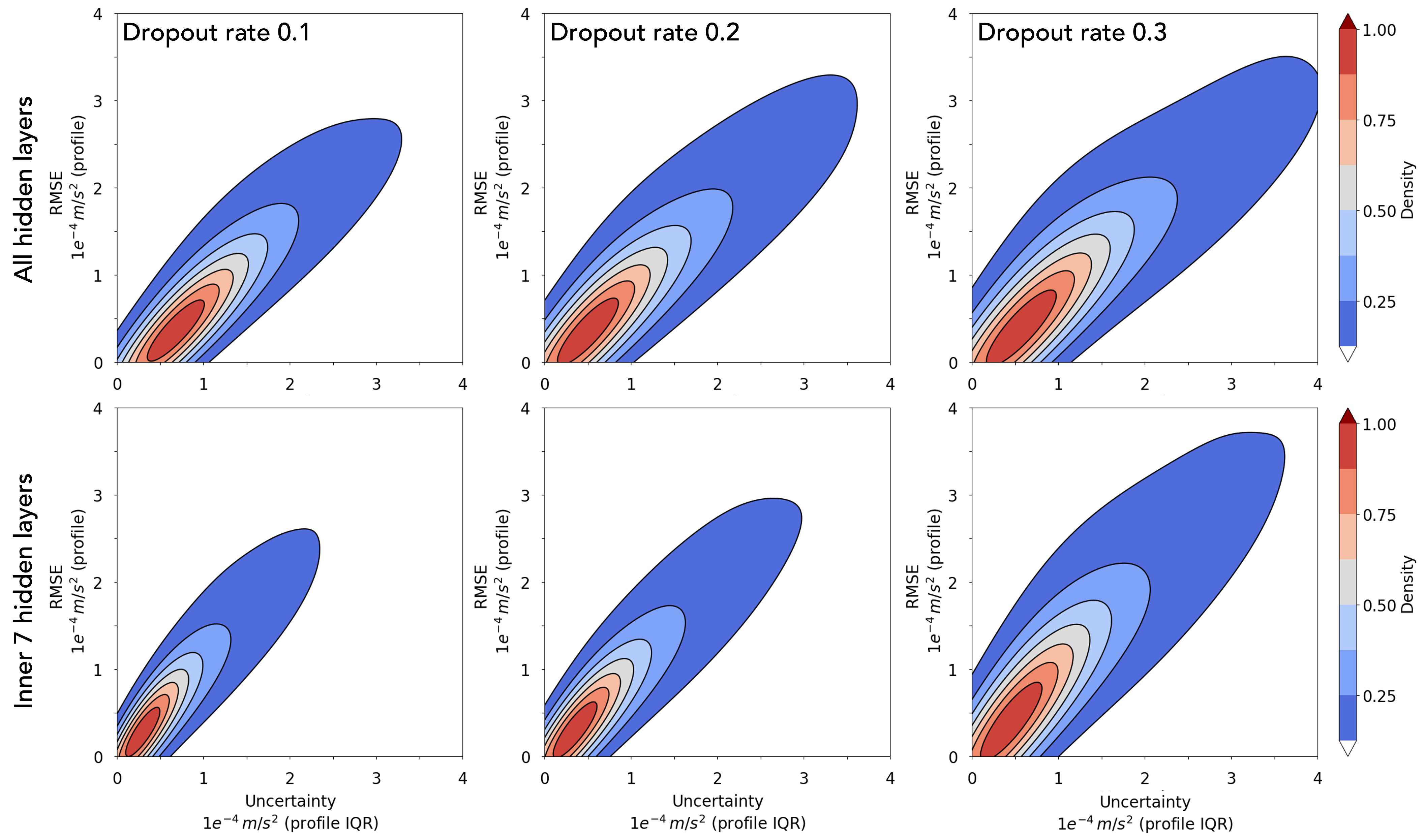
In addition to the hyperparameters of the deterministic NNs, designing an architecture for UQ often demands additional hyperparameter optimization. For instance, for the DNN, decisions need to be made regarding the number of neurons to drop out (dropout rate). While less common, one can also choose whether to apply dropout to all hidden layers or only selected ones. Variations in the dropout rate and the layers to which dropout is applied can influence the final configuration and performance of the DNN. Figure 13 illustrates these effects. As we increase the number of dropped neurons (whether through a higher dropout rate or by subjecting more layers to dropout), the uncertainty in the DNN predictions tends to rise. Yet, there is a persistent pattern in the relationship between spread (IQR) and RMSE across the various plots in Figure 13. Specifically, as spread increases, RMSE concurrently grows, consistent with the insights highlighted in Figure 9.
In the case of BNN or VAE, even though there is no dropout rate, there are distinct tuning opportunities available. For instance, with the VAE, one might consider applying dropout to the NN emulator. Moreover, given that the loss function in VAE comprises three components, decisions can be made regarding which component to penalize more heavily, allowing for nuanced adjustments to its performance.
Appendix C The UQ metrics
Each point in the spread-skill plot corresponds to one specific bin of ensemble spread (), which is defined as the average standard deviation of the ensemble members. We first separate the spread using a pre-selected number of bins (a subjective choice of 15 is used here). Then for the bin:
| (6) |
is the observed value for the example, is the mean prediction for the example, is the prediction for the example, is the total number of examples in the bin, and is the ensemble size. Following Haynes \BOthers. (\APACyear2023), we summarize the quality of the spread-skill plot by two measures: spread-skill reliability (SSREL) and overall spread-skill ratio (SSRAT). SSREL is the bin-weighted mean distance from the 1-to-1 line:
| (7) |
where is the total number of examples, is the total number of bins, and other variables are as in Equation 6. SSREL varies from , and the ideal value is 0. On the other hand, SSRAT is averaged over the whole dataset:
| (8) |
SSRAT also varies from , and the ideal value is 1. SSRAT 1 indicates the model is under-confident on average, while SSRAT 1 indicates that the model is overconfident on average.
In Equation (6), each level of a GWD profile is considered as an individual sample. As discussed earlier, while these samples help assess the model’s overall performance, our main interest is often the uncertainty of individual GWD profiles. Such uncertainty informs the trustworthiness of the model’s prediction for that specific profile. Accordingly, for each profile, we can compute:
| (9) |
where is the number of vertical levels for each profile, and is its interquartile range: corresponds with the 25th percentile, and corresponds with the 75th percentile.
Open Research
The data for all the analyses in the main text are available at https://doi.org/10.5281/zenodo.10019987. The emulator code is available at https://github.com/yqsun91/WACCM-Emulation. All the raw WACCM output data are available on request from authors.
Acknowledgements.
We thank Andre Souza for insightful discussions. This work was supported by grants from the NSF OAC CSSI program (#2005123 , #2004512, #2004492, #2004572), and by the generosity of Eric and Wendy Schmidt by recommendation of the Schmidt Futures program to PH, MJA, EG, and AS. PH is also supported by the Office of Naval Research (ONR) Young Investigator Award N00014-20-1-2722. SL is supported by the Office of Science, U.S. Department of Energy Biological and Environmental Research as part of the Regional and Global Climate Model Analysis program area. Computational resources were provided by NSF XSEDE (allocation ATM170020) and NCAR’s CISL (allocation URIC0009).References
- Abdar \BOthers. (\APACyear2021) \APACinsertmetastarABDAR2021243{APACrefauthors}Abdar, M., Pourpanah, F., Hussain, S., Rezazadegan, D., Liu, L., Ghavamzadeh, M.\BDBLNahavandi, S. \APACrefYearMonthDay2021. \BBOQ\APACrefatitleA review of uncertainty quantification in deep learning: Techniques, applications and challenges A review of uncertainty quantification in deep learning: Techniques, applications and challenges.\BBCQ \APACjournalVolNumPagesInformation Fusion76243-297. {APACrefURL} https://www.sciencedirect.com/science/article/pii/S1566253521001081 {APACrefDOI} https://doi.org/10.1016/j.inffus.2021.05.008 \PrintBackRefs\CurrentBib
- Achatz (\APACyear2022) \APACinsertmetastarAchatz2022{APACrefauthors}Achatz, U. \APACrefYearMonthDay2022. \BBOQ\APACrefatitleGravity Waves and Their Impact on the Atmospheric Flow Gravity waves and their impact on the atmospheric flow.\BBCQ \BIn \APACrefbtitleAtmospheric Dynamics Atmospheric dynamics (\BPGS 407–505). \APACaddressPublisherBerlin, HeidelbergSpringer Berlin Heidelberg. {APACrefURL} https://doi.org/10.1007/978-3-662-63941-2_10 {APACrefDOI} 10.1007/978-3-662-63941-2_10 \PrintBackRefs\CurrentBib
- Alexander \BOthers. (\APACyear2010) \APACinsertmetastarAlexander2010QJRMS{APACrefauthors}Alexander, M\BPBIJ., Geller, M., McLandress, C., Polavarapu, S., Preusse, P., Sassi, F.\BDBLWatanabe, S. \APACrefYearMonthDay2010. \BBOQ\APACrefatitleRecent developments in gravity-wave effects in climatemodels and the global distribution of gravity-wavemomentum flux from observations and models Recent developments in gravity-wave effects in climatemodels and the global distribution of gravity-wavemomentum flux from observations and models.\BBCQ \APACjournalVolNumPagesQuarterly Journal of the Royal Meteorological Society136. {APACrefDOI} 10.1002/qj.637 \PrintBackRefs\CurrentBib
- Amiramjadi \BOthers. (\APACyear2022) \APACinsertmetastarAmiramjadi2022{APACrefauthors}Amiramjadi, M., Plougonven, R., Mohebalhojeh, A\BPBIR.\BCBL \BBA Mirzaei, M. \APACrefYearMonthDay2022. \BBOQ\APACrefatitleUsing machine learning to estimate non-orographic gravity wave characteristics at source levels Using machine learning to estimate non-orographic gravity wave characteristics at source levels.\BBCQ \APACjournalVolNumPagesJournal of the Atmospheric Sciences. {APACrefDOI} 10.1175/JAS-D-22-0021.1 \PrintBackRefs\CurrentBib
- Ando \BBA Huang (\APACyear2017) \APACinsertmetastarando2017deep{APACrefauthors}Ando, S.\BCBT \BBA Huang, C\BPBIY. \APACrefYearMonthDay2017. \BBOQ\APACrefatitleDeep over-sampling framework for classifying imbalanced data Deep over-sampling framework for classifying imbalanced data.\BBCQ \BIn \APACrefbtitleMachine Learning and Knowledge Discovery in Databases: European Conference, ECML PKDD 2017, Skopje, Macedonia, September 18–22, 2017, Proceedings, Part I 10 Machine learning and knowledge discovery in databases: European conference, ecml pkdd 2017, skopje, macedonia, september 18–22, 2017, proceedings, part i 10 (\BPGS 770–785). \PrintBackRefs\CurrentBib
- Bacmeister \BOthers. (\APACyear1994) \APACinsertmetastarBacmeister1994{APACrefauthors}Bacmeister, J\BPBIT., Newman, P\BPBIA., Gary, B\BPBIL.\BCBL \BBA Chan, K\BPBIR. \APACrefYearMonthDay1994. \BBOQ\APACrefatitleAn algorithm for forecasting mountain wave-related turbulence in the stratosphere An algorithm for forecasting mountain wave-related turbulence in the stratosphere.\BBCQ \APACjournalVolNumPagesWeather and Forecasting9. {APACrefDOI} 10.1175/1520-0434(1994)009¡0241:AAFFMW¿2.0.CO;2 \PrintBackRefs\CurrentBib
- Balaji (\APACyear2021) \APACinsertmetastarbalaji2021climbing{APACrefauthors}Balaji, V. \APACrefYearMonthDay2021. \BBOQ\APACrefatitleClimbing down Charney’s ladder: machine learning and the post-Dennard era of computational climate science Climbing down charney’s ladder: machine learning and the post-dennard era of computational climate science.\BBCQ \APACjournalVolNumPagesPhilosophical Transactions of the Royal Society A379219420200085. \PrintBackRefs\CurrentBib
- Baldi \BOthers. (\APACyear2014) \APACinsertmetastarbaldi2014searching{APACrefauthors}Baldi, P., Sadowski, P.\BCBL \BBA Whiteson, D. \APACrefYearMonthDay2014. \BBOQ\APACrefatitleSearching for exotic particles in high-energy physics with deep learning Searching for exotic particles in high-energy physics with deep learning.\BBCQ \APACjournalVolNumPagesNature communications514308. \PrintBackRefs\CurrentBib
- Ballnus \BOthers. (\APACyear2017) \APACinsertmetastarballnus2017comprehensive{APACrefauthors}Ballnus, B., Hug, S., Hatz, K., Görlitz, L., Hasenauer, J.\BCBL \BBA Theis, F\BPBIJ. \APACrefYearMonthDay2017. \BBOQ\APACrefatitleComprehensive benchmarking of Markov chain Monte Carlo methods for dynamical systems Comprehensive benchmarking of markov chain monte carlo methods for dynamical systems.\BBCQ \APACjournalVolNumPagesBMC Systems Biology1111–18. \PrintBackRefs\CurrentBib
- Barnes \BOthers. (\APACyear2023) \APACinsertmetastarbarnes2023sinh{APACrefauthors}Barnes, E\BPBIA., Barnes, R\BPBIJ.\BCBL \BBA DeMaria, M. \APACrefYearMonthDay2023. \BBOQ\APACrefatitleSinh-arcsinh-normal distributions to add uncertainty to neural network regression tasks: Applications to tropical cyclone intensity forecasts Sinh-arcsinh-normal distributions to add uncertainty to neural network regression tasks: Applications to tropical cyclone intensity forecasts.\BBCQ \APACjournalVolNumPagesEnvironmental Data Science2e15. \PrintBackRefs\CurrentBib
- Beck \BOthers. (\APACyear2019) \APACinsertmetastarbeck2019deep{APACrefauthors}Beck, A., Flad, D.\BCBL \BBA Munz, C\BHBID. \APACrefYearMonthDay2019. \BBOQ\APACrefatitleDeep neural networks for data-driven LES closure models Deep neural networks for data-driven LES closure models.\BBCQ \APACjournalVolNumPagesJournal of Computational Physics398108910. \PrintBackRefs\CurrentBib
- Beljaars \BOthers. (\APACyear2004) \APACinsertmetastarBeljaars2004{APACrefauthors}Beljaars, A\BPBIC., Brown, A\BPBIR.\BCBL \BBA Wood, N. \APACrefYearMonthDay2004. \BBOQ\APACrefatitleA new parametrization of turbulent orographic form drag A new parametrization of turbulent orographic form drag.\BBCQ \APACjournalVolNumPagesQuarterly Journal of the Royal Meteorological Society130. {APACrefDOI} 10.1256/qj.03.73 \PrintBackRefs\CurrentBib
- Belochitski \BBA Krasnopolsky (\APACyear2021) \APACinsertmetastarbelochitskiKrasnopolsky2021{APACrefauthors}Belochitski, A.\BCBT \BBA Krasnopolsky, V. \APACrefYearMonthDay2021. \BBOQ\APACrefatitleRobustness of neural network emulations of radiative transfer parameterizations in a state-of-the-art general circulation model Robustness of neural network emulations of radiative transfer parameterizations in a state-of-the-art general circulation model.\BBCQ \APACjournalVolNumPagesGeoscientific Model Development14127425–7437. {APACrefURL} https://gmd.copernicus.org/articles/14/7425/2021/ {APACrefDOI} 10.5194/gmd-14-7425-2021 \PrintBackRefs\CurrentBib
- Beucler \BOthers. (\APACyear2021) \APACinsertmetastarBeuclerPritchard2021cloud{APACrefauthors}Beucler, T., Ebert-Uphoff, I., Rasp, S., Pritchard, M.\BCBL \BBA Gentine, P. \APACrefYearMonthDay202105. \APACrefbtitleMachine Learning for Clouds and Climate (Invited Chapter for the AGU Geophysical Monograph Series ”Clouds and Climate”). Machine learning for clouds and climate (invited chapter for the agu geophysical monograph series ”clouds and climate”). {APACrefDOI} 10.1002/essoar.10506925.1 \PrintBackRefs\CurrentBib
- Blundell \BOthers. (\APACyear2015) \APACinsertmetastarblundell2015weight{APACrefauthors}Blundell, C., Cornebise, J., Kavukcuoglu, K.\BCBL \BBA Wierstra, D. \APACrefYearMonthDay2015. \APACrefbtitleWeight Uncertainty in Neural Networks. Weight uncertainty in neural networks. \PrintBackRefs\CurrentBib
- Bolton \BBA Zanna (\APACyear2019) \APACinsertmetastarbolton2019applications{APACrefauthors}Bolton, T.\BCBT \BBA Zanna, L. \APACrefYearMonthDay2019. \BBOQ\APACrefatitleApplications of deep learning to ocean data inference and subgrid parameterization Applications of deep learning to ocean data inference and subgrid parameterization.\BBCQ \APACjournalVolNumPagesJournal of Advances in Modeling Earth Systems111376–399. \PrintBackRefs\CurrentBib
- Brenowitz \BOthers. (\APACyear2020) \APACinsertmetastarBrenowitz2020instability{APACrefauthors}Brenowitz, N\BPBID., Beucler, T., Pritchard, M.\BCBL \BBA Bretherton, C\BPBIS. \APACrefYearMonthDay2020. \BBOQ\APACrefatitleInterpreting and Stabilizing Machine-Learning Parametrizations of Convection Interpreting and stabilizing machine-learning parametrizations of convection.\BBCQ \APACjournalVolNumPagesJournal of the Atmospheric Sciences77124357 - 4375. {APACrefURL} https://journals.ametsoc.org/view/journals/atsc/77/12/jas-d-20-0082.1.xml {APACrefDOI} https://doi.org/10.1175/JAS-D-20-0082.1 \PrintBackRefs\CurrentBib
- Brenowitz \BBA Bretherton (\APACyear2019) \APACinsertmetastarbrenowitzBretherton2019{APACrefauthors}Brenowitz, N\BPBID.\BCBT \BBA Bretherton, C\BPBIS. \APACrefYearMonthDay2019. \BBOQ\APACrefatitleSpatially Extended Tests of a Neural Network Parametrization Trained by Coarse-Graining Spatially extended tests of a neural network parametrization trained by coarse-graining.\BBCQ \APACjournalVolNumPagesJournal of Advances in Modeling Earth Systems1182728-2744. {APACrefURL} https://agupubs.onlinelibrary.wiley.com/doi/abs/10.1029/2019MS001711 {APACrefDOI} https://doi.org/10.1029/2019MS001711 \PrintBackRefs\CurrentBib
- Buda \BOthers. (\APACyear2018) \APACinsertmetastarBUDA2018249{APACrefauthors}Buda, M., Maki, A.\BCBL \BBA Mazurowski, M\BPBIA. \APACrefYearMonthDay2018. \BBOQ\APACrefatitleA systematic study of the class imbalance problem in convolutional neural networks A systematic study of the class imbalance problem in convolutional neural networks.\BBCQ \APACjournalVolNumPagesNeural Networks106249-259. {APACrefURL} https://www.sciencedirect.com/science/article/pii/S0893608018302107 {APACrefDOI} https://doi.org/10.1016/j.neunet.2018.07.011 \PrintBackRefs\CurrentBib
- Bölöni \BOthers. (\APACyear2021) \APACinsertmetastarBoloni2021{APACrefauthors}Bölöni, G., Kim, Y\BPBIH., Borchert, S.\BCBL \BBA Achatz, U. \APACrefYearMonthDay2021. \BBOQ\APACrefatitleToward transient subgrid-scale gravity wave representation in atmospheric models. Part I: Propagation model including nondissipative wave mean-flow interactions Toward transient subgrid-scale gravity wave representation in atmospheric models. part i: Propagation model including nondissipative wave mean-flow interactions.\BBCQ \APACjournalVolNumPagesJournal of the Atmospheric Sciences78. {APACrefDOI} 10.1175/JAS-D-20-0065.1 \PrintBackRefs\CurrentBib
- Chantry \BOthers. (\APACyear2021) \APACinsertmetastarchantry2021{APACrefauthors}Chantry, M., Hatfield, S., Dueben, P., Polichtchouk, I.\BCBL \BBA Palmer, T. \APACrefYearMonthDay2021. \BBOQ\APACrefatitleMachine Learning Emulation of Gravity Wave Drag in Numerical Weather Forecasting Machine learning emulation of gravity wave drag in numerical weather forecasting.\BBCQ \APACjournalVolNumPagesJournal of Advances in Modeling Earth Systems137e2021MS002477. {APACrefURL} https://agupubs.onlinelibrary.wiley.com/doi/abs/10.1029/2021MS002477 \APACrefnotee2021MS002477 2021MS002477 {APACrefDOI} https://doi.org/10.1029/2021MS002477 \PrintBackRefs\CurrentBib
- Chattopadhyay, Nabizadeh\BCBL \BBA Hassanzadeh (\APACyear2020) \APACinsertmetastarchattopadhyay2020analog{APACrefauthors}Chattopadhyay, A., Nabizadeh, E.\BCBL \BBA Hassanzadeh, P. \APACrefYearMonthDay2020. \BBOQ\APACrefatitleAnalog forecasting of extreme-causing weather patterns using deep learning Analog forecasting of extreme-causing weather patterns using deep learning.\BBCQ \APACjournalVolNumPagesJournal of Advances in Modeling Earth Systems122e2019MS001958. \PrintBackRefs\CurrentBib
- Chattopadhyay, Subel\BCBL \BBA Hassanzadeh (\APACyear2020) \APACinsertmetastarchattopadhyay2020data{APACrefauthors}Chattopadhyay, A., Subel, A.\BCBL \BBA Hassanzadeh, P. \APACrefYearMonthDay2020. \BBOQ\APACrefatitleData-driven super-parameterization using deep learning: Experimentation with multiscale Lorenz 96 systems and transfer learning Data-driven super-parameterization using deep learning: Experimentation with multiscale Lorenz 96 systems and transfer learning.\BBCQ \APACjournalVolNumPagesJournal of Advances in Modeling Earth Systems1211e2020MS002084. \PrintBackRefs\CurrentBib
- Chawla \BOthers. (\APACyear2004) \APACinsertmetastarChawla_etal_2004{APACrefauthors}Chawla, N\BPBIV., Japkowicz, N.\BCBL \BBA Kotcz, A. \APACrefYearMonthDay2004jun. \BBOQ\APACrefatitleEditorial: Special Issue on Learning from Imbalanced Data Sets Editorial: Special issue on learning from imbalanced data sets.\BBCQ \APACjournalVolNumPagesSIGKDD Explor. Newsl.611–6. {APACrefURL} https://doi.org/10.1145/1007730.1007733 {APACrefDOI} 10.1145/1007730.1007733 \PrintBackRefs\CurrentBib
- Chen \BBA Majda (\APACyear2019) \APACinsertmetastarchen2019new{APACrefauthors}Chen, N.\BCBT \BBA Majda, A\BPBIJ. \APACrefYearMonthDay2019. \BBOQ\APACrefatitleA new efficient parameter estimation algorithm for high-dimensional complex nonlinear turbulent dynamical systems with partial observations A new efficient parameter estimation algorithm for high-dimensional complex nonlinear turbulent dynamical systems with partial observations.\BBCQ \APACjournalVolNumPagesJournal of Computational Physics397108836. \PrintBackRefs\CurrentBib
- Clare \BOthers. (\APACyear2022) \APACinsertmetastarclare2022explainable{APACrefauthors}Clare, M\BPBIC., Sonnewald, M., Lguensat, R., Deshayes, J.\BCBL \BBA Balaji, V. \APACrefYearMonthDay2022. \BBOQ\APACrefatitleExplainable Artificial Intelligence for Bayesian Neural Networks: Towards trustworthy predictions of ocean dynamics Explainable artificial intelligence for bayesian neural networks: Towards trustworthy predictions of ocean dynamics.\BBCQ \APACjournalVolNumPagesarXiv preprint arXiv:2205.00202. \PrintBackRefs\CurrentBib
- Delle Monache \BOthers. (\APACyear2013) \APACinsertmetastardelle2013probabilistic{APACrefauthors}Delle Monache, L., Eckel, F\BPBIA., Rife, D\BPBIL., Nagarajan, B.\BCBL \BBA Searight, K. \APACrefYearMonthDay2013. \BBOQ\APACrefatitleProbabilistic weather prediction with an analog ensemble Probabilistic weather prediction with an analog ensemble.\BBCQ \APACjournalVolNumPagesMonthly Weather Review141103498–3516. \PrintBackRefs\CurrentBib
- Dong \BOthers. (\APACyear2023) \APACinsertmetastarDongetal2023{APACrefauthors}Dong, W., Fritts, D\BPBIC., Liu, A\BPBIZ., Lund, T\BPBIS., Liu, H\BHBIL.\BCBL \BBA Snively, J. \APACrefYearMonthDay2023. \BBOQ\APACrefatitleAccelerating Atmospheric Gravity Wave Simulations Using Machine Learning: Kelvin-Helmholtz Instability and Mountain Wave Sources Driving Gravity Wave Breaking and Secondary Gravity Wave Generation Accelerating atmospheric gravity wave simulations using machine learning: Kelvin-helmholtz instability and mountain wave sources driving gravity wave breaking and secondary gravity wave generation.\BBCQ \APACjournalVolNumPagesGeophysical Research Letters5015e2023GL104668. {APACrefURL} https://agupubs.onlinelibrary.wiley.com/doi/abs/10.1029/2023GL104668 \APACrefnotee2023GL104668 2023GL104668 {APACrefDOI} https://doi.org/10.1029/2023GL104668 \PrintBackRefs\CurrentBib
- Espinosa \BOthers. (\APACyear2022) \APACinsertmetastarEspinosa2022{APACrefauthors}Espinosa, Z\BPBII., Sheshadri, A., Cain, G\BPBIR., Gerber, E\BPBIP.\BCBL \BBA DallaSanta, K\BPBIJ. \APACrefYearMonthDay2022. \BBOQ\APACrefatitleMachine learning gravity wave parameterization generalizes to capture the QBO and response to increased CO2 Machine learning gravity wave parameterization generalizes to capture the qbo and response to increased co2.\BBCQ \APACjournalVolNumPagesGeophysical Research Letters498e2022GL098174. \PrintBackRefs\CurrentBib
- Finkel \BOthers. (\APACyear2023) \APACinsertmetastarFinkeletal2023{APACrefauthors}Finkel, J., Gerber, E\BPBIP., Abbot, D\BPBIS.\BCBL \BBA Weare, J. \APACrefYearMonthDay2023. \BBOQ\APACrefatitleRevealing the Statistics of Extreme Events Hidden in Short Weather Forecast Data Revealing the statistics of extreme events hidden in short weather forecast data.\BBCQ \APACjournalVolNumPagesAGU Advances42e2023AV000881. {APACrefURL} https://agupubs.onlinelibrary.wiley.com/doi/abs/10.1029/2023AV000881 \APACrefnotee2023AV000881 2023AV000881 {APACrefDOI} https://doi.org/10.1029/2023AV000881 \PrintBackRefs\CurrentBib
- Foster \BOthers. (\APACyear2021) \APACinsertmetastarFoster2021{APACrefauthors}Foster, D., Gagne, D\BPBIJ.\BCBL \BBA Whitt, D\BPBIB. \APACrefYearMonthDay202112. \BBOQ\APACrefatitleProbabilistic Machine Learning Estimation of Ocean Mixed Layer Depth From Dense Satellite and Sparse In Situ Observations Probabilistic machine learning estimation of ocean mixed layer depth from dense satellite and sparse in situ observations.\BBCQ \APACjournalVolNumPagesJournal of Advances in Modeling Earth Systems13. {APACrefDOI} 10.1029/2021MS002474 \PrintBackRefs\CurrentBib
- Frezat \BOthers. (\APACyear2022) \APACinsertmetastarfrezat2022posteriori{APACrefauthors}Frezat, H., Sommer, J\BPBIL., Fablet, R., Balarac, G.\BCBL \BBA Lguensat, R. \APACrefYearMonthDay2022. \BBOQ\APACrefatitleA posteriori learning for quasi-geostrophic turbulence parametrization A posteriori learning for quasi-geostrophic turbulence parametrization.\BBCQ \APACjournalVolNumPagesarXiv preprint arXiv:2204.03911. {APACrefDOI} 10.1029/2022MS003124 \PrintBackRefs\CurrentBib
- Gagne \BOthers. (\APACyear2020) \APACinsertmetastargagne2020machine{APACrefauthors}Gagne, D\BPBIJ., Christensen, H\BPBIM., Subramanian, A\BPBIC.\BCBL \BBA Monahan, A\BPBIH. \APACrefYearMonthDay2020. \BBOQ\APACrefatitleMachine learning for stochastic parameterization: Generative adversarial networks in the Lorenz’96 model Machine learning for stochastic parameterization: Generative adversarial networks in the lorenz’96 model.\BBCQ \APACjournalVolNumPagesJournal of Advances in Modeling Earth Systems123e2019MS001896. \PrintBackRefs\CurrentBib
- Gal \BBA Ghahramani (\APACyear2016) \APACinsertmetastargal2016dropout{APACrefauthors}Gal, Y.\BCBT \BBA Ghahramani, Z. \APACrefYearMonthDay2016. \BBOQ\APACrefatitleDropout as a bayesian approximation: Representing model uncertainty in deep learning Dropout as a bayesian approximation: Representing model uncertainty in deep learning.\BBCQ \BIn \APACrefbtitleinternational conference on machine learning international conference on machine learning (\BPGS 1050–1059). \PrintBackRefs\CurrentBib
- Garcia \BOthers. (\APACyear2017) \APACinsertmetastarGarciaOGW-WACCM2017{APACrefauthors}Garcia, R\BPBIR., Smith, A\BPBIK., Kinnison, D\BPBIE., Álvaro de la Cámara\BCBL \BBA Murphy, D\BPBIJ. \APACrefYearMonthDay2017. \BBOQ\APACrefatitleModification of the Gravity Wave Parameterization in the Whole Atmosphere Community Climate Model: Motivation and Results Modification of the gravity wave parameterization in the whole atmosphere community climate model: Motivation and results.\BBCQ \APACjournalVolNumPagesJournal of the Atmospheric Sciences741275 - 291. {APACrefURL} https://journals.ametsoc.org/view/journals/atsc/74/1/jas-d-16-0104.1.xml {APACrefDOI} https://doi.org/10.1175/JAS-D-16-0104.1 \PrintBackRefs\CurrentBib
- Geller \BOthers. (\APACyear2013) \APACinsertmetastargeller2013comparison{APACrefauthors}Geller, M\BPBIA., Alexander, M\BPBIJ., Love, P\BPBIT., Bacmeister, J., Ern, M., Hertzog, A.\BDBLothers \APACrefYearMonthDay2013. \BBOQ\APACrefatitleA comparison between gravity wave momentum fluxes in observations and climate models A comparison between gravity wave momentum fluxes in observations and climate models.\BBCQ \APACjournalVolNumPagesJournal of Climate26176383–6405. \PrintBackRefs\CurrentBib
- Gettelman \BOthers. (\APACyear2021) \APACinsertmetastarGettelman2021{APACrefauthors}Gettelman, A., Gagne, D\BPBIJ., Chen, C\BPBIC., Christensen, M\BPBIW., Lebo, Z\BPBIJ., Morrison, H.\BCBL \BBA Gantos, G. \APACrefYearMonthDay2021. \BBOQ\APACrefatitleMachine Learning the Warm Rain Process Machine learning the warm rain process.\BBCQ \APACjournalVolNumPagesJournal of Advances in Modeling Earth Systems13. {APACrefDOI} 10.1029/2020MS002268 \PrintBackRefs\CurrentBib
- Gettelman \BOthers. (\APACyear2019) \APACinsertmetastarGettelman2019{APACrefauthors}Gettelman, A., Mills, M\BPBIJ., Kinnison, D\BPBIE., Garcia, R\BPBIR., Smith, A\BPBIK., Marsh, D\BPBIR.\BDBLRandel, W\BPBIJ. \APACrefYearMonthDay201912. \BBOQ\APACrefatitleThe Whole Atmosphere Community Climate Model Version 6 (WACCM6) The whole atmosphere community climate model version 6 (waccm6).\BBCQ \APACjournalVolNumPagesJournal of Geophysical Research: Atmospheres12412380-12403. {APACrefDOI} 10.1029/2019JD030943 \PrintBackRefs\CurrentBib
- Gordon \BBA Barnes (\APACyear2022) \APACinsertmetastarGordon2022{APACrefauthors}Gordon, E\BPBIM.\BCBT \BBA Barnes, E\BPBIA. \APACrefYearMonthDay20228. \BBOQ\APACrefatitleIncorporating Uncertainty Into a Regression Neural Network Enables Identification of Decadal State-Dependent Predictability in CESM2 Incorporating uncertainty into a regression neural network enables identification of decadal state-dependent predictability in cesm2.\BBCQ \APACjournalVolNumPagesGeophysical Research Letters49. {APACrefDOI} 10.1029/2022GL098635 \PrintBackRefs\CurrentBib
- Guan \BOthers. (\APACyear2022) \APACinsertmetastarguan2022stable{APACrefauthors}Guan, Y., Chattopadhyay, A., Subel, A.\BCBL \BBA Hassanzadeh, P. \APACrefYearMonthDay2022. \BBOQ\APACrefatitleStable a posteriori LES of 2D turbulence using convolutional neural networks: Backscattering analysis and generalization to higher Re via transfer learning Stable a posteriori LES of 2D turbulence using convolutional neural networks: Backscattering analysis and generalization to higher Re via transfer learning.\BBCQ \APACjournalVolNumPagesJournal of Computational Physics458111090. \PrintBackRefs\CurrentBib
- Guan \BOthers. (\APACyear2023) \APACinsertmetastarguan2022learning{APACrefauthors}Guan, Y., Subel, A., Chattopadhyay, A.\BCBL \BBA Hassanzadeh, P. \APACrefYearMonthDay2023. \BBOQ\APACrefatitleLearning physics-constrained subgrid-scale closures in the small-data regime for stable and accurate LES Learning physics-constrained subgrid-scale closures in the small-data regime for stable and accurate les.\BBCQ \APACjournalVolNumPagesPhysica D: Nonlinear Phenomena443133568. {APACrefDOI} https://doi.org/10.1016/j.physd.2022.133568 \PrintBackRefs\CurrentBib
- Guillaumin \BBA Zanna (\APACyear2021) \APACinsertmetastarguillaumin2021stochastic{APACrefauthors}Guillaumin, A\BPBIP.\BCBT \BBA Zanna, L. \APACrefYearMonthDay2021. \BBOQ\APACrefatitleStochastic-deep learning parameterization of ocean momentum forcing Stochastic-deep learning parameterization of ocean momentum forcing.\BBCQ \APACjournalVolNumPagesJournal of Advances in Modeling Earth Systems139e2021MS002534. \PrintBackRefs\CurrentBib
- Hardiman \BOthers. (\APACyear2023) \APACinsertmetastarhardiman2023machine{APACrefauthors}Hardiman, S\BPBIC., Scaife, A\BPBIA., Niekerk, A\BPBIv., Prudden, R., Owen, A., Adams, S\BPBIV.\BDBLMadge, S. \APACrefYearMonthDay2023. \BBOQ\APACrefatitleMachine learning for non-orographic gravity waves in a climate model Machine learning for non-orographic gravity waves in a climate model.\BBCQ \APACjournalVolNumPagesArtificial Intelligence for the Earth Systems. \PrintBackRefs\CurrentBib
- Haynes \BOthers. (\APACyear2023) \APACinsertmetastarhaynes2023creating{APACrefauthors}Haynes, K., Lagerquist, R., McGraw, M., Musgrave, K.\BCBL \BBA Ebert-Uphoff, I. \APACrefYearMonthDay2023. \BBOQ\APACrefatitleCreating and evaluating uncertainty estimates with neural networks for environmental-science applications Creating and evaluating uncertainty estimates with neural networks for environmental-science applications.\BBCQ \APACjournalVolNumPagesArtificial Intelligence for the Earth Systems1–58. \PrintBackRefs\CurrentBib
- Hertzog \BOthers. (\APACyear2012) \APACinsertmetastarhertzog2012intermittency{APACrefauthors}Hertzog, A., Alexander, M\BPBIJ.\BCBL \BBA Plougonven, R. \APACrefYearMonthDay2012. \BBOQ\APACrefatitleOn the intermittency of gravity wave momentum flux in the stratosphere On the intermittency of gravity wave momentum flux in the stratosphere.\BBCQ \APACjournalVolNumPagesJournal of the Atmospheric Sciences69113433–3448. \PrintBackRefs\CurrentBib
- Hourdin \BOthers. (\APACyear2017) \APACinsertmetastarhourdin2017art{APACrefauthors}Hourdin, F., Mauritsen, T., Gettelman, A., Golaz, J\BHBIC., Balaji, V., Duan, Q.\BDBLothers \APACrefYearMonthDay2017. \BBOQ\APACrefatitleThe art and science of climate model tuning The art and science of climate model tuning.\BBCQ \APACjournalVolNumPagesBulletin of the American Meteorological Society983589–602. \PrintBackRefs\CurrentBib
- Huang \BOthers. (\APACyear2016) \APACinsertmetastarhuang2016learning{APACrefauthors}Huang, C., Li, Y., Loy, C\BPBIC.\BCBL \BBA Tang, X. \APACrefYearMonthDay2016. \BBOQ\APACrefatitleLearning deep representation for imbalanced classification Learning deep representation for imbalanced classification.\BBCQ \BIn \APACrefbtitleProceedings of the IEEE conference on computer vision and pattern recognition Proceedings of the ieee conference on computer vision and pattern recognition (\BPGS 5375–5384). \PrintBackRefs\CurrentBib
- Iglesias-Suarez \BOthers. (\APACyear2023) \APACinsertmetastariglesiassuarez2023causallyinformed{APACrefauthors}Iglesias-Suarez, F., Gentine, P., Solino-Fernandez, B., Beucler, T., Pritchard, M., Runge, J.\BCBL \BBA Eyring, V. \APACrefYearMonthDay2023. \APACrefbtitleCausally-informed deep learning to improve climate models and projections. Causally-informed deep learning to improve climate models and projections. \PrintBackRefs\CurrentBib
- Japkowicz \BBA Stephen (\APACyear2002) \APACinsertmetastarJapkowicz2002{APACrefauthors}Japkowicz, N.\BCBT \BBA Stephen, S. \APACrefYearMonthDay2002. \BBOQ\APACrefatitleThe class imbalance problem: A systematic study The class imbalance problem: A systematic study.\BBCQ \APACjournalVolNumPagesIntelligent Data Analysis6429-449. {APACrefURL} https://doi.org/10.3233/IDA-2002-6504 \APACrefnote5 {APACrefDOI} 10.3233/IDA-2002-6504 \PrintBackRefs\CurrentBib
- Johnson \BBA Khoshgoftaar (\APACyear2019) \APACinsertmetastarJohnson2019{APACrefauthors}Johnson, J\BPBIM.\BCBT \BBA Khoshgoftaar, T\BPBIM. \APACrefYearMonthDay2019Mar19. \BBOQ\APACrefatitleSurvey on deep learning with class imbalance Survey on deep learning with class imbalance.\BBCQ \APACjournalVolNumPagesJournal of Big Data6127. {APACrefURL} https://doi.org/10.1186/s40537-019-0192-5 {APACrefDOI} 10.1186/s40537-019-0192-5 \PrintBackRefs\CurrentBib
- Kim \BOthers. (\APACyear2021) \APACinsertmetastarKim2021JAS{APACrefauthors}Kim, Y., Bölöni, G., Borchert, S., Chun, H\BPBIY.\BCBL \BBA Achatz, U. \APACrefYearMonthDay2021. \BBOQ\APACrefatitleToward transient subgrid-scale gravity wave representation in atmospheric models. Part II: Wave intermittency simulated with convective sources Toward transient subgrid-scale gravity wave representation in atmospheric models. part ii: Wave intermittency simulated with convective sources.\BBCQ \APACjournalVolNumPagesJournal of the Atmospheric Sciences78. {APACrefDOI} 10.1175/JAS-D-20-0066.1 \PrintBackRefs\CurrentBib
- Kim \BOthers. (\APACyear2003) \APACinsertmetastarKimetal2003{APACrefauthors}Kim, Y., Eckermann, S\BPBID.\BCBL \BBA Chun, H. \APACrefYearMonthDay2003. \BBOQ\APACrefatitleAn overview of the past, present and future of gravity‐wave drag parametrization for numerical climate and weather prediction models An overview of the past, present and future of gravity‐wave drag parametrization for numerical climate and weather prediction models.\BBCQ \APACjournalVolNumPagesAtmosphere-Ocean4165-98. {APACrefURL} https://doi.org/10.3137/ao.410105 {APACrefDOI} 10.3137/ao.410105 \PrintBackRefs\CurrentBib
- Kingma \BBA Welling (\APACyear2014) \APACinsertmetastarKingma2014{APACrefauthors}Kingma, D\BPBIP.\BCBT \BBA Welling, M. \APACrefYearMonthDay2014. \BBOQ\APACrefatitleAuto-encoding variational bayes Auto-encoding variational bayes.\BBCQ \APACjournalVolNumPages2nd International Conference on Learning Representations, ICLR 2014 - Conference Track Proceedings. \PrintBackRefs\CurrentBib
- Köhler \BOthers. (\APACyear2023) \APACinsertmetastarkohler2023comparing{APACrefauthors}Köhler, L., Green, B.\BCBL \BBA Stephan, C\BPBIC. \APACrefYearMonthDay2023. \BBOQ\APACrefatitleComparing Loon Superpressure Balloon Observations of Gravity Waves in the Tropics With Global Storm-Resolving Models Comparing loon superpressure balloon observations of gravity waves in the tropics with global storm-resolving models.\BBCQ \APACjournalVolNumPagesJournal of Geophysical Research: Atmospheres12815e2023JD038549. \PrintBackRefs\CurrentBib
- Krasnopolsky \BOthers. (\APACyear2005) \APACinsertmetastarKrasnopolsky2005{APACrefauthors}Krasnopolsky, V\BPBIM., Fox-Rabinovitz, M\BPBIS.\BCBL \BBA Chalikov, D\BPBIV. \APACrefYearMonthDay2005. \BBOQ\APACrefatitleNew Approach to Calculation of Atmospheric Model Physics: Accurate and Fast Neural Network Emulation of Longwave Radiation in a Climate Model New approach to calculation of atmospheric model physics: Accurate and fast neural network emulation of longwave radiation in a climate model.\BBCQ \APACjournalVolNumPagesMonthly Weather Review13351370 - 1383. {APACrefURL} https://journals.ametsoc.org/view/journals/mwre/133/5/mwr2923.1.xml {APACrefDOI} https://doi.org/10.1175/MWR2923.1 \PrintBackRefs\CurrentBib
- Krueger \BOthers. (\APACyear2021) \APACinsertmetastarkrueger2021out{APACrefauthors}Krueger, D., Caballero, E., Jacobsen, J\BHBIH., Zhang, A., Binas, J., Zhang, D.\BDBLCourville, A. \APACrefYearMonthDay2021. \BBOQ\APACrefatitleOut-of-distribution generalization via risk extrapolation (rex) Out-of-distribution generalization via risk extrapolation (rex).\BBCQ \BIn \APACrefbtitleInternational Conference on Machine Learning International conference on machine learning (\BPGS 5815–5826). \PrintBackRefs\CurrentBib
- Kruse \BOthers. (\APACyear2022) \APACinsertmetastarKruse2022{APACrefauthors}Kruse, C\BPBIG., Alexander, M\BPBIJ., Hoffmann, L., Niekerk, A\BPBIV., Polichtchouk, I., Bacmeister, J\BPBIT.\BDBLStein, O. \APACrefYearMonthDay2022. \BBOQ\APACrefatitleObserved and Modeled Mountain Waves from the Surface to the Mesosphere near the Drake Passage Observed and modeled mountain waves from the surface to the mesosphere near the drake passage.\BBCQ \APACjournalVolNumPagesJournal of the Atmospheric Sciences79. {APACrefDOI} 10.1175/JAS-D-21-0252.1 \PrintBackRefs\CurrentBib
- Li \BOthers. (\APACyear2022) \APACinsertmetastarli2022uncertainty{APACrefauthors}Li, X., Dai, Y., Ge, Y., Liu, J., Shan, Y.\BCBL \BBA Duan, L\BHBIY. \APACrefYearMonthDay2022. \BBOQ\APACrefatitleUncertainty modeling for out-of-distribution generalization Uncertainty modeling for out-of-distribution generalization.\BBCQ \APACjournalVolNumPagesarXiv preprint arXiv:2202.03958. \PrintBackRefs\CurrentBib
- Ling \BBA Templeton (\APACyear2015) \APACinsertmetastarLingetal2015{APACrefauthors}Ling, J.\BCBT \BBA Templeton, J. \APACrefYearMonthDay201508. \BBOQ\APACrefatitleEvaluation of machine learning algorithms for prediction of regions of high Reynolds averaged Navier Stokes uncertainty Evaluation of machine learning algorithms for prediction of regions of high Reynolds averaged Navier Stokes uncertainty.\BBCQ \APACjournalVolNumPagesPhysics of Fluids278. {APACrefURL} https://doi.org/10.1063/1.4927765 \APACrefnote085103 {APACrefDOI} 10.1063/1.4927765 \PrintBackRefs\CurrentBib
- Liu \BOthers. (\APACyear2016) \APACinsertmetastarLiuDNNextreme2016{APACrefauthors}Liu, Y., Racah, E., Correa, J., Khosrowshahi, A., Lavers, D., Kunkel, K.\BDBLothers \APACrefYearMonthDay2016. \BBOQ\APACrefatitleApplication of deep convolutional neural networks for detecting extreme weather in climate datasets Application of deep convolutional neural networks for detecting extreme weather in climate datasets.\BBCQ \APACjournalVolNumPagesarXiv preprint arXiv:1605.01156. \PrintBackRefs\CurrentBib
- Lopez-Gomez \BOthers. (\APACyear2022) \APACinsertmetastarGomez2022HeatWave{APACrefauthors}Lopez-Gomez, I., McGovern, A., Agrawal, S.\BCBL \BBA Hickey, J. \APACrefYearMonthDay2022. \BBOQ\APACrefatitleGlobal Extreme Heat Forecasting Using Neural Weather Models Global extreme heat forecasting using neural weather models.\BBCQ \APACjournalVolNumPagesArtificial Intelligence for the Earth Systems1 - 41. {APACrefURL} https://journals.ametsoc.org/view/journals/aies/aop/AIES-D-22-0035.1/AIES-D-22-0035.1.xml {APACrefDOI} 10.1175/AIES-D-22-0035.1 \PrintBackRefs\CurrentBib
- Lu \BOthers. (\APACyear2021) \APACinsertmetastarlu2021learning{APACrefauthors}Lu, L., Jin, P., Pang, G., Zhang, Z.\BCBL \BBA Karniadakis, G\BPBIE. \APACrefYearMonthDay2021. \BBOQ\APACrefatitleLearning nonlinear operators via DeepONet based on the universal approximation theorem of operators Learning nonlinear operators via deeponet based on the universal approximation theorem of operators.\BBCQ \APACjournalVolNumPagesNature machine intelligence33218–229. \PrintBackRefs\CurrentBib
- Maalouf \BBA Siddiqi (\APACyear2014) \APACinsertmetastarmaalouf2014weighted{APACrefauthors}Maalouf, M.\BCBT \BBA Siddiqi, M. \APACrefYearMonthDay2014. \BBOQ\APACrefatitleWeighted logistic regression for large-scale imbalanced and rare events data Weighted logistic regression for large-scale imbalanced and rare events data.\BBCQ \APACjournalVolNumPagesKnowledge-Based Systems59142–148. \PrintBackRefs\CurrentBib
- Maalouf \BBA Trafalis (\APACyear2011) \APACinsertmetastarmaalouf2011robust{APACrefauthors}Maalouf, M.\BCBT \BBA Trafalis, T\BPBIB. \APACrefYearMonthDay2011. \BBOQ\APACrefatitleRobust weighted kernel logistic regression in imbalanced and rare events data Robust weighted kernel logistic regression in imbalanced and rare events data.\BBCQ \APACjournalVolNumPagesComputational Statistics & Data Analysis551168–183. \PrintBackRefs\CurrentBib
- Maddox \BOthers. (\APACyear2019) \APACinsertmetastarmaddox2019simple{APACrefauthors}Maddox, W\BPBIJ., Izmailov, P., Garipov, T., Vetrov, D\BPBIP.\BCBL \BBA Wilson, A\BPBIG. \APACrefYearMonthDay2019. \BBOQ\APACrefatitleA Simple Baseline for Bayesian Uncertainty in Deep Learning A simple baseline for bayesian uncertainty in deep learning.\BBCQ \APACjournalVolNumPagesAdvances in Neural Information Processing Systems32. \PrintBackRefs\CurrentBib
- Mamalakis \BOthers. (\APACyear2022) \APACinsertmetastarmamalakis2022investigating{APACrefauthors}Mamalakis, A., Barnes, E\BPBIA.\BCBL \BBA Ebert-Uphoff, I. \APACrefYearMonthDay2022. \BBOQ\APACrefatitleInvestigating the fidelity of explainable artificial intelligence methods for applications of convolutional neural networks in geoscience Investigating the fidelity of explainable artificial intelligence methods for applications of convolutional neural networks in geoscience.\BBCQ \APACjournalVolNumPagesArtificial Intelligence for the Earth Systems14e220012. \PrintBackRefs\CurrentBib
- Matsuoka \BOthers. (\APACyear2020) \APACinsertmetastarMatsuoka2020{APACrefauthors}Matsuoka, D., Watanabe, S., Sato, K., Kawazoe, S., Yu, W.\BCBL \BBA Easterbrook, S. \APACrefYearMonthDay2020. \BBOQ\APACrefatitleApplication of deep learning to estimate atmospheric gravity wave parameters in reanalysis data sets Application of deep learning to estimate atmospheric gravity wave parameters in reanalysis data sets.\BBCQ \APACjournalVolNumPagesGeophysical Research Letters4719e2020GL089436. \PrintBackRefs\CurrentBib
- Maulik \BOthers. (\APACyear2019) \APACinsertmetastarmaulik2019subgrid{APACrefauthors}Maulik, R., San, O., Rasheed, A.\BCBL \BBA Vedula, P. \APACrefYearMonthDay2019. \BBOQ\APACrefatitleSubgrid modelling for two-dimensional turbulence using neural networks Subgrid modelling for two-dimensional turbulence using neural networks.\BBCQ \APACjournalVolNumPagesJournal of Fluid Mechanics858122–144. \PrintBackRefs\CurrentBib
- McGovern \BOthers. (\APACyear2019) \APACinsertmetastarMcGovern2019{APACrefauthors}McGovern, A., Lagerquist, R., Gagne, D\BPBIJ., Jergensen, G\BPBIE., Elmore, K\BPBIL., Homeyer, C\BPBIR.\BCBL \BBA Smith, T. \APACrefYearMonthDay2019. \BBOQ\APACrefatitleMaking the black box more transparent: Understanding the physical implications of machine learning Making the black box more transparent: Understanding the physical implications of machine learning.\BBCQ \APACjournalVolNumPagesBulletin of the American Meteorological Society100. {APACrefDOI} 10.1175/BAMS-D-18-0195.1 \PrintBackRefs\CurrentBib
- Miller \BOthers. (\APACyear2021) \APACinsertmetastarmiller2021accuracy{APACrefauthors}Miller, J\BPBIP., Taori, R., Raghunathan, A., Sagawa, S., Koh, P\BPBIW., Shankar, V.\BDBLSchmidt, L. \APACrefYearMonthDay2021. \BBOQ\APACrefatitleAccuracy on the line: on the strong correlation between out-of-distribution and in-distribution generalization Accuracy on the line: on the strong correlation between out-of-distribution and in-distribution generalization.\BBCQ \BIn \APACrefbtitleInternational Conference on Machine Learning International conference on machine learning (\BPGS 7721–7735). \PrintBackRefs\CurrentBib
- Miloshevich \BOthers. (\APACyear2023) \APACinsertmetastarPhysRevFluids.8.040501{APACrefauthors}Miloshevich, G., Cozian, B., Abry, P., Borgnat, P.\BCBL \BBA Bouchet, F. \APACrefYearMonthDay2023Apr. \BBOQ\APACrefatitleProbabilistic forecasts of extreme heatwaves using convolutional neural networks in a regime of lack of data Probabilistic forecasts of extreme heatwaves using convolutional neural networks in a regime of lack of data.\BBCQ \APACjournalVolNumPagesPhys. Rev. Fluids8040501. {APACrefURL} https://link.aps.org/doi/10.1103/PhysRevFluids.8.040501 {APACrefDOI} 10.1103/PhysRevFluids.8.040501 \PrintBackRefs\CurrentBib
- Nagarajan \BOthers. (\APACyear2020) \APACinsertmetastarnagarajan2020understanding{APACrefauthors}Nagarajan, V., Andreassen, A.\BCBL \BBA Neyshabur, B. \APACrefYearMonthDay2020. \BBOQ\APACrefatitleUnderstanding the failure modes of out-of-distribution generalization Understanding the failure modes of out-of-distribution generalization.\BBCQ \APACjournalVolNumPagesarXiv preprint arXiv:2010.15775. \PrintBackRefs\CurrentBib
- O’Gorman \BBA Dwyer (\APACyear2018) \APACinsertmetastarGormanDwyer2018{APACrefauthors}O’Gorman, P\BPBIA.\BCBT \BBA Dwyer, J\BPBIG. \APACrefYearMonthDay2018. \BBOQ\APACrefatitleUsing Machine Learning to Parameterize Moist Convection: Potential for Modeling of Climate, Climate Change, and Extreme Events Using machine learning to parameterize moist convection: Potential for modeling of climate, climate change, and extreme events.\BBCQ \APACjournalVolNumPagesJournal of Advances in Modeling Earth Systems10102548-2563. {APACrefURL} https://agupubs.onlinelibrary.wiley.com/doi/abs/10.1029/2018MS001351 {APACrefDOI} https://doi.org/10.1029/2018MS001351 \PrintBackRefs\CurrentBib
- Oh \BOthers. (\APACyear2005) \APACinsertmetastaroh2005data{APACrefauthors}Oh, S\BPBIM., Rehg, J\BPBIM., Balch, T.\BCBL \BBA Dellaert, F. \APACrefYearMonthDay2005. \BBOQ\APACrefatitleData-driven MCMC for learning and inference in switching linear dynamic systems Data-driven mcmc for learning and inference in switching linear dynamic systems.\BBCQ \BIn \APACrefbtitleProceedings of the national conference on artificial intelligence Proceedings of the national conference on artificial intelligence (\BVOL 20, \BPG 944). \PrintBackRefs\CurrentBib
- Ovadia \BOthers. (\APACyear2019) \APACinsertmetastarovadia2019can{APACrefauthors}Ovadia, Y., Fertig, E., Ren, J., Nado, Z., Sculley, D., Nowozin, S.\BDBLSnoek, J. \APACrefYearMonthDay2019. \BBOQ\APACrefatitleCan you trust your model’s uncertainty? evaluating predictive uncertainty under dataset shift Can you trust your model’s uncertainty? evaluating predictive uncertainty under dataset shift.\BBCQ \APACjournalVolNumPagesAdvances in neural information processing systems32. \PrintBackRefs\CurrentBib
- Pahlavan \BOthers. (\APACyear2023) \APACinsertmetastarpahlavan2023explainable{APACrefauthors}Pahlavan, H\BPBIA., Hassanzadeh, P.\BCBL \BBA Alexander, M\BPBIJ. \APACrefYearMonthDay2023. \BBOQ\APACrefatitleExplainable Offline-Online Training of Neural Networks for Parameterizations: A 1D Gravity Wave-QBO Testbed in the Small-data Regime Explainable offline-online training of neural networks for parameterizations: A 1d gravity wave-qbo testbed in the small-data regime.\BBCQ \APACjournalVolNumPagesarXiv preprint arXiv:2309.09024. \PrintBackRefs\CurrentBib
- Palmer (\APACyear2019) \APACinsertmetastarpalmer2019stochastic{APACrefauthors}Palmer, T. \APACrefYearMonthDay2019. \BBOQ\APACrefatitleStochastic weather and climate models Stochastic weather and climate models.\BBCQ \APACjournalVolNumPagesNature Reviews Physics17463–471. \PrintBackRefs\CurrentBib
- Polichtchouk \BOthers. (\APACyear2023) \APACinsertmetastarpolichtchouk2023resolved{APACrefauthors}Polichtchouk, I., Van Niekerk, A.\BCBL \BBA Wedi, N. \APACrefYearMonthDay2023. \BBOQ\APACrefatitleResolved Gravity Waves in the Extratropical Stratosphere: Effect of Horizontal Resolution Increase from O (10) to O (1) km Resolved gravity waves in the extratropical stratosphere: Effect of horizontal resolution increase from o (10) to o (1) km.\BBCQ \APACjournalVolNumPagesJournal of the Atmospheric Sciences802473–486. \PrintBackRefs\CurrentBib
- Prein \BOthers. (\APACyear2015) \APACinsertmetastarprein2015review{APACrefauthors}Prein, A\BPBIF., Langhans, W., Fosser, G., Ferrone, A., Ban, N., Goergen, K.\BDBLothers \APACrefYearMonthDay2015. \BBOQ\APACrefatitleA review on regional convection-permitting climate modeling: Demonstrations, prospects, and challenges A review on regional convection-permitting climate modeling: Demonstrations, prospects, and challenges.\BBCQ \APACjournalVolNumPagesReviews of geophysics532323–361. \PrintBackRefs\CurrentBib
- Psaros \BOthers. (\APACyear2023) \APACinsertmetastarpsaros2023uncertainty{APACrefauthors}Psaros, A\BPBIF., Meng, X., Zou, Z., Guo, L.\BCBL \BBA Karniadakis, G\BPBIE. \APACrefYearMonthDay2023. \BBOQ\APACrefatitleUncertainty quantification in scientific machine learning: Methods, metrics, and comparisons Uncertainty quantification in scientific machine learning: Methods, metrics, and comparisons.\BBCQ \APACjournalVolNumPagesJournal of Computational Physics477111902. \PrintBackRefs\CurrentBib
- Qi \BBA Majda (\APACyear2020) \APACinsertmetastarQiMajda2020{APACrefauthors}Qi, D.\BCBT \BBA Majda, A\BPBIJ. \APACrefYearMonthDay2020. \BBOQ\APACrefatitleUsing machine learning to predict extreme events in complex systems Using machine learning to predict extreme events in complex systems.\BBCQ \APACjournalVolNumPagesProceedings of the National Academy of Sciences117152-59. {APACrefURL} https://www.pnas.org/doi/abs/10.1073/pnas.1917285117 {APACrefDOI} 10.1073/pnas.1917285117 \PrintBackRefs\CurrentBib
- Ramachandran \BOthers. (\APACyear2017) \APACinsertmetastarramachandran2017searching{APACrefauthors}Ramachandran, P., Zoph, B.\BCBL \BBA Le, Q\BPBIV. \APACrefYearMonthDay2017. \BBOQ\APACrefatitleSearching for activation functions Searching for activation functions.\BBCQ \APACjournalVolNumPagesarXiv preprint arXiv:1710.05941. \PrintBackRefs\CurrentBib
- Rasp (\APACyear2020) \APACinsertmetastarRasp2020online{APACrefauthors}Rasp, S. \APACrefYearMonthDay2020. \BBOQ\APACrefatitleCoupled online learning as a way to tackle instabilities and biases in neural network parameterizations: general algorithms and Lorenz 96 case study (v1.0) Coupled online learning as a way to tackle instabilities and biases in neural network parameterizations: general algorithms and lorenz 96 case study (v1.0).\BBCQ \APACjournalVolNumPagesGeoscientific Model Development1352185–2196. {APACrefURL} https://gmd.copernicus.org/articles/13/2185/2020/ {APACrefDOI} 10.5194/gmd-13-2185-2020 \PrintBackRefs\CurrentBib
- Rasp \BOthers. (\APACyear2018) \APACinsertmetastarrasp2018deep{APACrefauthors}Rasp, S., Pritchard, M\BPBIS.\BCBL \BBA Gentine, P. \APACrefYearMonthDay2018. \BBOQ\APACrefatitleDeep learning to represent subgrid processes in climate models Deep learning to represent subgrid processes in climate models.\BBCQ \APACjournalVolNumPagesProceedings of the National Academy of Sciences115399684–9689. \PrintBackRefs\CurrentBib
- Reichstein \BOthers. (\APACyear2019) \APACinsertmetastarReichstein2019{APACrefauthors}Reichstein, M., Camps-Valls, G., Stevens, B., Jung, M., Denzler, J., Carvalhais, N.\BCBL \BBA Prabhat. \APACrefYearMonthDay2019Feb01. \BBOQ\APACrefatitleDeep learning and process understanding for data-driven Earth system science Deep learning and process understanding for data-driven earth system science.\BBCQ \APACjournalVolNumPagesNature5667743195-204. {APACrefURL} https://doi.org/10.1038/s41586-019-0912-1 {APACrefDOI} 10.1038/s41586-019-0912-1 \PrintBackRefs\CurrentBib
- Richter \BOthers. (\APACyear2022) \APACinsertmetastarRichter2022{APACrefauthors}Richter, J\BPBIH., Butchart, N., Kawatani, Y., Bushell, A\BPBIC., Holt, L., Serva, F.\BDBLYukimoto, S. \APACrefYearMonthDay20224. \BBOQ\APACrefatitleResponse of the Quasi-Biennial Oscillation to a warming climate in global climate models Response of the quasi-biennial oscillation to a warming climate in global climate models.\BBCQ \APACjournalVolNumPagesQuarterly Journal of the Royal Meteorological Society1481490-1518. {APACrefDOI} 10.1002/qj.3749 \PrintBackRefs\CurrentBib
- Richter \BOthers. (\APACyear2010) \APACinsertmetastarRichter2010{APACrefauthors}Richter, J\BPBIH., Sassi, F.\BCBL \BBA Garcia, R\BPBIR. \APACrefYearMonthDay2010. \BBOQ\APACrefatitleToward a physically based gravity wave source parameterization in a general circulation model Toward a physically based gravity wave source parameterization in a general circulation model.\BBCQ \APACjournalVolNumPagesJournal of the Atmospheric Sciences67. {APACrefDOI} 10.1175/2009JAS3112.1 \PrintBackRefs\CurrentBib
- Ross \BOthers. (\APACyear2022) \APACinsertmetastarross2022benchmarking{APACrefauthors}Ross, A\BPBIS., Li, Z., Perezhogin, P., Fernandez-Granda, C.\BCBL \BBA Zanna, L. \APACrefYearMonthDay2022. \BBOQ\APACrefatitleBenchmarking of machine learning ocean subgrid parameterizations in an idealized model Benchmarking of machine learning ocean subgrid parameterizations in an idealized model.\BBCQ \APACjournalVolNumPagesEarth and Space Science Open Archive43. {APACrefURL} https://doi.org/10.1002/essoar.10511742.1 {APACrefDOI} 10.1002/essoar.10511742.1 \PrintBackRefs\CurrentBib
- Sato \BOthers. (\APACyear2009) \APACinsertmetastarSato2009{APACrefauthors}Sato, K., Watanabe, S., Kawatani, Y., Tomikawa, Y., Miyazaki, K.\BCBL \BBA Takahashi, M. \APACrefYearMonthDay2009. \BBOQ\APACrefatitleOn the origins of mesospheric gravity waves On the origins of mesospheric gravity waves.\BBCQ \APACjournalVolNumPagesGeophysical Research Letters36. {APACrefDOI} 10.1029/2009GL039908 \PrintBackRefs\CurrentBib
- Schneider \BOthers. (\APACyear2021) \APACinsertmetastarschneider2021accelerating{APACrefauthors}Schneider, T., Jeevanjee, N.\BCBL \BBA Socolow, R. \APACrefYearMonthDay2021. \BBOQ\APACrefatitleAccelerating progress in climate science Accelerating progress in climate science.\BBCQ \APACjournalVolNumPagesPhysics Today74644–51. \PrintBackRefs\CurrentBib
- Schneider \BOthers. (\APACyear2017) \APACinsertmetastarSchneider2017{APACrefauthors}Schneider, T., Lan, S., Stuart, A.\BCBL \BBA Teixeira, J. \APACrefYearMonthDay2017. \BBOQ\APACrefatitleEarth System Modeling 2.0: A Blueprint for Models That Learn From Observations and Targeted High-Resolution Simulations Earth system modeling 2.0: A blueprint for models that learn from observations and targeted high-resolution simulations.\BBCQ \APACjournalVolNumPagesGeophysical Research Letters44. {APACrefDOI} 10.1002/2017GL076101 \PrintBackRefs\CurrentBib
- Scinocca \BBA McFarlane (\APACyear2000) \APACinsertmetastarScinocca2000{APACrefauthors}Scinocca, J\BPBIF.\BCBT \BBA McFarlane, N\BPBIA. \APACrefYearMonthDay2000. \BBOQ\APACrefatitleThe parametrization of drag induced by stratified flow over anisotropic orography The parametrization of drag induced by stratified flow over anisotropic orography.\BBCQ \APACjournalVolNumPagesQuarterly Journal of the Royal Meteorological Society126. {APACrefDOI} 10.1002/qj.49712656802 \PrintBackRefs\CurrentBib
- Seifert \BBA Rasp (\APACyear2020) \APACinsertmetastarSeifertRasp2020{APACrefauthors}Seifert, A.\BCBT \BBA Rasp, S. \APACrefYearMonthDay2020. \BBOQ\APACrefatitlePotential and Limitations of Machine Learning for Modeling Warm-Rain Cloud Microphysical Processes Potential and limitations of machine learning for modeling warm-rain cloud microphysical processes.\BBCQ \APACjournalVolNumPagesJournal of Advances in Modeling Earth Systems1212e2020MS002301. {APACrefURL} https://agupubs.onlinelibrary.wiley.com/doi/abs/10.1029/2020MS002301 \APACrefnotee2020MS002301 10.1029/2020MS002301 {APACrefDOI} https://doi.org/10.1029/2020MS002301 \PrintBackRefs\CurrentBib
- Shamekh \BOthers. (\APACyear2023) \APACinsertmetastarShamekhGentine2023PNAS{APACrefauthors}Shamekh, S., Lamb, K\BPBID., Huang, Y.\BCBL \BBA Gentine, P. \APACrefYearMonthDay2023. \BBOQ\APACrefatitleImplicit learning of convective organization explains precipitation stochasticity Implicit learning of convective organization explains precipitation stochasticity.\BBCQ \APACjournalVolNumPagesProceedings of the National Academy of Sciences12020e2216158120. {APACrefURL} https://www.pnas.org/doi/abs/10.1073/pnas.2216158120 {APACrefDOI} 10.1073/pnas.2216158120 \PrintBackRefs\CurrentBib
- Shen \BOthers. (\APACyear2021) \APACinsertmetastarshen2021towards{APACrefauthors}Shen, Z., Liu, J., He, Y., Zhang, X., Xu, R., Yu, H.\BCBL \BBA Cui, P. \APACrefYearMonthDay2021. \BBOQ\APACrefatitleTowards out-of-distribution generalization: A survey Towards out-of-distribution generalization: A survey.\BBCQ \APACjournalVolNumPagesarXiv preprint arXiv:2108.13624. \PrintBackRefs\CurrentBib
- Song \BBA Roh (\APACyear2021) \APACinsertmetastarsongetal2021radiation{APACrefauthors}Song, H\BHBIJ.\BCBT \BBA Roh, S. \APACrefYearMonthDay2021. \BBOQ\APACrefatitleImproved Weather Forecasting Using Neural Network Emulation for Radiation Parameterization Improved weather forecasting using neural network emulation for radiation parameterization.\BBCQ \APACjournalVolNumPagesJournal of Advances in Modeling Earth Systems1310e2021MS002609. {APACrefURL} https://agupubs.onlinelibrary.wiley.com/doi/abs/10.1029/2021MS002609 \APACrefnotee2021MS002609 2021MS002609 {APACrefDOI} https://doi.org/10.1029/2021MS002609 \PrintBackRefs\CurrentBib
- Srivastava \BOthers. (\APACyear2014) \APACinsertmetastarsrivastava2014dropout{APACrefauthors}Srivastava, N., Hinton, G., Krizhevsky, A., Sutskever, I.\BCBL \BBA Salakhutdinov, R. \APACrefYearMonthDay2014. \BBOQ\APACrefatitleDropout: a simple way to prevent neural networks from overfitting Dropout: a simple way to prevent neural networks from overfitting.\BBCQ \APACjournalVolNumPagesThe journal of machine learning research1511929–1958. \PrintBackRefs\CurrentBib
- Stensrud (\APACyear2007) \APACinsertmetastarStensrud2007{APACrefauthors}Stensrud, D\BPBIJ. \APACrefYear2007. \APACrefbtitleParameterization Schemes: Keys to Understanding Numerical Weather Prediction Models Parameterization schemes: Keys to understanding numerical weather prediction models. \APACaddressPublisherCambridge University Press. {APACrefURL} https://www.cambridge.org/core/product/identifier/9780511812590/type/book {APACrefDOI} 10.1017/CBO9780511812590 \PrintBackRefs\CurrentBib
- Subel \BOthers. (\APACyear2021) \APACinsertmetastarsubel2021data{APACrefauthors}Subel, A., Chattopadhyay, A., Guan, Y.\BCBL \BBA Hassanzadeh, P. \APACrefYearMonthDay2021. \BBOQ\APACrefatitleData-driven subgrid-scale modeling of forced Burgers turbulence using deep learning with generalization to higher Reynolds numbers via transfer learning Data-driven subgrid-scale modeling of forced Burgers turbulence using deep learning with generalization to higher Reynolds numbers via transfer learning.\BBCQ \APACjournalVolNumPagesPhysics of Fluids333031702. \PrintBackRefs\CurrentBib
- Subel \BOthers. (\APACyear2023) \APACinsertmetastarsubel2023explaining{APACrefauthors}Subel, A., Guan, Y., Chattopadhyay, A.\BCBL \BBA Hassanzadeh, P. \APACrefYearMonthDay2023. \BBOQ\APACrefatitleExplaining the physics of transfer learning in data-driven turbulence modeling Explaining the physics of transfer learning in data-driven turbulence modeling.\BBCQ \APACjournalVolNumPagesPNAS nexus23pgad015. \PrintBackRefs\CurrentBib
- Y. Sun \BOthers. (\APACyear2009) \APACinsertmetastarSunetal2009DB{APACrefauthors}Sun, Y., Wong, A\BPBIK.\BCBL \BBA Kamel, M\BPBIS. \APACrefYearMonthDay2009. \BBOQ\APACrefatitleClassification of imbalanced data: A review Classification of imbalanced data: A review.\BBCQ \APACjournalVolNumPagesInternational journal of pattern recognition and artificial intelligence2304687–719. \PrintBackRefs\CurrentBib
- Y\BPBIQ. Sun \BOthers. (\APACyear2023) \APACinsertmetastarSunetal2023WRF{APACrefauthors}Sun, Y\BPBIQ., Hassanzadeh, P., Alexander, M\BPBIJ.\BCBL \BBA Kruse, C\BPBIG. \APACrefYearMonthDay2023. \BBOQ\APACrefatitleQuantifying 3D Gravity Wave Drag in a Library of Tropical Convection-Permitting Simulations for Data-Driven Parameterizations Quantifying 3d gravity wave drag in a library of tropical convection-permitting simulations for data-driven parameterizations.\BBCQ \APACjournalVolNumPagesJournal of Advances in Modeling Earth Systems155e2022MS003585. \PrintBackRefs\CurrentBib
- Tan \BOthers. (\APACyear2018) \APACinsertmetastarTanetal2018{APACrefauthors}Tan, C., Sun, F., Kong, T., Zhang, W., Yang, C.\BCBL \BBA Liu, C. \APACrefYearMonthDay2018. \BBOQ\APACrefatitleA survey on deep transfer learning A survey on deep transfer learning.\BBCQ \BIn \APACrefbtitleArtificial Neural Networks and Machine Learning–ICANN 2018: 27th International Conference on Artificial Neural Networks, Rhodes, Greece, October 4-7, 2018, Proceedings, Part III 27 Artificial neural networks and machine learning–icann 2018: 27th international conference on artificial neural networks, rhodes, greece, october 4-7, 2018, proceedings, part iii 27 (\BPGS 270–279). \PrintBackRefs\CurrentBib
- Wedi \BOthers. (\APACyear2020) \APACinsertmetastarwedi2020baseline{APACrefauthors}Wedi, N\BPBIP., Polichtchouk, I., Dueben, P., Anantharaj, V\BPBIG., Bauer, P., Boussetta, S.\BDBLothers \APACrefYearMonthDay2020. \BBOQ\APACrefatitleA baseline for global weather and climate simulations at 1 km resolution A baseline for global weather and climate simulations at 1 km resolution.\BBCQ \APACjournalVolNumPagesJournal of Advances in Modeling Earth Systems1211e2020MS002192. \PrintBackRefs\CurrentBib
- D. Wu \BOthers. (\APACyear2021) \APACinsertmetastarwu2021quantifying{APACrefauthors}Wu, D., Gao, L., Xiong, X., Chinazzi, M., Vespignani, A., Ma, Y\BHBIA.\BCBL \BBA Yu, R. \APACrefYearMonthDay2021. \APACrefbtitleQuantifying Uncertainty in Deep Spatiotemporal Forecasting. Quantifying uncertainty in deep spatiotemporal forecasting. \PrintBackRefs\CurrentBib
- G. Wu \BBA Chang (\APACyear2003) \APACinsertmetastarWuChang2003{APACrefauthors}Wu, G.\BCBT \BBA Chang, E\BPBIY. \APACrefYearMonthDay2003. \BBOQ\APACrefatitleAdaptive Feature-Space Conformal Transformation for Imbalanced-Data Learning Adaptive feature-space conformal transformation for imbalanced-data learning.\BBCQ \BIn \APACrefbtitleProceedings of the Twentieth International Conference on International Conference on Machine Learning Proceedings of the twentieth international conference on international conference on machine learning (\BPG 816–823). \APACaddressPublisherAAAI Press. \PrintBackRefs\CurrentBib
- Ye \BOthers. (\APACyear2021) \APACinsertmetastarye2021towards{APACrefauthors}Ye, H., Xie, C., Cai, T., Li, R., Li, Z.\BCBL \BBA Wang, L. \APACrefYearMonthDay2021. \BBOQ\APACrefatitleTowards a theoretical framework of out-of-distribution generalization Towards a theoretical framework of out-of-distribution generalization.\BBCQ \APACjournalVolNumPagesAdvances in Neural Information Processing Systems3423519–23531. \PrintBackRefs\CurrentBib
- Yosinski \BOthers. (\APACyear2014) \APACinsertmetastaryosinski2014transferable{APACrefauthors}Yosinski, J., Clune, J., Bengio, Y.\BCBL \BBA Lipson, H. \APACrefYearMonthDay2014. \BBOQ\APACrefatitleHow transferable are features in deep neural networks? How transferable are features in deep neural networks?\BBCQ \APACjournalVolNumPagesAdvances in neural information processing systems27. \PrintBackRefs\CurrentBib
- Yuval \BBA O’Gorman (\APACyear2020) \APACinsertmetastaryuval2020stable{APACrefauthors}Yuval, J.\BCBT \BBA O’Gorman, P\BPBIA. \APACrefYearMonthDay2020. \BBOQ\APACrefatitleStable machine-learning parameterization of subgrid processes for climate modeling at a range of resolutions Stable machine-learning parameterization of subgrid processes for climate modeling at a range of resolutions.\BBCQ \APACjournalVolNumPagesNature communications1111–10. \PrintBackRefs\CurrentBib
- C. Zhang \BOthers. (\APACyear2023) \APACinsertmetastarzhang2023implementation{APACrefauthors}Zhang, C., Perezhogin, P., Gultekin, C., Adcroft, A., Fernandez-Granda, C.\BCBL \BBA Zanna, L. \APACrefYearMonthDay2023. \APACrefbtitleImplementation and Evaluation of a Machine Learned Mesoscale Eddy Parameterization into a Numerical Ocean Circulation Model. Implementation and evaluation of a machine learned mesoscale eddy parameterization into a numerical ocean circulation model. \PrintBackRefs\CurrentBib
- D. Zhang \BOthers. (\APACyear2021) \APACinsertmetastarzhang2021can{APACrefauthors}Zhang, D., Ahuja, K., Xu, Y., Wang, Y.\BCBL \BBA Courville, A. \APACrefYearMonthDay2021. \BBOQ\APACrefatitleCan subnetwork structure be the key to out-of-distribution generalization? Can subnetwork structure be the key to out-of-distribution generalization?\BBCQ \BIn \APACrefbtitleInternational Conference on Machine Learning International conference on machine learning (\BPGS 12356–12367). \PrintBackRefs\CurrentBib
- Zhu \BOthers. (\APACyear2019) \APACinsertmetastarzhu2019physics{APACrefauthors}Zhu, Y., Zabaras, N., Koutsourelakis, P\BHBIS.\BCBL \BBA Perdikaris, P. \APACrefYearMonthDay2019. \BBOQ\APACrefatitlePhysics-constrained deep learning for high-dimensional surrogate modeling and uncertainty quantification without labeled data Physics-constrained deep learning for high-dimensional surrogate modeling and uncertainty quantification without labeled data.\BBCQ \APACjournalVolNumPagesJournal of Computational Physics39456–81. \PrintBackRefs\CurrentBib