Game-Theoretic Analysis of Adversarial Decision Making
in a Complex Sociophysical System

Abstract

We apply Game Theory to a mathematical representation of two competing teams of agents connected within a complex network, where the ability of each side to manoeuvre their resource and degrade that of the other depends on their ability to internally synchronise decision-making while out-pacing the other. Such a representation of an adversarial socio-physical system has application in a range of business, sporting, and military contexts. Specifically, we unite here two physics-based models, that of Kuramoto to represent decision-making cycles, and an adaptation of a multi-species Lotka-Volterra system for the resource competition. For complex networks we employ variations of the Barabási-Alberts scale-free graph, varying how resources are initially distributed between graph hub and periphery. We adapt as equilibrium solution Nash Dominant Game Pruning as a means of efficiently exploring the dynamical decision tree. Across various scenarios we find Nash solutions where the side initially concentrating resources in the periphery can sustain competition to achieve victory except when asymmetries exist between the two. When structural advantage is limited we find that agility in how the victor stays ahead of decision-state of the other becomes critical.

I Introduction

Physics-based modelling of competitive social-systems has been a consistent thread in complexity research. [1, 2, 3, 4, 5, 6, 7]. Such systems involve not only a competition of resources between two teams, with one seeking to have more or degrade those of the other, but also decision-making, where strategies are selected to achieve best position in the resource fight. Game Theory, where both sides select strategies within concepts such as the Nash equilibrium, is a natural extension of such models. In this paper we develop this where the topology of network structures becomes a factor in one social-system, organisation or team achieving advantage over the other.

The model we employ has been developed over a number of years. Firstly, a cognitive process is represented through coupled Kuramoto oscillators [8], which can usefully represent the Boyd Observe-Orient-Decide-Act (OODA) model of decision making [9, 10] between competing individuals or organisations [11, 12]. Next, the resource competition between organisations is represented by a variation of the Lotka-Volterra multi-species predator-prey model, for example the Lanchester model  [13, 14, 15] generalised to a network of resources of two adversarial teams, ‘Blue’ and ‘Red’ [16]. These models may be united into a single representation of two organisations, where each seeking to degrade the resource of the other, enabled by optimised inta-organisational collective decision-making to gain advantage [17, 18]. Our unique contribution is a time-dependent game theoretic analysis of such a model under a Stackleberg Security-Strategy framework [19]. This intersection of sociophysical models and game theory may test concepts for ’victory’ used in various contexts, for example the value of holding resources in reserve during armed conflict (’Economy of Force’) [20]; or whether competing business firms should establish a niche or seek market dominance [21]. We examine how initial resource apportionment depends on network topology, albeit in a single stylised use-case, in terms of solutions representing Nash strategies; deviation from these yields no gain for winner or loser.

In this paper Sect. II summarises networked, adversarial ‘Boyd–Kuramoto’ model, with the game theoretic tools used to construct solutions described in Sect. III. Our main results are then presented in Sect. IV, which provide ‘heat-maps’ describing the transitions in competitive outcomes for different structural resource distribution. We conclude with a brief summary and discussion in Sect. V

II Model

The specific variant of the decision-making dynamics that we employ is the extended ‘Networked Boyd–Kuramoto–Lanchester’ (NBKL) model [11, 16, 17], which represents a Blue team (whose members are of the set $\mathcal{B}$) and Red team (of $\mathcal{R}$) adversarially by way of

$$\frac{d\theta_{i}}{dt}=\mathcal{H}(p_{i})\left(\omega_{i}-\sum_{j\in\mathcal{R}\cup\mathcal{B}}\mathcal{H}(p_{i})\mathcal{K}_{ij}\sigma_{ij}\sin\left(\theta_{i}-\theta_{j}-\Phi_{ij}\right)\right)\enspace.\\$$ (1)

For each agent $i\in\mathcal{R}\cup\mathcal{B}$ the phase $\theta_{i}$ describes their state within a decision-making cycle (eg Observe-Orient-Decide-Act), while $\mathcal{H}(p_{i})$ is a Heaviside function that disables an agent when its resource degrades to zero: it ceases both to engage in the decision-making process and to apply degradation on an adversary. An agent left to itself advances decisions with frequency $\omega_{i}$, however this varies with the number of links with other agents in the network through the adjacency matrix

$$\mathcal{K}=\epsilon+\mathcal{M}\enspace.$$ (2)

The matrix elements $\epsilon_{ij}$, $\mathcal{M}_{ij}$ are zero, except where nodes $i$ and $j$ are linked, either between or within their teams, respectively for $\epsilon$ and $\mathcal{M}$. The matrix $\sigma=\zeta\epsilon$ then describes the strength of coupling between any two agents. Finally, $\Phi_{ij}\in[0,\pi]$ represents an offset in the decision-state between two nodes; this uses the formalism of ‘frustration’ in magnetic systems but here represents an intended advantage one agent seeks in decision-making relative to another. This systems nonlinear dynamics ensure that neither team is guaranteed to achieve their selected state as a stable solution; chaotic dynamics may deny one side a constant advantage ahead of the other.

The evolution of the resource dynamics is described by

$$\frac{dp_{i}}{dt}=\mathcal{H}(p_{i})\left(\sum_{h\in\mathcal{R}\cup\mathcal{B}}\mathcal{H}(p_{h})\mathcal{M}_{ih}\frac{\Gamma_{i,h}+\Gamma_{h,i}}{2}\left(\delta_{h}p_{h}-\delta_{i}p_{i}\right)\cdot\right.$$

$$\quad\frac{\cos\left(\theta_{h}-\theta_{i}\right)+1}{2}-\sum_{k\in\mathcal{R}\cup\mathcal{B}}\mathcal{H}(p_{k})\epsilon_{ik}\kappa_{ik}p_{k}d_{k}\cdot$$ (3)

$$\qquad\left.\frac{\sin(\theta_{k}-\theta_{i})+1}{2}O_{k}\right)\enspace.$$

This captures each team’s internal ability to redistribute resources through synchronised decision-making in the first sum; and the ability to degrade the other team’s resources through decision advantage in the second sum. Within this, the parameters $\Gamma=\gamma\mathcal{M}$ and $\kappa=\kappa^{RB}\epsilon$ respectively represent the rates of resupply and degradation that can be achieved through network links. For simplicity, the same networks represent communication paths for decision-synchronisation and resource manoeuvre-paths for each team. These flows are moderated by the local synchronisation ‘order parameter’ [8], $\mathcal{O}_{k}$ and the parameters $\delta_{k}$ and $d_{k}$, which respectively take the form

$$O_{k} =\frac{\left|\sum_{m\in\mathcal{M}}\mathcal{M}_{km}\mathcal{H}(p_{m})\exp^{\sqrt{-1}\theta_{m}}+\epsilon_{2}\right|}{\sum_{m\in\mathcal{M}}\mathcal{M}_{km}\mathcal{H}(p_{m})+\epsilon_{2}}$$

$$\delta_{k} =\frac{1}{\sum_{m\in\varepsilon}\mathcal{\varepsilon}_{km}p_{m}+1}$$

$$d_{k} =\frac{1}{\sum_{m\in\varepsilon}\mathcal{\varepsilon}_{km}\mathcal{H}(p_{m})+\epsilon_{2}}\enspace.$$

Thus, local coherence of decision-making enhances such manoeuvre. The nodes at which engagement between the two teams occur (where resource degradation is applied) is called the adversarial surface between the two communications and resource flow networks of each team. A summary of the parameter space of these quantities can be seen within Table 1. The specific choice of parameters has been motivated by previous works [17, 22], with specific emphasis on constructing equally capable teams for matched topologies, and to ensure that the speed of decision-making cycles and coupling is an order of magnitude faster than the speed of degradation of resources.

Table 1: Summary of Parameters, where $B$ and $R$ represent the sizes of the $\mathcal{B}$ and $\mathcal{R}$ teams.

Parameter	Description	Type
$\theta_{i}$	Phase (Agent Decision State)	$\mathbb{R}^{B+R}$
$p_{i}$	Agent Strength	$\mathbb{R}^{B+R}$
$\mathcal{M}$	Intra-Team Adjacency Matrices	$\mathbb{R}^{(R+B)^{2}}$
$\gamma$	Intra-Team Network Coupling	$\mathbb{R}$
$\epsilon$	Inter-Team Adjacency Matrices	$\mathbb{R}^{(R+B)^{2}}$
$\zeta$	Inter-Team Network Coupling	$\mathbb{R}$
$\mathcal{K}$	Phase coupling matrix	$\mathbb{R}^{(R+B)^{2}}$
$\Phi_{ij}$	Agent Positioning	$[0,\pi]^{B+R}$
$\delta$	Inhibitor of internal force transfer	$\mathbb{R}^{B+R}$
$d$	Inhibitor of adversarial outcomes	$\mathbb{R}^{B+R}$
$\omega_{i}$	Decision Speed	$\mathbb{R}^{B+R}=0.1$
$O_{i}$	local order parameter	$\mathbb{R}^{B+R}$
$\mathcal{H}(\cdot)$	Heaviside function	$\{0,1\}$
$\epsilon_{1},\epsilon_{2}$	Scaling parameters	$10^{-20}$, $10^{-20}$
$\zeta$	Coupling constant	$0.5$
$\kappa^{RB}$	Attritional coupling constant	$0.05$

II.1 Network Topology

To explore the role of the network topology in the resource apportionment we consider a form of abstract complex graph for $\mathcal{M}$. While many options exist, including Erdos-Renyi and the Watts-Strogatz small world, we focus upon the Barabási-Albert scale-free graph [23, 24], with examples in Fig. 1. Here, the probability of a node of degree $d$ follows a power-law

$$p(d)\sim d^{-\gamma}$$ (4)

with power exponent $\gamma\approx 3$. We will refer to Barabási-Albert graphs with a suffix ($k$) denoting the degree of nodes added in each step of the generating algorithm [23]. Thus we use the notation $BA(k)$, where $k>1$ generates less sparse graphs with more paths or loops.

Because of its characteristic hub-and-periphery structure, the scale-free graph has been argued to be demonstrated applicable to a broad range of human dynamics [25, 26, 27]. For human organisations, what recommends this choice is the prevalence of hierarchy (where the hub is characteristically the apex of the hierarchy), but with a complexity richer than a simple tree-graph. However, for real organisations the purity of the scale-free model is contested [28]. For our purposes, the graph is simply a stylised choice which distinguishes the key elements of the topology, the hub and the periphery. We also note that scale-free graphs allow for significant sizes (eg. number of users of the internet). The choice we explore here is ‘relatively’ small, but nonetheless consistent with a larger version of a team, $N=100$.

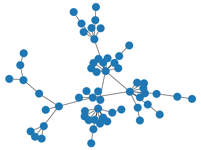
(a) $k=1$

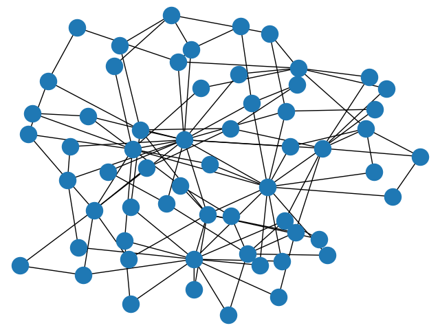
(b) $k=2$

Figure 1: Exemplar Barabási-Albert graphs with $k=1$ and $2$.

We consider initial resource distributed across the graph based on a Boltzmann distribution of the eigencentralities $\hat{c}_{i}$, in which

$$P_{i}(T)=P_{t}\frac{\exp(\hat{c}_{i}T)}{\sum_{\forall i}\exp(\hat{c}_{i}T)}\enspace,$$ (5)

where $T$ is the resource temperature, and $P_{t}$ is the total resource for a team. At zero temperature all resources are distributed evenly. Increasingly positive temperatures bias the resource distribution towards nodes with higher eigencentralities. Negative temperatures biases towards nodes with lower eigencentralities. We use eigencentralities $\hat{c}$ rather than centralities (described in Eq. (4)) due to their ability to better capture how a node is situated within the broader graph, rather than just its neighbours.

III Game Theory Solution Concepts

Solutions to coupled nonlinear differential equations like the coupled system of Eqs. (1) and (II) are readily achievable through standard numerical methods. However, while such solutions are possible for any $\Phi$, to properly understand organisational dynamics it is important to understand how a team should position itself within $\Phi$ if it is playing rationally—a concept that can only be studied through game theory. With its inherent adversarial nature, our solution concept assumes each player is playing rationally to maximise its utility.

We therefore advance a previously developed framework [29, 11], in which the (non-networked) BKL engagement can be classified as a two-player, zero-sum, strategic game, where each player is a rational and strategic decision maker. Though the strategy choices may be across numerous variables of the model (resource number, the topology, or the couplings) here we select the frustration parameter as reflecting the deliberate choice by teams how far ahead of the adversary decision ‘OODA’ cycle [30] they are attempting to operate at different points in time. Again, nonlinear dynamics may deny them their selected strategy. Within this context, for given sets of networked teams of agents $\mathcal{R},\mathcal{B}$, the frustration $\Phi$ is parameterised as

$$\Phi_{ij}(t)=\begin{cases}\phi_{k}&\text{ if }i,j\in\mathcal{B}\\ \psi_{k}&\text{ if }i,j\in\mathcal{R}\\ 0&\text{ otherwise },\end{cases}$$ (6)

where the components $\phi_{k}\in[0,\pi]$ and $\psi_{k}\in[0,\pi]$ represent the phase offsets employed by each player at discrete time-steps, $t\in[k\delta_{t},(k+1)\delta_{t}]$ for $k\in[0,\frac{T_{f}}{\delta_{t}}]$. Restricting $\phi$ and $\psi$ to changing at fixed temporal points facilitates computational tractability and deployment of exact game-theoretic solvers. Moreover, as the Networked BKL dynamics broadly exhibit exponential resource decay, introducing a finite game horizon $t\in[0,T]$ ensures that computing resources are focused upon the portions of the game which impact the final resource distribution.

At finite time horizon $T_{f}$, the game concludes. The resulting end-state of the NBKL system quantifies the game outcome for the players who each optimise for

$$U_{B}(S_{B},S_{R})=P_{B}(S_{B},S_{R})-P_{R}(S_{B},S_{R}),$$ (7)

$$U_{R}(S_{B},S_{R})=P_{R}(S_{B},S_{R})-P_{B}(S_{B},S_{R}),$$ (8)

where $P_{R}$ and $P_{B}$ are the aggregate populations of each team, which depend upon player strategies/actions via the NBKL dynamics, and $S_{B}$ and $S_{R}$ represent the vectors of strategy choices across all decision points—the values of $\phi_{k}$ for $\mathcal{B}$ and $\psi_{k}$ for $\mathcal{R}$.

Each player chooses their respective strategy vector such that their behaviour follows the Nash-Equilibria (NE), which is the set of player strategies (and utilities) where no player gains deviating from their strategy when all other players also follow their own NE. This corresponds to a fixed point at the intersection of players’ best responses (see Definition 3.22 of Başar [31]). However, pure-strategy NE may not exist in games like this. It is then natural to consider the security strategies of players, which ensure a minimum performance. Also known as min-max and max-min strategies, these strategies allow each player to establish a worst-case bound on minimum outcome [32]. Due to both the low-likelihood of repeated replay for NBKL scenarios and the computational cost of solving the underlying systems at large scales, we focus on pure strategies in contrast to probabilistic mixed strategies.

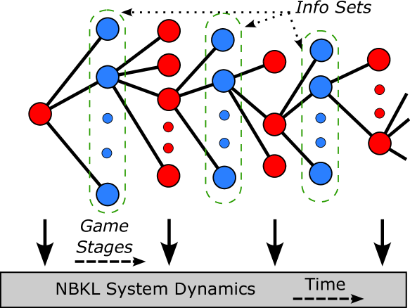
Figure 2: A game tree depicting discrete decisions of red and blue players (game stages) and the evolution of the NBKL dynamics. The information-sets apply across all actions so both players must act concurrently at each stage of the game.

Constructing game theoretic solutions is made possible through Nash Dominant Game Pruning [29], which explores the game recursively, with utilities back-propagated up the game tree from the leaves. In contrast to a search over the full game tree, the Nash Dominant approach identifies action pairs $(\phi_{k},\psi_{k})$ that are strategically dominated—that will not correspond to the equilibrium state—and truncates subsequent exploration over the game tree. This truncation occurs by identifying if any row or column would not be picked by its corresponding player because a utility along that axis is smaller/larger than the minimum/maximum observed value along a row or column. If this is observed, any sub-games that stem from decisions along an incompletely resolved row or column can be truncated.

IV Results

We now numerically solve NBKL games, considering scenarios where each team uses either its highest or lowest centrality nodes at the adversarial surface. Each team can choose from $4$ distinct values of frustration parameter at $4$ decision points in time, resulting in a game tree with $65,536$ leaf nodes. To ensure that these games are both deterministic and balanced both teams use the same fixed Barabási-Albert graph of $100$ nodes.

To examine the role of centrality in game outcomes and the decision making process, we vary across temperature values —following Eq. (5)—to control initial distribution of resources across the nodes. We consider different scenarios for the adversarial surface: both sides using the three highest centrality nodes as their adversarial surface, the asymmetric three Blue highest-vs-three Red lowest case, and both using the three lowest. Within the adversarial surface we consider when each three nodes are individually arrayed against one of the other side, “1-vs-1”, and where the three form a complete internal graph against the opposition three, “3-vs-3”. Lastly, we analyse by temperature the degree to which players reposition their actions, namely dynamically adjust the frustration $\Phi$ – how much they adjust attempting to be ahead of the decision-cycle of the adversary in the Nash Equilibrium – over the game dynamics.

IV.1 High vs High Centrality

We begin by focusing upon the case where both players use their highest centrality nodes to compete against one another, the results of which can be seen in Fig. 3. Each point in the heatmap represents the utility at a Nash equilibrium for a specific variation by both teams of their frustration parameters at discrete points in time, to achieve decision advantage. The top row represents the $BA(1)$ graph, bottom row $BA(2)$; left column is 1-vs-1, and right 3-vs-3.

Across all these we see a characteristic diagonal axis of stalemate, with Blue dominating above and Red below the diagonal. Thus, a team prevails when it concentrates resources at the low-centrality nodes of the graph if the other side elects to concentrate at high-centrality. Thus Nash dominance is achieved if concentration is away from the nodes being used for adversarial interactions; resources must be initially in reserve at the periphery if the hubs are the focus of competition.

However, while the broad morphology of the diagonal stalemate is ubiquitous, the finer detail depends upon the internal connectivity within the graph and adversarial surface. While both $BA(2)$ graphs share similar behaviours, the $3$-vs-$3$ conflict scenario deviates around the diagonal when both players temperatures at the extreme top corner. The sign flip in the outcomes is numerically small, but suggests that more interlinked team structures offer opportunity for success with an “all-in” at the point of the fight.

The $BA(1)$ graphs show contrasting structures between the $1$-vs-$1$ and $3$-vs-$3$ scenarios. The latter differs from all three cases here in its uniformity across temperature values.

These structural differences are repeated in Fig. 4, showing the proportion of repositioning in $\Phi$. The stalemate diagonal is evident, and where the utility heatmaps show variability across temperature, we observe less repositioning in $\Phi$. In contrast the more uniform result in utilities for $BA(1)$ and 3-vs-3 coincides with more repositioning of $\Phi$ during the dynamics. Overall, this suggests that for sparser graphs and higher connectivity in the adversarial surface greater agility in decision-state enables more effective manoeuvre of reserves into the competition. In the remaining discussion we will therefore identify high repositioning of $\Phi$ with agility.

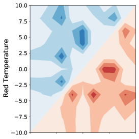
(a)

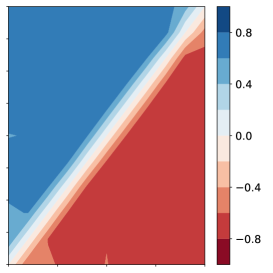
(b)

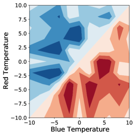
(c)

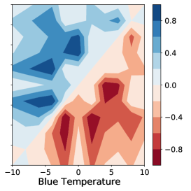
(d)

Figure 3: Security Strategy Utilities (from the perspective of the Blue player) as a function of initial resource concentration temperature, where both players engage using their $3$ highest centrality nodes. The first and second rows respectively represent $BA(1)$ and $BA(2)$ graphs, while the first and second columns represent $3$ individual $1$-vs-$1$ and a complete $3$-vs-$3$ conflict respectively.

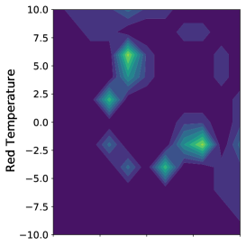
(a)

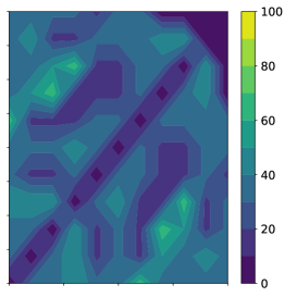
(b)

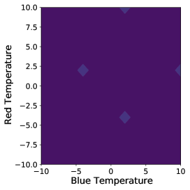
(c)

(d)

Figure 4: Percentage ratio of repositioning actions taken by both players during the Nash Equilibrium policy, relative to the maximum possible repositioning actions, consistent with Fig. 3.

IV.2 High vs Low Centrality

In the asymmetric case of Blue high- against Red low-centrality the diagonal symmetry disappears, as seen in Fig. 5. Nash dominance is consistently achieved by the high-centrality team when it concentrates resources at high-centrality nodes, namely at the adversarial surface. For the $BA(1)$ graph, the low-centrality team should also centralise its resources at its low-centrality nodes on the adversarial surface. Neither side gains from reserving resource, a consequence of the structural asymmetry between the two sides. In particular, we see that however much Red seeks to concentrate at low-centrality nodes, Blue can always initially concentrate more at its high-centrality nodes. Thus, Blue seeks to overwhelm through structural superiority, and Red cannot afford to hold back because of structural inferiority. For asymmetry, committing all-in is important to exploit resource advantage or mitigate it when lacking superior numbers at the point of the fight. The only exception to this is the occurrence of discrete poles in the $BA(1)$ 3-vs-3 case, suggesting local deviations within the random structure for intermediate initial resource distributions. These morphological sensitivities persist with different random seed for graph generation, and the number of nodes within each team’s graph. This indicates that these behaviours are a property of variability within the bulk characteristics of the graph, rather than just its finer structure.

In contrast to the High vs High (and, as we will establish forthwith the Low vs Low) scenario, the most highly polarised results are not correlated with the highest agility behaviours shown in Fig. 6. This, alongside the broad similarities between the $3$ $1$-vs-$1$ and $3$-vs-$3$ conflict suggests that the structural asymmetry of the High vs Low scenario is a structural factor that cannot be overcome by the agility of the players.

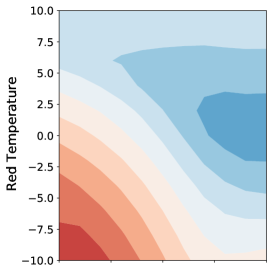
(a)

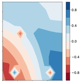
(b)

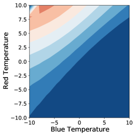
(c)

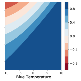
(d)

Figure 5: Security Strategy Utilities (from the perspective of the Blue player) as a function of initial resource concentration temperature, where the Blue player is using their highest centrality nodes against the lowest centrality Red nodes. The panels repeat the arrangement of Fig.3

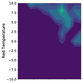
(a)

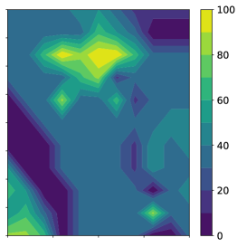
(b)

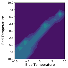
(c)

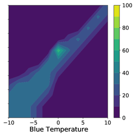
(d)

Figure 6: Percentage ratio of repositioning actions taken by both players during the Nash Equilibrium policy, relative to the maximum possible repositioning actions, consistent with Fig. 5.

IV.3 Low vs Low Centrality

When both players use their $3$ low-centrality nodes (graph periphery) for the adversarial surface, Fig. 7, we see yet another variation in behaviours. For $BA(1)$, results are inverted across the diagonal, relative to the High vs High scenario. Here then Nash dominance is achieved by the low-centrality team when it concentrates resources at the high centrality nodes, now away from the adversarial surface. Effectively, the limited paths to and narrowness of the bottleneck at the point of engagement requires that reserves be distributed. In the $BA(2)$ case we are back to the High-High case, with players incentivised to draw all their resources to the adversarial surface; more paths allow closer concentration to the engagement. In the 1-vs-1 case we see another example of isolated poles, a product of the inherently nonlinear chaotic dynamics with greater connectivity, again repeated with different random seed.

Inspecting the agility across these cases, Fig. 8 shows broad similarities to Fig. 4, in that the extrema of the Nash Equilibrium utilities correlate to the parts of the temperature space in which the players are more agile. The exception is the $BA(1)$ 1-vs-1 result where the player repositioning is consistent with higher utility. As the most topologically constrained case, this shows that agility in seeking decision-advantage provides for higher utility.

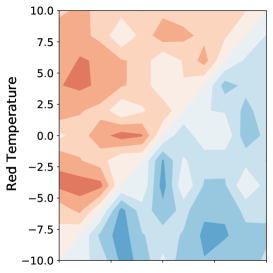
(a)

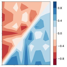
(b)

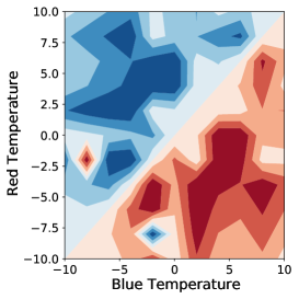
(c)

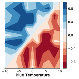
(d)

Figure 7: Security Strategy Utilities (from the perspective of the Blue player) as a function of initial resource concentration temperature, where both players engage in conflict using their $3$ lowest centrality nodes.The panels repeat the arrangement of Fig. 3.

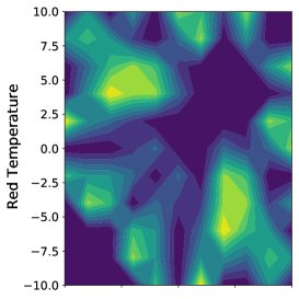
(a)

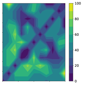
(b)

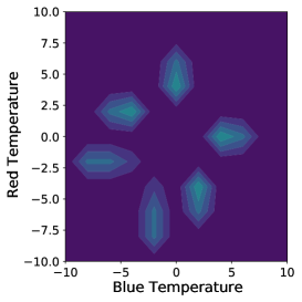
(c)

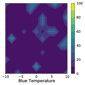
(d)

Figure 8: Percentage ratio of repositioning actions taken by both players during the Nash Equilibrium policy, relative to the maximum possible repositioning actions, consistent with Fig. 7.

V Conclusion

Analysis of adversarial team interactions modelled as the Networked Boyd-Kuramoto-Lanchester equations through a game theoretic lens yields insights into the role of network topology in ’victory’ or ’defeat’. By testing scale-free graphs with a characteristic hub-periphery topology, we were able to study the impact of structural changes in terms of the interlinking of teams, and their resource distributions. In the case of sparsely connected teams, we find that initial resources should be held in reserve, unless there is an asymmetry in the connectivity of agents at the focus of the engagement. If the hub is that point against the other team’s periphery, then the former team must exploit that advantage. Concomitantly, for the team engaging with its periphery concentrating resource elsewhere than at those nodes makes a bad situation worse. However, as the density of the connections within the team graph increases, there is a need to transition towards greater resource centralisation at the point of engagement except when both teams employ their hub nodes at the adversarial surface. These results represent Nash equilibria in decision-advantage in relation to the other, modelled by the frustration, where the nonlinearity of the Kuramoto-Lanchester model captures the complexity of resource competition in networked organisations.

We have seen that across the scenarios there are cases where agility in that decision-state over time contributes to the utility outcome. In essence, structure dominates agility is less consequential; when structure is sparse then agility becomes a significant mechanism for achieving success. We have identified these outcomes from a single graph instance; future work will systematically classify this over larger ensembles.

This work demonstrates that resource apportionment should be considered in parallel with structural designs of organisations locked in competition with an opponent and agile decision-making. That such insights are able to be gleaned from the combination of game theory and nonlinear dynamics indicates the value of such sociophysical modelling in a variety of contexts, including military strategy, business marketing strategy and cyber-security, to name but a few.

References

- Schelling [1958] T. C. Schelling, The Strategy of Conflict. Orospectus for a Reorientation of Game Theory, Journal of Conflict Resolution 2, 203 (1958).
- Raquel et al. [2007] S. Raquel, S. Ferenc, C. Emery Jr, and R. Abraham, Application of Game Theory for a Groundwater Conflict in Mexico, Journal of environmental management 84, 560 (2007).
- Berner et al. [2019] C. Berner, G. Brockman, B. Chan, V. Cheung, P. Debiak, C. Dennison, D. Farhi, Q. Fischer, S. Hashme, C. Hesse, et al., DOTA 2 with Large Scale Deep Reinforcement Learning, arXiv preprint arXiv:1912.06680 (2019).
- Vinyals et al. [2019] O. Vinyals, I. Babuschkin, W. M. Czarnecki, M. Mathieu, A. Dudzik, J. Chung, D. H. Choi, R. Powell, T. Ewalds, P. Georgiev, et al., Grandmaster Level in StarCraft II using Multi-Agent Reinforcement Learning, Nature 575, 350 (2019).
- Halevy [2008] N. Halevy, Team Negotiation: Social, Epistemic, Economic, and Psychological Consequences of Subgroup Conflict, Personality and Social Psychology Bulletin 34, 1687 (2008).
- Karabiyik et al. [2020] T. Karabiyik, A. Jaiswal, P. Thomas, and A. J. Magana, Understanding the interactions between the Scrum Master and the Development Team: A Game-Theoretic approach, Mathematics 8, 1553 (2020).
- Golestani et al. [2021] N. Golestani, E. Arzaghi, R. Abbassi, V. Garaniya, N. Abdussamie, and M. Yang, The Game of Guwarra: A Game Theory-based Decision-Making framework for Site Selection of Offshore Wind Farms in Australia, Journal of Cleaner Production 326, 129358 (2021).
- Kuramoto [2003] Y. Kuramoto, Chemical Oscillations, Waves and Turbulence (Courier Corporation, 2003).
- Boyd [1987] J. Boyd, A Discourse on Winning and Losing. Maxwell Air Force Base, AL:Air University Library Document No. M-U 43947, Briefing slides (1987).
- Osinga [2013] F. Osinga, ‘Getting’ A Discourse on Winning and Losing: A Primer on Boyd’s ‘Theory of Intellectual Evolution’, Contemporary Security Policy 34:3, 603 (2013).
- Demazy et al. [2018] A. Demazy, A. Kalloniatis, and T. Alpcan, A Game-Theoretic Analysis of the Adversarial Boyd-Kuramoto Model, in International Conference on Decision and Game Theory for Security (Springer, 2018) pp. 248–264.
- Zuparic et al. [2021] M. Zuparic, M. Angelova, Y. Zhu, and A. Kalloniatis, Adversarial Decision Strategies in Multiple Network Phased Oscillators: The Blue-Green-Red Kuramoto-Sakaguchi model, Communications in Nonlinear Science and Numerical Simulation 95, 105642 (2021).
- Lanchester [1916] F. W. Lanchester, Aircraft in Warfare: The Dawn of the Fourth Arm (Constable and Company Ltd, London, 1916).
- MacKay [2006] N. J. MacKay, Lanchester Combat Models, arXiv preprint math/0606300 (2006).
- Jin-Jiang et al. [2011] Y. Jin-Jiang, W. Yong, and W. Xian-Yu, Modeling and Simulation of Lanchester Equation based on Game Theory, in 2011 International Conference on Business Management and Electronic Information, Vol. 4 (IEEE, 2011) pp. 212–214.
- Kalloniatis et al. [2021] A. C. Kalloniatis, K. Hoek, M. Zuparic, and M. Brede, Optimising Structure in a Networked Lanchester Model for Fires and Manoeuvres in Warfare, Journal of the Operational Research Society 72, 1863 (2021), https://doi.org/10.1080/01605682.2020.1745701 .
- Ahern et al. [2021] R. Ahern, M. Zuparic, K. Hoek, and A. Kalloniatis, Unifying Warfighting Functions in Mathematical Modelling: Combat, Manoeuvre, and C2, Journal of the Operational Research Society 0, 1 (2021), https://doi.org/10.1080/01605682.2021.1956379 .
- Kondakov and Guleva [2022] M. V. Kondakov and V. Y. Guleva, Dynamics of Multiagent Reinforcement Learning Compared to Synchronisation Dynamics of Kuramoto Oscillators, Procedia Computer Science 212, 1 (2022).
- Yin et al. [2010] Z. Yin, D. Korzhyk, C. Kiekintveld, V. Conitzer, and M. Tambe, Stackelberg vs. Nash in Security Games: Interchangeability, Equivalence, and Uniqueness., in AAMAS, Vol. 10 (2010) p. 6.
- Skinner [1988] D. W. Skinner, Airland battle doctrine, Center for Naval Analyses, Professional Paper 463, 1 (1988).
- Moorthy [2014] S. Moorthy, Marketing applications of game theory, in Game Theory and Business Applications, edited by K. Chatterjee and W. Samuelson (Springer US, Boston, MA, 2014) pp. 81–101.
- Zuparic et al. [2023] M. Zuparic, S. Shelyag, M. Angelova, Y. Zhu, and A. Kalloniatis, ‘friend or Foe’ and Decision Making Initiative in Complex Conflict Environments, Plos one 18, e0281169 (2023).
- Albert and Barabási [2002] R. Albert and A.-L. Barabási, Statistical Mechanics of Complex Networks, Reviews of Modern Physics 74, 47 (2002).
- Barabási et al. [2003] A.-L. Barabási et al., Emergence of Scaling in Complex Networks, Handbook of graphs and networks , 69 (2003).
- Song et al. [2010] C. Song, T. Koren, P. Wang, and A.-L. Barabási, Modelling the Scaling Properties of Human Mobility, Nature physics 6, 818 (2010).
- Aymanns et al. [2017] C. Aymanns, J. Foerster, and C.-P. Georg, Fake News in Social Networks, arXiv preprint arXiv:1708.06233 (2017).
- Shah et al. [2020] C. Shah, N. Dehmamy, N. Perra, M. Chinazzi, A.-L. Barabási, A. Vespignani, and R. Yu, Finding Patient Zero: Learning Contagion Source with Graph Neural Networks, arXiv preprint arXiv:2006.11913 (2020).
- Li et al. [2009] P. Li, M. Zhang, Y. Xi, and W. Cui, Why organizational networks in reality do not show scale-free distributions, Comput Math Organ Theory , 169 (2009).
- Cullen et al. [2022] A. C. Cullen, T. Alpcan, and A. C. Kalloniatis, Adversarial Decisions on Complex Dynamical Systems using Game Theory, Physica A: Statistical Mechanics and its Applications 594, 126998 (2022).
- Kalloniatis and Zuparic [2016] A. Kalloniatis and M. Zuparic, Fixed Points and Stability in the Two–Network Frustrated Kuramoto Model, Physica A: Statistical Mechanics and its Applications 447, 21 (2016).
- Başar and Olsder [1999] T. Başar and G. J. Olsder, Dynamic Noncooperative Game Theory, 2nd ed. (Philadelphia, PA: SIAM, 1999).
- Leyton-Brown and Shoham [2008] K. Leyton-Brown and Y. Shoham, Essentials of Game Theory: A Concise Multidisciplinary Introduction, Synthesis Lectures on Artificial Intelligence and Machine Learning 2, 1 (2008), https://doi.org/10.2200/S00108ED1V01Y200802AIM003 .