Multistability and chaos in SEIRS epidemic model with a periodic time-dependent transmission rate

Abstract

In this work, we study the dynamics of a SEIRS epidemic model with a periodic time-dependent transmission rate. Emphasizing the influence of the seasonality frequency on the system dynamics, we analyze the largest Lyapunov exponent along parameter planes finding large chaotic regions. Furthermore, in some ranges there are shrimp-like periodic strutures. We highlight the system multistability, identifying the coexistence of periodic orbits for the same parameter values, with the infections maximum distinguishing by up one order of magnitude, depending only on the initial conditions. In this case, the basins of attraction has self-similarity. Parametric configurations, for which both periodic and non-periodic orbits occur, cover $13.20\%$ of the evaluated range. We also identified the coexistence of periodic and chaotic attractors with different maxima of infectious cases, where the periodic scenario peak reaching approximately $50\%$ higher than the chaotic one.

Seasonality is a factor that influences many infections spread. Namely, a time-dependent transmission rate leads to a non-autonomous differential equations system, enriching the dynamics and bringing features not observed in the autonomous models. Causes beyond weather seasons, as control measures and various environmental factors, may be related to temporal variations in the transmission rate of infections. It is known that the seasonality degree is relevant to change the epidemic system dynamics, as well as the average transmissivity. In addition, some diseases have distinct seasonality, as annual (e.g., rubella and measles), biannual (e.g., chikenpox) and irregular (e.g., mumps) peaks. In a general picture, the seasonality frequency does not need to be linked to annual cycles. In this way, we investigate how the seasonality parameters affects the SEIRS model dynamics, emphasizing the role of seasonality frequency.

I INTRODUCTION

Mathematical models are a fundamental tool to understand the epidemic dynamics Keeling and Rohani (2008), where approximations are made in order to replicate the focus behavior and provide a better understanding. Several diseases present periodic outbreaks Altizer et al. (2006), that are related to non-constant transmission rates Grassly and Fraser (2006). In this way, deterministic systems with constant transmission rate is not realistic Greenhalgh and Moneim (2003). In addition to the better description of real data, the inclusion of the non-constant term leads to chaotic solutions Grenfell, Bolker, and Kleczkowski (1995). Non-autonomous epidemic models, with periodic transmission rates, make it possible to model the behavior of various seasonal diseases, and present rich dynamics Aron and Schwartz (1984); Schwartz and Smith (1983); Kuznetsov and Piccardi (1994). The chaotic solutions have connection with reported data. For example, time series of many epidemic diseases as measles Olsen and Schaffer (1990), dengue Aguiar et al. (2011), mumps London and Yorke (1973) and others Keeling, Rohani, and Grenfell (2001), can be chaotic. Such behavior is associated with the seasonality present in recurrent infections Aguiar, Stollenwerk, and Kooi (2009); Tanaka and Aihara (2013). In order to simulate the chaotic dynamic, a non-linear term is included in the equations Bjørnstad (2018); Altizer et al. (2006), which can be given, for example, by a square wave or sine function Tanaka and Aihara (2013). The implications of chaotic regimes raise relevant questions in epidemiology Rand and Wilson (1991), where a consequence of the chaotic dynamics is a reduction of forecast horizons for new outbreaks Keeling and Rohani (2008). From a mathematical modeling perspective, many of the classic epidemiological models have a compartmental structure, distributing the host population into classes according to considered stages of the disease spread evolution. Essentially, there is a compartment for the population susceptible to infection, identified by the variable $S$, in addition to another one for infectious individuals, identified by $I$. There may be several other compartments, adapting the model to the studied disease characteristics Anderson and May (1991); Gabrick et al. (2022). It is assumed these groups of individuals homogeneously distributed in the population, as well as concentrations with different contagion probabilities do not occur. Homogeneity of mean disease characteristics, such as duration of infectious and latency, is also considered. The mathematical description of a compartmental epidemiological model encompasses both: host population subdivision and transition rules between the disease stages. Secondary infections usually are described by means of an interaction term between populations in $S$ and $I$ compartments.

Since the seminal work of Kermack and McKendrick Kermack and McKendrick (1927), these models have been employed to study many diseases spread Earn et al. (2000); Aguiar, Kooi, and Stollenwerk (2008); Ho, He, and Eftimie (2019); Amaku et al. (2021); Manchein et al. (2020); Brugnago et al. (2020); Amelia et al. (2022); Dalal, Greenhalgh, and Mao (2008); Dushoff et al. (2004); Galvis et al. (2022); Mugnaine et al. (2022). Formulations closer to the original proposals do not produce chaotic dynamics Cooper, Mondal, and Antonopoulos (2020); de Souza et al. (2021); Batista et al. (2021), however inclusion of multistrain Bianco, Shaw, and Schwartz (2009) or seasonal Yi et al. (2009) terms are able to reproduce chaos in a wide parameters range. Considering a SIR seasonal forced model, Stollenwerk et al. Stollenwerk et al. (2022) investigated the dynamics of respiratory diseases, like influenza. In this case, the seasonality is related to the winter months. In their results, they found a route to chaotic dynamics via period doubling bifurcations as a function of seasonality degree, similarly to the bifurcation cascade found by Yi et al. Yi et al. (2009) in a SEIR forced model. However, in the second case, additionally to the chaotic dynamics, the authors obtained hyperchaotic solutions for some parameter ranges. Completely, they investigated the dynamical behaviour by Poincaré sections and parameter planes assessing Lyapunov exponents. Another way to enrich the dynamics is by the time dependent modullation of the transmission rate Bilal et al. (2016), where the system exhibit multistability, by the coexistence of chaotic and periodic attractors for some seasonality degrees.

Bifurcation cascades as a function of various parameters in compartmental models are found in other works. Considering a SIR forced model with multistrain, Kamo and Sasaki Kamo and Sasaki (2002) showed that the cross-immunity exerts significant influence to the dynamical behaviour. For two strain, multiples attractors coexists, from which the population can switch by the introduction of small random noise in seasonally transmission. However, the complex dynamics also is present in models with one strain. In a SEIRS seasonal forced framework, Gabrick et al. Gabrick et al. (2023) showed multistable dynamics between chaotic and periodic attractors. To evidence this, they generated hysteresis-type bifurcation diagrams as a function of the recovery and average contact rates, seasonality degree, inverse of immunity and latent periods. Numerical simulations showed coexistence of chaotic and periodic attractors depending on the parameter range. Furthermore, investigating the dynamical behaviour as function of the inverse of latent period, it is possible to associate critical transitions with tipping points Medeiros et al. (2017). Once crossed this threshold, the spread diseases becomes chaotic.

A common characteristic of the works mentioned above is a period doubling route to chaos given as function of the seasonality degree. However, the authors did not take into account the effects of varied seasonality frequency. Usually, seasonality is attributed to environmental factors and, as expected, it is very common to be related to the weather seasons throughout the year Altizer et al. (2006). These seasonal forcings lead to oscillations in the infection transmission rate, being conditioned by changes in the contact rate between infectious and susceptible individuals, the circulation of infectious agents and their infectiousness. In this study, we consider different frequencies for a seasonality function, focusing on the influence of this parameter to the system dynamics. This easing of the oscillation frequency beyond the usual seasonality, together with its amplitude, allows to model diverse disturbances in the infection spread.

Firstly, we obtain the disease-free (DFE) solution, which is defined by the infection eradication in the host population. The stability of this solution is associated with the basic reproduction ratio Anderson and May (1991) ($\mathcal{R}_{0}$). Due to the non-autonomous nature of the differential equations system that describes the model, $\mathcal{R}_{0}$ is also time-dependent and oscillate between two extremes, bounded according to seasonality degree. In the autonomous case, for $\mathcal{R}_{0}<1$ the infection is extinguished and, otherwise if $\mathcal{R}_{0}>1$, then the infection grows spreading in the host population. However, for non-autonomous epidemiological systems, this criterion is not directly applicable, requiring additional and more sophisticated evaluations Ma and Ma (2006) to determine the DFE solution stability. To analyze the system dynamics Tél and Gruiz (2006), we compute the Lyapunov spectrum along parameter planes. Our results shows a wide range of chaotic behavior in all four evaluated planes. In some regions there are shrimp-like periodic structures dos Santos et al. (2016) immersed in the chaotic bands. In addition, we find multistability. The orbit resulting from the system evolution depends on the initial conditions Feudel et al. (1996); Feudel and Grebogi (1997); Feudel (2008). Even in periodic scenarios, the predictability on the final state is hard to be determined Grebogi et al. (1983). Also, for the same parametric configurations, we highlight the coexistence of periodic and chaotic attractors in scenarios where the maximum number of infectious is higher in the periodic ones.

This article is organized as follows: In Sec. II, we explain the SEIRS model and the system formulation by its variables and parameters. After, we develop a normalized version of it and include the seasonality term, which is used throughout the study. We also present the analytical DFE solution and the time-dependent basic reproduction ratio as a function of the system parameters. In Sec. III, we present numerical results, starting with an analysis of Lyapunov exponents along parameter planes, following to attraction basins evidencing the multistability. Complementarily, we compute the proportion of initial conditions that evolve to periodic dynamics along the parameter plane formed by the average transmission rate and the seasonality frequency. Finally, Sec. IV is devoted to a brief summary of the main results and our conclusions.

II MODEL

Typically presented as a system of four coupled first-order ordinary differential equations, SEIRS model describes the disease spread in a host population subdivided into four compartments, which are identified as the dynamic variables $S$, $E$, $I$ and $R$, each corresponding to a portion of the population at different infection stages. Given in the form Rock et al. (2014); Bjørnstad et al. (2020)

$$\begin{split}\frac{dS}{dt}&=\eta N+\delta R-\left(\beta\frac{I}{N}+\mu\right)S,\\ \frac{dE}{dt}&=\beta\frac{SI}{N}-(\alpha+\mu)E,\\ \frac{dI}{dt}&=\alpha E-(\gamma+\mu)I,\\ \frac{dR}{dt}&=\gamma I-(\delta+\mu)R,\end{split}$$ (1)

this system models the population transitions between its compartments. Note that the contagion occurs only through interaction between infectious (compartment $I$) and susceptible (compartment $S$) populations. In order to obtain epidemic scenarios, it is necessary to consider an initial condition with already exposed or infected individuals. A latency interval is considered, for which a portion of the population exposed (compartment $E$) to the pathogen is not yet capable to spread the infection. Once an infectious period has elapsed, individuals in $I$ acquire temporary immunity passing to the recovered compartment ($R$), where they remain until become susceptible to infection again. The host population size is the sum $N=S+E+I+R$. An illustrative scheme of this transition dynamics between compartments is shown in Fig. 1.

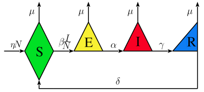
Figure 1: Illustrative scheme of the SEIRS model. The host population is divided into compartments according to the stages of infection. System (1) dynamic variables refer to states: susceptible ($S$ in green diamond); exposed ($E$ in yellow triangle); infectious ($I$ in red triangle); and recovered ($R$ in the blue triangle). Arrows connecting compartments indicate the direction of transition between them, with the respective rates. Natural mortality ($\mu$) just decreases the population allocated to each compartment.

The six parameters of the model correspond to Rock et al. (2014); Bjørnstad et al. (2020); Ma and Ma (2006): host population birth rate ($\eta$); natural death rate ($\mu$); transmission rate ($\beta$); mean latent time after the contagion ($1/\alpha$); mean infectious period ($1/\gamma$), where $\gamma$ is known as recovery rate; and mean duration of immunity consequent to infection ($1/\delta$). All parameters are non-negative real numbers.

II.1 System normalization and inclusion of seasonality

We seek a mathematical formulation of the model that allows us to study its dynamics independently of the population size. Then, without loss of generality, we perform the following transformation of variables Greenhalgh (1997); Li et al. (1999):

$$S\mapsto Ns;\leavevmode\nobreak\ \leavevmode\nobreak\ E\mapsto Ne;\leavevmode\nobreak\ \leavevmode\nobreak\ I\mapsto Ni;\leavevmode\nobreak\ \leavevmode\nobreak\ R\mapsto Nr.$$ (2)

where lowercase ones describe the normalized quantities and the total population $N>0$. Adding the four equations of the system (1), by means of algebraic manipulation, we obtain an expression for the exponential growth of the host population, being

$$\frac{dN}{dt}=(\eta-\mu)N.$$ (3)

From this fact and the relations proposed in (2), considering a generic variable $X=Nx$, we obtain

$$\frac{dX}{dt}=\frac{d(Nx)}{dt}=N\frac{dx}{dt}+x\frac{dN}{dt}.$$ (4)

Thus, we get the following transformation for the time derivatives:

$$\frac{dX}{dt} =N\left\{\frac{dx}{dt}+(\eta-\mu)x\right\},$$ (5)

$$\frac{dx}{dt} =\frac{1}{N}\left\{\frac{dX}{dt}-(\eta-\mu)X\right\},$$ (6)

where the uppercase $X$ is a non-normalized system variable and the lowercase $x$ is its normalized counterpart. Operating these transformations and, additionally, taking into account the constraint $s+e+i+r=1$, we reduce the model to a system of three equations, given by

$$\begin{split}\frac{ds}{dt}&=(\delta+\eta)(1-s)-\beta si-\delta(e+i),\\ \frac{de}{dt}&=\beta si-(\alpha+\eta)e,\\ \frac{di}{dt}&=\alpha e-(\gamma+\eta)i,\end{split}$$ (7)

whose form is identical to that arising from the constant population approximation Gabrick et al. (2023) ($\eta=\mu$).

Dynamic variables normalized according to (2) represent fractions of the host population in each compartment, such that $s,e,i,r\in[0,1]$, respecting the constraint between them. Thus, the system (7) allows simulating epidemic dynamics even in non-constant population scenarios Li et al. (1999).

In order to model a seasonal behavior of the transmission rate, we replace the constant parameter $\beta$ by the periodic function Olsen and Schaffer (1990)

$$\beta(t)=\beta_{0}\left[1+\beta_{1}\cos(\omega t)\right],$$ (8)

such that $\beta(t)$ oscillates sinusoidally around the average transmission $\beta_{0}$, with a peak-to-peak variation equal to $2\beta_{0}\beta_{1}$. Throughout the text, we refer to $\beta_{1}$ as seasonality degree. To preserve the meaning of the epidemiological model, $\beta(t)\geq 0$ is required, hence $\beta_{0}\geq 0$ and $\beta_{1}\in[0,1]$. In this study, we did not investigate the case $\beta_{0}=0$, since there is no spread of infection. Still, interested in the seasonality effects, for numerical simulations we consider $0<\beta_{1}\leq 1$ and $\omega>0$. We extend the idea of seasonality to periodic oscilations not necessarily corresponding to weather seasons, not even equivalent to integer multiples or submultiples of one year. Here, we use this term in a broader sense, referring to periodic oscillating transmission rates with any frequency.

II.2 Disease-free equilibrium

Disease-free equilibrium is so named to signify the disease disappearance in the host population. Assuming the fixed point condition

$$\frac{ds}{dt}\bigg{|}_{P_{\rm DFE}}=\frac{de}{dt}\bigg{|}_{P_{\rm DFE}}=\frac{di}{dt}\bigg{|}_{P_{\rm DFE}}=0,$$ (9)

at the point $P_{\rm DFE}(s_{*},e_{*},i_{*})$ to the system (7), we can obtain the DFE solution Anderson and May (1991) directly solving the equations

$$0 =(\delta+\eta)(1-s_{*})-\beta s_{*}i_{*}-\delta(e_{*}+i_{*}),$$ (10)

$$0 =\beta s_{*}i_{*}-(\alpha+\eta)e_{*},$$ (11)

$$0 =\alpha e_{*}-(\gamma+\eta)i_{*}.$$ (12)

We have that $s_{*}$, $e_{*}$ and $i_{*}$ are coordinates of the fixed point, therefore constant, and $\beta=\beta(t)=0$ if and only if $\beta_{1}=1$ and $t=(2k+1)\pi/\omega$, with $k\in\mathbb{Z}$ and $\beta_{0},\omega>0$. Combining these facts with both Eqs. (10) and (11) implies $s_{*}i_{*}=0$ and results $e_{*}=i_{*}=0$ in Eqs. (11) and (12), indicating the infection extinction. As for $s_{*}$, there are two distinct cases: the first for $\delta+\eta>0$, which gives $s_{*}=1$ in Eq. (10); the second occurs if $\delta=\eta=0$, in this case $s_{*}\in[0,1]$ depends on the initial conditions. The second case is more restrictive: if $\eta=0$ the model does not consider births and the population in non-normalized system (1) decays exponentially with the rate $\mu$, according to Eq. (3); while $\delta=0$ represents that infected individuals acquire permanent immunity after the infectious period, reducing the system to a SEIR model. Note that for $\beta$ as a function of time, DFE is the only fixed-point solution.

The stability of this solution is related to the basic reproduction ratio $\mathcal{R}_{0}$ Anderson and May (1991). For autonomous systems, this is a simple linear stability analysis based on the eigenvalues of the system’s Jacobian matrix calculated in the DFE point. However, in this non-autonomous case $\mathcal{R}_{0}$ is time dependent and the eradication of infection may depend of the maximum value $\max_{t}\left\{\mathcal{R}_{0}(t)\right\}$ or, specifically, related with the basic reproduction ratio obtained for the long-term average system Ma and Ma (2006).

II.3 Basic Reproduction Ratio

The contagion rate is associated with the prevalence or decline, and consequent future disappearance, of the infection in a host population. The system evolution to any of these scenarios is determined by the basic reproduction ratio, which, for the normalized SEIRS model according to Eqs. (7), is given by

$$\mathcal{R}_{0}=\alpha\beta(t)/\left[(\alpha+\eta)(\gamma+\eta)\right],$$ (13)

in the same way as the autonomous SEIRS Rock et al. (2014); Bjørnstad et al. (2020), but including an explicit time dependency in $\beta(t)$. $\mathcal{R}_{0}$ oscillates periodically in the range

$$\mathcal{R}_{0}^{-}\leq\mathcal{R}_{0}\leq\mathcal{R}_{0}^{+},$$ (14)

being the edge values defined as

$$\mathcal{R}_{0}^{\pm}\coloneqq\frac{\alpha\beta_{0}(1\pm\beta_{1})}{(\alpha+\eta)(\gamma+\eta)}.$$ (15)

We said that $\mathcal{R}_{0}$ is strictly greater than unity when $\mathcal{R}_{0}^{+}\geq\mathcal{R}_{0}^{-}>1$ and, on the other hand, refer it to by strictly less than unity if $\mathcal{R}_{0}^{-}\leq\mathcal{R}_{0}^{+}<1$. For autonomous compartmental epidemiological models, it is known that $\mathcal{R}_{0}<1$ leads to eradication of infection Bjørnstad (2018). However, since the system is non-autonomous, specifically with the transmission rate given as a function of time, a sufficient condition for convergence to the DFE solution is the long-term basic reproduction ratio $\overline{\mathcal{R}}_{0}<1$, which is calculated over the long-term average of the system evolution Ma and Ma (2006). Also, the point $P_{\rm DFE}$ is asymptotically stable if $\mathcal{R}_{0}^{+}<1$, i.e., verifying the parameters relation $\beta_{0}(1+\beta_{1})<(\alpha+\eta)(\gamma+\eta)/\alpha$.

II.4 Around endemic equilibrium

The autonomous SEIRS model, with $\beta\equiv\beta_{0}$ (equivalent to $\beta_{1}=0$ in Eq. (8)), presents a second equilibrium state, denoted by endemic equilibrium point $P_{\rm EE}(s_{\rm e},e_{\rm e},i_{\rm e})$, in which there is no extinguishes the infection in the host population Rock et al. (2014). In the non-autonomous case addressed here, the trajectories can oscillate around this point. We illustrate this behavior in Fig. 2. Arises from the fixed point condition, we obtain

$$s_{\rm e}=\frac{1}{\mathcal{R}_{\rm c}};\leavevmode\nobreak\ \leavevmode\nobreak\ e_{\rm e}=\frac{\gamma+\eta}{\alpha\beta_{0}}\varepsilon;\leavevmode\nobreak\ \leavevmode\nobreak\ i_{\rm e}=\frac{\varepsilon}{\beta_{0}},$$ (16)

where $\mathcal{R}_{\rm c}$ is the constant basic reproduction ratio, with $\beta\equiv\beta_{0}$ in Eq. (13), and

$$\varepsilon\coloneqq\frac{(\delta+\eta)(\mathcal{R}_{\rm c}-1)}{1+\frac{\mathcal{R}_{\rm c}\delta}{\beta_{0}}\left[1+\frac{\gamma+\eta}{\alpha}\right]}.$$ (17)

Note that, to recover a SEIR scheme from the system (7), simply set $\delta=0$, resulting in the $P_{\rm EE}$ for a scenario with permanent immunity Aron and Schwartz (1984). Considering the autonomous model, it is necessary $\mathcal{R}_{\rm c}>0$ for $P_{\rm EE}$ to be attractive Aron and Schwartz (1984); Schwartz and Smith (1983). To exemplify the convergence towards endemic equilibrium, we numerically integrate the autonomous system with the follow parameters: $\beta_{0}=280$, $\alpha=\gamma=100$, $\delta=2.5\times 10^{-1}$ and $\eta=2\times 10^{-2}$. In this configuration, $\mathcal{R}_{\rm c}\approx 2.799$, $s_{\rm e}\approx 3.573\times 10^{-1}$ and $i_{\rm e}\approx 1.735\times 10^{-1}$. Figure 2 shows the projection of the system’s trajectories onto the $i\times s$ plane, with $P_{\rm EE}$ in red

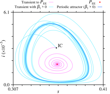
Figure 2: Trajectories evolving from ${\rm IC}$ to the attractors in the autonomous and non-autonomous cases: pink spiral converging at $P_{\rm EE}$ (red dot) in the autonomous case; light blue curve converging to the periodic attractor (blue line) in the non-autonomous case. We use a fourth order Runge-Kutta numerical integration method with a fixed step of $10^{-3}$. Transients smaller than $5\times 10^{5}$ integration steps being sufficient for the trajectories convergence to the attractors with great accuracy.

and a periodic orbit (blue line), which results from the evolution of the non-autonomous model with $\beta_{1}=0.1$ and $\omega=2\pi$. Pink and light blue curves are the transient trajectories spiraling from the initial condition ${\rm IC(0.3564,0.0032,0.0031)}$ (highlighted point) to $P_{\rm EE}$ and the periodic attractor, respectively.

III NUMERICAL RESULTS AND DISCUSSION

In this section, we numerically investigate the SEIRS model dynamics emphasizing the influence of seasonality, included according to Eq. (8). To evolve the system (7), we employ the fourth-order Runge-Kutta integration method with a fixed time step of $10^{-3}$ and consider $5\times 10^{5}$ integration steps as transient. Our simulations indicate that these settings are sufficient for the convergence of the trajectory and tangent vectors Benettin et al. (1980); Shimada and Nagashima (1979). In particular, we check the minimum transient required in parameter planes with grids of $200\times 200$ points, at $8$ transient values from $10^{3}$ to $5\times 10^{6}$ integration steps. We found that $5\times 10^{5}$ steps are enough. We also check this quantity for the other results. The time unit in the simulation is one year and the parameters have unit $\text{year}^{-1}$, except $\beta_{1}$ which is dimensionless and $[\omega]\equiv\text{rad/year}$. We vary the parameters over wide intervals, aiming to cover characteristic values of several infections, for example, measles ($\alpha=38.5$ and $\gamma=100$ ) Bai and Zhou (2012), influenza ($\alpha=228.12$ and $\gamma=125$) Cori et al. (2012), and others Lessler et al. (2009); Sartwell (1950). We start by analyzing the Lyapunov exponents on the parameter planes shown in Sub-s. III.1. Next, in Sub-s. III.2, we highlight and study the system multistability.

III.1 Lyapunov exponents analysis

In the present study, the system dynamics characterization is made mainly by the largest Lyapunov exponent. We verify that the SEIRS model, under the influence of a seasonal transmission rate, can evolve both to chaotic and periodic trajectories, depending on the parameters and initial conditions (see Sec. III.2). To investigate the effects of seasonality frequency $\omega$, with period $T=2\pi/\omega$, in the system dynamics, we compute the Lyapunov spectrum along parameter planes $[\cdot]\times\omega$, where $[\cdot]$ is a model parameter. Previously, we rewrite the system (7) in autonomous form, thus we perform the transformation $\omega t\mapsto\tau\in[0,2\pi)$ and include the respective differential equation $d\tau/dt=\omega$. The Lyapunov spectrum is obtain evolving the system and its respective linearized equations using the algorithm described by Wolf et al Wolf et al. (1985) and the exponents sorted in descending order: $\lambda_{1}\geq\lambda_{2}\geq\lambda_{3}\geq\lambda_{4}$. We adopt the initial condition $(s_{0},e_{0},i_{0},\tau_{0})=(0,999,0,0,001,0)$ and consider $10^{6}$ integration steps, after discarding the transient. Without prejudice, throughout the text $\tau_{0}=0$ will be omitted.

We analyze four parameter planes calculated on uniform grids of $1000\times 1000$ points, displayed in Figs. 3 and 4. Transmissivity oscillation frequency is on the horizontal axis, which is evaluated in the range $0<\omega\leq 6\pi$. The two largest Lyapunov exponents are represented in color: chaotic regions with $0<\lambda_{1}\leq 1.2$ (gradient from yellow to red); in periodic ones ($\lambda_{1}=0$) it shows $-1\leq\lambda_{2}<0$, starting from white ($\lambda_{2}=-1$), passing through shades of cyan to black color ($\lambda_{2}=0$).

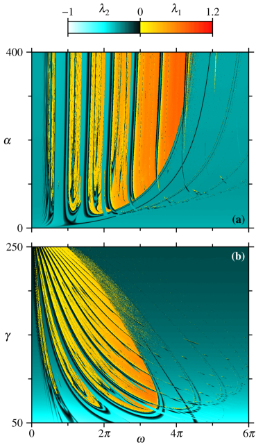
Figure 3: Parameter planes discretized in uniform grids of $1000\times 1000$ points. Lyapunov exponents in color, according to legend. Where $\lambda_{1}=0$, we display $\lambda_{2}$. Chaotic regions in the gradient from yellow to red, periodic ones in cyan shades. Horizontal axis shows the seasonality frequency. (a) Inverse of latent period on vertical axis. Intervals of chaotic regions in bands approximately parallel to the $\alpha$ axis reveal the greater relevance of $\omega$ in the system evolution. (b) Recovery rate on the vertical axis. The arrangement of the chaotic bands shows $\gamma$ as a determining factor for the dynamics. Shrimp-like periodic structures close to $\alpha=\gamma=100$ for the frequences $\omega\approx\pi$ and $\omega\approx 2\pi$.

Figure 3 illustrates two planes formed by combining $\omega$ with typical epidemiological model parameters. In the panel Fig. 3(a) we analyze the interval $0<\alpha\leq 400$ on the vertical axis, being fixed: $\gamma=100$, $\eta=0.02$, $\delta=0.25$, $\beta_{0}=270$ and $\beta_{1}=0.28$. With this parameter setting $0<\mathcal{R}_{0}\leq 3.455$, such that for $\alpha<0.008$ the basic reproduction ratio is strictly less than unity. In the interval $0.008<\alpha<0.021$ we have $0.563<\mathcal{R}_{0}^{-}<1$ and $\mathcal{R}_{0}^{+}>1$. Complementarily, we obtain $1<\mathcal{R}_{0}\leavevmode\nobreak\ \forall\leavevmode\nobreak\ t$ with $0.021<\alpha$ and, given the $\alpha$ axis discretization in steps of $\Delta\alpha=0.4$, in Fig. 3(a) we only observe results with the basic reproduction ratio strictly greater than unity. The evolution of the system to chaotic dynamics is predominantly determined by the seasonality frequency. Seasonal cycles of less than $6$ months lead predominantly to periodic behavior, see the wide dark cyan band from $\omega=4\pi$, with small chaotic regions inserted there. For $\omega<4\pi$ approximately vertical bands occur, revealing that latency intervals smaller than $\approx 1.3$ days, corresponding to $\alpha>280$, are of little relevance to the dynamics. Next to $\alpha=100$ and $\omega=2\pi$, there is a shrimp-like periodic structure, also seen around $\omega\approx\pi$. Such parameter values correspond to the latency $\approx 3.6$ days and seasonality with periods $T=1$ and $T=2$ years, respectively. Shrimps recurrently appear in parameter planes of paradigmatic non-linear systems Gallas (1993); Castro et al. (2007); Barrio et al. (2011); Rech (2017) from a peculiar arrangement of two saddle-node bifurcation curves and routes to chaos via period doubling Gallas (1994); Varga, Klapcsik, and Hegedűs (2020). The presence of these structures is evidence of rich dynamics and this vicinity is known to display shrimp cascades forming a repeating pattern with self-similarity Gallas (1994, 1995).

In Fig. 3(b) we show the plane $\gamma\times\omega$, with $50<\gamma\leq 250$, $\alpha=100$ and the other parameters are kept equal to those used in panel (a). For this system configuration, we calculate $\mathcal{R}_{0}>1\leavevmode\nobreak\ \forall\leavevmode\nobreak\ t$ with $\gamma<194.4$. However, in the range $194.4<\gamma\leq 250$ we have $0.777<\mathcal{R}_{0}^{-}<1$ and $\mathcal{R}_{0}^{+}>1$. Shrimp-like periodic structures are observed in the vicinity of $\omega=\pi$ and $\omega=2\pi$, with $\gamma\approx 100$. These periodic regions embedded in the chaotic bands are related to those in the $\alpha\times\omega$ plane. For the adopted parameters, it can be observed that the dynamics is more influenced by the infectious period than the latent one. For lower recovery rates, in the range $50<\gamma\leq 100$ corresponding to infectious periods between $\approx 7.3$ and $3.6$ days, chaotic bands extend to $\omega\approx 3.5\pi$. While for periods smaller than $\approx 1.5$ days, referring to $\gamma\approx 250$, the chaotic bands compress into the interval $0<\omega\leq\pi$. Thus, for small infectious periods, chaotic trajectories occur only for seasonality with $T\geq 2$ years. Similar to what is observed in panel (a), from $\omega\approx 3.5\pi$ ($T<6.9$ months) the analyzed parameters planes presents a wide range of periodic dynamics. Cyan area taken in the intervals $50<\gamma<75$ and $0<\omega\leq 6\pi$ corresponds to more stable periodic orbits, i.e. these are less sensitive to small disturbances than those obtained for higher recovery rates, notably the dark cyan region with $\gamma\rightarrow 250$.

As seen, the frequency of seasonal cycles significantly affects the SEIRS model dynamics, in addition to this factor, we highlight the effects of the mean transmission rate and the seasonality degree. Figure 4 display two planes with these parameters on the vertical axes, we set $\alpha=\gamma=100$ and the other values equal to those used in Fig. 3, being in panel (a) $\beta_{1}=0.28$ and in (b) $\beta_{0}=270$. Figure 4(a) comprises the interval $100<\beta_{0}\leq 600$ on the vertical axis, in it we see a periodic region around $\omega=2\pi$ and $\beta_{0}=300$ immersed in a chaotic band. This shrimp-like structure corresponds to that shown in Fig. 3(b). Mean transmission rate increasing ($\beta_{0}\rightarrow 600$) is associated with the occurrence of very stable periodic orbits ($\lambda_{2}<-0.5$). On the other hand, also for large transmissivities, with $300<\beta_{0}<550$ and around $\omega=4\pi$, the chaotic trajectories occur with the highest values of $\lambda_{1}$ (colors from orange to red). In the $\beta_{0}\times\omega$ plane evaluated section, the periodic bands are interspersed diagonally with the chaotic ones, such that the system evolution depends both on the mean transmission rate and on its frequency. In this range of $\beta_{0}$ the basic reproduction ratio varies between $\mathcal{R}_{0}^{-}\approx 0.720$ and $\mathcal{R}_{0}^{+}\approx 7.677$. For values of $\beta_{0}>138.944$ results $\mathcal{R}_{0}>1\leavevmode\nobreak\ \forall\leavevmode\nobreak\ t$. In the interval $100<\beta_{0}<138.944$ we get $0.720<\mathcal{R}_{0}^{-}<1$ and $\mathcal{R}_{0}^{+}>1$. Points $P_{1}(4\pi,456)$ and $P_{2}(2\pi,270)$, highlighted in Fig. 4(a), are targets of the multistability analysis shown in Sub-s. III.2.

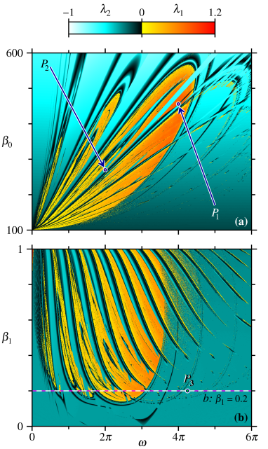
Figure 4: Parameter planes discretized in uniform grids of $1000\times 1000$ points. Lyapunov exponents in color, according to legend. Where $\lambda_{1}=0$, we display $\lambda_{2}$. Chaotic regions in the gradient from yellow to red, periodic ones in cyan shades. Horizontal axis shows the seasonality frequency. (a) Mean transmission rate on vertical axis. Diagonal periodic bands reveal the joint relevance of $\beta_{0}$ and $\omega$ to the system evolution. Highlighted points $P_{1}(4\pi,456)$ and $P_{2}(2\pi,270)$ analyzed in Sub-s. III.2 Figs. 5 and 6. (b) seazonality degree on vertical axis. Emphasized the segment $b:\leavevmode\nobreak\ \beta_{1}=0.2,\leavevmode\nobreak\ \text{whith}\leavevmode\nobreak\ 0<\omega\leq 6\pi$ (dashed line) and the point $P_{3}(4.25\pi,0.2)$, for which we analyze bifurcation diagrams and attraction basins, respectively (see Fig. 8).

Figure 4(b) illustrates the influence of $\beta_{1}$ in the SEIRS model dynamics. We consider the interval $0<\beta_{1}\leq 1$ on the vertical axis, where the transmission rate oscillates from the minimum $\beta_{0}(1-\beta_{1})$ to the maximum $\beta_{0}(1+\beta_{1})$ within one period $T$. Here $0<\mathcal{R}_{0}<5.398$, where $\mathcal{R}_{0}$ is strictly greater than unity for $0<\beta_{1}<0.629$. In the seasonality degree range $0.629<\beta_{1}\leq 1$, the edge values are $0\leq\mathcal{R}_{0}^{-}<1$ and $\mathcal{R}_{0}^{+}>1$. We observe a pattern of chaotic bands interspersed with periodic ones, similar to that displayed in Fig. 3(a). However, $\beta_{1}$ is more relevant to the dynamics than the parameter $\alpha$, increasing its influence to higher frequencies of seasonal cycles from $\omega\approx\pi$. In Sub-s. III.2 we evidence the system multistability along the segment highlighted in $\beta_{1}=0.2$ (magenta and white dashed line) and for the point $P_{3}(4.25\pi,0.2)$.

III.2 Multistability and coexistence of chaotic and periodic attractors

System (7) with periodic $\beta\equiv\beta(t)$ presents multistability Gabrick et al. (2023), i.e., different orbits can occur for a given parametric configuration, depending on the initial condition Feudel and Grebogi (1997). Given this feature, in addition to the unpredictability due to chaotic trajectories, the coexistence of chaotic and periodic attractors is observed, as well as distinct periodic orbits. Additionally to the varied dynamic behaviors, slightly different starting conditions can lead to more pronounced peaks in the infectious curve. In this subsection we investigate multistability in the model, especially for the parameter values highlighted in Sub-s III.1. All basins of attraction shown below employ a uniform grid plane discretization of $1000\times 1000$ points.

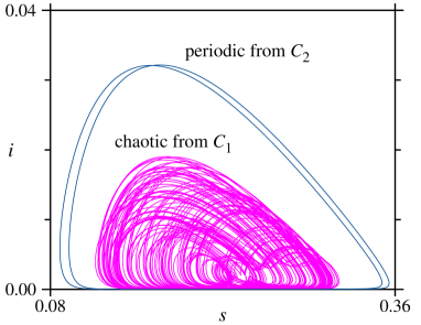
Figure 5: Plane $i\times s$ projection of attractors obtained for the point $P_{1}(4\pi,456)$, highlighted in Fig. 4(a). Chaotic attractor (magenta line) obtained from the initial condition $C_{1}=(0,990,0,001,0,009)$ and periodic one (blue line) resulting from the initial condition $C_{2}=(0.998,0.001,0.001)$. For the chaotic case the maximum value of infectious agents is $i_{\rm max}\approx 0.02$, in the periodic one it is $i_{\rm max}\approx 0.032$.

Figure 5 exhibits two attractors projected in the plane $i\times s$, one chaotic (magenta line) and other periodic (blue line), both at the point $P_{1}(\omega,\beta_{0})=P_{1}(4\pi,456)$ shown in Fig. 4(a). The chaotic attractor is generated from the initial condition $C_{1}=(0.990,0.001,0.009)$ and shows the maximum infectious population proportion $i_{\rm max}\approx 0.02$. For the periodic one we adopt the initial condition $C_{2}=(0.998,0.001,0.001)$, resulting the maximum value $i_{\rm max}\approx 0.032$. The periodic case recurrently leads to peaks of infections $\approx 50\%$ greater than the maximum observed in the chaotic situation. If, on the one hand, predictability facilitates the planning of epidemic containment protocols, on the other hand, the greater number of cases can cause harm to public health. However, both chaotic and periodic orbit present the same time average of cases $\langle{i}\rangle_{t}\approx 2.1\times 10^{-3}$

For the point $P_{2}(\omega,\beta_{0})=P_{2}(2\pi,270)$, also displayed in Fig. 4(a), we perform a scan of initial conditions and distinguish the obtained orbits between chaotic and periodic ones. To that end, we uniformly vary the initial values of infectious ($i_{0}$) and exposed ($e_{0}$). Figure 6 illustrates the plane $e_{0}\times i_{0}$ with $0<e_{0},i_{0}\leq 1$ and $s_{0}=1-(e_{0}+i_{0})$. Basins are identified in colors, where pairs $(i_{0},e_{0})$ that lead to chaotic attractors are in black and those that lead to periodic behavior are in blue. The gray region is outside the model domain. We find $\approx 53.5\%$ of valid initial conditions (outside the gray region) leading to chaotic behavior. Pairs $(e_{0},i_{0})$ that evolve to periodic attractors have a sum $0.471\leq e_{0}+i_{0}\leq 0.824$ and, consequently, $0.176\leq s_{0}\leq 0.529$. These proportions of infectious and exposed individuals are very high for the initial phase of an epidemic, even so, when it comes to dynamic analysis, these data help to understand the basins of each behavior and are especially valuable for the development of epidemic control protocols.

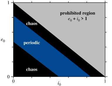
Figure 6: Plane $e_{0}\times i_{0}$ of initial conditions discretized in uniform grid of $1000\times 1000$ points. Parametric configuration of point $P_{2}(2\pi,270)$. In gray we identify the region outside the model domain. Of all evaluated valid initial conditions, $\approx 46.5\%$ evolve to periodic orbits (blue bands), the remaining $\approx 53.5\%$ leads to chaotic ones (black color).

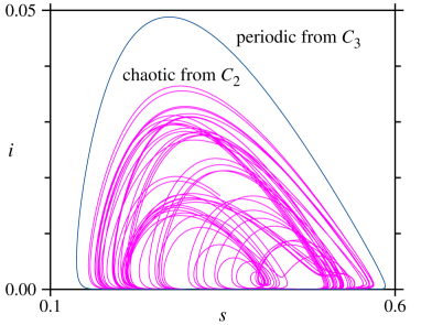
Figure 7: Plane $i\times s$ projection of attractors obtained for the point $P_{2}$. Chaotic attractor (magenta line) results from the initial condition $C_{2}=(0.998,0.001,0.001)$, periodic one (blue line) arising from $C_{3}=(0.399,0.001,0.6)$. The chaotic presents a maximum of infectious $i_{\rm max}\approx 0.037$ and the periodic one has $i_{\rm max}\approx 0.048$.

Similar to what is verified for the point $P_{1}$, for $P_{2}$ we find a periodic orbit with a higher peak of infectious agents than the chaotic one, as shown in Fig. 7. The chaotic attractor (magenta) is obtained from the same initial condition $C_{2}$ adopted in Fig. 5, the periodic one (blue) results from the condition $C_{3}=(0.399,0.001,0.6)$. Maximum infectious cases in the chaotic scenario is $i_{\rm max}\approx 0.037$, although in the periodic trajectory we have $i_{\rm max}\approx 0.048$. Both scenarios present approximately the same time average of cases, being $\langle{i}\rangle_{t}\approx 1.7\times 10^{-3}$.

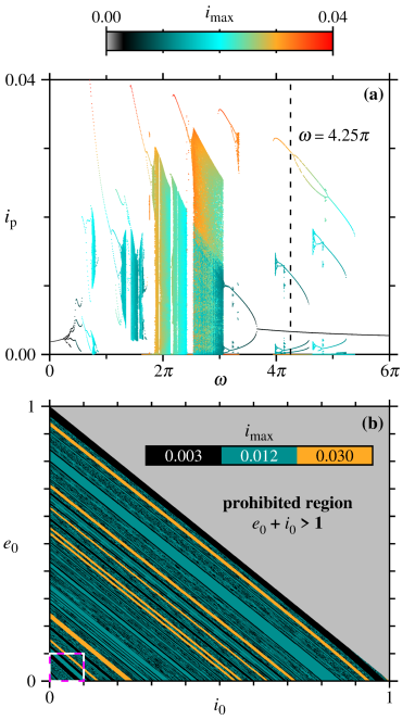
Figure 8: (a) Concatenated bifurcation diagrams of $100$ initial conditions for each $\omega$ value along segment $b_{1}$, dashed line in Fig.4(b). Horizontal axis discretized into $1000$ equidistant points. Plotted all distinct $\mathcal{I}_{k}(\omega)$. Color code for $i_{\rm max}(\omega;C_{k})$ distinguishing attractors, according Eq. (21). For $\omega=4.25\pi$ (dashed line) there are $3$ periodic attractors, this point corresponds to $P_{3}(4.25\pi,0.2)$ in Fig.4(b). (b) Basins of attraction in the initial conditions plane $e_{0}\times i_{0}$ discretized in uniforme grid of $1000\times 1000$ points, with $s_{0}=1-(e_{0}+i_{0})$ and parametric configuration for $P_{3}$. The gray region is outside of the normalized system domain. Dashed square in the bottom left corner is magnified in Fig. 9(a).

Figure 8(a) concatenates $100$ bifurcation diagrams along segment $b:\beta_{1}=0.2$, in the frequency interval $0<\omega\leq 6\pi$ uniformly discretized in $1000$ points, see dashed line in Fig.4(b). For each value of $\omega$, $100$ trajectories are generated from randomly assigned initial conditions in the interval $0<e_{0},i_{0}<1$, drawn in a uniform distribution and respecting the restriction $e_{0}+i_{0}\leq 1$, being $s_{0}=1-(e_{0}+i_{0})$. Once the transient has been discarded, we continue to evolve the system for $10^{6}$ integration steps and select the local maxima $i_{\rm p}$ (peak value) in the infectious time series over the last $7.5\times 10^{4}$ steps, equivalent to the last $75$ years in simulation. In this way, we construct a set $\mathcal{I}_{k}(\omega)$ of the local maxima in $i(t)$ curves, for given $\omega$ and the $k$-th initial condition. If there are periodic attractors, it can occur $\mathcal{I}_{j}(\omega)=\mathcal{I}_{k\neq j}(\omega)$, reducing the total amount of sets. Given the $k$-th inicial condition $C_{k}$, we have

$$i_{\rm p}(\omega;C_{k})\coloneqq i(t_{\rm p},\omega;C_{k}),$$ (18)

being

$$\frac{di}{dt}\bigg{|}_{t_{\rm p}}=0\leavevmode\nobreak\ \text{and}\leavevmode\nobreak\ \leavevmode\nobreak\ \frac{d^{2}i}{dt^{2}}\bigg{|}_{t_{\rm p}}<0.$$ (19)

Then, we define these sets as

$$\mathcal{I}_{k}(\omega)\coloneqq\left\{i_{\rm p}(\omega;C_{k}):t_{\rm p}\in\mathcal{T}\right\},$$ (20)

where $\mathcal{T}$ is the evaluation time interval. Complementarily, we identify each different set through its maximum value

$$i_{\rm max}(\omega;C_{k})\coloneqq\max\{\mathcal{I}_{k}(\omega)\}.$$ (21)

In Fig 8(a) we plot all the distinct $\mathcal{I}_{k}(\omega)$ sets. By means of $i_{\rm max}$ it is possible to distinguish different orbits that occur for the same parametric configuration, where we use the color code for such identification. This distinction is effective between periodic orbits and is also useful for highlighting points corresponding to smaller chaotic attractors from larger ones. Figure 8(a) displays the coexistence of distinct chaotic orbits in the band starting at $\omega\approx 2.5\pi$ and goes to $\omega\approx 3\pi$, where chaotic attractors occur with $i_{\rm max}\approx 0.030$ (orange dots) and others with $i_{\rm max}\approx 0.020$ (cyan and teal dots), depending on the initial conditions. For higher frequencies, we observe a vast coexistence interval of periodic attractors, as an example in $\omega=4.25\pi$ (vertical dashed line), where are $3$ periodic orbits, being these of: period $1$, with $i_{\rm max}\approx 0.003$ (black color); period $3$, with $i_{\rm max}\approx 0.012$ (teal color); and period $2$, with $i_{\rm max}\approx 0.030$ (orange color). High peaks of infectious are obtained for $\omega\approx 1.5\pi$ and $\omega\approx 0.7\pi$, where $i_{\rm p}\approx 0.04$, i.e., the local maxima in the infectious time series reach, periodically, nearly $4\%$ of the host population.

Coexistence of orbits with such a discrepancy in the maximum value of infectious, as seen in Fig. 8(a), evidencing the initial conditions influence, not only to the system dynamic regime, but also determining the system evolution to scenarios with a greater or lesser number of infected individuals, arriving at the difference in order of magnitude. Figure 8(b) displays the attraction basins of the three listed periodic attractors for $\omega=4.25\pi$, corresponding to the point $P_{3}(\omega,\beta_{1})=P_{3}(4.25\pi,0.2)$, shown in Fig. 4(b). Initial conditions on plane $e_{0}\times i_{0}$ are in the same intervals and grid configuration as in Fig. 6. The color code used to identify the $3$ different basins is similar to the one employed in the bifurcation diagram, there is a slight difference in color tone to facilitate visualization. Pairs $(i_{0},e_{0})$ that lead to period $1$ orbit (with $i_{\rm max}\approx 0.003$) are in black color; those leading to the period $3$ orbit (with $i_{\rm max}\approx 0.012$) are in teal color; and those that evolve to period $2$ orbit (with $i_{\rm max}\approx 0.030$) are in orange color. The gray region contains the pairs outside the normalized system domain (prohibited region). Notable are the alternating diagonal bands of the attraction basins. The highlight region in the bottom left corner, bounded by the white and magenta dashed box, is amplified in Fig. 9(a) followed by two magnifications, in which the self-similarity and intricate nature of the attraction basins obtained for $P_{3}$ is evident.

The succession of magnifications shown in Fig. 9 starts in the region marked in Fig. 8(b) and proceeds to scan intervals of initial conditions one order of magnitude smaller per panel, with the area covered in each successor being $10^{-2}$ times that of the previous one. Color code is the same as Fig. 8(b), identifying the $i_{\rm max}$ of the attractor resulting from each pair $(e_{0},i_{0})$. Table 1 presents the area percentage occupied by each basin of attraction for all $3$ evaluated ranges of initial conditions.

Table 1: Area percentage occupied by each basin of attraction for the $3$ evaluated regions. First column identifies the panel in Fig. 9 and the second column informs the respective range of initial conditions.

		$i_{\rm max}$
Panel	$e_{0},i_{0}\in$	$0.003$	$0.012$	$0.030$
a	$\left(0,10^{-1}\right]$	$46.75\%$	$47.78\%$	$5.47\%$
b	$\left(0,10^{-2}\right]$	$40,32\%$	$44,02\%$	$15,66\%$
c	$\left(0,10^{-3}\right]$	$32,39\%$	$65,97\%$	$1,64\%$

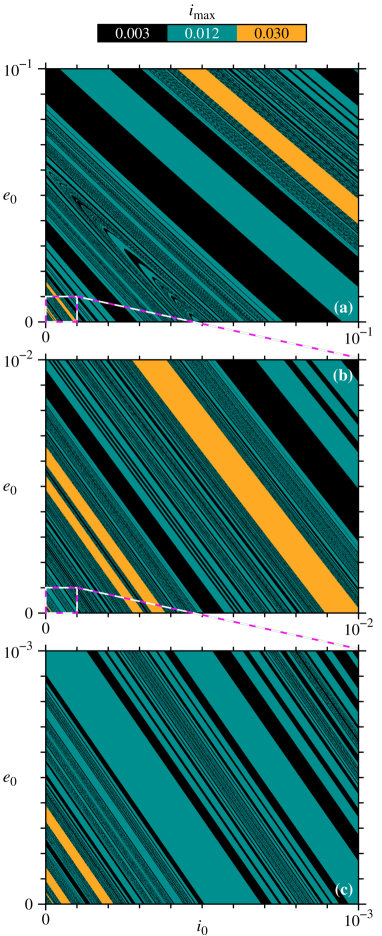
Figure 9: Attraction basins in a succession of magnifications. Axes discretized in uniform grid of $1000\times 1000$ points. Color code identifies the maximum infectious value $i_{\rm max}$ of each attractor, as defined in Eq. (21). (a) Magnification of the delimited region in Fig. 8(b), with $0<e_{0},i_{0}\leq 10^{-1}$. Box in bottom left corner enlarged on panel (b) $0<e_{0},i_{0}\leq 10^{-2}$. In turn, the highlighted box is magnified in (c) $0<e_{0},i_{0}\leq 10^{-3}$.

First, in Fig 9(a) we evaluate the initial conditions interval $0<e_{0},i_{0}\leq 10^{-1}$, where $46.75\%$ of the points lead to smallest $i_{\rm max}$ orbit and $5.47\%$ of them belong to the attraction basin of the periodic attractor with highest infectious peak. The box at the bottom left corner is enlarged in panel (b), where $0<e_{0},i_{0}\leq 0,10^{-2}$. In this region, the basin of attraction corresponding to $i_{\rm max}\approx 0.003$ occupying $40,32\%$ of the total area and highest infectious peak attractor results from $15,66\%$ of the initial conditions. Panel (c) shows the last magnification, performed in the interval $0<e_{0},i_{0}\leq 0,10^{-3}$, being $65.97\%$ of the area occupied by the basin of period $3$ attractor, with the maximum of infectious $\approx 0.012$. In this sample, only $1.64\%$ of the total area leads to $i_{\rm max}\approx 0.030$. Given the discretization and intervals of both axes in Fig. 9(c), one-point variation, being the increment of $10^{-6}$ either vertically or horizontally, represents a difference of $1$ individual in $1$ million of the host population for the initial condition of infectious or exposed. Resulting in significantly different maximum infectious values for this small change, with greater sensitivity for $e_{0}$ and $i_{0}$ of smaller orders of magnitude.

Finally, in Fig. 10 we obtain a fraction of initial conditions that result in periodic orbits for points along the parameter plane $\beta_{0}\times\omega$. We use the same intervals and parametric configuration of Fig. 4(a). For each pair $(\omega,\beta_{0})$, we draw $100$ equiprobable initial conditions in the interval $0<e_{0},i_{0}<1$, respecting the constraint $e_{0}+i_{0}\leq 1$. Similar to what is made to obtain the bifurcation diagram in Fig. 8(a), starting from the $k$-th initial condition $C_{k}$, we evolve the system by $10^{6}$ integration steps even after the transient and evaluate only the last $7.5\times 10^{4}$ trajectory points. In this section of the time series, we select the local maxima in the $s(t),\leavevmode\nobreak\ e(t)$ and $i(t)$ curves and check the periodicity with an accuracy of $10^{-6}$. Period $12$ is considered the maximum. We do not focus on determining the period of each orbit, but just identify if it is periodic or not and, subsequently, compute the fraction $\rho_{\rm per}(\omega,\beta_{0})$ of initial conditions that leads to periodic behavior.

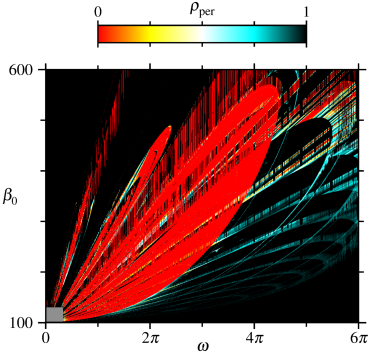
Figure 10: In colors the fraction $\rho_{\rm per}(\omega,\beta_{0})$ of the trajectories that evolve to periodic dynamics, from $100$ randomly assigned initial conditions. Parameter plane discretized in uniform grid of $1000\times 1000$ points, with $0<\omega\leq 6\pi$ and $100<\beta_{0}\leq 600$. Coexistence of periodic and non-periodic orbits ($0<\rho<1$) is observed in $13.20\%$ of the valid area. In the gray square region, the time series sampling was not enough to verify periodicity.

In the sense explained above, Figure 10 consolidates information from $100$ parameter planes, each associated with the $k$-th initial condition for every pair $(\omega,\beta_{0})$. We represent $\rho_{\rm per}$ by the color code. Pairs in this plane for which all evaluated initial conditions result in periodic orbits ($\rho_{\rm per}=1$) are in black color. The ones that $100\%$ led to non-periodic attractors ($\rho_{\rm per}=0$) are in red color. Intermediate cases are on the gradient from red to yellow ($\rho_{\rm per}=0.25$) and white ($\rho_{\rm per}=0.5$) and, on the other side, from white to cyan ($\rho_{\rm per}=0.75$) and black. In the small gray region (bottom left corner), the sample of time series are not enough to determine periodicity, or deny it, due to the high period of oscillations. Regions with some fraction of non-periodic behavior, where $\rho_{\rm per}<1$, resemble the bands of $\lambda_{1}>0$ shown in Fig. 4(a). Unlike the initial condition considered in Sub-s III.1, here the exposed initial value is not null. Furthermore, accuracy, sampling and the maximum period adopted result in some differences between this and that parameter plane.

The cyan bands in Fig. 10, as well as the small yellow regions, demonstrate the coexistence of periodic and non-periodic orbits, related to seasonality parameters. Through this assessment, we obtain only periodic orbits for $61.50\%$ of the valid area (subtracting the gray region), exclusively non-periodic along $25.30\%$ and both behaviors coexist in $13.20\%$ of the parameter plane.

IV CONCLUSION

We numerically investigated the SEIRS model dynamics under a time-dependent transmission rate. Such temporal dependence is periodic and consists of expanding the concept of seasonality, considering different periods in addition to those that synchronize with the climatic seasons. Through parameter planes combining the seasonality frequency and typical epidemiological model parameters, we evidenced the chaotic dynamics occurrence, referring to various analyses of reported data suggesting that some epidemics has chaotic behaviorLondon and Yorke (1973); Olsen and Schaffer (1990); Jones and Strigul (2021). Focusing on the transmission rate function, we highlight the coexistence of chaotic and periodic orbits for certain parametric configurations, as well as a diversity of periodic attractors. We found that chaotic orbits may present lower infectious peaks than periodic ones, even so with the same temporal average of infectious cases. Assuming it is a disease that affects humans (which is not a premiss of the model), the predictability of periodic orbits facilitates the planning of public health campaigns. On the other hand, the lowest maximum number of cases in the chaotic attractor may represent a benefit when it comes to reduce the infection spread. In terms of modeling real-world infections based on the system studied in this work, it is necessary consider the precision which the parameters can be determined, since in the parameter planes there are narrow periodic bands immersed in chaotic regions. Also, in the vicinity of the shrimp-like structures, cascades of similar periodic regions occur, entering in scales of very small parametric variations, in such a way that small changes in the parameters can lead to a drastic change in the dynamic behavior.

The system presents multistability of periodic orbits with different periods showing marked difference in the maximum infected values. By means of attraction basins, obtained for certain parametric configuration, we showed that small variations of the initial conditions can lead to different orders of magnitude of the maximum infectious agents number. Furthermore, for a wide range of frequency and average transmissivity settings, orbits of periods up to $12$ coexist with larger periods and even non-periodic ones. Those two features of the system, present chaotic dynamics and multistability, lead to challenges for proposals of epidemic control, since chaotic dynamics reduce predictability and the multistable character can lead to significantly different periodic orbits through small changes of the initial conditions. The oscilation frequency of the transmission rate proved to be relevant to the system dynamics, being one of the determining factors for the occurrence of chaos. Seasonality parameters also influence oscillations in the infectious curve in periodic scenarios, resulting in different counts of local maxima within a period. An investigation of this relationship can be carried out using isospike diagrams, however, is far from the focus of the present study, so we consider it for a future work.

DATA AVAILABILITY

The data that support the findings of this study are available from the corresponding authors upon reasonable request.

References

- Keeling and Rohani (2008) M. J. Keeling and P. Rohani, Modeling Infectious Diseases in Humans and Animals, 1st ed. (Princeton University Press, Princeton, 2008).
- Altizer et al. (2006) S. Altizer, A. Dobson, P. Hosseini, P. Hudson, M. Pascual, and P. Rohani, “Seasonality and the dynamics of infectious diseases,” Ecol. Lett. 9, 467–484 (2006).
- Grassly and Fraser (2006) N. C. Grassly and C. Fraser, “Seasonal infectious disease epidemiology,” Proc. Royal Soc. B 273, 2541–2550 (2006).
- Greenhalgh and Moneim (2003) D. Greenhalgh and I. A. Moneim, “SIRS epidemic model and simulations using different types of seasonal contact rate,” Syst. Anal. Model. Simul. 43, 573–600 (2003).
- Grenfell, Bolker, and Kleczkowski (1995) B. T. Grenfell, B. M. Bolker, and A. Kleczkowski, “Seasonality and extinction in chaotic metapopulations,” Proc. Royal Soc. B 259, 97–103 (1995).
- Aron and Schwartz (1984) J. L. Aron and I. B. Schwartz, “Seasonality and period-doubling bifurcations in an epidemic model,” J. Theor. Biology 110, 665–679 (1984).
- Schwartz and Smith (1983) I. B. Schwartz and H. L. Smith, “Infinite subharmonic bifurcation in an SEIR epidemic model,” J Math Biol 18, 233–253 (1983).
- Kuznetsov and Piccardi (1994) Y. A. Kuznetsov and C. Piccardi, “Bifurcation analysis of periodic SEIR and SIR epidemic models,” J Math Biol 32, 109–121 (1994).
- Olsen and Schaffer (1990) L. F. Olsen and W. M. Schaffer, “Chaos versus noisy periodicity: alternative hypotheses for childhood epidemics,” Science 249, 499–504 (1990).
- Aguiar et al. (2011) M. Aguiar, S. Ballesteros, B. W. Kooi, and N. Stollenwerk, “The role of seasonality and import in a minimalistic multi-strain dengue model capturing differences between primary and secondary infections: complex dynamics and its implications for data analysis,” J. Theor. Biol. 289, 181–196 (2011).
- London and Yorke (1973) W. P. London and J. A. Yorke, “Recurrent outbreaks of measles, chickenpox and mumps: I. seasonal variation in contact rates,” Am. J. Epidemiol. 98, 453–468 (1973).
- Keeling, Rohani, and Grenfell (2001) M. J. Keeling, P. Rohani, and B. T. Grenfell, “Seasonally forced disease dynamics explored as switching between attractors,” Physica D 148, 317–335 (2001).
- Aguiar, Stollenwerk, and Kooi (2009) M. Aguiar, N. Stollenwerk, and B. W. Kooi, “Torus bifurcations, isolas and chaotic attractors in a simple dengue fever model with ade and temporary cross immunity,” Int J Comput Math 86, 1867–1877 (2009).
- Tanaka and Aihara (2013) G. Tanaka and K. Aihara, “Effects of seasonal variation patterns on recurrent outbreaks in epidemic models,” J. Theor. Biol. 317, 87–95 (2013).
- Bjørnstad (2018) O. N. Bjørnstad, Epidemics: Models and Data using R, 1st ed. (Springer Cham, 2018) pp. XIII, 312.
- Rand and Wilson (1991) D. A. Rand and H. B. Wilson, “Chaotic stochasticity: A ubiquitous source of unpredictability in epidemics,” Proc. R. Soc. B 246, 179–184 (1991).
- Anderson and May (1991) R. M. Anderson and R. M. May, Infectious diseases of humans: dynamics and control (Oxford university press, 1991).
- Gabrick et al. (2022) E. C. Gabrick, P. R. Protachevicz, A. M. Batista, K. C. Iarosz, S. L. T. de Souza, A. C. L. Almeida, J. D. Szezech Jr, M. Mugnaine, and I. L. Caldas, “Effect of two vaccine doses in the SEIR epidemic model using a stochastic cellular automaton,” Physica A 597, 127258 (2022).
- Kermack and McKendrick (1927) W. O. Kermack and A. G. McKendrick, “A contribution to the mathematical theory of epidemics,” Proc. R. Soc. Lond. A 115, 700–721 (1927).
- Earn et al. (2000) D. J. D. Earn, P. Rohani, B. M. Bolker, and B. T. Grenfell, “A simple model for complex dynamical transitions in epidemics,” Science 287, 667–670 (2000).
- Aguiar, Kooi, and Stollenwerk (2008) M. Aguiar, B. Kooi, and N. Stollenwerk, “Epidemiology of dengue fever: A model with temporary cross-immunity and possible secondary infection shows bifurcations and chaotic behaviour in wide parameter regions,” Math. Model. Nat. Phenom. 3, 48–70 (2008).
- Ho, He, and Eftimie (2019) S. H. Ho, D. He, and R. Eftimie, “Mathematical models of transmission dynamics and vaccine strategies in in Hong Kong during the 2017-2018 winter influenza season,” J. Theor. Biol. 476, 74–94 (2019).
- Amaku et al. (2021) M. Amaku, D. T. Covas, F. A. B. Coutinho, R. S. A. Neto, C. Struchiner, A. Wilder-Smith, and E. Massad, “Modelling the test, trace and quarantine strategy to control the COVID-19 epidemic in the state of são paulo, brazil,” Infect. Dis. Model. 6, 46–55 (2021).
- Manchein et al. (2020) C. Manchein, E. L. Brugnago, R. M. da Silva, C. F. O. Mendes, and M. W. Beims, “Strong correlations between power-law growth of COVID-19 in four continents and the inefficiency of soft quarantine strategies,” Chaos 30, 041102 (2020).
- Brugnago et al. (2020) E. L. Brugnago, R. M. da Silva, C. Manchein, and M. W. Beim, “How relevant is the decision of containment measures against COVID-19 applied ahead of time?” Chaos Solitons Fractals 140, 110164 (2020).
- Amelia et al. (2022) R. Amelia, N. Anggriani, A. K. Supriatna, and N. Istifadah, “Mathematical model for analyzing the dynamics of tungro virus disease in rice: A systematic literature review,” Mathematics 10, 2944 (2022).
- Dalal, Greenhalgh, and Mao (2008) N. Dalal, D. Greenhalgh, and X. Mao, “A stochastic model for internal hiv dynamics,” J. Math. Anal. Appl. 341, 1084–1101 (2008).
- Dushoff et al. (2004) J. Dushoff, J. B. Plotkin, S. A. Levin, and D. J. D. Earn, “Dynamical resonance can account for seasonality of influenza epidemics,” PNAS 101, 16915–16916 (2004).
- Galvis et al. (2022) J. A. Galvis, C. A. Corzo, J. M. Prada, and G. Machado, “Modeling between-farm transmission dynamics of porcine epidemic diarrhea virus: Characterizing the dominant transmission routes,” Prev. Vet. Med. 208, 105759 (2022).
- Mugnaine et al. (2022) M. Mugnaine, E. C. Gabrick, P. R. Protachevicz, K. C. Iarosz, S. L. de Souza, A. C. Almeida, A. M. Batista, I. L. Caldas, J. D. Szezech Jr, and R. L. Viana, “Control attenuation and temporary immunity in a cellular automata SEIR epidemic model,” Chaos Solitons Fractals 155, 111784 (2022).
- Cooper, Mondal, and Antonopoulos (2020) I. Cooper, A. Mondal, and C. G. Antonopoulos, “A SIR model assumption for the spread of COVID-19 in different communities,” Chaos Solitons Fractals 139, 110057 (2020).
- de Souza et al. (2021) S. L. de Souza, A. M. Batista, I. L. Caldas, K. C. Iarosz, and J. D. Szezech Jr, “Dynamics of epidemics: Impact of easing restrictions and control of infection spread,” Chaos Solitons Fractals 142, 110431 (2021).
- Batista et al. (2021) A. M. Batista, S. L. T. de Souza, K. C. I. , A. C. L. Almeida, J. D. Szezech Jr, E. C. Gabrick, M. Mugnaine, dos G. L. Santos, and I. L. Caldas, “Simulation of deterministic compartmental models for infectious diseases dynamics,” Rev. Bras. de Ensino de Fis. 43, e20210171 (2021).
- Bianco, Shaw, and Schwartz (2009) S. Bianco, L. B. Shaw, and I. B. Schwartz, “Epidemics with multistrain interactions: The interplay between cross immunity and antibody-dependent enhancement,” Chaos 19, 043123 (2009).
- Yi et al. (2009) N. Yi, Q. Zhang, K. M. D. Yang, and Q. Li, “Analysis and control of an SEIR epidemic system with nonlinear transmission rate,” Math. Comput. Model 50, 1498–1513 (2009).
- Stollenwerk et al. (2022) N. Stollenwerk, S. Spaziani, J. Mar, I. E. Arrizabalaga, D. Knopoff, N. Cusimano, V. Anam, A. Shrivastava, and M. Aguiar, “Seasonally forced SIR systems applied to respiratory infectious diseases, bifurcations, and chaos,” Comput. math. methods , 3556043 (2022).
- Bilal et al. (2016) S. Bilal, B. K. Singh, A. Prasad, and E. Michael, “Effects of quasiperiodic forcing in epidemic models,” Chaos 26, 093115 (2016).
- Kamo and Sasaki (2002) M. Kamo and A. Sasaki, “The effect of cross-immunity and seasonal forcing in a multi-strain epidemic model,” Physica D 165, 228–241 (2002).
- Gabrick et al. (2023) E. C. Gabrick, E. Sayari, P. R. Protachevicz, J. D. Szezech Jr, K. C. Iarosz, S. L. T. de Souza, A. C. L. Almeida, R. L. Viana, I. L. Caldas, and A. M. Batista, “Unpredictability in seasonal infectious diseases spread,” Chaos Solitons Fractals 166, 113001 (2023).
- Medeiros et al. (2017) E. S. Medeiros, I. L. Caldas, M. S. Baptista, and U. Feudel, “Trapping phenomenon attenuates the consequences of tipping points for limit cycles,” Sci. Rep. 7, 42351 (2017).
- Ma and Ma (2006) J. Ma and Z. Ma, “Epidemic threshold conditions for seasonally forced SEIR models,” Math Biosci Eng 3, 161 (2006).
- Tél and Gruiz (2006) T. Tél and M. Gruiz, Modeling Infectious Diseases in Humans and Animals, 1st ed. (Chaotic Dynamics: And introduction based on Classical Mechanics, Cambridge, 2006).
- dos Santos et al. (2016) V. dos Santos, J. D. Szezech Jr, M. S. Baptista, A. M. Batista, and I. L. Caldas, “Unstable dimension variability structure in the parameter space of coupled Hénon maps,” Appl. Math. Comput. 286, 23–28 (2016).
- Feudel et al. (1996) U. Feudel, C. Grebogi, B. R. Hunt, and J. A. Yorke, “Map with more than 100 coexisting low-period periodic attractors,” Phys. Rev. E 54, 71–81 (1996).
- Feudel and Grebogi (1997) U. Feudel and C. Grebogi, “Multistability and the control of complexity,” Chaos 7, 597–604 (1997).
- Feudel (2008) U. Feudel, “Complex dynamics in multistable systems,” Int J Bifurcat Chaos 18, 1607–1626 (2008).
- Grebogi et al. (1983) C. Grebogi, S. W. McDonald, E. Ott, and J. A. Yorke, “Final state sensitivy: an obstruction to predictability,” Phys. Lett. A 99A, 415–418 (1983).
- Rock et al. (2014) K. Rock, S. Brand, J. Moir, and M. J. Keeling, “Dynamics of infectious diseases,” Rep. Prog. Phys. 77, 026602 (2014).
- Bjørnstad et al. (2020) O. N. Bjørnstad, K. Shea, M. Krzywinski, and N. Altman, “The SEIRS model for infectious disease dynamics,” Nat. Methods 17, 557–558 (2020).
- Greenhalgh (1997) D. Greenhalgh, “Hopf bifurcation in epidemic models with a latent period and nonpermanent immunity,” Math. Comput. Model 25, 85–107 (1997).
- Li et al. (1999) M. Y. Li, J. R. Graef, L. Wang, and J. Karsai, “Global dynamics of a SEIR model with varying total population size,” Math Biosci 160, 191–213 (1999).
- Benettin et al. (1980) G. Benettin, L. Galgani, A. Giorgilli, and J.-M. Strelcyn, “Lyapunov characteristic exponents for smooth dynamical systems and for Hamiltonian systems; a method for computing all of them. Part 1: Theory,” Meccanica 15, 9–20 (1980).
- Shimada and Nagashima (1979) I. Shimada and T. Nagashima, “A Numerical Approach to Ergodic Problem of Dissipative Dynamical Systems,” Prog. theor. phys. 61, 1605–1616 (1979).
- Bai and Zhou (2012) Z. Bai and Y. Zhou, “Global dynamics of an SEIRS epidemic model with periodic vaccination and seasonal contact rate,” Nonlinear Anal Real World Appl 13, 1060–1068 (2012).
- Cori et al. (2012) A. Cori, A. J. Valleron, F. Carrat, G. Scalia Tomba, G. Thomas, and P. Y. Boëlle, “Estimating influenza latency and infectious period durations using viral excretion data,” Epidemics 4, 132–138 (2012).
- Lessler et al. (2009) J. Lessler, N. G. Reich, R. Brookmeyer, T. M. Perl, K. E. Nelson, and D. A. T. Cummings, “Incubation periods of acute respiratory viral infections: a systematic review,” Lancet Infect. Dis. 9, 291–300 (2009).
- Sartwell (1950) P. E. Sartwell, “The distribution of incubation periods of infectioou disease,” Am. J. Epidemiol. 51, 310–318 (1950).
- Wolf et al. (1985) A. Wolf, J. B. Swift, H. L. Swinney, and J. A. Vastano, “Determining lyapunov exponents from a time series,” Physica D 16, 285–317 (1985).
- Gallas (1993) J. A. C. Gallas, “Structure of the parameter space of the Hénon map,” Phys. Rev. Lett. 70, 2714 (1993).
- Castro et al. (2007) V. Castro, M. Monti, W. B. P. B, J. A. Walkenstein, and E. Rosa Jr, “Characterization of the Rössler system in parameter space,” Int J Bifurcat Chaos 17, 965–973 (2007).
- Barrio et al. (2011) R. Barrio, F. Blesa, S. Serrano, and A. Shilnikov, “Global organization of spiral structures in biparameter space of dissipative systems with Shilnikov saddle-foci,” Phys. Rev. E 84, 035201 (2011).
- Rech (2017) P. C. Rech, “How to embed shrimps in parameter planes of the Lorenz system,” Phys Scr 92, 045201 (2017).
- Gallas (1994) J. A. C. Gallas, “Dissecting shrimps: results for some one-dimensional physical models,” Physica A 202, 196–223 (1994).
- Varga, Klapcsik, and Hegedűs (2020) R. Varga, K. Klapcsik, and F. Hegedűs, “Route to shrimps: Dissipation driven formation of shrimp-shaped domains,” Chaos Solitons Fractals 130, 109424 (2020).
- Gallas (1995) J. A. C. Gallas, “Structure of the parameter space of a ring cavity,” Appl Phys B-Lasers O 60, S203 (1995).
- Jones and Strigul (2021) A. Jones and N. Strigul, “Is spread of COVID-19 a chaotic epidemic?” Chaos Solitons Fractals 142, 110376 (2021).