Impact of astrophysical scatter on the Epoch of Reionization [H i]${}_{\text{21cm}}$ bispectrum

Abstract

It is believed that the first star-forming galaxies are the main drivers of cosmic reionization. It is usually assumed that there is a one-to-one relationship between the star formation rate (SFR) inside a galaxy and the host halo mass in semi-analytical/numerical modeling of large-scale ionization maps during the epoch of reionization. However, more accurate simulations and observations suggest that the SFR and ionizing luminosity in galaxies may vary considerably even if the host halo mass is the same. This astrophysical scatter can introduce an additional non-Gaussianity in the cosmological [H i]${}_{\text{21cm}}$ signal, which is already expected to have an inherent time-evolving non-Gaussianity due to reionization. Here, we have studied the impact of the scatter on the [H i]${}_{\text{21cm}}$ bispectrum using semi-numerical simulations. The scatter primarily affects small ionized regions, whereas the large ionized bubbles remain largely unaffected. Although, the fractional change in the [H i]${}_{\text{21cm}}$ bispectra due to the scatter is found to be more than a factor of $10$ at large scales ($\lesssim 1\,{\rm Mpc}^{-1}$), it is found to be statistically not significant. However, we have found the impact due to the scatter to be significant ($|\langle\Delta B\rangle/B_{\text{no-scatter}}|\sim 1$) at small scales ($k\sim 2.55$ Mpc^-1) and at $\overline{x}_{\text{H\,{i}}}\sim 0.8$. We have also found that 1000 hours of SKA1-Low like observation is unlikely to detect the signatures of the scatter at these small scales.

1 Introduction

Modeling observable summary statistics for line-intensity mapping (LIM) signals is one of the key steps to build inference frameworks to understand the poorly constrained epoch of reionization (EoR). The LIM signal corresponding to the redshifted [H i]${}_{\text{21cm}}$ emissions from the diffuse IGM (Wouthuysen, 1952; Field, 1958; Madau et al., 1997), and [C ii]${}_{158\mu\text{m}}$ (Gong et al., 2012; Silva et al., 2015; Padmanabhan, 2019; Yue & Ferrara, 2019; Murmu et al., 2021; Murmu et al., 2022; Karoumpis et al., 2022), CO (Lidz et al., 2011; Li et al., 2016; Yang et al., 2022; Moradinezhad Dizgah et al., 2023; Roy et al., 2023), Ly-$\alpha$  (Peterson & Suarez, 2012; Silva et al., 2013; Pullen et al., 2014; Mas-Ribas & Chang, 2020), [O iii]${}_{88\mu\text{m}}$ (Padmanabhan, 2023) etc. emissions from bright galaxies have been proposed as potential probes for studying the EoR. We can map the universe, and its cosmic evolution using these line emissions. In that process, one can use suitable summary statistics to infer cosmological information from these probes. Fourier-based statistics, such as the power spectrum, provide information on signal fluctuations at different length scales. Higher-order statistics, such as the bispectrum, can reveal non-Gaussian features present in the signal at multiple length scales.

These statistics are sensitive to various phenomena, such as source properties, star formation rate, line-of-sight effects, astrophysical processes of line emissions, etc. Appropriate inferences of cosmological information require these signal statistics to be modelled accurately. One of the usual approaches in this modelling is to connect the galaxy line emissions to their host halo mass using various scaling relations and predict LIM signals. This approach offers flexibility in simulating LIM signals at large (cosmological) scales relatively quickly, as opposed to more accurate hydro-simulations. Normally, these models assume a one-to-one correspondence between the host halo mass and the line luminosity of interest (Gong et al., 2011; Lidz et al., 2011; Silva et al., 2013; Breysse et al., 2014; Pullen et al., 2014). However, in reality, the line luminosity from galaxies can vary due to various astrophysical reasons even if the host halo mass is the same. This affects the summary statistics. The effect of this astrophysical scatter has been explored in the context of galaxy LIM signals, which is shown to enhance the power spectrum at small scales  (Li et al., 2016; Schaan & White, 2021; Yang et al., 2022). A more generalized non-uniform line-luminosity scatter affects the large-scale power spectrum as well (Moradinezhad Dizgah et al., 2022; Murmu et al., 2023).

A similar effect of astrophysical scatter in the star-formation rates (SFR) of reionizing galaxies can also affect the IGM and consequently, the cosmological [H i]${}_{\text{21cm}}$ signal emerging from it during EoR. A study by Hassan et al. (2022) explored the role of this astrophysical scatter in the context of cosmic reionization, using ionization auto-power spectrum. The halo-to-halo scatter on the SFR of galaxies will affect the number distribution of UV ionizing photons emitted from those galaxies, associated with the haloes. These photons, in turn, ionize the neutral medium, and therefore, the scatter would leave imprints on the ionization fluctuations. A power spectrum analysis on simulated ionization maps was done by Hassan et al. (2022), and it was found that the ionization power spectra are mostly unaffected by the presence of scatter. However, the role of this scatter is not well investigated in the context of the observable [H i]${}_{\text{21cm}}$ signal from the EoR. This signal is known to have non-Gaussian features, and the astrophysical scatter might introduce additional non-Gaussianity, which the power spectrum might not capture adequately. On the other hand, one-point statistics such as skewness and kurtosis can capture non-Gaussian signatures in the [H i]${}_{\text{21cm}}$ signal at a particular length scale (Harker et al., 2009; Shimabukuro et al., 2015; Watkinson & Pritchard, 2014, 2015; Kubota et al., 2016; Ross et al., 2021). However, these one-point statistics cannot capture the correlation between multiple-length scales. To characterize the presence of non-Gaussianity in the correlation between different length scales, one needs to resort to statistics, such as the bispectrum.

The [H i]${}_{\text{21cm}}$ signal auto-bispectrum is sensitive to non-Gaussian features in the [H i]${}_{\text{21cm}}$ signal and, therefore, suitable for analyzing features, which the [H i]${}_{\text{21cm}}$ signal auto-power spectrum might fail to capture. The bispectrum is the 3-pt correlation function in Fourier space and correlates three different $\bm{k}$ vectors, which form a closed loop in the Fourier domain. Therefore, different triangle configurations of the $\bm{k}$ vectors can capture the correlation between different length scales, which the power spectrum will fail to do. Studies by Majumdar et al. (2018, 2020); Hutter et al. (2020); Gill et al. (2023); Raste et al. (2023) have demonstrated that the [H i]${}_{\text{21cm}}$ signal bispectrum can characterize the features of non-Guassianity and topology, which otherwise would be difficult to do with the auto-power spectrum. We describe this in more detail in subsection 3.2.

Under this motivation, we studied the impact of astrophysical scatter on the [H i]${}_{\text{21cm}}$ signal using the auto-bispectrum. We use an all-unique triangle configuration analysis of the bispectrum to explore what region of the configuration space and at what scales the impact is statistically significant with sufficient impact and how it compares with a similar power spectrum analysis. We also present a detectability analysis of the bispectrum assuming 1000 hours of SKA1-Low observation to check whether this impact is relevant for upcoming observations.

This paper is organized as follows: In Section 2, we discuss the astrophysical scatter. The following (Section 3) summarizes the [H i]${}_{\text{21cm}}$ signal and the auto-bispectrum. The simulation of the [H i]${}_{\text{21cm}}$ maps with astrophysical scatter is described in Section 4, along with the bispectrum analysis results in Section 5. Finally, we summarize this work in Section 6. Throughout this work, we have adopted cosmological parameters $\Omega_{\text{m}}=0.3183\,,\Omega_{\Lambda}=0.6817\,,h=0.6704\,,\Omega_{\text{b}}h^{2}=0.022032\,,\sigma_{8}=0.8347\,,n_{\text{s}}=0.9619$, consistent with Planck+WP best-fit values (Planck Collaboration et al., 2014).

2 Astrophysical scatter

The typical approach for modelling ionizing photon emission from the galaxies is to model their star-formation rates. It is a reasonable approach because star-forming galaxies mainly drive the reionization process. A simple way to model the galaxy SFR is to relate it with the host halo mass. It has been primarily used in the [H i]${}_{\text{21cm}}$ literature to model the reionization process. If we assume $N_{\gamma}$ to be the total number of ionizing photons deposited in the IGM from the instantaneous star formation in a galaxy, then a common model is to assume $N_{\gamma}\propto M^{\alpha}_{\text{h}}$. Here, the star formation rate is modelled as a power law of the halo mass, with $\alpha$ being the power law index. Other variants of this model can be a complicated function of the halo mass, usually different power laws at different mass ranges with multiple parameters. We have used one such model in this work, given in Equation 2.

However, the stochasticity in these SFR models is usually left out while modelling the cosmic reionization of the IGM and the emanating [H i]${}_{\text{21cm}}$ signal. Observationally, it is found that the SFR of galaxies obeys a tight correlation with the stellar mass. Speagle et al. (2014) compile data from earlier works (Daddi et al., 2007; Noeske et al., 2007; Magdis et al., 2010; Whitaker et al., 2012), which used different methods to determine the main-sequence (MS) relation and its dispersion. These were brought to a standard calibration by Speagle et al. (2014) to obtain the relation between $\log\psi$ – $\log M_{\star}$ and the dispersion around it, with $\psi$ being the SFR and $M_{\star}$ being the stellar mass of the galaxy. For details, interested readers are referred to Speagle et al. (2014). They find the true intrinsic scatter is around $0.2$ dexes, with $0.3$ dexes being the upper limit considering observational uncertainties.

Various analytical modelling and numerical simulations have studied the origin of this dispersion in the relation. It is understood that the primary driver for this scatter is the varying mass accretion history over time (Dutton et al., 2010; Peng & Maiolino, 2014; Matthee & Schaye, 2019; Blank et al., 2021), which happens over longer time scales. Shorter time scale variabilities, such as short time-scale variabilities in the gas accretion rate, and different feedback mechanisms also contribute and are essential for lower mass galaxies. Various numerical simulations have reproduced the dispersion in the main sequence within a similar range of 0.2–0.3 dexes (Lagos et al., 2018; Matthee & Schaye, 2019; Blank et al., 2021). Therefore, we adopt the fiducial value of $\sigma=0.3$ in our study, as described in section 4. We assumed that this scatter also applies to the high-redshift Universe and that the stellar mass follows a tight correlation with the underlying dark-matter (DM) halo mass.

3 The [H I] 21cm Bispectrum

3.1 The [H I] 21cm signal from the IGM

The redshifted [H i]${}_{\text{21cm}}$ signal arises from the neutral hydrogen atoms (H i) of the Universe via hyperfine spin-flip transition. It is a promising probe of the IGM and the reionization process as it allows us to track the evolution of the Universe through cosmic time. This signal is observed as a differential brightness temperature ($\delta T_{\text{b}}(\bm{x},z)$) against the cosmic microwave background radiation (CMBR), with $\delta T_{\text{b}}(\bm{x},z)\propto x_{\text{H\,{i}}}(\bm{x},z)(1+\delta_{\text{H}}(\bm{x},z))$ (Bharadwaj & Ali, 2005). Here, $x_{\text{H\,{i}}}$ is the neutral fraction and $\delta_{\text{H}}$ is the baryon overdensity.

One of the primary goals is to measure the power spectrum corresponding to H i density fluctuations. However, it fails to capture all the information in the signal, specifically if the fluctuations in the signal are not Gaussian-random. The reionization process is non-linear, and the nature of the corresponding fluctuations it introduces in the surroundings will be non-Gaussian (Bharadwaj & Pandey, 2005; Iliev et al., 2006; Mellema et al., 2006; Mondal et al., 2015). As demonstrated by Mellema et al. (2015), if we consider a realistic [H i]${}_{\text{21cm}}$ map derived from a numerical simulation and an artificial [H i]${}_{\text{21cm}}$ map with Gaussian-random fluctuations, the power spectrum might fail to distinguish between these two scenarios.

Given a fixed halo mass, there will be a log-normal distribution in the number of ionizing photons contributed from those haloes of identical masses. This additional source of non-Gaussianity in the number distribution of ionizing photons is expected to affect the spatial distribution of $x_{\text{H\,{i}}}(\bm{x},z)$. Keeping the underlying gas density the same, these induced non-Gaussian fluctuations in $x_{\text{H\,{i}}}(\bm{x},z)$ will reflect in the $\delta T_{\rm b}(\bm{x},z)$, since $x_{\text{H\,{i}}}(\bm{x},z)\propto\delta T_{\rm b}(\bm{x},z)$. Therefore, under such a scenario, the power spectrum is not expected to entirely capture the impact of scatter on the [H i]${}_{\text{21cm}}$ signal. It motivates us to investigate it using higher-order summary statistics, such as the bispectrum.

3.2 The auto-bispectrum

The auto-bispectrum from numerical simulation can be estimated as,

$$\hat{B}_{m}(\bm{k_{1}},\bm{k_{2}},\bm{k_{3}})=\frac{1}{N_{\text{tri}}V_{\text{box}}}\sum_{[\bm{k_{1}}+\bm{k_{2}}+\bm{k_{3}}=0]\,\in\,m}\tilde{\Delta}T_{\text{b}}(\bm{k_{1}})\tilde{\Delta}T_{\text{b}}(\bm{k_{2}})\tilde{\Delta}T_{\text{b}}(\bm{k_{3}}),$$ (1)

where $\tilde{\Delta}T_{\text{b}}(\bm{k})$ is the signal in Fourier space. The three wave vectors $\bm{k_{1}}$,$\bm{k_{2}}$, and $\bm{k_{3}}$ should form a closed loop (a triangle) for a particular $m$ th triangle configuration. The ensemble average of the product of the Fourier quantities is then normalized with the number of triangle configurations, $N_{\text{tri}}$ for the $m$ th bin and the volume of the box, $V_{\text{box}}$. One needs to identify all the possibilities of the triangle configurations in Fourier space to fully characterize the bispectrum. We can parametrize the bispectrum with $n=k_{2}/k_{1}$ and $\cos\theta=-\bm{k_{2}}\bm{.k_{1}}/(k_{2}k_{1})$, and we can identify all the unique triangle configurations if we label the arms of the triangles such that $k_{1}\geq k_{2}\geq k_{3}$ and the conditions $0.5\leq n,\cos\theta\leq 1.0$ and $n\cos\theta\geq 0.5$ are satisfied. For more detail on this characterization, interested readers can refer to Bharadwaj et al. (2020).

The bispectrum has been studied in detail to explore various characteristics of the [H i]${}_{\text{21cm}}$ signal. One of the features it tries to extract from the [H i]${}_{\text{21cm}}$ signal is the non-Gaussianity, which is mostly lost in the power spectrum. Majumdar et al. (2018, 2020) has investigated the various components of non-Gaussian signal to the [H i]${}_{\text{21cm}}$ field ($x_{\text{H\,{i}}}$ and $\delta_{\text{H}}$) and how it evolves as reionization proceeds. Further, the sign of the bispectrum has been shown to disentangle the dominance of the contribution of non-Gaussianity from these sources. Majumdar et al. (2020) and Gill et al. (2023) have further quantified the impact of the redshift space distortions on this signal statistic and how the non-Gaussianity depends on the signal topology. The studies by Hutter et al. (2020) and Raste et al. (2023) have further independently confirmed the dependency of [H i]${}_{\text{21cm}}$ topology on the sign and amplitude of the signal bispectrum.

The existing literature on [H i]${}_{\text{21cm}}$ bispectrum studies of CD-EoR suggests that one needs to forward model the bispectrum to study various effects that can impact the signal from this era. The redshift space distortions (RSD) is shown to significantly impact the EoR [H i]${}_{\text{21cm}}$ signal both in terms of magnitude and sign (Majumdar et al., 2020; Gill et al., 2023) and affects most of the triangle configuration space. Similarly, the Cosmic Dawn (CD) [H i]${}_{\text{21cm}}$ signal bispectra is affected significantly by the spin temperature fluctuations and the RSD (Kamran et al., 2021). The other source of LoS anisotropy, the light-cone effect (Datta et al., 2012; Zawada et al., 2014; Murmu et al., 2021), arising due to the finite light travel time of the signal from its sources to the present-day observer, is found to affect the squeezed limit bispectrum above the cosmic variance (CV) level (Mondal et al., 2021). These effects need to be considered for a proper interpretation of the auto-bispectrum. Here, we focus on the impact of the astrophysical scatter on the non-Gaussianity in the [H i]${}_{\text{21cm}}$ signal, in particular on the bispectrum.

4 Simulating the [H I] 21cm maps

We have used a combination of N-body dark-matter-only simulation (Bharadwaj & Srikant, 2004) and a semi-numerical prescription for modelling reionization (Choudhury et al., 2009; Majumdar et al., 2014; Mondal et al., 2017). The side length of the DM simulation box is $215$ cMpc in size, with a total grid number of $3072^{3}$ and particle number of $1536^{3}$. We run a FoF algorithm (Mondal et al., 2015) to identify collapsed haloes from the dark-matter distribution snapshots, which are assumed to be the sources of ionizing photons. The emission of ionizing photons is modelled as being proportional to the SFR for a given halo. Following Silva et al. (2013), we model the SFR as a function of the halo mass ($M_{\text{h}}$) as,

$$\begin{split}\frac{\text{SFR}\,(M_{\text{h}},z)}{M_{\odot}yr^{-1}}=2.25\times 10^{-26}(1+7.5\times 10^{-2}\times(z-7))\\ \times M_{\text{h}}^{a}\bigg{(}1+\frac{M_{\text{h}}}{c_{1}}\bigg{)}^{b}\bigg{(}1+\frac{M_{\text{h}}}{c_{2}}\bigg{)}^{d}\bigg{(}1+\frac{M_{\text{h}}}{c_{3}}\bigg{)}^{e},\end{split}$$ (2)

with $a=2.59$, $b=-0.62$, $d=0.4$, $e=-2.25$, $c_{1}=8\times 10^{8}M_{\odot}$, $c_{2}=7\times 10^{9}M_{\odot}$, and $c_{3}=1\times 10^{11}M_{\odot}$. Therefore $N_{\gamma}\propto\overline{\text{SFR}}(M_{\text{h}},z)$, where we assume the SFR to be correlated to the host halo mass through this mean relationship. To introduce scatter, we assume a log-normal distribution for the SFR, implemented as follows:

$$\log\text{SFR}^{\text{scatter}}=\bigg{(}\log\overline{\text{SFR}}-\frac{1}{2}\sigma^{2}\ln(10)\bigg{)}+\mathcal{N}(0,\sigma^{2}),$$ (3)

with $\mathcal{N}(0,\sigma^{2})$ being the normal distribution with zero mean and standard deviation $\sigma$. Therefore SFR${}_{\text{scatter}}$ has a spread of $\sigma$ dex across the halo mass range. We fix the value of $\sigma$ to 0.3 dex for our entire exercise. The number of ionizing photons emitted in the scatter scenario from a given halo is then $N^{\text{scatter}}_{\gamma}\propto\text{SFR}^{\text{scatter}}$.

The reionization process is simulated over a coarse-gridded box of $384^{3}$ grids, resulting in a grid resolution of 0.56 Mpc. [H i]${}_{\text{21cm}}$ maps are generated using excursion set formalism (Furlanetto et al., 2004), where the ionization condition is met when $\langle n_{\gamma}\rangle_{R}\geq\langle n_{\rm H}\rangle_{R}$ for a region smoothed over radius $R$, where $\langle n_{\gamma}\rangle_{R}$ and $\langle n_{\rm H}\rangle_{R}$ are the average number of ionizing photons and hydrogen atoms within a spherical region of radius $R$. Otherwise, an ionized fraction value $x_{\text{H\,{ii}}}=\langle n_{\gamma}\rangle_{\text{grid}}/\langle n_{\rm H}\rangle_{\text{grid}}$ is assigned to the grid. This semi-numerical approach of simulating the reionization does not consider density-dependent recombination and we also note that this model is not photon conserving (Choudhury & Paranjape, 2018). The impact of photon conservation on the [H i]${}_{\text{21cm}}$ bispectrum has not been studied. However, it has been shown that photon conservation boosts the [H i]${}_{\text{21cm}}$ power spectrum in all scales (without significant change in its shape) and results in a comparatively rapid reionization (Choudhury & Paranjape, 2018). The density-dependent recombination is expected to introduce an additional scatter in the [H i]${}_{\text{21cm}}$ signal topology. Both of these may have a significant impact on the [H i]${}_{\text{21cm}}$ bispectrum but their study is beyond the scope of this article. We plan to take up that investigation in a future follow-up work.

We generate the [H i]${}_{\text{21cm}}$ maps across an extensive neutral fraction range of $\overline{x}_{\text{H\,{i}}}$ = [0.53, 0.62, 0.72, 0.81, 0.9, 0.95]. As argued by Hassan et al. (2022), the presence of ionized bubbles of sufficient size and a significant number will wash away any signatures of scatter. Therefore at high neutral fractions, we investigate whether any signatures of the scatter can be captured using the bispectrum. Since scatter will impact only the $x_{\text{H\,{i}}}(\bm{x},z)$ field and non-Gaussianity contributions come from $\delta_{\text{H}}(\bm{x},z)$ as well, we fix the redshift for all the neutral fractions to exclusively study the impact of scatter on the bispectrum by removing the contribution of $\delta_{\text{H}}(\bm{x},z)$ to non-Gaussian features. We have used $\sim 50$ realizations of scatter [H i]${}_{\text{21cm}}$ maps at $z=7.4$ for each neutral fraction to estimate the bispectrum. In each realization, we change the seed of the randomness of the scatter. It will affect how much ionizing flux a given halo will generate under this stochastic model from realization to realization. It helps us to asses any given statistic’s variance under the scatter model across the realizations.

5 Results

We used a direct estimator of the bispectrum, as described in Mondal et al. (2021). The bispectrum is estimated at a fixed neutral fraction for each realization and then averaged over all realizations. This same exercise is then repeated for all the neutral fractions, considered in this study. $\langle B_{\text{scatter}}\rangle$ represents the mean bispectrum estimated from all realizations of [H i]${}_{\text{21cm}}$ maps with astrophysical scatter. Impact of scatter is studied by calculating the quantity $\langle\Delta B\rangle=\langle B_{\text{scatter}}\rangle-B_{\text{no-scatter}}$ and the modulus of the ratio between $\langle\Delta B\rangle$ and $B_{\text{no-scatter}}$, i.e. |$\langle\Delta B\rangle/B_{\text{no-scatter}}$|, where $B_{\text{no-scatter}}$ is the bispectrum of the [H i]${}_{\text{21cm}}$ map without any scatter. In Figure 1, we show the averaged bispectrum (averaged over $50$ statistically independent realizations of the scatter) for the [H i]${}_{\text{21cm}}$ maps with scatter. The mean neutral fraction is fixed along the row (labelled on the left), and the $k_{1}$ value (mentioned on the top) is fixed along the column. Since the $k_{1}$ value changes along the row, plots along a row reflect the effect due to the changing size of the bispectrum triangle configuration. The shape of the configuration is parametrized by $\cos\theta$ and $k_{2}/k_{1}$ ratio for a given $k_{1}$, as mentioned in subsection 3.2. Therefore, $k_{1}$ represents the overall length scales over which the correlation occurs between the different $\bm{k}$ vectors.

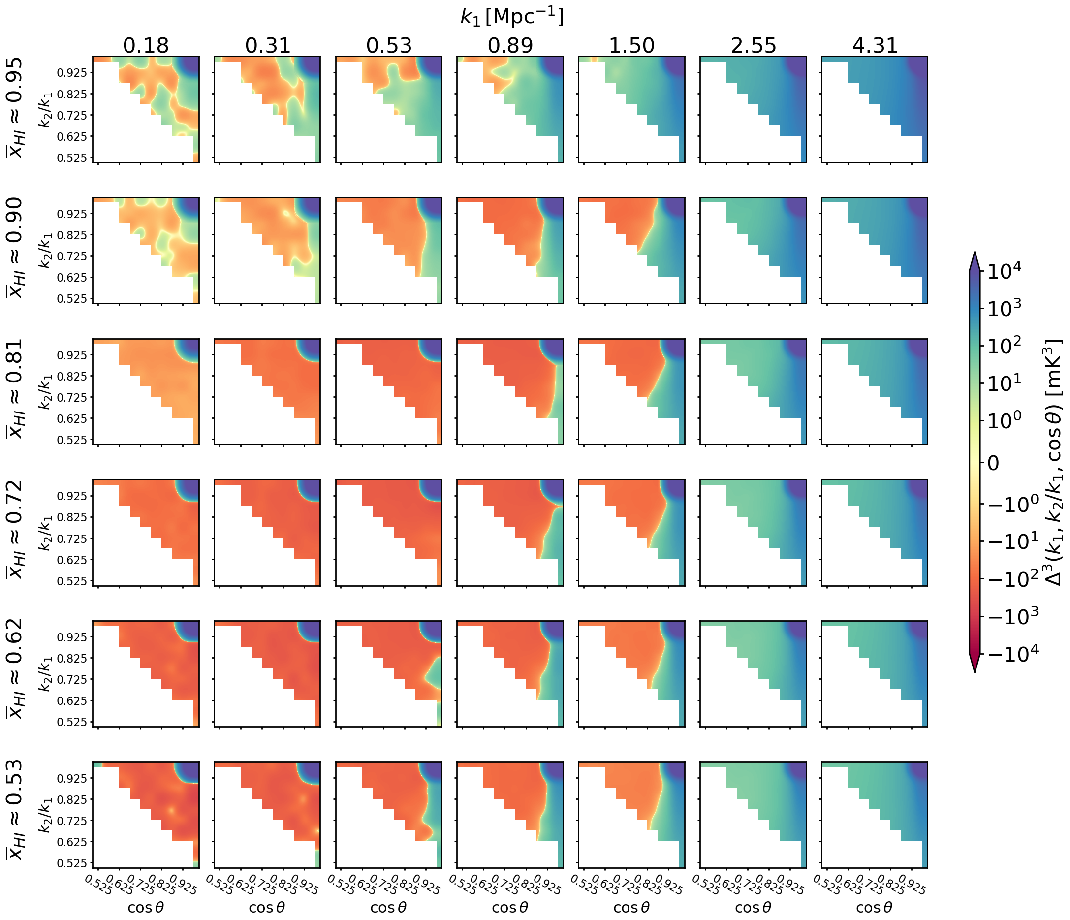
Figure 1: This figure shows the [H i]${}_{\text{21cm}}$ auto-bispectrum for all unique triangle configurations and averaged over all realizations of astrophysical scatter. This is shown for the full set of neutral fraction range that has been considered here.

The results on the impact of scatter on the bispectrum are presented in subsection 5.1. The corresponding statistical significance of our results is shown in subsection 5.2, along with a comparison to the power spectrum statistic in subsection 5.3. Finally, we also present a detectability analysis of the [H i]${}_{\text{21cm}}$ bispectrum which is affected by the astrophysical scatter, in subsection 5.4.

5.1 Impact of scatter on the bispectrum for all unique triangles

We present our results on the impact of scatter on the [H i]${}_{\text{21cm}}$ bispectrum in Figure 2. The labels in Figure 2 are identical to those of Figure 1. The quantity plotted in Figure 2 is |$\langle\Delta B\rangle/B_{\text{no-scatter}}$|. The ratio |$\langle\Delta B\rangle/B_{\text{no-scatter}}$| can be more than a factor of $10$ for some configurations. However, as we explore in the following subsection, this change is not statistically significant and can vary substantially from realizations to realizations for $k_{1}$ modes up to 1.5 Mpc^-1.

At scales $k_{1}\sim$ $2.55$ Mpc^-1, we see that most of the $\cos\theta$ - $k_{2}/k_{1}$ bispectrum configuration space is affected due to the presence of astrophysical scatter. The ratio |$\langle\Delta B\rangle/B_{\text{no-scatter}}$| is $\sim 0.2$ at $\overline{x}_{\text{H\,{i}}}\approx 0.53$. At $\overline{x}_{\text{H\,{i}}}\approx 0.81$, the ratio goes up to $\sim 1$, which then declines again at $\overline{x}_{\text{H\,{i}}}\approx 0.95$. The region of the affected $\cos\theta$ - $k_{2}/k_{1}$ configuration space gradually grows, as we go to higher neutral fractions, and saturation appears at the highest neutral fraction that we consider in our simulated [H i]${}_{\text{21cm}}$ maps.

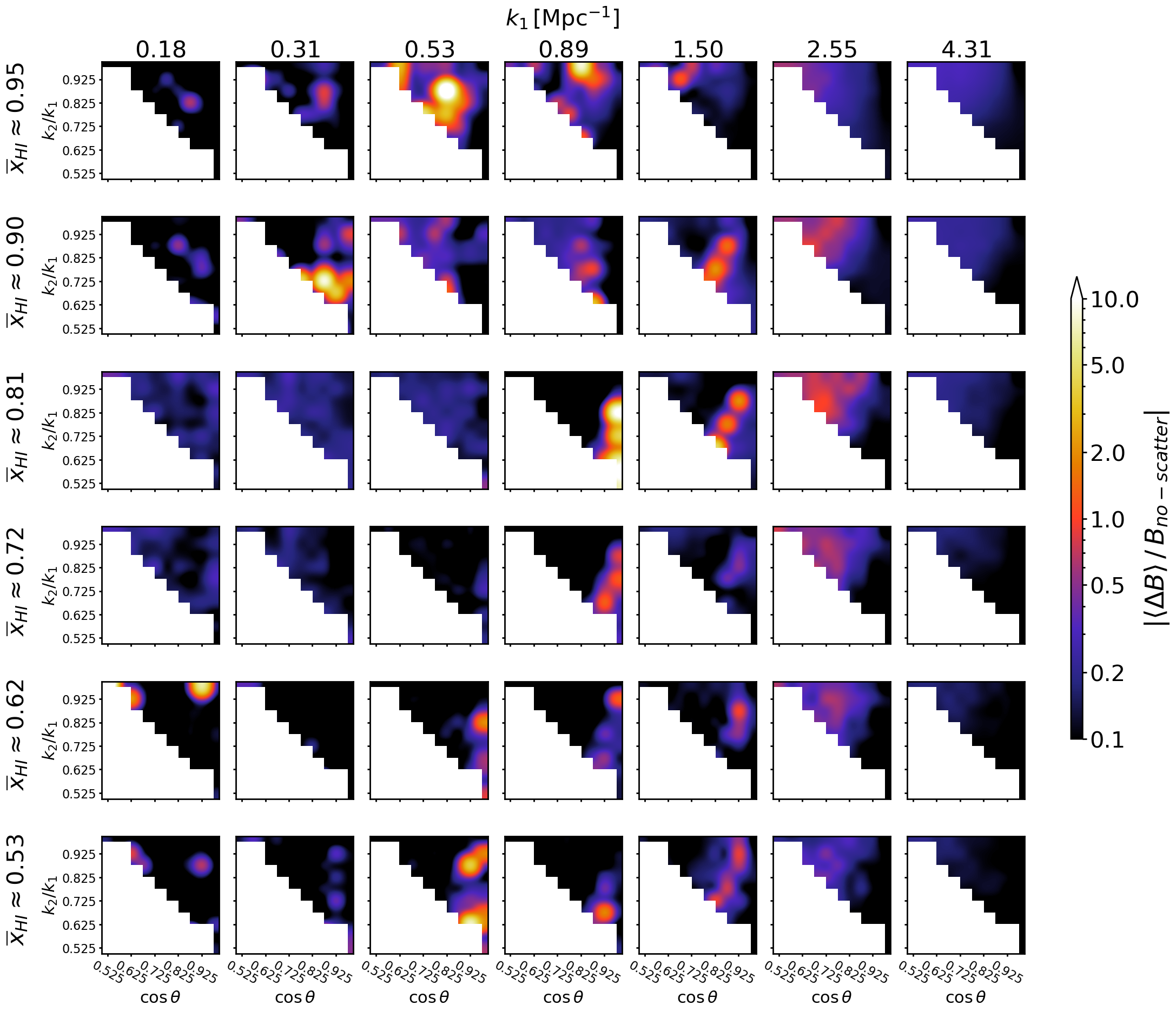
Figure 2: Impact on bispectrum due to the astrophysical scatter is shown here. The rows represent the average neutral fractions for a given averaged realization. The columns represent $k_{1}$ modes for the bispectrum. The color bar scale represent the change ($\langle B\rangle$) compared to the bispectrum for the no-scatter case ($B_{\text{no-scatter}}$).

5.2 Statistical significance

Since the astrophysical scatter is a stochastic phenomenon, any statistic used to study this will have an associated variance arising from the stochasticity. It is thus important to investigate the statistical significance of the impact discussed in previous subsection 5.1 and Figure 2. The realization-to-realization variance is estimated for the bispectrum as $\sigma^{2}_{\Delta B}=\sum_{\text{R}}(\Delta B_{\text{R}}-\langle\Delta B\rangle)^{2}/N$, with $N=50$ being the number of independent realizations of the scatter. We use the quantity $|\langle\Delta B\rangle/\sigma_{\Delta B}|$ to estimate the statistical significance of the impact of scatter.

In Figure 3, we see that at large and intermediate scales up to $k_{1}\lesssim 1$ Mpc^-1 , the impact is not statistically significant ($|\langle\Delta B\rangle/\sigma_{\Delta B}|\sim 1$). At these scales, there are occasional occurrences of $2\sigma$ impact at $\overline{x}_{\text{H\,{i}}}\gtrsim 0.81$. These suggest that effects due to astrophysical scatter on the bispectrum are not significant at large and intermediate scales. However, at $k_{1}\gtrsim$ 2.55 Mpc^-1, we see that the change is significant with more than $3\sigma$ significance at $\overline{x}_{\text{H\,{i}}}\approx 0.53$, for almost all $\cos\theta$ - $k_{2}/k_{1}$ configurations. The significance becomes $>5\sigma$ for $\overline{x}_{\text{H\,{i}}}\gtrsim 0.81$, and further increases for higher neutral fractions.

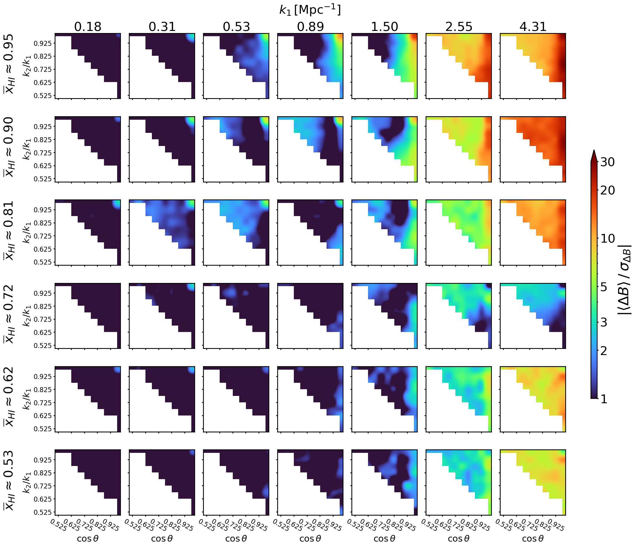
Figure 3: Statistical significance of the impact of scatter on the bispectrum is shown here, with rows representing average neutral fraction $\overline{x}_{\text{H\,{i}}}$ and columns representing $k_{1}$ mode of the bispectrum.

We find that large ionized bubbles remain very similar in different realizations of astrophysical scatter. This can be seen in Figure 4 which shows [H i]${}_{\text{21cm}}$ maps for $10$ different realizations of the scatter, whereas the underlying DM field and halo list are same. We see that the largest ionized bubble in different maps remains largely unaffected. However, the sizes of small ionized bubbles vary considerably in different realizations. This is more clear in Figure 5 which shows a zoomed-in version of a particular region of Figure 4, focusing on a small ionized bubble. Small ionized bubbles encompass a few low-mass DM haloes and the number of ionizing photons emitted by them vary in different realizations due to the scatter. This results in the size of small ionized bubbles to vary considerably across realizations. This is not the case for large bubbles which encompass many more DM haloes and the collective number of ionizing photons does not vary much across realizations. Therefore, the impact of scatter is more prominent in the small ionized bubble size distribution, whereas it is largely negligible in large ionized bubbles. In the absence of large ionized bubbles in a highly neutral medium at the early stages of reionization, the signatures of astrophysical scatter are retained and captured in the auto-bispectrum at the small scales, with high statistical significance. In contrast, the effect is not visible at large scales, at later stages of the EoR.

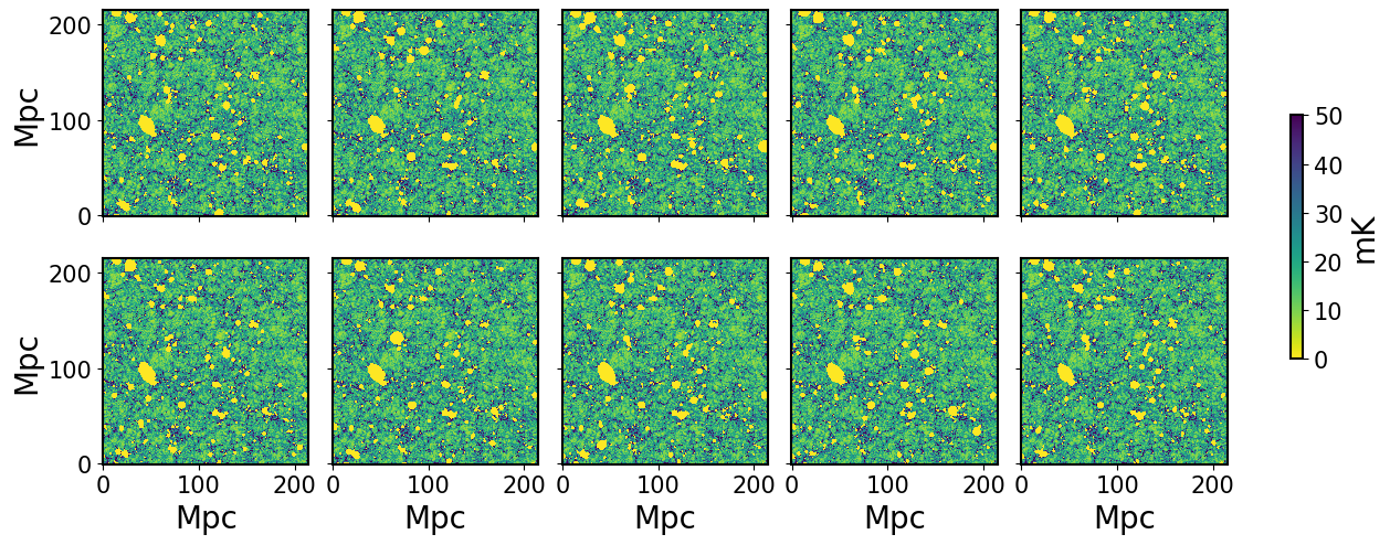
Figure 4: Different scatter realizations of the full $215\,\text{Mpc}\times 215\,\text{Mpc}$ slice is shown at a fixed neutral fraction of $\overline{x}_{\text{H\,{i}}}\approx 0.81$.

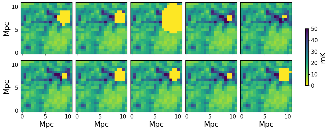
Figure 5: Realization to Realization fluctuation of a particular ionized bubble is shown here on a scale of $\approx 10\,\text{Mpc}\times 10\,\text{Mpc}$ at a fixed neutral fraction of $\overline{x}_{\text{H\,{i}}}\approx 0.81$.

5.3 Comparison with the power spectrum

In this section, we do a similar analysis of the impact of astrophysical scatter on the auto-power spectrum, as is done with auto-bispectrum (as described in previous sections), and compare it with the latter to understand how the auto-bispectrum can capture information that the power spectrum might fail to do. We estimate the auto-power spectrum for the no-scatter scenario and all of the 50 realizations of the scenario with astrophysical scatter. In Figure 6, top panel, we compare the power spectrum for the scatter scenario averaged over all realizations (red-dashed line) with that of the no-scatter case (black-solid line). In the middle panel, we present the percentage change in the auto-power spectrum due to scatter and the corresponding statistical significance of the impact in the bottom panel.

For the neutral fractions, $\overline{x}_{\text{H\,{i}}}=0.53-0.81$, the magnitude of the impact ranges from $5-15$ per cent, with statistical significance ranging from $4\sigma-5\sigma$. At $\overline{x}_{\text{H\,{i}}}=0.90$ and $\overline{x}_{\text{H\,{i}}}=0.95$, the statistical significance is very high ($10\sigma$ and $14\sigma$ respectively), at the peak of the impact of astrophysical scatter. However, it is less ($\sim 10$ per cent and $\sim 5$ per cent respectively) compared to the magnitude of the impact at $\overline{x}_{\text{H\,{i}}}=0.81$. Unlike the auto-bispectrum, the impact on the auto-power spectrum is at a single-length scale, with the maximum impact at $k\sim 0.2$ Mpc^-1 being $\lesssim 15$ per cent for $\overline{x}_{\text{H\,{i}}}=0.81$. The magnitude of the maximum impact declines and shifts to smaller scales for the higher neutral fractions. The magnitude of the maximum impact is broadly consistent with the findings of Hassan et al. (2022). However, they present their results based on the ionization auto-power spectrum (different from the auto-power spectrum of the brightness temperature fluctuations), which does not include a corresponding statistical significance analysis.

On the other hand, the auto-bispectrum, being a 3-pt Fourier statistic, captures the impact of scatter on the correlations between different length scales. This impact consistently exceeds 20 per cent across all neutral fractions ($\overline{x}_{\text{H\,{i}}}$) $\geq 0.53$ at $k\sim 2.55$ Mpc^-1, with statistical significance consistently equal to or higher than $3\sigma$. At $\overline{x}_{\text{H\,{i}}}=0.81$, the impact of astrophysical scatter reaches $\sim 100$ per cent for a significant region of the auto-bispectrum triangle configuration space at $5\sigma$ statistical significance. It suggests that the impact of the astrophysical scatter on the [H i]_21cm signal is captured and characterized in a more detailed manner with the auto-bispectrum as opposed to the auto-power spectrum, which misses out on the signatures of the impact of scatter at the relevant neutral fractions and length-scales, with sufficient magnitude.

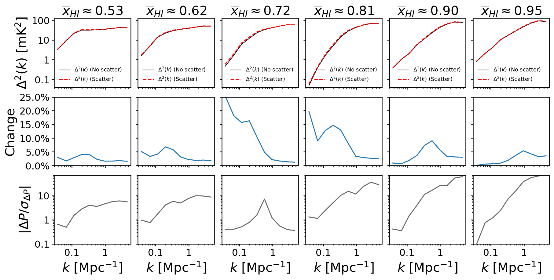
Figure 6: Impact on the power spectrum due to the astrophysical scatter is shown here, along with the statistical significance.

5.4 Detectability of the [H I] 21cm auto-bispectrum

Here, we explore the possibility of detecting the impact of the scatter on the [H i]${}_{\text{21cm}}$ bispectrum considering SKA1-Low observations. We compute the variance in the bispectrum ($\sigma^{2}_{\rm N}(B)$) due to system noise using (Scoccimarro et al., 2004; Liguori et al., 2010):

$$\sigma^{2}_{\text{N}}(B)\approx s_{B}\frac{V_{f}}{V_{B}}P_{\text{N}}(k_{1},z)P_{\text{N}}(k_{2},z)P_{\text{N}}(k_{3},z)$$ (4)

Here, $V_{f}=(2\pi)^{3}/V_{\text{s}}$ is the volume of the fundamental cell in the Fourier domain, with $V_{s}$ being the survey volume, and $P_{\rm N}(k,z)$ is the noise power spectrum contributed by the system noise. As a test case, we limit our analysis to only equilateral triangle configurations of the bispectrum, which are expected to be affected the most by the system noise. In equation 4, $s_{B}$ = 6 for equilateral triangles, and $V_{B}\approx 8\pi^{2}k_{1}k_{2}k_{3}\Delta k_{1}\Delta k_{2}\Delta k_{3}$. The noise power spectrum due to the system noise in radio interferometric experiment is given by (Bull et al., 2015; Obuljen et al., 2018):

$$P_{\text{N}}(k,z)=\frac{T^{2}_{\text{sys}}(z)\chi^{2}(z)r_{\nu}(z)\lambda^{4}(z)}{A^{2}_{\text{eff}}t_{\text{obs}}n_{\text{pol}}n(\bm{u},z)\nu_{\text{21cm}}}.$$ (5)

$\chi(z)$ is the comoving distance to redshift $z$, and $r_{\nu}=(c/H(z))(1+z)^{2}$. $\lambda(z)=21\times(1+z)$ cm and $\nu_{\text{21cm}}=1420\,\text{MHz}$, are the redshifted wavelength and the rest frame frequency of the [H i]${}_{\text{21cm}}$ emission, respectively. We assume the number of polarization ($n_{\text{pol}}$) to be $2$ and $n(\bm{u},z)=N^{2}_{\text{a}}/(2\pi u^{2}_{\text{max}})$ is the baseline density which we assume to be constant within the core radius. $N_{\text{a}}$ is the total number of antennae in the experiment and $u_{\text{max}}$ is the maximum baseline in units of $\lambda(z)$. The system temperature $T_{\text{sys}}$ is modeled as $T_{\text{sys}}(\nu)=100\,+\,300(150\,\text{MHz}/\nu)^{2.55}\,\text{K}$ following Mellema et al. (2013). $A_{\text{eff}}$ is the effective collecting area of each antenna which is modeled as, $A_{\text{eff}}=A_{\text{eff}}(\nu_{\text{crit}})\times\epsilon(\nu)$ (Bull et al., 2015), where $\epsilon(\nu)$ is defined as

$$\epsilon(\nu)=\bigg{\{}\begin{tabular}[]{lr}$(\nu_{\text{crit}}/\nu)^{2}$,&$\nu>\nu_{\text{crit}}$\\ 1,&$\nu\leq\nu_{\text{crit}}$.\\ \end{tabular}$$ (6)

$A_{\text{eff}}(\nu_{\text{crit}})$ is taken to be 962 m² at $\nu_{\text{crit}}=110$ MHz (Giri et al., 2018). We take $N_{\text{a}}=296$ within a core radius of $R_{\text{max}}=2\,\text{Km}$. The relative $k$-bin size is taken as $\Delta k/k\sim 1$. We assume a test-case scenario where we observe for $t_{\text{obs}}=1000$ hours for a single pointing, assuming a bandwidth of $16$ MHz, and estimate the detectability of the equilateral bispectrum for the signal model considered here.

In Figure 7 we show the dimensionless [H i]${}_{\text{21cm}}$ bispectrum $\Delta^{3}(k_{1},k_{2}/k_{1},\cos\theta)=k^{3}_{1}k^{3}_{2}B(k_{1},k_{2}/k_{1},\cos\theta)/(2\pi^{2})^{2}$ for equilateral triangle configurations. Different colors represent different neutral fractions at redshift $z=7.4$.

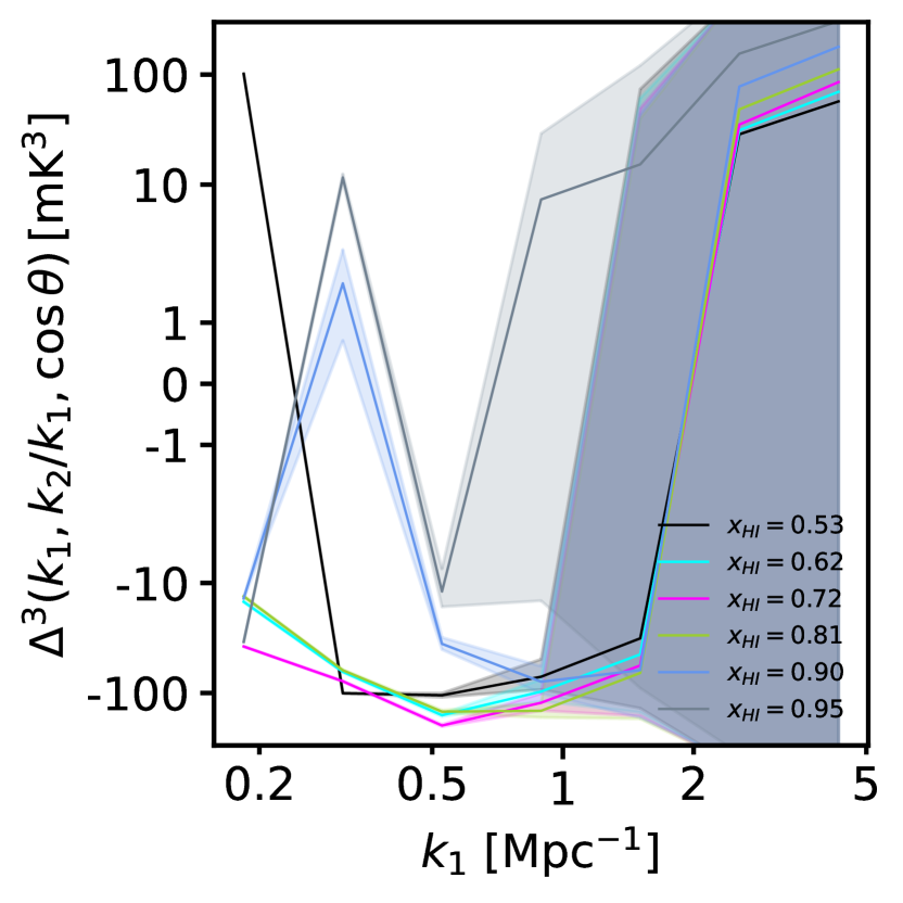
Figure 7: The equilateral bispectrum at $z=7.4$ is plotted for all the neutral fractions, with the shaded regions representing the 1$\sigma$ confidence interval considering instrumental noise.

The shaded regions around each bispectrum plot show the $1\sigma$ uncertainty arising from the system noise. In Figure 8 we show the resulting signal-to-noise ratio (SNR) for $1000$ hours of observations with the SKA1-Low.

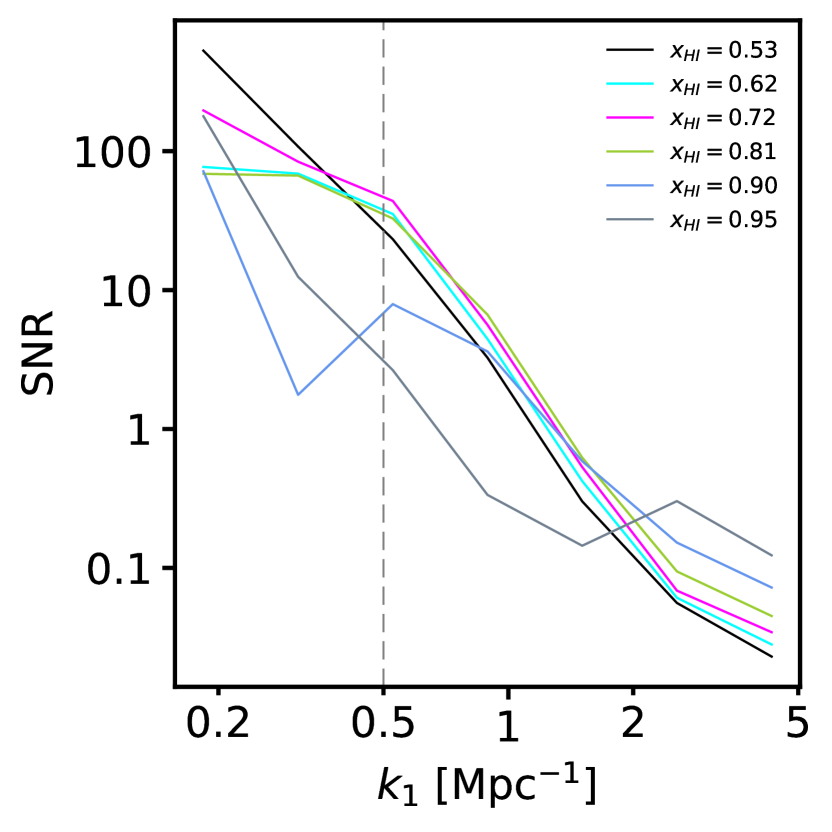
Figure 8: The signal-to-noise ratio (SNR) for the equilateral bispectrum arising only from the instrumental noise at $z=7.4$ for multiple neutral fractions is shown for $t_{\text{obs}}=1000$ hours. The dashed-grey vertical line represents the $k$-mode ($\sim 0.5$ Mpc^-1) below which cosmic variance dominates.

We see that small scales (at $k\gtrsim 1$ Mpc^-1) where the astrophysical scatter has a significant impact on the bispectra are completely dominated by the system noise. Therefore, it is very unlikely that the SKA1-Low like experiments will be able to detect the impact of the astrophysical scatter on [H i]${}_{\text{21cm}}$ bispectra during the EoR. However, we point out that the formalism for the noise estimation presented here is approximate and predictions may change to some extent if one uses a complete numerical approach (Mondal et al., 2021). Further, this study has not considered the uncertainty in bispectrum measurements arising from cosmic variance, which will mainly dominate at large scales. The vertical dashed line in Figure 8 indicates the $k$-mode below which the cosmic variance dominates, as estimated by Mondal et al. (2021).

6 Summary and Discussion

The [H i]${}_{\text{21cm}}$ signal is a promising probe of the Universe during the EoR and can be used to track the evolution of the early IGM and the reionization process. Although the power spectrum can shed light on many important issues, it can not capture the entire information content in the [H i]${}_{\text{21cm}}$ signal as it is highly non-Gaussian. The Bispectra can capture some aspects of non-Gaussian [H i]${}_{\text{21cm}}$ signal. The variability in the ionizing photon emission rates from one halo to another also referred to as astrophysical scatter, can introduce an additional non-Gaussianity into the signal. In this work, we study the impact of the astrophysical scatter on the [H i]${}_{\text{21cm}}$ bispectra during the EoR. We simulated [H i]${}_{\text{21cm}}$ maps using a semi-numerical prescription that also incorporates astrophysical scatter. We estimate the fractional change in the bispectra $|\Delta B/B_{\text{no-scatter}}|$ due to the scatter. We also study the statistical significance of the change by estimating the quantity $|\Delta B/\sigma_{\Delta B}|$, where $\sigma^{2}_{\Delta B}$, which is the variance in the $\Delta B$, has been estimated using $50$ independent realizations of the scatter. Here, the analysis is presented for all unique triangle configurations of the bispectrum, for a range of neutral fractions, at a fixed redshift of $z=7.4$. We find that:

• The large and intermediate scales ($k_{1}\lesssim 1.5$ Mpc^-1) are largely unaffected due to astrophysical scatter. Although, the quantity $|\Delta B/B_{\text{no-scatter}}|$ is more than a factor of $\sim 10$ in some regions of the bispectrum configuration space for these length scales, this impact is found to be non-significant.

• We see a significant impact at scales $k_{1}\gtrsim 2.55$ Mpc^-1, where $|\Delta B/B_{\text{no-scatter}}|\gtrsim 20$ per cent for all neutral fractions explored in this study. The fractional change in bispectra due to the scatter can be as high as $\sim 100$ per cent for high enough neutral fractions ($\overline{x}_{\text{H\,{i}}}\sim 0.81$).

• The presence of astrophysical scatter primarily affects the small ionized regions surrounded by a highly neutral background. On the other hand, large ionized bubbles would be formed as a result of ionization from the cumulative photon counts from multiple sources, thus averaging out the signatures of astrophysical scatter, as similarly argued in Hassan et al. (2022). Therefore large-length scales would be primarily unaffected by the presence of scatter in the number distribution of the ionizing photons.

• We present a detectability analysis for our bispectrum signal following Scoccimarro et al. (2004); Liguori et al. (2010) and considering the equilateral bispectrum triangle configuration. We find that the SKA1-Low like experiments may not have enough sensitivity to detect the small-scale signatures of the scatter on bispectra. Large-scale bispectra will remain undetected due to the dominance of the cosmic variance.

We would like to point out that the entire study was performed considering only one value of the $\sigma$ (defined in equation 3). The impact of the scatter on the IGM [H i]_21cm signal may vary with different values of $\sigma$. One would require to generate a large number of statistically independent realizations of [H i]_21cm signal with different values of $\sigma$ in order to perform a detailed study of the impact. We defer this for future work.

Further, there are a few more limitations in our study. We do not explicitly estimate the cosmic variance error in the bispectrum which will affect the large scales. Throughout our study, we have assumed that the spin temperature ($T_{\text{s}}$) is much higher than the cosmic microwave background radiation temperature ($T_{\gamma}$). This may not be true during the early stages of the EoR. This assumption will affect the $\delta T_{\text{b}}$ fluctuations since $\delta T_{\text{b}}(\bm{x},z)\propto(1-T_{\gamma}(z)/T_{\text{s}}(\bm{x},z))$ (Bharadwaj & Ali, 2005), and Lyman-$\alpha$ coupling and heating of the IGM will play a role in determining these fluctuations. This study assumes that star-forming galaxies drive the entire cosmic reionization process. We have not considered contributions from other sources, such as uniform ionizing background (UIB) originating from active galactic nuclei or X-ray radiation from X-ray binaries or mini-QSOs (McQuinn, 2012; Mesinger et al., 2013; Majumdar et al., 2016). Here, we also have not modelled the inhomogenous recombination process of the ionized hydrogen, which would affect the ionization morphology of the Universe. It might affect how the astrophysical scatter of the star-forming galaxies affects the reionization process under this cumulative scenario of all possible sources of ionizing photons, contributing to the reionization processes.

The auto-bispectrum is a valuable statistic for capturing various non-Gaussian information from the [H i]${}_{21\text{cm}}$ signal. Our study finds that this higher-order Fourier statistic is statistically unaffected by the astrophysical scatter at length scales which are practically detectable by the current generation of radio interferometers and upcoming ones in the near future, such as SKA1-Low. Therefore, models of cosmic reionization, which do not consider the astrophysical scatter of star-forming galaxies, serve as a viable approach for modelling the [H i]${}_{21\text{cm}}$ signal. However, any futuristic next-generation radio interferometer setup with improved sensitivity might be able to probe the relevant length scales where the contributions of the astrophysical scatter to the [H i]${}_{21\text{cm}}$ signal non-Gaussianities are significant.

Data Availability

The simulated data underlying this work will be shared upon reasonable request to the corresponding author.

References

- Astropy Collaboration et al. (2022) Astropy Collaboration et al., 2022, ApJ, 935, 167
- Bharadwaj & Ali (2005) Bharadwaj S., Ali S. S., 2005, MNRAS, 356, 1519
- Bharadwaj & Pandey (2005) Bharadwaj S., Pandey S. K., 2005, MNRAS, 358, 968
- Bharadwaj & Srikant (2004) Bharadwaj S., Srikant P. S., 2004, Journal of Astrophysics and Astronomy, 25, 67
- Bharadwaj et al. (2020) Bharadwaj S., Mazumdar A., Sarkar D., 2020, MNRAS, 493, 594
- Blank et al. (2021) Blank M., Meier L. E., Macciò A. V., Dutton A. A., Dixon K. L., Soliman N. H., Kang X., 2021, MNRAS, 500, 1414
- Breysse et al. (2014) Breysse P. C., Kovetz E. D., Kamionkowski M., 2014, MNRAS, 443, 3506
- Bull et al. (2015) Bull P., Ferreira P. G., Patel P., Santos M. G., 2015, ApJ, 803, 21
- Choudhury & Paranjape (2018) Choudhury T. R., Paranjape A., 2018, MNRAS, 481, 3821
- Choudhury et al. (2009) Choudhury T. R., Haehnelt M. G., Regan J., 2009, Monthly Notices of the Royal Astronomical Society, 394, 960
- Daddi et al. (2007) Daddi E., et al., 2007, ApJ, 670, 156
- Datta et al. (2012) Datta K. K., Mellema G., Mao Y., Iliev I. T., Shapiro P. R., Ahn K., 2012, MNRAS, 424, 1877
- Dutton et al. (2010) Dutton A. A., van den Bosch F. C., Dekel A., 2010, MNRAS, 405, 1690
- Field (1958) Field G. B., 1958, Proceedings of the IRE, 46, 240
- Furlanetto et al. (2004) Furlanetto S. R., Zaldarriaga M., Hernquist L., 2004, ApJ, 613, 1
- Gill et al. (2023) Gill S. S., Pramanick S., Bharadwaj S., Shaw A. K., Majumdar S., 2023, Submitted in MNRAS
- Giri et al. (2018) Giri S. K., Mellema G., Ghara R., 2018, MNRAS, 479, 5596
- Gong et al. (2011) Gong Y., Cooray A., Silva M. B., Santos M. G., Lubin P., 2011, ApJ, 728, L46
- Gong et al. (2012) Gong Y., Cooray A., Silva M., Santos M. G., Bock J., Bradford C. M., Zemcov M., 2012, ApJ, 745, 49
- Harker et al. (2009) Harker G. J. A., et al., 2009, MNRAS, 393, 1449
- Harris et al. (2020) Harris C. R., et al., 2020, Nature, 585, 357
- Hassan et al. (2022) Hassan S., Davé R., McQuinn M., Somerville R. S., Keating L. C., Anglés-Alcázar D., Villaescusa-Navarro F., Spergel D. N., 2022, ApJ, 931, 62
- Hutter et al. (2020) Hutter A., Watkinson C. A., Seiler J., Dayal P., Sinha M., Croton D. J., 2020, MNRAS, 492, 653
- Iliev et al. (2006) Iliev I. T., Mellema G., Pen U. L., Merz H., Shapiro P. R., Alvarez M. A., 2006, MNRAS, 369, 1625
- Kamran et al. (2021) Kamran M., Ghara R., Majumdar S., Mondal R., Mellema G., Bharadwaj S., Pritchard J. R., Iliev I. T., 2021, MNRAS, 502, 3800
- Karoumpis et al. (2022) Karoumpis C., Magnelli B., Romano-Díaz E., Haslbauer M., Bertoldi F., 2022, A&A, 659, A12
- Kubota et al. (2016) Kubota K., Yoshiura S., Shimabukuro H., Takahashi K., 2016, PASJ, 68, 61
- Lagos et al. (2018) Lagos C. d. P., Tobar R. J., Robotham A. S. G., Obreschkow D., Mitchell P. D., Power C., Elahi P. J., 2018, MNRAS, 481, 3573
- Li et al. (2016) Li T. Y., Wechsler R. H., Devaraj K., Church S. E., 2016, ApJ, 817, 169
- Lidz et al. (2011) Lidz A., Furlanetto S. R., Oh S. P., Aguirre J., Chang T.-C., Doré O., Pritchard J. R., 2011, ApJ, 741, 70
- Liguori et al. (2010) Liguori M., Sefusatti E., Fergusson J. R., Shellard E. P. S., 2010, Advances in Astronomy, 2010, 980523
- Madau et al. (1997) Madau P., Meiksin A., Rees M. J., 1997, ApJ, 475, 429
- Magdis et al. (2010) Magdis G. E., Rigopoulou D., Huang J.-S., Fazio G. G., 2010, MNRAS, 401, 1521
- Majumdar et al. (2014) Majumdar S., Mellema G., Datta K. K., Jensen H., Choudhury T. R., Bharadwaj S., Friedrich M. M., 2014, Monthly Notices of the Royal Astronomical Society, 443, 2843
- Majumdar et al. (2016) Majumdar S., et al., 2016, MNRAS, 456, 2080
- Majumdar et al. (2018) Majumdar S., Pritchard J. R., Mondal R., Watkinson C. A., Bharadwaj S., Mellema G., 2018, MNRAS, 476, 4007
- Majumdar et al. (2020) Majumdar S., Kamran M., Pritchard J. R., Mondal R., Mazumdar A., Bharadwaj S., Mellema G., 2020, MNRAS, 499, 5090
- Mas-Ribas & Chang (2020) Mas-Ribas L., Chang T.-C., 2020, Phys. Rev. D, 101, 083032
- Matthee & Schaye (2019) Matthee J., Schaye J., 2019, MNRAS, 484, 915
- McQuinn (2012) McQuinn M., 2012, MNRAS, 426, 1349
- Mellema et al. (2006) Mellema G., Iliev I. T., Pen U.-L., Shapiro P. R., 2006, MNRAS, 372, 679
- Mellema et al. (2013) Mellema G., et al., 2013, Experimental Astronomy, 36, 235
- Mellema et al. (2015) Mellema G., Koopmans L., Shukla H., Datta K. K., Mesinger A., Majumdar S., 2015, in Proceedings of Advancing Astrophysics with the Square Kilometre Array — PoS(AASKA14). p. 010, doi:10.22323/1.215.0010
- Mesinger et al. (2013) Mesinger A., Ferrara A., Spiegel D. S., 2013, MNRAS, 431, 621
- Mondal et al. (2015) Mondal R., Bharadwaj S., Majumdar S., Bera A., Acharyya A., 2015, Monthly Notices of the Royal Astronomical Society: Letters, 449, L41
- Mondal et al. (2017) Mondal R., Bharadwaj S., Majumdar S., 2017, MNRAS, 464, 2992
- Mondal et al. (2021) Mondal R., Mellema G., Shaw A. K., Kamran M., Majumdar S., 2021, MNRAS, 508, 3848
- Moradinezhad Dizgah et al. (2022) Moradinezhad Dizgah A., Nikakhtar F., Keating G. K., Castorina E., 2022, J. Cosmology Astropart. Phys., 2022, 026
- Moradinezhad Dizgah et al. (2023) Moradinezhad Dizgah A., Bellini E., Keating G. K., 2023, arXiv e-prints, p. arXiv:2304.08471
- Murmu et al. (2021) Murmu C. S., Majumdar S., Datta K. K., 2021, MNRAS, 507, 2500
- Murmu et al. (2022) Murmu C. S., Ghara R., Majumdar S., Datta K. K., 2022, arXiv e-prints, p. arXiv:2210.09612
- Murmu et al. (2023) Murmu C. S., et al., 2023, MNRAS, 518, 3074
- Noeske et al. (2007) Noeske K. G., et al., 2007, ApJ, 660, L43
- Obuljen et al. (2018) Obuljen A., Castorina E., Villaescusa-Navarro F., Viel M., 2018, J. Cosmology Astropart. Phys., 2018, 004
- Padmanabhan (2019) Padmanabhan H., 2019, MNRAS, 488, 3014
- Padmanabhan (2023) Padmanabhan H., 2023, MNRAS, 523, 3503
- Peng & Maiolino (2014) Peng Y.-j., Maiolino R., 2014, MNRAS, 443, 3643
- Peterson & Suarez (2012) Peterson J. B., Suarez E., 2012, arXiv e-prints, p. arXiv:1206.0143
- Planck Collaboration et al. (2014) Planck Collaboration et al., 2014, A&A, 571, A16
- Pullen et al. (2014) Pullen A. R., Doré O., Bock J., 2014, ApJ, 786, 111
- Raste et al. (2023) Raste J., Kulkarni G., Watkinson C. A., Keating L. C., Haehnelt M. G., 2023, arXiv e-prints, p. arXiv:2308.09744
- Ross et al. (2021) Ross H. E., Giri S. K., Mellema G., Dixon K. L., Ghara R., Iliev I. T., 2021, MNRAS, 506, 3717
- Roy et al. (2023) Roy A., Valentín-Martínez D., Wang K., Battaglia N., van Engelen A., 2023, arXiv e-prints, p. arXiv:2304.06748
- Schaan & White (2021) Schaan E., White M., 2021, J. Cosmology Astropart. Phys., 2021, 068
- Scoccimarro et al. (2004) Scoccimarro R., Sefusatti E., Zaldarriaga M., 2004, Phys. Rev. D, 69, 103513
- Shimabukuro et al. (2015) Shimabukuro H., Yoshiura S., Takahashi K., Yokoyama S., Ichiki K., 2015, MNRAS, 451, 467
- Silva et al. (2013) Silva M. B., Santos M. G., Gong Y., Cooray A., Bock J., 2013, The Astrophysical Journal, 763, 132
- Silva et al. (2015) Silva M., Santos M. G., Cooray A., Gong Y., 2015, ApJ, 806, 209
- Speagle et al. (2014) Speagle J. S., Steinhardt C. L., Capak P. L., Silverman J. D., 2014, ApJS, 214, 15
- Watkinson & Pritchard (2014) Watkinson C. A., Pritchard J. R., 2014, MNRAS, 443, 3090
- Watkinson & Pritchard (2015) Watkinson C. A., Pritchard J. R., 2015, MNRAS, 454, 1416
- Whitaker et al. (2012) Whitaker K. E., van Dokkum P. G., Brammer G., Franx M., 2012, ApJ, 754, L29
- Wouthuysen (1952) Wouthuysen S. A., 1952, AJ, 57, 31
- Yang et al. (2022) Yang S., Popping G., Somerville R. S., Pullen A. R., Breysse P. C., Maniyar A. S., 2022, ApJ, 929, 140
- Yue & Ferrara (2019) Yue B., Ferrara A., 2019, MNRAS, 490, 1928
- Zawada et al. (2014) Zawada K., Semelin B., Vonlanthen P., Baek S., Revaz Y., 2014, MNRAS, 439, 1615