Material Palette: Extraction of Materials from a Single Image

Abstract

In this paper, we propose a method to extract Physically-Based-Rendering (PBR) materials from a single real-world image. We do so in two steps: first, we map regions of the image to material concepts using a diffusion model, which allows the sampling of texture images resembling each material in the scene. Second, we benefit from a separate network to decompose the generated textures into Spatially Varying BRDFs (SVBRDFs), providing us with materials ready to be used in rendering applications. Our approach builds on existing synthetic material libraries with SVBRDF ground truth, but also exploits a diffusion-generated RGB texture dataset to allow generalization to new samples using unsupervised domain adaptation (UDA). Our contributions are thoroughly evaluated on synthetic and real-world datasets. We further demonstrate the applicability of our method for editing 3D scenes with materials estimated from real photographs. The code and models will be made open-source.

1 Introduction

Whether it is a soft blanket, a rugged carpet, or a crumbling stone, humans can identify materials from a photograph. Besides geometry understanding, this ability derives from our sensing of how light interacts with materials, allowing us to identify the substance at stake without even touching it. In sciences, this has pushed research in spectrophotometry [18] or light sensing [4], while in the arts, Vermeers and Caravaggio among others have used this long standing observation to convey the feeling of materials in their paintings. Modern CG artists also deploy significant efforts to mimic realistic light-material interaction, through the design of Physically-Based Rendering materials (PBR). While many libraries of material assets exist, no dataset can capture the true variety of real-world materials. What is more, capturing real-world materials is still a complex endeavor requiring special apparatus [2]. In many scenarios, however, one may wish to estimate a material from a single RGB image, for example, to capture a unique marble stone in a visit or the fur of a wild animal from a souvenir photo.

Hence, we formulate the novel task of extracting PBR materials from a single real-world image, as shown in Fig. 1. Given a set of regions, our method solves this task by generating corresponding textures along with their Spatially Varying BRDFs (SVBRDFs) without a priori knowledge about the capturing viewpoint, scene geometry or lighting. This sets our work aside from the literature. We coined our method $\color[rgb]{0.09,0.45,0.27}\mathsf{Material~{}Palette}$ because, just like a painter would create their own color mix, one can create their palette of materials from their own photos (Fig. 1, left and right). Moreover, extracted materials are readily usable for CG applications such as 3D renderings (Fig. 1, middle).

There are major challenges in the estimation of PBR materials from just one RGB image, since single-view decomposition is highly ill-posed [9]. To address these hurdles, we rely on recent advances in text-to-image generation [46, 38, 44] to disentangle the specific material appearance from the scene geometry and imaging conditions, allowing us to generate close-up tileable RGB textures of the materials in the scene. We further extract the PBR intrinsics of these diffusion-generated images, with a domain adaptation strategy that benefits from a novel synthetic dataset. Experiments show that $\color[rgb]{0.09,0.45,0.27}\mathsf{Material~{}Palette}$ outputs convincing results and performs better than baselines. The extracted materials closely resemble their real-world counterparts, which makes them usable for 3D scene editing.

We contribute in the following ways:

• We formulate the novel challenging task of material extraction from a single real-world image.

• We propose ‘$\color[rgb]{0.09,0.45,0.27}\mathsf{Material~{}Palette}$’, a method to extract materials within an image, operating in either a user-assisted or fully automated mode (Sec. 3.4).

• Given an image region, we show how a finetuned text-to-image diffusion model can generate realistic tileable texture images (Sec. 3.2) suitable for SVBRDF estimation (Sec. 3.3).

• We provide a non-trivial evaluation pipeline to assess the quality of extracted PBR materials along with a novel prompt-generated dataset named TexSD. Experiments show our materials are close to those of real material datasets and readily usable for 3D editing.

2 Related works

To the best of our knowledge, we are the first to address end-to-end extraction of multiple materials from single real-world images but we cover literature connected to our task.

Single-image intrinsics decomposition.

Long after the pioneering work of [21], deep networks were leveraged for decomposition, exploiting their great pixel-wise estimation capabilities. Most early works focused on object-centric scenes with Lambertian assumption [54], user interaction [32], or scene layers [23]. To decompose in-the-wild objects, symmetry [59] or cross-instance [36] constraints are applied, while [24] requires the 3D mesh [24]. Holistic scene decomposition was addressed splitting albedo and shading [3, 37, 29] also with the support of image-to-image translation [33], or inverse rendering [52]. To account for spatially-varying lighting, some use mixture of illuminations or SVBRDF [3, 65, 16, 30, 31]. Notably, many of these works rely on estimated light sources and are designed for either indoor or outdoor scenes. Additionally, they capture the intrinsics of a scene image without distinguishing between the materials present. We instead wish to extract the intrinsics of dominant materials.

Material and texture extraction.

Typical material capture requires expensive multi-view [2] or polarized [11] apparatus. Many use synthetic data to train single-view SVBRDF estimation networks [9], often coupled with additional single-view data [15, 35] or custom training strategies [27, 55, 10]. Importantly, all works mentioned require orthogonal close-up views of the materials which is impractical for real scenes. UMat [45] uses a single image acquired with a flatbed scanner. Closest to our work is PhotoScene [62], but it requires CAD inputs and is limited to a set of synthetic material graphs. Instead, we propose a single-image method targeting real-world material. TexSynth [12] provides a guided texture editing method but does not model explicitly the material.
A connected field is texture extraction from real-world images. Note that while materials model light interaction, textures only describe the spatial arrangement of colors. A common strategy is to cluster the image textures and extend them to full resolution [48, 28] or apply dataset distillation [7]. While we inspire from texture extraction methods, our task differs drastically as we seek to estimate the full SVBRDF – not only the color.

Text-to-image generative models.

Seminal works for text-to-image generations exploited conditional generative networks, allowing generation in constrained scenarios only [63, 61, 66]. Instead, training on billions of samples has been proven effective in generalizing on a wide range of prompts [43, 44]. To this extent, diffusion models are exploited for their stability at scale [44, 38, 50, 46], although adversarial-based methods are also used [51]. MatFuse [57] and ControlMat [56] recently adopted diffusion processes for material generation. We get inspiration from them while avoiding long training times.

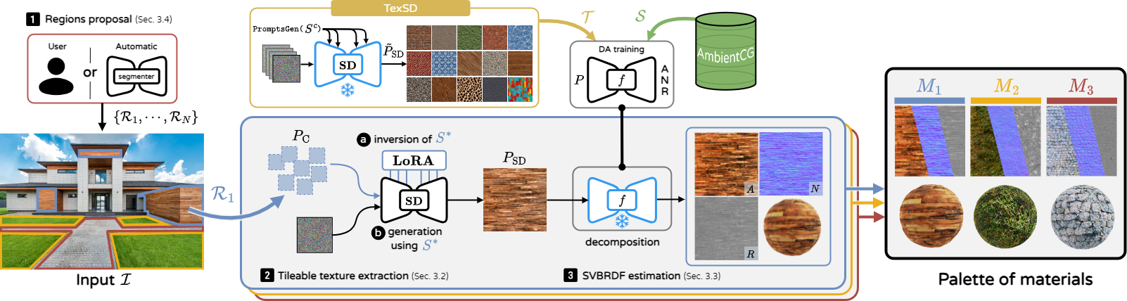
Figure 2: $\boldsymbol{\color[rgb]{0.09,0.45,0.27}\mathsf{Material~{}Palette}}$ pipeline. From a single image $\mathbf{\mathcal{I}}$ (left) our method extracts the SVBRDF of dominant materials (right). Considering a set of regions $\{\mathbf{\mathcal{R}}_{1},\cdots,\mathbf{\mathcal{R}}_{N}\}$ from a user or a segmenter   (Sec. 3.4), we process each region $\mathbf{\mathcal{R}}_{i}$ separately following two steps. In  (Sec. 3.2), we finetune Stable Diffusion [46] on crops of the region $P_{\text{C}}$ to learn a concept $S^{*}$, which is later used to generate a texture image $P_{\text{SD}}$ resembling $P_{\text{C}}$. Then in   (Sec. 3.3), these patches are decomposed into SVBRDF intrinsics maps (Albedo, Normal, Roughness) using a multi-task network. Finally, the output is the palette of extracted materials $\{M_{1},\cdots,M_{N}\}$ corresponding to input regions.

3 Material Palette

Our method extracts Physics-Based Rendering (PBR) materials from regions of a real-world image. Differently from approaches relying on close-up captures [9, 35] or dedicated hardware [2], the problem is much more challenging when given an in-the-wild image (Sec. 3.1) with unknown scene lighting and geometry. Hence, we build on recent advances in vision-language models.

Given an input image $\mathbf{\mathcal{I}}$ and some input regions $\{\mathbf{\mathcal{R}}_{1},\cdots,\mathbf{\mathcal{R}}_{N}\}$, $\color[rgb]{0.09,0.45,0.27}\mathsf{Material~{}Palette}$ extracts a set of corresponding materials SVBRDF $\{M_{1},\cdots,M_{N}\}$. Fig. 2 illustrates the complete pipeline. For each region, we extract a texture approximating its material appearance using Stable Diffusion [46] (Sec. 3.2) . Then, we rely on a domain-adaptive Spatially Varying BRDF (SVBRDF) decomposition using our diffusion prompt-generated samples for generalizing to the extracted textures   (Sec. 3.3). While our pipeline can rely on user input to define the image regions, we can also query any off-the-shelf segmenter   (Sec. 3.4).

3.1 Problem statement

	Multi view training			Single view training
Image	A	N	R	A	N	R

Figure 3: Decomposition with known illumination. Training on ACG [1] we note that even with known lighting, single-view leads to degenerated intrinsics (A,N,R) due to viewpoint ambiguities.

Considering a typical intrinsics decomposition, an image $P$ with known illumination can be approximated as the result of a rendering operation $\tilde{\rho}(.)$ from SVBRDF maps $\tilde{M}=\{\tilde{A},\tilde{N},\tilde{R}\}$, being pixel-wise Albedo, Normals, and Roughness, respectively. This writes: $P=\tilde{\rho}(\tilde{M})$. Our goal is to learn the inverse rendering process with a neural network $f$ to predict $\tilde{M}$ from $P$. In details:

$$f(P)=M=\{A,N,R\}\cong\tilde{M},$$ (1)

where $\tilde{M}$ is the ground truth SVBRDF. A dataset with such labels is obtainable with expensive procedural generation of top-view materials or acquisitions in controlled scenarios [1]. We can train $f$, by rendering multiple views with known illuminations $\tilde{\rho}_{1\dots n}$, and enforcing both a regression loss $\mathcal{L}_{\text{reg}}$ towards the ground truth maps and a multi-view rendering loss $\mathcal{L}_{\text{ren}}$ on the $n$ renderings [19]:

$$\mathcal{L}_{\text{reg}}{=}||M-\tilde{M}||_{1},\,\,\,\,\,\,\mathcal{L}_{\text{ren}}{=}\sum_{i=1}^{n}||\tilde{\rho}_{i}(M)-\tilde{\rho}_{i}(\tilde{M})||_{1}\,.$$ (2)

After training, $f$ can be used to estimate $M$ from unseen images with unknown SVBRDF (Fig. 3, multi-view). However, in our scenario we wish to estimate $M$ from specific regions of an in-the-wild image with variable illumination and geometry, thus being shifted w.r.t. the training distribution of materials datasets. Besides, even assuming known illumination a single view is ambiguous for surface normals and roughness estimation (Fig. 3, single-view).

Without any geometry or illumination priors, we tackle the problem per region by extracting tileable textures which are then decomposed into SVBRDF (Sec. 3.2) while accounting for the domain gap (Sec. 3.3).

3.2 Tileable texture extraction

Given an image $\mathbf{\mathcal{I}}$ and a material region $\mathbf{\mathcal{R}}$, a naive approach to disentangle the appearance from the scene geometry/lighting would be to classify the material in $\mathbf{\mathcal{R}}$ and use its label to generate patches with a text-to-image network [46]. This would however fail to capture the fine-grained characteristics of the material in $\mathbf{\mathcal{R}}$. Considering for example the picture of a rundown house in Fig. 1 (right), the label “brick” does not fully capture the intricate appearance of the dusty unaligned and weathered time-worn stones. Indeed, a mere classification of the material fails to encompass the complexity of the texture and its unique appearance.

We formulate the problem as texture extraction from region $\mathbf{\mathcal{R}}$, thus seeking to remove geometric distortion and lighting in $\mathbf{\mathcal{R}}$ by generating a flat texture image which we further decompose. To do so, we build upon text-to-image models [46], exploiting their capabilities for disentangling semantics. Essentially, we finetune a text-to-image diffusion model [49] to encode the material depicted in $\mathcal{R}$ as a token. This allows us to generate a resembling tileable texture at any arbitrary resolution.

During finetuning (  in Fig. 2), we extract crops $P_{\text{C}}$ from $\mathbf{\mathcal{R}}$, utilizing them to map the material to a concept token $S^{*}$. The aim is for $S^{*}$ to accurately describe the appearance of the specific material in $\mathbf{\mathcal{R}}$, more faithfully than when using a class name. In practice, we first finetune Stable Diffusion [46] and learn $S^{*}$ [49, 22] using a single prompt template, $\texttt{Prompt}\texttt{Train}{=}\textit{``an object with }{S^{*}}\textit{ texture''}$. Note, that the latter includes no information about the material class, removing needs for material labeling.

During inference ( in Fig. 2), we rely on different prompts PromptsGen chosen to enforce a texture-like appearance on a planar surface, such as “realistic $S^{*}$ texture in top view”. The generative nature of the process let us generate not only one but a set of multiple textures from $S^{*}$, all resembling the material in $\mathbf{\mathcal{R}}$. We rely on minimum LPIPS [64] w.r.t. crops of $\mathbf{\mathcal{R}}$ to select the ad-hoc texture $P_{\text{SD}}$. We later detail the effect of prompts on the acquisition of $S^{*}$ and generation of textures (Sec. 4.5).

Additionally, we follow ControlMat [56] and adopt noise unrolling at inference to generate tileable textures. Different from ControlMat though, we are not conditioned on an input image at inference, but rather on $S^{*}$ which we can leverage to generate textures at any resolution.

3.3 SVBRDF estimation

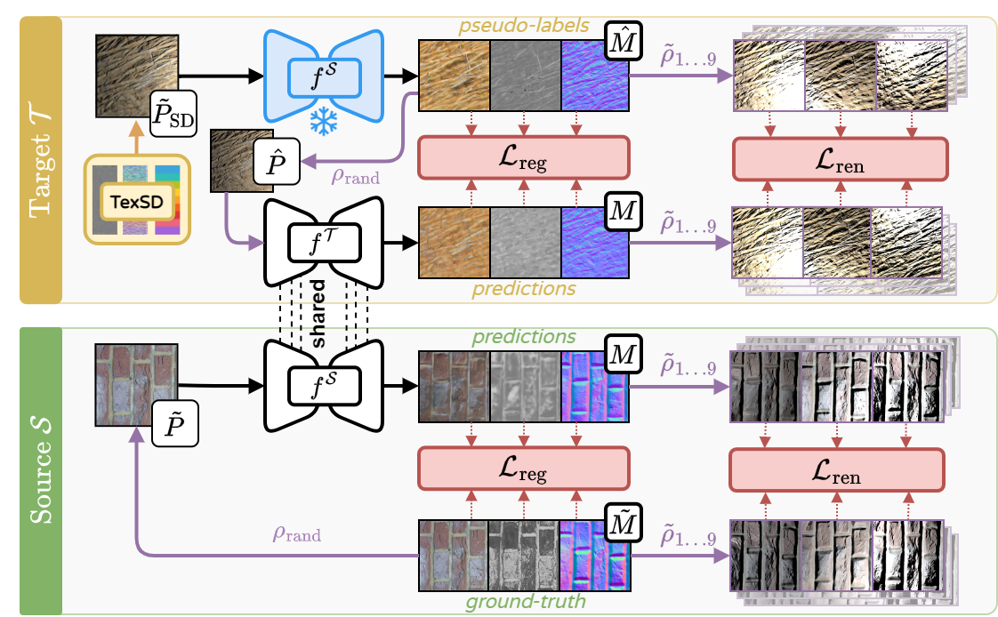
Figure 4: SVBRDF Unsupervised Domain Adaptation. We train a decomposition network $f$ on labeled SVBRDF materials $\mathcal{S}$ and unlabeled target data $\mathcal{T}$ from our novel TexSD dataset. Ultimately, $\mathcal{T}$ acts as a domain bridge between the SVBRDF dataset and the real domain, i.e., patches generated from our extraction method (cf. Sec. 3.2). We enforce both regression and rendering losses on $\mathcal{S}$ and $\mathcal{T}$ using pseudo-maps $\hat{M}$ extracted by the source-only model $f^{\mathcal{S}}$ (top). The final adapted model is denoted $f^{\mathcal{T}}$.

We now seek to decompose each generated RGB-only texture from $P_{\text{SD}}$ into intrinsics $M=\{A,R,N\}$. From Sec. 3.1, a decomposition network $f$ can be trained on a SVBRDF dataset and used on our generated textures $P_{\text{SD}}$. Although these are much closer, than $\mathbf{\mathcal{R}}$, to actual renderings of SVBRDF datasets, $f$ still suffers from a distribution shift. We address this problem as an unsupervised domain adaptation (UDA) $\mathcal{S}{\mapsto}\mathcal{T}$ where the source domain $\mathcal{S}$ consists of materials with SVBRDF labels, and the target domain $\mathcal{T}$ is composed of diffusion-generated RGB textures.

Source training. We train our source model $f^{\mathcal{S}}$ by enforcing a reconstruction loss on ground truth maps $\tilde{M}$ and a multi-view rendering loss with 9 lighting configurations, denoted $\rho_{1\dots 9}$. Explicitly, we optimize $f^{\mathcal{S}}$ by minimizing $\mathcal{L}_{\text{reg}}$ and $\mathcal{L}_{\text{ren}}$ defined in Eq. 2 with:

$$\lambda\mathcal{L}_{\text{reg}}(M,\tilde{M})+\mathcal{L}_{\text{ren}}(M,\tilde{M})\,$$ (3)

where $M=f^{\mathcal{S}}(\tilde{P})$ and $\tilde{P}$ the rendering of $\tilde{M}$ with a random lighting $\rho_{\text{rand}}$. Ground truth maps $\tilde{M}\in\mathcal{S}$ are obtained from any SVBRDF library such as ACG [1].

TexSD. To bridge the gap with SVBRDF libraries, we first generate training material textures in the target domain by prompting the text-to-image model with PromptsGen, e.g., “realistic $S^{c}$ texture in top view”, replacing $S^{c}$ with a class name. Notably, we do not rely on finetuning, but instead only exploit the text-to-image capabilities of large diffusion models and their innate knowledge of material classes. This allows us to construct a dataset, named TexSD, of 9,000 textures generated from a set of 130 classes derived from ACG and ChatGPT proposals [39]. A schematic view is in Fig. 2 (block ‘TexSD’), and details are in the supplementary. Crucially, despite the generation of multiple images per class, these texture images are not multiple views of the same material instance. They are instead single-view variations within a class.

Adaptation. Equipped with TexSD as target domain $\mathcal{T}$, we overcome the ill-posed single-view training (cf. Fig. 3) drawing inspiration from pseudo-labels [26]. We extract pseudo-decomposition maps $\hat{M}=\{\hat{A},\hat{N},\hat{R}\}$ for all textures images $\tilde{P}_{\text{SD}}\in\textbf{TexSD}$ by processing them with our source model $f^{\mathcal{S}}$. This enables pseudo multi-view training on $\mathcal{T}$ with only single view images.

Hence, we adopt Eq. 3 to first train on $\mathcal{S}$ with ground truth $\tilde{M}$, and then finetune concurrently on $\mathcal{S}+\mathcal{T}$, using pseudo-labels $\hat{M}$ for $\mathcal{T}$. An illustration of the training process is shown in Fig. 4. In both stages, SVBRDF inputs are rendered with random lighting conditions $\rho_{\text{rand}}$ to encourage invariance and robustness. At inference, we use $f^{\mathcal{T}}$ to infer the SVBRDF of $P_{\text{SD}}$, leading to material maps $M_{\text{SD}}$.

3.4 Pipeline automation

Our pipeline is readily usable to extract materials from any region $\mathbf{\mathcal{R}}$ of a real-world image. While 3D applications may benefit from user interaction to define $\mathbf{\mathcal{R}}$, we also complement our pipeline with full automation.

To do so, we formalize the problem of defining regions $\{\mathbf{\mathcal{R}}_{1},\cdots,\mathbf{\mathcal{R}}_{N}\}$ on real-world images as a 2D segmentation task. We integrate two segmentation models in our pipeline: the Segment Anything Model (SAM) [25], a large-scale instance segmentation model, and Materialistic [53], a material selection method. In Sec. 4.4, we show how all of these region proposals lead to accurate material extractions.

4 Experiments

We study the performance of $\color[rgb]{0.09,0.45,0.27}\mathsf{Material~{}Palette}$ along four main axes: i) Measuring the quality of our generated textures with respect to textures scraping techniques (Sec. 4.2); ii) Quantifying our SVBRDF adaptation scheme on real material textures (Sec. 4.3); iii) Evaluating the quality of our extracted materials end-to-end (Sec. 4.4); iv) Through exhaustive rendering of 3D scenes with our materials. We also ablate our method in Sec. 4.5 and demonstrate the usage of our material palette for 3D editing in Sec. 4.6.

4.1 Experimental details

Networks.  We use Stable Diffusion [46] for texture extraction, training a LoRA [22] Dreambooth [49] for learning $S^{*}$. Optimization times take around 3-5 min per learned $S^{*}$ on a Tesla V100-16GB. When learning $S^{*}$, PromptTrain is set to “an object with $S^{*}$ texture” while for inference it is chosen randomly among PromptsGen (see Fig. 10). To ensure tileability and high resolution generation, we roll the latent tensor by a random amount at every timestep of the diffusion process [56]. We apply Poisson solving [40] to remove seams remaining on the borders. We directly sample textures up to 1024px while for higher resolutions, we batch-decode the latent code and blend overlapping patches using a weighted average. For $f$, we use a multi-head CNN [34] with U-Net [47], ResNet-101 [20] backbone, and custom decoders with alternating upsample-conv layers. Details are in the supplementary material.

	Patch-based					Region-based
Image	Patch		DeepTex[17]	Quilting [13]	PSGAN [6]	Region	Li et al. [28]	Ours (2048x2048)

Figure 5: Textures extraction. We compare texture extracted from natural images with 4 baselines being patch-based or region-based. Different from baselines, our method is based on a learned concept $S^{*}$ which, when used for generating samples, corrects artifacts, is not limited to a fixed resolution and is fully tileable, resulting in homogeneous textures. For ease of comparison, we show outputs at 2048x2048 along a x2 and x4 zoom. Images are downscaled for visualization purposes.

Public datasets.  We leverage three SVBRDF libraries (AmbientCG [1], PolyHaven [41], CGBookcase [8]) and one material segmentation dataset (OpenSurfaces [5]).
AmbientCG (ACG) contains 2000 high-resolution PBR materials obtained from real-world captures with special apparatus, procedural generation, or image approximation. It includes around 50 material classes. We use the high-resolution 2k textures from ACG to train all source models.
PolyHaven (PH) and CGBookcase (CGB) are smaller libraries composed of 320 materials each. We use them as evaluating sets to validate our adaptation method.
OpenSurfaces (OS) is an image dataset including dense material annotations. We use 14 overlapping classes with ACG and use a subset for end-to-end evaluation.

TexSD dataset.  Our new TexSD dataset (Sec. 3.3) for adaptation. It totals 9,000 textures generated at 1024x1024 by prompting Stable Diffusion [46] with PromptsGen and 130 class names. We detail it in the supplementary.

4.2 Texture extraction

We showcase our text-to-image texture extraction (Sec. 3.2) and existing techniques in Fig. 5. We compare qualitatively with [28] while also providing GAN-based baselines [6], methods inspired by style transfer [17] or image quilting [14]. For a fair comparison, we show outputs from our method using the same regions as [28].
Even though [28] outperforms older methods, it presents artifacts (last two rows) making images unsuitable for material extraction. Moreover, the extracted textures are non-tileable and entangle geometry and lighting. In particular in the second row, the texture of [28] replicates the shading of the input coral image. Our method dramatically differs as it is able to map input images to plausible material textures, removing geometry and lighting while remaining devoid of artifacts. Importantly, we can generate any variations of tileable samples, at any resolution. Ultimately, this shows the inadequacy of prior extraction methods for extracting tileable high-resolution texture patches suitable for decomposition and rendering purposes.

			MSE ($10e1$) $\downarrow$				SSIM $\uparrow$				$\mathbf{\Delta}$% $\uparrow$
	method	DA	A	N	R		A	N	R		ANR
PH ID	Deep Materials [9]		0.264	0.380	0.453		0.379	0.235	0.358
	$\scriptsize{\mathcal{S}\text{ource-only}}$		0.083	0.300	0.475		0.610	0.304	0.458		$\Rsh$
	SurfaceNet [55]	✓	0.071	0.298	0.427		0.626	0.304	0.472		+5.18
	ours	$\checkmark$	0.069	0.291	0.443		0.630	0.309	0.476		+5.87
CGB ID	Deep Materials [9]		0.590	0.465	1.940		0.392	0.228	0.346
	$\mathcal{S}\text{\scriptsize{ource-only}}$		0.098	0.221	0.555		0.662	0.437	0.476		$\Rsh$
	SurfaceNet [55]	$\checkmark$	0.101	0.230	0.615		0.657	0.445	0.471		-3.00
	ours	$\checkmark$	0.084	0.219	0.588		0.669	0.457	0.482		+2.62
PH OOD	Deep Materials [9]		0.264	0.380	0.453		0.379	0.235	0.358
	$\mathcal{S}\text{\scriptsize{ource-only}}$		0.065	0.247	0.439		0.608	0.284	0.518		$\Rsh$
	SurfaceNet [55]	$\checkmark$	0.053	0.250	0.415		0.608	0.283	0.524		+3.94
	ours	$\checkmark$	0.053	0.246	0.409		0.618	0.288	0.531		+5.24

Table 1: DA evaluation. Performances on In-Distribution (ID, top) and Out-of-Distribution (OOD, bottom). $\Delta$ measures the relative performance over {A,N,R} w.r.t. the ACG-only model. DA refers to methods using domain adaptation strategies. Our adaptation succeeds at preserving generalization abilities on OOD samples, while SurfaceNet [55] has slightly lower gains on OOD.

	Source-only (ACG)				Ours $\text{ACG}\mapsto\text{SD}$
Image	A	N	R	3D	A	N	R	3D

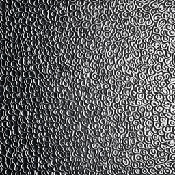
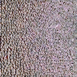
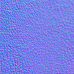
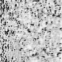
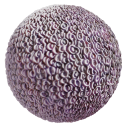
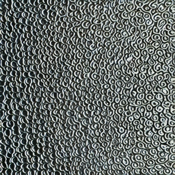
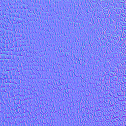
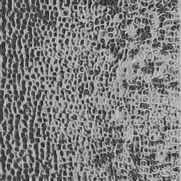
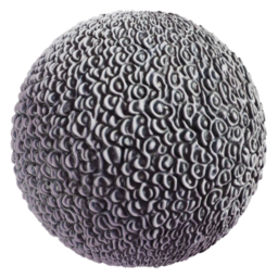
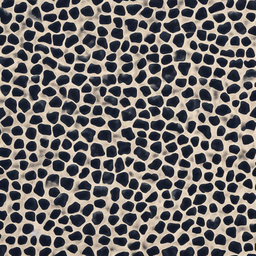
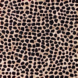
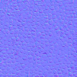
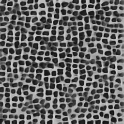
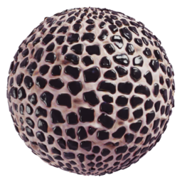
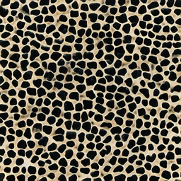
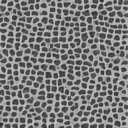
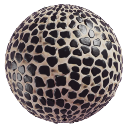
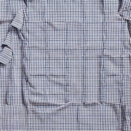
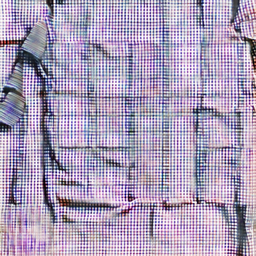
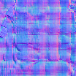
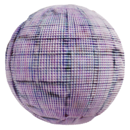
Figure 6: Qualitative results. Comparison between source-only training (ACG) and our ($\text{ACG}\mapsto\text{SD}$) adaptation on unseen SD samples. We notice that source-only overestimates N and R and exhibits color shift in A. This results in a lower-quality 3D render.

4.3 SVBRDF decomposition

We now focus on our proposed UDA pipeline for decomposition (Sec. 3.3). Since our TexSD dataset does not come with associated SVBRDF ground truths, we rather evaluate on two additional $\mathcal{S}{\mapsto}\mathcal{T}$ scenarios: $\text{ACG}{\mapsto}\text{PH}$ and $\text{ACG}{\mapsto}\text{CGB}$. This allows us to measure the adaptation effectiveness on the target set $\mathcal{T}$ w.r.t. ground truth annotations. We report standard metrics: Mean Squared Error ($MSE$ $\downarrow$) and Structural Similarity Index ($SSIM$ $\uparrow$) [58]. For a refined comparison, we evaluate common classes in $\mathcal{S}$ and $\mathcal{T}$ as In-Distribution (ID), resulting in 53 and 58 materials for PH and CGB, respectively.

We propose three baselines. First, we evaluate Deep Materials [9] as an off-the-shelf decomposition network. We also compare with an ACG $\mathcal{S}\text{ource-only}$ model, serving as lower bound. Then, we implement SurfaceNet [55] with our architecture and finetune the original ACG model for both SurfaceNet and ours. Results in Tab. 1 (top) suggest that we improve consistently the decomposition. Considering the richer PH material ontology, we also evaluate the 47 classes of materials Out-Of-Distribution (OOD). In Tab. 1 we obtain only a low-performance OOD drop (bottom) compared to ID (top), exhibiting better generalization than baselines. Furthermore, we show in Fig. 6 a visual comparison of ‘Ours $\text{ACG}{\mapsto}\text{SD}$’ vs ‘source-only (ACG)’, on TexSD unseen samples. It shows our adaptation better decomposes images, ultimately producing more realistic 3D renderings.

		LPIPS $\downarrow$
	$\mathbf{\mathcal{R}}$	A	N	R
upper bound		0.8288	0.5915	0.7255
Ours	OS masks [5]	0.7959	0.5730	0.7142
	SAM [25]	0.8048	0.5692	0.7096
	Materialistic [53]	0.8077	0.5678	0.7169
lower bound		0.6789	0.4629	0.6843

		CLIP Classif. $\uparrow$
	$\rho(M)$	top-1	top-5
	ACG	47.78	85.88
Ours	OS masks [5]	47.03	85.12
	SAM [25]	43.71	80.83
	Materialistic [53]	50.89	86.82

Table 2: Resemblance to SVBRDF dataset. We evaluate our extracted materials with various regions proposals w.r.t. materials from ACG (left). We also report zero-shot classification on ACG (right) which measures ability of CLIP to classify the class of the re-rendered material [42]. Both results demonstrate that our materials have coherent class-wise characteristics without class annotations, irrespective of the segmenter used.

Materialistic		SAM		User-defined

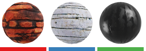
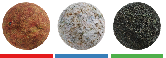
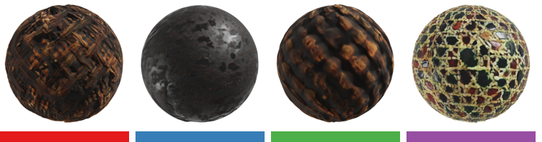
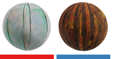
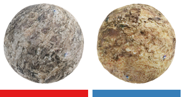
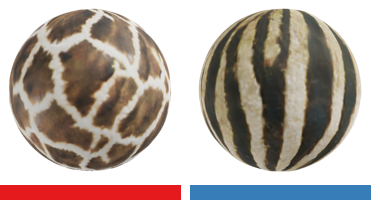
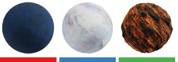
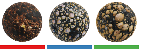
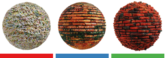
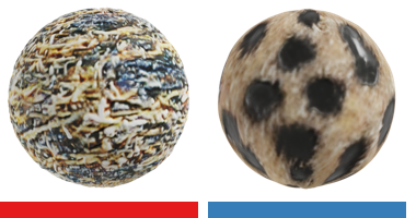
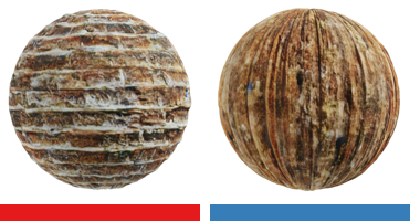
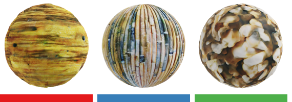
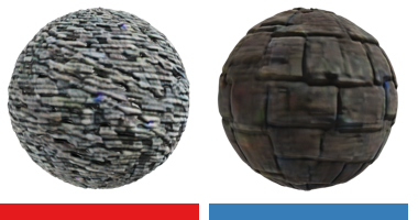
Figure 7: Material palettes. We show qualitative results of $\color[rgb]{0.09,0.45,0.27}\mathsf{Material~{}Palette}$ on images gathered on the internet with regions extracted using Materialistic, SAM, or defined by the user.

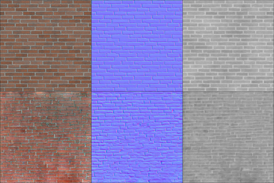
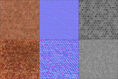
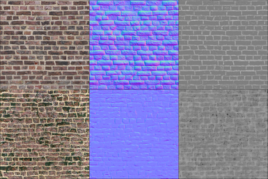
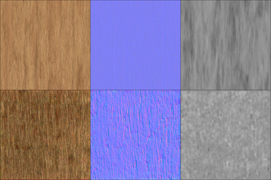
		LPIPS $\downarrow$ $P$ A N R SD rand. 0.8163 0.6895 0.7441 ours (user) 0.6839 0.6254 0.5951 ACG rand. 0.6547 0.4508 0.5600

Figure 8: End to end evaluation. We edit 3D scenes with ACG materials rendering different scenes and viewpoints. This allows us to compare $\color[rgb]{0.09,0.45,0.27}\mathsf{Material~{}Palette}$ extractions w.r.t. ACG ground truth, and quantify our end-to-end performance (extraction $+$ decomposition). Extracted regions are shown in top-left insets.

4.4 Material extraction

Given the lack of datasets combining real scenes with region-wise materials annotations, we highlight the complexity of evaluating all components of our method together.

Resemblance to SVBRDFdataset.  We design experiments using OpenSurfaces (OS) and ACG, allowing us to understand if $\color[rgb]{0.09,0.45,0.27}\mathsf{Material~{}Palette}$ preserves the expected characteristics of a material region. Considering that datasets class ontologies differ, we map OS and ACG classes to a common set of 14 materials $C_{m}$, detailed in the supplementary, in which OS classes are grouped following [60].

In a first experiment, we use OS ground truth, i.e. user-annotated material segmentation masks, as $\mathcal{R}$, and automatically extract the associated materials $M_{\text{SD}}$ with $\color[rgb]{0.09,0.45,0.27}\mathsf{Material~{}Palette}$. Given that in the OS ground truth the material class $c$ of $\mathcal{R}$ is known (but not the intrinsics), we compare the extracted $M_{\text{SD}}$ with those of materials of the same class in ACG. We define an upper bound by evaluating the same extracted materials but on all other materials in ACG. Intuitively, if results are better than the upper bound, we correctly mapped the appearance of a particular material class to visual features specific to that class. In other words, a material labeled as ‘brick’ in a natural image should lead to extracted maps more similar to ‘brick’ samples in ACG, than to other classes such as ‘wood’. In practice, the evaluation is conducted by sampling 100 $\{M_{\text{SD}},\tilde{M}\}$ pairs and evaluating LPIPS [64] between them (lower is better), for each of the 14 material classes. Considering class $c\in C_{m}$, Ours will evaluate $\{M_{\text{SD}}^{c},\tilde{M}^{c}\}$ pairs $\forall c\in C_{m}$, while the upper bound will have $\{M_{\text{SD}}^{c},\tilde{M}^{\bar{c}}\}$ where $\bar{c}$ is a random ${\bar{c}}\neq c$. The reported LPIPS values are averaged over all classes. From Tab. 2 (left), ‘Ours-OS Masks’ improves performance over the upper bound, proving the effectiveness of our method. Additionally, we propose a lower bound, following our pipeline but using $\{M_{\text{ACG}}^{c},\tilde{M}^{c}\}$ where $M_{\text{ACG}}$ are estimated ACG maps from single-view samples of class $c$. We also evaluate the impact on material extraction of our automated pipeline using either SAM [25] or Materialistic [53] as region segmenters (Sec. 3.4). We highlight how in all setups we achieve comparable performance, always improving over the lower bound.

In a second experiment, we propose an evaluation with CLIP [42]. We combine all generated textures of $c\in C_{m}$ with PromptsGen (cf. Sec. 4.5) and evaluate the CLIP ViT-B/32 zero-shot classification performance of all rendered $M_{\text{SD}}$ with random illumination. We do the same for all ground truth $\tilde{M}$ in ACG. In Tab. 2 (right) we report average comparable accuracies, suggesting that we successfully render similar materials to existing PBR datasets, $\forall c\in C_{m}$.

Qualitative evaluation.  In Fig. 7 we visualize web-scraped images and the materials extracted by $\color[rgb]{0.09,0.45,0.27}\mathsf{Material~{}Palette}$ using regions from SAM [25], Materialistic [53] or a User input. Each material is rendered on a 3D sphere in Blender with a color below matching its region color. Given the task complexity, we emphasize the quality of the extraction for a wide variety of complex materials: bricks, tiles, skins, fur, etc. In particular, we highlight the quality of bricks in (a) as well as in (j) and (j) with a different segmenter, and more astonishingly in the small roof region of (o) . In natural images, materials also match appearances such as crocodile skin  (i) , or fur of jaguar (k) , giraffe (g) and zebra (g) . Other noticeable results are the complex mosaic pattern (c) or damaged wall (d) and (d) .

End-to-end re-rendering.  We also design a challenging end-to-end evaluation leveraging realistic 3D scenes. Through automatic edition we replace some 3D objects material with a PBR material of ACG, thus rendering a total of 174 images (2 scenes, 4 views) comprising 10 materials for each of the 16 dominant classes of ACG. As the latter comes with SVBRDF ground truths, we compare them with our $\color[rgb]{0.09,0.45,0.27}\mathsf{Material~{}Palette}$ extractions on the rendered images with ad-hoc user-input regions. Visuals in Fig. 8 show side-by-side renderings, each with ACG ground truth (top) and our extractions (bottom). Our materials capture the main characteristics though we observe some over/under saturation, highlighting the task complexity. Moreover, table inset in Fig. 8 compares LPIPS($\downarrow$) vs ground truth ACG for either a ‘SD random’ generation prompted with the true class, or a random ACG material of the true class. Notably, our materials are much closer to ACG than SD generation, demonstrating the benefit of our pipeline over text-to-image.

	region	$c_{in}=128$		$c_{in}=256$		$c_{in}=512$
$c_{x}=64$
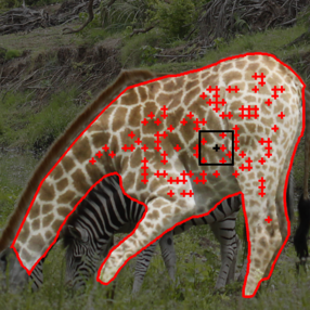
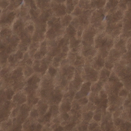
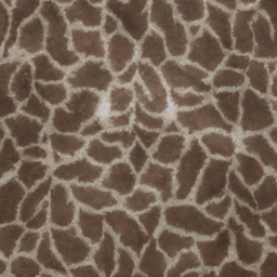
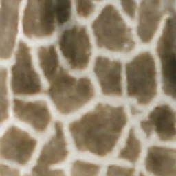
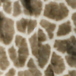
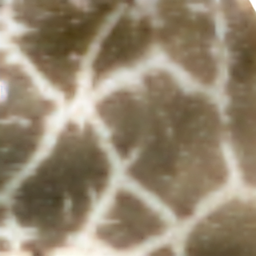
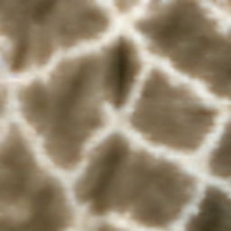
$c_{x}=128$

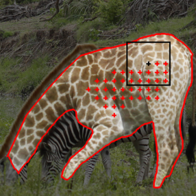
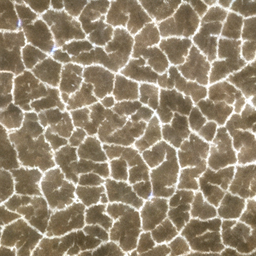
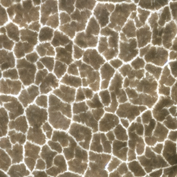
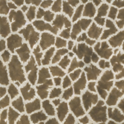
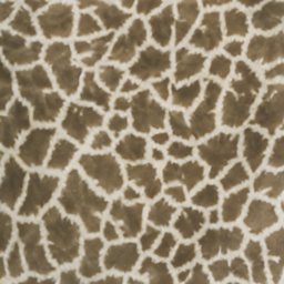
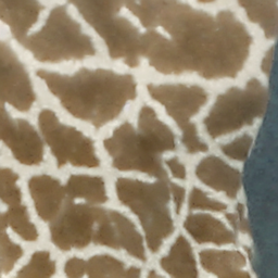
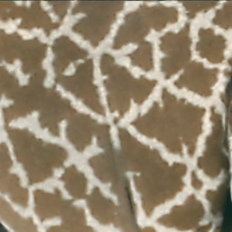
	“a photo of $\textbf{S}^{*}$ texture”		“$\textbf{S}^{*}$”		“a photo of a $\textbf{S}^{*}$”		“an object with $\textbf{S}^{*}$ texture”
$\blacksquare$
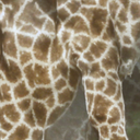
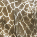
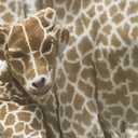
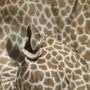
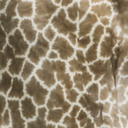
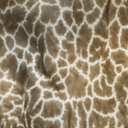
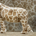
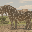
$\blacksquare$
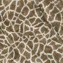
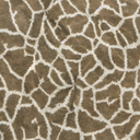
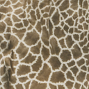
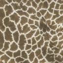
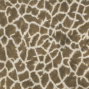
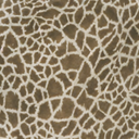
$\blacksquare$

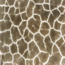
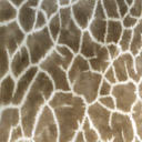
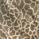
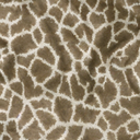
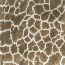
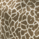
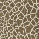
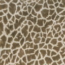
Figure 9: Inversion ablation. We show how crop and upsampling sizes affect SD generation results (top). Effects of PromptTrain for learning $\textbf{S}^{*}$ are also given (bottom). For all four inversions, we provide generations using the templates $\blacksquare$, $\blacksquare$, and $\blacksquare$ (cf. Fig. 10). We highlight in green the parameters used.

		FID $\downarrow$				KID $\downarrow$
	Prompt templates	A	N	R		A	N	R
$\blacksquare$	“a photo of a $\textbf{S}^{c}$”	1.89	1.74	1.83		2.60	6.52	3.75
$\blacksquare$	“a $\textbf{S}^{c}$ material”	1.83	1.60	1.67		2.38	5.42	2.74
$\blacksquare$	“a $\textbf{S}^{c}$ texture”	1.72	1.54	1.63		1.82	5.27	2.86
$\blacksquare$	“realistic $\textbf{S}^{c}$ texture in top view”	1.55	1.27	1.59		1.54	3.34	3.32
$\blacksquare$	“high resolution realistic $\textbf{S}^{c}$ texture in top view”	1.55	1.30	1.55		1.71	3.48	3.34

$\textbf{S}^{c}$	$\blacksquare$	$\blacksquare$	$\blacksquare$	$\blacksquare$	$\blacksquare$	ACG
Paper
Pav. Stones

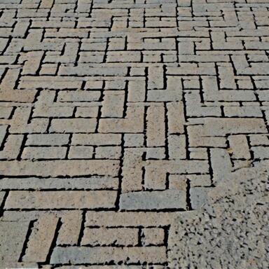
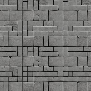
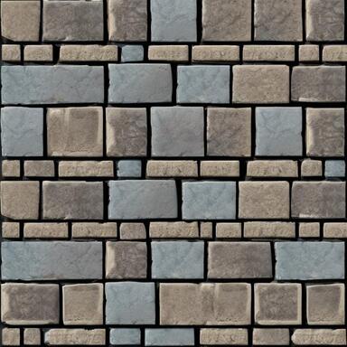
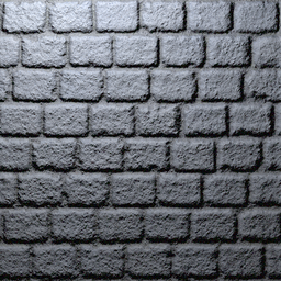
Figure 10: Prompt generation. We compare prompt templates when generating using class names as $\textbf{S}^{c}$. With a more detailed prompt and the word “texture”, we are able to generate images similar to the ones in ACG. We report FID $\cdot 10^{-2}$ and KID $\cdot 10^{2}$.

“classroom”			“flat-front”				“flat-back”
5pt. 5pt. 5pt.

Figure 11: Scene editing. We edit objects (top-left insets) of 3D scenes using materials extracted from real-world images.

4.5 Ablations

Inversion.  Considering we face objects of varying sizes, we motivate our need for scale adaptive crop extraction. In Fig. 9 (top), we show the crop size $c_{x}$ and training input size $c_{in}$ (i.e., upsampling size). Considering that crops have a much lower resolution than the pre-trained SD v1.5 inputs (512px), we make two choices: (i) extract crops with largest $c_{x}$ possible within $\mathbf{\mathcal{R}}$, and (ii) finetune SD at a lower resolution ($c_{in}=256$). This minimizes the input distortion while retaining good generation at 512px and beyond.

Additionally, we evaluate Fig. 9 (bottom) the choice of PromptTrain when learning $S^{*}$ by showing generations using three prompts from Fig. 10. While choosing PromptTrain (row-wise) plays less than PromptsGen, we use “an object with $\textbf{S}^{*}$ texture” when training. This motivates our choices for learning $S^{*}$ (Sec. 3.2).

Prompt engineering.  We find that choosing the correct PromptsGen allows generating material images with the correct appearance. We ablate in Fig. 10 (top) different prompts by sampling 10 images per ACG class and processing them with our decomposition (Sec. 3.3). We then evaluate FID and KID against ACG annotations and rendered images. We find that the word “texture” improves synthesis over generic templates and removes additional context favoring top-view appearance. Furthermore, the text-to-image generation benefits from additional adjectives. Visual comparison of generated samples is in Fig. 10 (bottom).

4.6 3D Scene editing.

We consider the extracted materials for scene editing applications. In Sec. 4.4, we present renderings of 3D scenes, replacing materials of objects (highlighted in insets) with ones extracted in real-world images with $\color[rgb]{0.09,0.45,0.27}\mathsf{Material~{}Palette}$. Note the realism of our jaguar (middle) and giraffe (right) sofas, or the bamboo wall (left).

5 Discussion

We introduced  $\color[rgb]{0.09,0.45,0.27}\mathsf{Material~{}Palette}$, a comprehensive approach designed to extract tileable, high-resolution PBR materials from single real-world images. Although capable of extracting accurate materials, our method faces some unexpected limitations. For example, while prior methods may struggle at regressing complex patterns we found it more challenging to capture simple uniform materials. In such cases, the concept collapses, leading to color artifacts, common in diffusion models. Another more predictable issue, involves illumination ambiguities – particularly noticeable in shaded surfaces – causing inconsistent colors. Lastly, $\color[rgb]{0.09,0.45,0.27}\mathsf{Material~{}Palette}$ is capable of making some geometric corrections, but cannot rectify slanted surfaces or account for strong distortion (perspective, lenses, depth of field). Addressing these shortcomings calls for further refinements. $\color[rgb]{0.09,0.45,0.27}\mathsf{Material~{}Palette}$ shows very promising results on a newly introduced challenging task. We hope our work sparks interesting research in the same direction.

Acknowledgment. This research project was funded by the French project SIGHT (ANR-20-CE23-0016). It was performed using HPC resources from GENCI–IDRIS (Grant 2023-AD011014389).

References

- AmbientCG [2017] AmbientCG. Pbr repository. https://www.ambientcg.com, 2017. Accessed: 2023-04-01.
- Asselin et al. [2020] Louis-Philippe Asselin, Denis Laurendeau, and Jean-François Lalonde. Deep svbrdf estimation on real materials. In 3DV, 2020.
- Barron and Malik [2013] Jonathan T Barron and Jitendra Malik. Intrinsic scene properties from a single rgb-d image. In CVPR, 2013.
- Bartels et al. [2019] Joseph R Bartels, Jian Wang, William Whittaker, Srinivasa G Narasimhan, et al. Agile depth sensing using triangulation light curtains. In ICCV, 2019.
- Bell et al. [2013] Sean Bell, Paul Upchurch, Noah Snavely, and Kavita Bala. OpenSurfaces: A richly annotated catalog of surface appearance. In ACM TOG, 2013.
- Bergmann et al. [2017] Urs Bergmann, Nikolay Jetchev, and Roland Vollgraf. Learning texture manifolds with the periodic spatial gan. In ICML, 2017.
- Cazenavette et al. [2022] George Cazenavette, Tongzhou Wang, Antonio Torralba, Alexei A Efros, and Jun-Yan Zhu. Wearable imagenet: Synthesizing tileable textures via dataset distillation. In CVPR-W, 2022.
- CGBookCase [2019] CGBookCase. Pbr repository. https://www.cgbookcase.com, 2019. Accessed: 2023-04-01.
- Deschaintre et al. [2018] Valentin Deschaintre, Miika Aittala, Fredo Durand, George Drettakis, and Adrien Bousseau. Single-image svbrdf capture with a rendering-aware deep network. ACM TOG, 2018.
- Deschaintre et al. [2020] Valentin Deschaintre, George Drettakis, and Adrien Bousseau. Guided fine‐tuning for large‐scale material transfer. Comput. Graph. Forum, 2020.
- Deschaintre et al. [2021] Valentin Deschaintre, Yiming Lin, and Abhijeet Ghosh. Deep polarization imaging for 3d shape and svbrdf acquisition. In CVPR, 2021.
- Diamanti et al. [2015] Olga Diamanti, Connelly Barnes, Sylvain Paris, Eli Shechtman, and Olga Sorkine-Hornung. Synthesis of complex image appearance from limited exemplars. ACM TOG, 2015.
- Efros and Freeman [2001] Alexei A Efros and William T Freeman. Image quilting for texture synthesis and transfer. In ACM TOG, 2001.
- Efros and Leung [1999] Alexei A Efros and Thomas K Leung. Texture synthesis by non-parametric sampling. In ICCV, 1999.
- Gao et al. [2019] Duan Gao, Xiao Li, Yue Dong, Pieter Peers, Kun Xu, and Xin Tong. Deep inverse rendering for high-resolution svbrdf estimation from an arbitrary number of images. ACM TOG, 2019.
- Garon et al. [2019] Mathieu Garon, Kalyan Sunkavalli, Sunil Hadap, Nathan Carr, and Jean-Francois Lalonde. Fast spatially-varying indoor lighting estimation. In CVPR, 2019.
- Gatys et al. [2015] Leon Gatys, Alexander S Ecker, and Matthias Bethge. Texture synthesis using convolutional neural networks. In NeurIPS, 2015.
- Germer et al. [2014] Thomas Germer, Joanne C Zwinkels, and Benjamin K Tsai. Spectrophotometry: Accurate measurement of optical properties of materials. Elsevier, 2014.
- Guarnera et al. [2016] Darya Guarnera, Giuseppe Claudio Guarnera, Abhijeet Ghosh, Cornelia Denk, and Mashhuda Glencross. Brdf representation and acquisition. In Comput. Graph. Forum, 2016.
- He et al. [2015] Kaiming He, Xiangyu Zhang, Shaoqing Ren, and Jian Sun. Deep residual learning for image recognition, 2015.
- Horn [1974] Berthold KP Horn. Determining lightness from an image. CGIP, 1974.
- Hu et al. [2022] Edward J Hu, Yelong Shen, Phillip Wallis, Zeyuan Allen-Zhu, Yuanzhi Li, Shean Wang, Lu Wang, and Weizhu Chen. LoRA: Low-rank adaptation of large language models. In ICLR, 2022.
- Innamorati et al. [2017] Carlo Innamorati, Tobias Ritschel, Tim Weyrich, and Niloy J Mitra. Decomposing single images for layered photo retouching. In Comput. Graph. Forum, 2017.
- Joy and Poullis [2022] Alen Joy and Charalambos Poullis. Multi-view gradient consistency for svbrdf estimation of complex scenes under natural illumination. arXiv, 2022.
- Kirillov et al. [2023] Alexander Kirillov, Eric Mintun, Nikhila Ravi, Hanzi Mao, Chloe Rolland, Laura Gustafson, Tete Xiao, Spencer Whitehead, Alexander C Berg, Wan-Yen Lo, et al. Segment anything. In ICCV, 2023.
- Lee et al. [2013] Dong-Hyun Lee et al. Pseudo-label: The simple and efficient semi-supervised learning method for deep neural networks. In ICML, 2013.
- Li et al. [2017] Xiao Li, Yue Dong, Pieter Peers, and Xin Tong. Modeling surface appearance from a single photograph using self-augmented convolutional neural networks. ACM TOG, 2017.
- Li et al. [2022a] Xueting Li, Xiaolong Wang, Ming-Hsuan Yang, Alexei A Efros, and Sifei Liu. Scraping textures from natural images for synthesis and editing. In ECCV, 2022a.
- Li and Snavely [2018] Zhengqi Li and Noah Snavely. Cgintrinsics: Better intrinsic image decomposition through physically-based rendering. In ECCV, 2018.
- Li et al. [2020] Zhengqin Li, Mohammad Shafiei, Ravi Ramamoorthi, Kalyan Sunkavalli, and Manmohan Chandraker. Inverse rendering for complex indoor scenes: Shape, spatially-varying lighting and svbrdf from a single image. In CVPR, 2020.
- Li et al. [2022b] Zhengqin Li, Jia Shi, Sai Bi, Rui Zhu, Kalyan Sunkavalli, Miloš Hašan, Zexiang Xu, Ravi Ramamoorthi, and Manmohan Chandraker. Physically-based editing of indoor scene lighting from a single image. In ECCV. Springer, 2022b.
- Liao et al. [2019] Zicheng Liao, Kevin Karsch, Hongyi Zhang, and David Forsyth. An approximate shading model with detail decomposition for object relighting. IJCV, 2019.
- Liu et al. [2020] Yunfei Liu, Yu Li, Shaodi You, and Feng Lu. Unsupervised learning for intrinsic image decomposition from a single image. In CVPR, 2020.
- Lopes et al. [2023] Ivan Lopes, Tuan-Hung Vu, and Raoul de Charette. Cross-task attention mechanism for dense multi-task learning. In WACV, 2023.
- Martin et al. [2022] Rosalie Martin, Arthur Roullier, Romain Rouffet, Adrien Kaiser, and Tamy Boubekeur. Materia: Single image high-resolution material capture in the wild. In Comput. Graph. Forum, 2022.
- Monnier et al. [2022] Tom Monnier, Matthew Fisher, Alexei A Efros, and Mathieu Aubry. Share with thy neighbors: Single-view reconstruction by cross-instance consistency. In ECCV, 2022.
- Narihira et al. [2015] Takuya Narihira, Michael Maire, and Stella X Yu. Direct intrinsics: Learning albedo-shading decomposition by convolutional regression. In ICCV, 2015.
- Nichol et al. [2022] Alex Nichol, Prafulla Dhariwal, Aditya Ramesh, Pranav Shyam, Pamela Mishkin, Bob McGrew, Ilya Sutskever, and Mark Chen. Glide: Towards photorealistic image generation and editing with text-guided diffusion models. In ICML, 2022.
- OpenAI [2023] OpenAI. Chatgpt. chat.openai.org, 2023. Accessed: 2023-05-20.
- Pérez et al. [2023] Patrick Pérez, Michel Gangnet, and Andrew Blake. Poisson image editing. In Seminal Graphics Papers: Pushing the Boundaries. SIGGRAPH, 2023.
- PolyHaven [2021] PolyHaven. Pbr repository. https://www.polyhaven.com, 2021. Accessed: 2023-04-01.
- Radford et al. [2021] Alec Radford, Jong Wook Kim, Chris Hallacy, Aditya Ramesh, Gabriel Goh, Sandhini Agarwal, Girish Sastry, Amanda Askell, Pamela Mishkin, Jack Clark, Gretchen Krueger, and Ilya Sutskever. Learning transferable visual models from natural language supervision, 2021.
- Ramesh et al. [2021] Aditya Ramesh, Mikhail Pavlov, Gabriel Goh, Scott Gray, Chelsea Voss, Alec Radford, Mark Chen, and Ilya Sutskever. Zero-shot text-to-image generation. In ICML, 2021.
- Ramesh et al. [2022] Aditya Ramesh, Prafulla Dhariwal, Alex Nichol, Casey Chu, and Mark Chen. Hierarchical text-conditional image generation with clip latents. arXiv, 2022.
- Rodriguez-Pardo et al. [2023] Carlos Rodriguez-Pardo, Henar Domínguez-Elvira, David Pascual-Hernández, and Elena Garces. Umat: Uncertainty-aware single image high resolution material capture. In CVPR, 2023.
- Rombach et al. [2022] Robin Rombach, Andreas Blattmann, Dominik Lorenz, Patrick Esser, and Björn Ommer. High-resolution image synthesis with latent diffusion models. In CVPR, 2022.
- Ronneberger et al. [2015] Olaf Ronneberger, Philipp Fischer, and Thomas Brox. U-net: Convolutional networks for biomedical image segmentation. In MICCAI, 2015.
- Rosenberger et al. [2009] Amir Rosenberger, Daniel Cohen-Or, and Dani Lischinski. Layered shape synthesis: automatic generation of control maps for non-stationary textures. ACM TOG, 2009.
- Ruiz et al. [2023] Nataniel Ruiz, Yuanzhen Li, Varun Jampani, Yael Pritch, Michael Rubinstein, and Kfir Aberman. Dreambooth: Fine tuning text-to-image diffusion models for subject-driven generation. In CVPR, 2023.
- Saharia et al. [2022] Chitwan Saharia, William Chan, Saurabh Saxena, Lala Li, Jay Whang, Emily L Denton, Kamyar Ghasemipour, Raphael Gontijo Lopes, Burcu Karagol Ayan, Tim Salimans, et al. Photorealistic text-to-image diffusion models with deep language understanding. In NeurIPS, 2022.
- Sauer et al. [2023] Axel Sauer, Tero Karras, Samuli Laine, Andreas Geiger, and Timo Aila. Stylegan-t: Unlocking the power of gans for fast large-scale text-to-image synthesis. In ICML, 2023.
- Sengupta et al. [2019] Soumyadip Sengupta, Jinwei Gu, Kihwan Kim, Guilin Liu, David W Jacobs, and Jan Kautz. Neural inverse rendering of an indoor scene from a single image. In ICCV, 2019.
- Sharma et al. [2023] Prafull Sharma, Julien Philip, Michaël Gharbi, William T. Freeman, Fredo Durand, and Valentin Deschaintre. Materialistic: Selecting similar materials in images. In ACM TOG, 2023.
- Tang et al. [2012] Yichuan Tang, Ruslan Salakhutdinov, and Geoffrey Hinton. Deep lambertian networks. arXiv, 2012.
- Vecchio et al. [2021] Giuseppe Vecchio, Simone Palazzo, and Concetto Spampinato. Surfacenet: Adversarial svbrdf estimation from a single image. In ICCV, 2021.
- Vecchio et al. [2023a] Giuseppe Vecchio, Rosalie Martin, Arthur Roullier, Adrien Kaiser, Romain Rouffet, Valentin Deschaintre, and Tamy Boubekeur. Controlmat: A controlled generative approach to material capture. arXiv, 2023a.
- Vecchio et al. [2023b] Giuseppe Vecchio, Renato Sortino, Simone Palazzo, and Concetto Spampinato. Matfuse: Controllable material generation with diffusion models, 2023b.
- Wang et al. [2004] Zhou Wang, Alan C Bovik, Hamid R Sheikh, and Eero P Simoncelli. Image quality assessment: from error visibility to structural similarity. T-IP, 2004.
- Wu et al. [2020] Shangzhe Wu, Christian Rupprecht, and Andrea Vedaldi. Unsupervised learning of probably symmetric deformable 3d objects from images in the wild. In CVPR, 2020.
- Xiao et al. [2018] Tete Xiao, Yingcheng Liu, Bolei Zhou, Yuning Jiang, and Jian Sun. Unified perceptual parsing for scene understanding. In ECCV, 2018.
- Xu et al. [2018] Tao Xu, Pengchuan Zhang, Qiuyuan Huang, Han Zhang, Zhe Gan, Xiaolei Huang, and Xiaodong He. Attngan: Fine-grained text to image generation with attentional generative adversarial networks. In CVPR, 2018.
- Yeh et al. [2022] Yu-Ying Yeh, Zhengqin Li, Yannick Hold-Geoffroy, Rui Zhu, Zexiang Xu, Miloš Hašan, Kalyan Sunkavalli, and Manmohan Chandraker. Photoscene: Photorealistic material and lighting transfer for indoor scenes. In CVPR, 2022.
- Zhang et al. [2017] Han Zhang, Tao Xu, Hongsheng Li, Shaoting Zhang, Xiaogang Wang, Xiaolei Huang, and Dimitris N Metaxas. Stackgan: Text to photo-realistic image synthesis with stacked generative adversarial networks. In ICCV, 2017.
- Zhang et al. [2018] Richard Zhang, Phillip Isola, Alexei A Efros, Eli Shechtman, and Oliver Wang. The unreasonable effectiveness of deep features as a perceptual metric. In CVPR, 2018.
- Zhou et al. [2019] Hao Zhou, Xiang Yu, and David W Jacobs. Glosh: Global-local spherical harmonics for intrinsic image decomposition. In ICCV, 2019.
- Zhu et al. [2019] Minfeng Zhu, Pingbo Pan, Wei Chen, and Yi Yang. Dm-gan: Dynamic memory generative adversarial networks for text-to-image synthesis. In CVPR, 2019.