Mission-driven Exploration for Accelerated Deep Reinforcement Learning with Temporal Logic Task Specifications

Abstract

This paper addresses the problem of designing optimal control policies for mobile robots with mission and safety requirements specified using Linear Temporal Logic (LTL). We consider robots with unknown stochastic dynamics operating in environments with unknown geometric structure. The robots are equipped with sensors allowing them to detect obstacles. Our goal is to synthesize a control policy that maximizes the probability of satisfying an LTL-encoded task in the presence of motion and environmental uncertainty. Several deep reinforcement learning (DRL) algorithms have been proposed recently to address similar problems. A common limitation in related works is that of slow learning performance. In order to address this issue, we propose a novel DRL algorithm, which has the capability to learn control policies at a notably faster rate compared to similar methods. Its sample efficiency is due to a mission-driven exploration strategy that prioritizes exploration towards directions that may contribute to mission accomplishment. Identifying these directions relies on an automaton representation of the LTL task as well as a learned neural network that (partially) models the unknown system dynamics. We provide comparative experiments demonstrating the efficiency of our algorithm on robot navigation tasks in unknown environments.

I Introduction

Deep Reinforcement learning (DRL) has been successfully applied to synthesize control policies for autonomous systems in the presence of motion, sensing, and environmental uncertainty [1, 2]. Typically, in DRL, control objectives are specified as reward functions. However, specifying reward-based objectives can be highly non-intuitive, especially for complex tasks, while poorly designed rewards can significantly compromise system performance [3]. To address this challenge, formal languages, such as Linear Temporal logic (LTL), have recently been leveraged. LTL provides a natural encoding of tasks that would have been very hard to define using Markovian rewards [4]; e.g., consider a navigation task that requires visiting regions of interest in a specific order.

Several model-free DRL methods for LTL objectives have been proposed recently; see e.g., [5, 6, 7, 8, 9, 10, 11, 12, 13]. Common in most of these works is that they explore randomly a product state space that grows exponentially as the size of the robot state space and the task complexity increase. This results in a slow learning process which becomes more pronounced by the sparse rewards that are often used to synthesize policies with probabilistic satisfaction guarantees[8]. To expedite learning, reward engineering approaches augmenting the reward signal have been proposed [14, 15, 16, 17, 18, 19, 20]. For instance, hierarchical DRL relies on assigning non-zero rewards to intermediate goals. However, this may result in sub-optimal policies with respect to the original task [21]. Also, augmenting the reward signal for temporal logic tasks may compromise probabilistic correctness of the learned policies [8].

Model-based RL methods for LTL objectives have also been proposed in [22, 23, 24]. These works leverage a learned system model, captured by a Markov Decision Process (MDP), to synthesize optimal policies within a finite number of iterations. As a result, they are more sample-efficient than model-free approaches. Nevertheless, these works typically consider MDPs with discrete state/action spaces resulting in limited applicability/scalability, especially, for robot control applications that often involve continuous spaces.

In this paper, we propose a new accelerated DRL algorithm to generate control policies for mobile robots with unknown stochastic dynamics that have to accomplish LTL-encoded tasks in environments with unknown geometric structure. The robot-environment interaction is modeled as an unknown MDP with continuous state space and discrete action space (modeling e.g., robot motion primitives). Our goal is to learn a control policy for the MDP that maximizes the probability of satisfying the assigned LTL task. Our approach builds upon Deep Q-Networks (DQN) [25]. The major difference with standard DQN lies in our proposed exploration strategy. Particularly, we propose a novel stochastic policy -that extends $\epsilon$-greedy policies- consisting of (i) an exploitation phase and (ii) mission-driven exploration strategy. The latter, instead of randomly exploring the state space, prioritizes exploration towards directions that may contribute to task satisfaction. Identifying these directions leverages the logical task structure but it requires (partial) knowledge of the system dynamics which is not available. We address this by learning a surrogate system model using a neural network. We provide comparative experiments on robot navigation tasks demonstrating that our algorithm outperforms, in terms of sample efficiency, DQN as well as actor-critic algorithms. We emphasize that the proposed stochastic policy can be coupled with any existing deep temporal difference learning framework [26, 27] as well as with any reward augmentation method, discussed earlier, to further enhance sample-efficiency. The latter holds since our exploration strategy is agnostic to the reward structure.

A preliminary version of this paper was presented in [28] that proposed a similar exploration strategy to accelerate Q-learning. Similar to [22, 23, 24], that work considers unknown MDPs with discrete state/action spaces. The key idea in [28] is to apply graph search techniques over a continuously learned MDP to guide exploration during training. Compared to [28], here we consider continuous state spaces that are typically encountered in robot control applications. Learning and storing a continuous-state-space MDP model is computationally intractable, let alone applying graph search methods over it. Thus, the exploration strategy in [28] cannot be applied here straightforwardly. Also, unlike this work, due to the tabular representation of the action-value functions in [22, 23, 24, 28], the learned policy cannot generalize to unseen environments.

Contribution: First, we propose a novel DRL algorithm to learn control policies for systems modeled as unknown MDPs with continuous state spaces with LTL tasks. Second, we demonstrate how the automaton representation of any LTL task can be leveraged to enhance sample-efficiency. Third, we provide comparative experiments demonstrating empirically the sample efficiency of the proposed method.

II Problem Formulation

Consider a robot with discrete time stochastic dynamics defined as $x_{t+1}=f(x_{t},a_{t},w_{t}),$ where: (i) $x_{t}\in{\mathcal{X}}\subseteq\mathbb{R}^{n}$ denotes the robot state (e.g., position and orientation); (ii) $a_{t}\in{\mathcal{A}}$ stands for an action/control decision (e.g., velocity) selected from a set ${\mathcal{A}}$ ; and (iii) $w_{t}$ stands for disturbances (e.g., wind gusts, or slippery terrains) applied at time $t$. We assume that (i) the dynamics $f$ and the disturbances $w_{t}$ are unknown and (ii) the sets ${\mathcal{X}}$ and ${\mathcal{A}}$ are continuous and discrete, respectively. For instance, ${\mathcal{A}}$ may collect motion primitives that the robots can apply [29]. The robot resides in an environment ${\mathcal{W}}\subseteq\mathbb{R}^{d}$, $d\in\{2,3\}$, with unknown obstacle-free space ${\mathcal{W}}_{\text{free}}\subseteq{\mathcal{W}}$. To navigate unknown environments, the robot is equipped with sensors (e.g., camera, LiDAR) $e_{t}=m(x_{t},{\mathcal{W}},v_{t})$ that can generate measurements $e_{t}$ (e.g., range and bearing) subject to noise $v_{t}$. We do not make any assumptions about the sensor model or the noise distribution, which are, in general, unknown.

The robot is responsible for accomplishing a task expressed as an LTL formula, such as sequencing, surveillance, or data gathering tasks[30, 31, 32]. LTL is a formal language that comprises a set of atomic propositions (i.e., Boolean variables), denoted by $\mathcal{AP}$, Boolean operators, (i.e., conjunction $\wedge$, and negation $\neg$), and two temporal operators, next $\bigcirc$ and until $\mathcal{U}$. LTL formulas over a set $\mathcal{AP}$ can be constructed based on the following grammar: $\phi::=\text{true}~{}|~{}\pi~{}|~{}\phi_{1}\wedge\phi_{2}~{}|~{}\neg\phi~{}|~{}\bigcirc\phi~{}|~{}\phi_{1}~{}\mathcal{U}~{}\phi_{2}$, where $\pi\in\mathcal{AP}$. For brevity, we abstain from presenting the derivations of other Boolean and temporal operators, e.g., always $\square$, eventually $\lozenge$, implication $\Rightarrow$, which can be found in [4]. In what follows, we consider atomic propositions of the form (i) $\pi^{r_{i}}$ that are true if the robot state is within a known subspace $r_{i}\subset\mathcal{X}$ and false otherwise; and (ii) $\pi^{{\mathcal{W}}_{\text{obs}}}$ that is true when the robot collides with the unknown obstacle space ${\mathcal{W}}_{\text{obs}}={\mathcal{W}}\setminus{\mathcal{W}}_{\text{free}}$, and false otherwise. We assume that the LTL formula is known to the robot before deployment. For instance, consider the LTL formula $\phi=\Diamond(\pi^{r_{1}})\wedge\Diamond(\pi^{r_{2}})\wedge(\neg\pi^{r_{1}}{\mathcal{U}}\pi^{r_{2}})\wedge\square(\neg\pi^{{\mathcal{W}}_{\text{obs}}})$ that requires a robot to visit the known regions $r_{2}$ and $r_{1}$ in this order while always avoiding unknown obstacles.

Hereafter, we model the interaction of the robot with the environment toward satisfying an LTL task $\phi$ as an MDP:

Definition II.1 (MDP)

An MDP is a tuple $\mathfrak{M}=(\mathcal{X},\mathcal{A},P,\mathcal{A}\mathcal{P})$, where $\mathcal{X}$ is a continuous set of states; $\mathcal{A}$ is a finite set of actions. With slight abuse of notation $\mathcal{A}(x)$ denotes the available actions at state $x\in\mathcal{X}$; $P(x^{\prime}|a,x)$ is a probability density function for the next state $x^{\prime}\in{\mathcal{X}}$ given that the current MDP state and action is $x\in{\mathcal{X}}$ and $a\in{\mathcal{A}}$, respectively, capturing motion uncertainties. Also, $\int_{x^{\prime}\in\mathcal{X}}P(x^{\prime}|a,x)=1$, for all $a\in\mathcal{A}(x)$; $\mathcal{AP}$ is a set of atomic propositions; $L:\mathcal{X}\rightarrow 2^{\mathcal{A}\mathcal{P}}$ is the labeling function that returns the atomic propositions satisfied at a state $x\in\mathcal{X}$.

Assumption II.2 (MDP)

We assume that the MDP is fully observable, i.e., at any time $t$ the current state $x_{t}$ and the observations $\ell_{t}=L(x_{t})\in 2^{\mathcal{A}\mathcal{P}}$, are known. Also, we assume that the transition probability functions are unknown reflecting the unknown system dynamics.

At any time step $T\geq 0$ we define (i) the robot’s past path as $X_{T}=x_{0}x_{1}\dots x_{T}$; (ii) the past sequence of observations as $L_{T}=\ell_{0}\ell_{1}\dots\ell_{T}$, where $\ell_{t}\in 2^{\mathcal{A}\mathcal{P}}$; (iii) the past sequence of features $\Psi_{T}=\psi(x_{0})\psi(x_{1})\dots\psi(x_{T})$ and (iv) the past sequence of control actions $\mathcal{A}_{T}=a_{0}a_{1}\dots a_{T-1}$, where $a_{t}\in\mathcal{A}(x_{t})$. In (iii), the features $\psi_{t}=\psi(x_{t})$, where $\psi:{\mathcal{X}}\rightarrow\Psi\subseteq\mathbb{R}^{m}$, may refer to sensor measurements $e_{t}$ collected in state $x_{t}$ or semantic information extracted from $e_{t}$ (e.g., distance to the closest obstacle); their exact definition is application-specific [33]. These four sequences can be composed into a complete past run, defined as $R_{T}=x_{0}\ell_{0}\psi_{0}a_{0}x_{1}\ell_{1}\psi_{1}a_{1}\dots x_{T}\ell_{T}$. Let $\boldsymbol{\xi}$ be a finite-memory policy for $\mathfrak{M}$ defined as $\boldsymbol{\xi}=\xi_{0}\xi_{1}\dots$, where $\xi_{t}:R_{t}\times\mathcal{A}\rightarrow[0,1]$, and $R_{t}$ is the past run for all $t\geq 0$. Let $\boldsymbol{\Xi}$ be the set of all such policies. Our goal is to compute a policy $\boldsymbol{\xi}^{*}\in\boldsymbol{\Xi}$ that can generate runs $R_{\infty}$ that maximize the probability of satisfying $\phi$, i.e., $\mathbb{P}_{\mathfrak{M}}^{\boldsymbol{\xi}}(\phi)=\mathbb{P}_{\mathfrak{M}}^{\boldsymbol{\xi}}(\mathcal{R}_{\infty}:\mathcal{L}_{\infty}\models\phi)$, where $\mathcal{L}_{\infty}$ and $\mathcal{R}_{\infty}$ are sets collecting all possible sequences $L_{T}$ and $R_{T}$ of infinite horizon $T$ [4]. The problem that this paper addresses can be summarized as follows:

Problem 1

Given an MDP $\mathfrak{M}$ with unknown transition probabilities and unknown underlying graph structure, and a known LTL-encoded task specification $\phi$, synthesize a finite memory control policy $\boldsymbol{\xi}^{*}$ that maximizes the probability of satisfying $\phi$, i.e., $\boldsymbol{\xi}^{*}={\arg\max}_{\boldsymbol{\xi}}\mathbb{P}_{\mathfrak{M}}^{\boldsymbol{\xi}}(\phi)$.

III Accelerated Deep Reinforcement Learning with Temporal Logic Specifications

Building upon our earlier work [28], we propose a new deep Q-learning algorithm that can quickly synthesize control policies for LTL-encoded tasks; see Alg. 1.

Algorithm 1 Accelerated Deep Q-Learning for LTL Tasks

1:Input: LTL formula $\phi$

2:Initialize: $Q^{\boldsymbol{\mu}}(\psi(s),a;\theta)$ arbitrarily; Replay memory $\mathcal{M}$

3:Translate $\phi$ into a DRA $\mathcal{D}$

4:Construct distance function $d_{\phi}$ over DRA as per (2)

5:Train a NN $g:\Psi\times{\mathcal{X}}\rightarrow{\mathcal{A}}$ as per Alg. 2

6:$\boldsymbol{\mu}=$ $(\epsilon,\delta)$-greedy($Q^{\boldsymbol{\mu}}$)

7:for episode $=1~{}\text{to}~{}M$  do

8:    Sample environment ${\mathcal{W}}_{k}$ and initial state $x_{0}\in{\mathcal{X}}$, and construct $\psi_{\mathfrak{P}}(s_{0})=(\psi(x_{0}),q_{D}^{0})$

9:    for $t=0~{}\text{to}~{}T_{\text{max}}$ do

10:        Pick and execute action $a_{t}$ as per (4)

11:        Observe $s_{t+1}=(x_{\text{next}},q_{D}^{t+1})$, $\psi_{\mathfrak{P}}(s_{t+1})$, and $r_{t}$

12:        Store transition $(\psi_{\mathfrak{P}}(s_{t}),a_{t},r_{t},\psi_{\mathfrak{P}}(s_{t+1}))$ in $\mathcal{M}$

13:        Sample a batch of $(\psi_{\mathfrak{P}}(s_{n}),a_{n},r_{n},\psi_{\mathfrak{P}}(s_{n+1}))$ from $\mathcal{M}$

14:        Set $y_{t}=r_{t}+\gamma\max_{a^{\prime}}Q^{\boldsymbol{\mu}}(\psi_{\mathfrak{P}}(s_{t+1}),a^{\prime};\theta)$

15:        $\theta_{t+1}=\theta_{t}+\alpha(r_{t}+\gamma\max_{a^{\prime}}Q(\psi_{\mathfrak{P}}(s^{\prime}),a^{\prime};\theta_{t})-Q(\psi_{\mathfrak{P}}(s),a;\theta))\nabla_{\theta}Q(\psi_{\mathfrak{P}}(s),a;\theta)$

16:        Update the policy $\boldsymbol{\mu}$

17:        $s_{t}\leftarrow s_{t+1}$     

III-A Converting LTL formulas into Automata

First, the LTL formula $\phi$ is translated into a Deterministic Rabin Automaton (DRA) defined as follows [line 2, Alg.1].

Definition III.1 (DRA[4])

A DRA over $2^{\mathcal{A}\mathcal{P}}$ is a tuple $\mathfrak{D}=(\mathcal{Q}_{D},q_{D}^{0},\Sigma,\delta_{D},\mathcal{F})$, where $\mathcal{Q}_{D}$ is a finite set of states; $q_{D}^{0}\subseteq Q_{D}$ is the initial state; $\Sigma=2^{\mathcal{A}\mathcal{P}}$ is the input alphabet; $\delta_{D}:\mathcal{Q}_{D}\times\Sigma_{D}\rightarrow\mathcal{Q}_{D}$ is the transition function; and $\mathcal{F}:\{(\mathcal{G}_{1},\mathcal{B}_{1})\dots(\mathcal{G}_{f},\mathcal{B}_{f})\}$ is a set of accepting pairs where $\mathcal{G}_{i},\mathcal{B}_{i}\subseteq\mathcal{Q}_{D}$, $\forall i\in\{1,\dots,f\}$.

We note that any LTL formula can be translated into a DRA. An infinite run $\rho_{D}=q_{D}^{0}q_{D}^{1}\dots q_{D}^{t}\dots$ of $D$ over an infinite word $\sigma=\sigma_{0}\sigma_{1}\sigma_{2}\dots\in\Sigma^{\omega}$, where $\sigma_{t}\in\Sigma$, $\forall t\in\mathbb{N}$, is an infinite sequence of DRA states $q_{D}^{t}$, $\forall t\in\mathbb{N}$, such that $\delta_{D}(q_{D}^{t},\sigma_{t})=q_{D}^{t+1}$. An infinite run $\rho_{D}$ is called accepting if there exists at least one pair $(\mathcal{G}_{i},\mathcal{B}_{i})$ such that $\text{Inf}(\rho_{D})\bigcap\mathcal{G}_{i}\neq\emptyset$ and $\text{Inf}(\rho_{D})\bigcap\mathcal{B}_{i}=\emptyset$, where $\text{Inf}(\rho_{D})$ represents the set of states that appear in $\rho_{D}$ infinitely often.

III-B Distance Function over the DRA State Space

In what follows, building upon [34, 29], we present a distance-like function over the DRA state-space that computes how far any given DRA state is from the sets of accepting states $\mathcal{G}_{i}$. Intuitively, this function measures how ‘far’ the robot is from accomplishing an LTL task. We prune the DRA by removing all infeasible transitions. To define infeasible transitions, we first define feasible symbols.

Definition III.2 (Feasible symbols $\sigma\in\Sigma$)

A symbol $\sigma\in\Sigma$ is feasible if and only if $\sigma\nvDash b^{\text{inf}}$ where $b^{\text{inf}}$ is a Boolean formula defined as $b^{\text{inf}}=\bigvee_{\forall r_{i}\in\mathcal{X}}(\bigvee_{\forall r_{i}\in\mathcal{X}\backslash\{r_{i}\}}(\pi^{r_{i}}\bigwedge\pi^{r_{e}}))$ where $b^{\text{inf}}$ requires the robot to be present in more than one MDP state simultaneously. All feasible symbols $\sigma$ are collected in a set denoted by $\Sigma_{\text{feas}}\subseteq\Sigma$.

Definition III.3 (Feasible & Infeasible DRA Transitions)

Assume that there exist $q_{D},q_{D}^{\prime}\in\mathcal{Q}_{D}$ and $\sigma\in\Sigma$ such that $\delta_{D}(q_{D},\sigma)=q_{D}^{\prime}$. The DRA transition from $q_{D}$ to $q_{D}^{\prime}$ is feasible if there exists at least one feasible symbol $\sigma\in\Sigma_{\text{feas}}$ such that $\delta_{D}(q_{D},\sigma)=q_{D}^{\prime}$; otherwise, it is infeasible.

We prune the DRA by removing infeasible DRA transitions. We define a function $d:\mathcal{Q}_{D}\times\mathcal{Q}_{D}\rightarrow\mathbb{N}$ that returns the minimum number of feasible DRA transitions that are required to reach a state $q_{D}^{\prime}\in\mathcal{Q}_{D}$ starting from a state $q_{D}\in\mathcal{Q}_{D}$. Particularly, we define the function $d$ as:

$$d(q_{D},q_{D}^{\prime})=\begin{cases}|SP_{q_{D},q_{D}^{\prime}}|,\text{ if }SP_{q_{D},q_{D}^{\prime}}\text{ exists, }\\ \infty,\text{ otherwise, }\end{cases}$$ (1)

Here $SP_{q_{D},q_{D}^{\prime}}$ denotes the shortest path (in terms of the number of hops) in the pruned DRA from $q_{D}$ to $q_{D}^{\prime}$ and $|SP_{q_{D},q_{D}^{\prime}}|$ stands for its cost (number of hops). Note that if $d(q_{D}^{0},q_{D})=\infty$, $\forall q_{D}\in\mathcal{G}_{i}$ and $\forall i\in\{1,\dots,n\}$, then the LTL formula can not be satisfied as only the DRA transitions that are impossible to enable are pruned. Next, we define the following distance-like function measuring the distance of any DRA state $q_{D}$ to the set of accepting pairs:

$$d_{\phi}(q_{D},\mathcal{F})=\underset{q_{D}^{G}\in\bigcup_{i\in\{1,\dots,f\}}\mathcal{G}_{i}}{\min}d(q_{D},q_{D}^{G}).$$ (2)

III-C Product MDP

Given the MDP $\mathfrak{M}$ and the non-pruned DRA $\mathfrak{D}$, we define the product MDP (PMDP) $\mathfrak{P}=\mathfrak{M}\times\mathfrak{D}$ as follows.

Definition III.4 (PMDP)

Given an MDP $\mathfrak{M}=(\mathcal{X},\mathcal{A},P,\mathcal{A}\mathcal{P})$ and a DRA $\mathfrak{D}=(\mathcal{Q}_{D},q_{D}^{0},\sum,\delta_{D},\mathcal{F})$, we define the PMDP $\mathfrak{P}=\mathfrak{M}\times\mathfrak{D}$ as $\mathfrak{P}=(\mathcal{S},\mathcal{A}_{\mathfrak{P}},\mathcal{P}_{\mathfrak{P}},\mathcal{F}_{\mathfrak{P}})$, where (i) $\mathcal{S}=\mathcal{X}\times\mathcal{Q}_{D}$ is the set of states, so that $s=(x,q_{D})\in\mathcal{S}$, $x\in\mathcal{X}$, and $q_{D}\in\mathcal{Q}_{D}$; (ii) $\mathcal{A}_{\mathfrak{P}}$ is the set of actions inherited from the MDP, so that $\mathcal{A}_{\mathfrak{P}}(s)=\mathcal{A}(s)$, where $s=(x,q_{D})$; (iii) $\mathcal{P}_{\mathfrak{P}}$ is the probability density function, so that $\mathcal{P}_{\mathfrak{P}}(s^{\prime}|s,a_{P})=\mathcal{P}(x^{\prime}|x,a)$, where $s=(x,q_{D})\in\mathcal{S}$, $s^{\prime}\in(x^{\prime},q_{D}^{\prime})\in\mathcal{S}$, $a_{P}\in\mathcal{A}(s)$ and $q_{D}^{\prime}=\delta_{D}(q,L(x))$; (iv) $\mathcal{F}_{\mathfrak{P}}=\{\mathcal{F}_{i}^{\mathfrak{P}}\}_{i=1}^{f}$ is the set of accepting states, where $\mathcal{F}_{i}^{\mathfrak{P}}=\mathcal{X}\times\mathcal{F}_{i}$ and $\mathcal{F}_{i}=(\mathcal{G}_{i},\mathcal{B}_{i})$.

Given any stationary and deterministic policy $\boldsymbol{\mu}:\mathcal{S}\rightarrow\mathcal{A}_{\mathfrak{P}}$ for $\mathfrak{P}$, we define an infinite run $\rho_{\mathfrak{P}}^{\boldsymbol{\mu}}$ of $\mathfrak{P}$ to be an infinite sequence of states of $\mathfrak{P}$, i.e., $\rho_{\mathfrak{P}}^{\boldsymbol{\mu}}=s_{0}s_{1}s_{2}\dots$, where $P_{\mathfrak{P}}(s_{t},\boldsymbol{\mu}(s_{t}),s_{t+1})>0$. By definition of the DRA, an infinite run $\rho_{\mathfrak{P}}^{\boldsymbol{\mu}}$ is accepting, i.e., $\boldsymbol{\mu}$ satisfies $\phi$ with a non-zero probability if $\text{Inf}(\rho_{\mathfrak{P}}^{\boldsymbol{\mu}})\bigcap\cap{\mathcal{G}}^{\mathfrak{P}}_{i}\neq\emptyset$ and $\text{Inf}(\rho_{\mathfrak{P}}^{\boldsymbol{\mu}})\bigcap\mathcal{B}^{\mathfrak{P}}_{i}=\emptyset$, $\forall i\in\{1,\dots,f\}$, where ${\mathcal{G}}^{\mathfrak{P}}_{i}={\mathcal{G}}_{i}\times{\mathcal{X}}$ and ${\mathcal{B}}^{\mathfrak{P}}_{i}={\mathcal{B}}_{i}\times{\mathcal{X}}$.

III-D Accelerated Policy Learning for LTL-encoded Tasks

In this section, we present our accelerated DRL algorithm to solve Problem 1. The proposed algorithm is summarized in Alg. 1. The output of the proposed algorithm is a stationary and deterministic policy $\boldsymbol{\mu}^{*}$ for the PMDP $\mathfrak{P}$. Projection of $\boldsymbol{\mu}^{*}$ onto the MDP $\mathfrak{M}$ yields the finite memory policy $\boldsymbol{\xi}^{*}$.

We apply episodic deep RL to compute $\boldsymbol{\mu}^{*}$. At training time we may not have access to the actual environment where the robot will be deployed at test time. Thus, to ensure generalization of the learned policy to unseen environments, we perform training over multiple environments. Particularly, during training we consider $K>0$ environments ${\mathcal{W}}_{k}$, $k\in\{1,\dots,K\}$, with various (but a-priori unknown) geometric configurations; each environment essentially results in a different PMDP. Then, to enable the policy to differentiate between these environments (and generalize to unseen but similar ones), we leverage features $\psi:{\mathcal{X}}\rightarrow\Psi$ of these environments with respect to the robot state (e.g., distances to detected obstacles) that are discovered during training. Thus, the policy $\boldsymbol{\mu}^{*}$ is designed so that it maps features, denoted by $\psi_{\mathfrak{P}}(s_{t})$ (instead of states $s_{t}$) to actions $a$, where $s_{t}=(x_{t},q_{D}^{t})$ and $\psi_{\mathfrak{P}}(s_{t})=(\psi(x_{t}),q_{D}^{t})$. Our choice for these features is presented in Sec. IV.

First, we design a reward function based on the accepting condition of the PMDP so that maximization of the expected accumulated reward implies maximization of the satisfaction of probability. Specifically, we adopt the following reward function $R:\Psi\times\mathcal{A}_{\mathfrak{P}}\times\Psi$ [6]:

$$R(\psi_{\mathfrak{P}}(s),a,\psi_{\mathfrak{P}}(s^{\prime}))=\begin{cases}r_{\mathcal{G}},\text{ if }s^{\prime}\in\mathcal{G}_{i}^{\mathfrak{P}},\\ r_{\mathcal{B}},\text{ if }s^{\prime}\in\mathcal{B}_{i}^{\mathfrak{P}}\\ r_{d},\text{ if }s^{\prime}\text{ is a deadlock state},\\ r_{o},\text{ otherwise }\end{cases}$$ (3)

where $\forall i\in\{1,\dots,f\},r_{\mathcal{G}}>r_{\mathcal{B}}>0$, $r_{d}<r_{0}\leq 0$. This reward function motivates the satisfaction of the PMDP accepting condition. Nevertheless, any other reward function can be employed such as [8].

The policy $\boldsymbol{\mu}^{*}$ is designed so that it maximizes the expected accumulated return, i.e., $\boldsymbol{\mu}^{*}(\psi_{\mathfrak{P}}(s))={\operatornamewithlimits{argmax}}_{\boldsymbol{\mu}\in\mathcal{D}}~{}U{}^{\boldsymbol{\mu}}(\psi_{\mathfrak{P}}(s))$, where $\mathcal{D}$ is the set of all stationary deterministic policies over $\mathcal{S}$, and $U{}^{\boldsymbol{\mu}}(\psi_{\mathfrak{P}}(s))=\mathbb{E}{}^{\boldsymbol{\mu}}[\sum_{t=0}^{\infty}\gamma^{t}R(\psi_{\mathfrak{P}}(s_{t}),a_{t},\psi_{\mathfrak{P}}(s_{t+1}))|\psi_{\mathfrak{P}}(s)=\psi_{\mathfrak{P}}(s_{0})].$ In the latter equation, $\mathbb{E}{}^{\boldsymbol{\mu}}[\cdot]$ denotes the expected value given that PMDP actions are selected as per the policy $\boldsymbol{\mu}$, $0\leq\gamma<1$ is the discount factor, and $s_{0},\dots,s_{t}$ is the sequence of states generated by policy $\boldsymbol{\mu}$ up to time step $t$, initialized at $s_{0}$. The RL training terminates when the action value function $Q{{}^{\boldsymbol{\mu}}}(\psi_{\mathfrak{P}}(s),a)$ has converged (i.e., after a large number of episodes $M>0$). This value function is defined as the expected return for taking action $a$ when $\psi_{\mathfrak{P}}(s)$ is observed and then following the policy $\boldsymbol{\mu}$, i.e., $Q{{}^{\boldsymbol{\mu}}}(\psi_{\mathfrak{P}}(s),a)=\mathbb{E}{}^{\boldsymbol{\mu}}[\sum_{t=0}^{\infty}\gamma^{t}R(\psi_{\mathfrak{P}}(s_{t}),a_{t},\psi_{\mathfrak{P}}(s_{t+1}))|s_{0}=s,a_{0}=a]$. To handle the continuous state space, we employ a neural network (NN) to approximate the action-value function $Q{{}^{\boldsymbol{\mu}}}(\psi_{\mathfrak{P}}(s),a)$ denoted by $Q(\psi_{\mathfrak{P}}(s),a;\theta)$ where $\theta$ denotes the Q-network weights.

At the beginning of each episode (i.e., $t=0$) we sample an environment ${\mathcal{W}}_{k}$ and initial system state $x_{0}\in{\mathcal{X}}$. The latter combined with an initial DRA state $q_{D}^{0}$ yields an initial PMDP state $s_{0}=[x_{0},q_{D}^{0}]$ along with $\psi_{\mathfrak{P}}(s_{0})$ [lines 8-8, Alg. 1]. Then, at each time step $t$ of the episode, we apply an action $a_{t}$ selected as per a stochastic policy $\boldsymbol{\mu}$; its definition will be provided later in the text [lines 6 & 10, Alg. 1]. Then, we observe the next state $s_{t+1}$ and reward $r_{t}=R(\psi_{\mathfrak{P}}(s_{t}),a_{t},\psi_{\mathfrak{P}}(s_{t+1}))$ [line 11, Alg. 1]. This transition is stored in a memory log ${\mathcal{M}}$ [line 12, Alg. 1]. Then, a random batch of transitions of the form $(\psi_{\mathfrak{P}}(s_{n}),a_{n},r_{n},\psi_{\mathfrak{P}}(s_{n+1}))$ is sampled from ${\mathcal{M}}$ [line 13, Alg. 1] that is used to update the Q-network weights $\theta$ [line 15, Alg. 1]. Particularly, the Q-network is trained by minimizing the loss function $L(\theta)=\mathbb{E}_{s,a\sim\boldsymbol{\mu}}[(y-Q(\psi_{\mathfrak{P}}(s),a;\theta))^{2}]$ where $y=\mathbb{E}_{s^{\prime}\sim\boldsymbol{\mu}}[r+\gamma\max_{a^{\prime}}Q(\psi_{\mathfrak{P}}(s^{\prime}),a^{\prime};\theta)|s,a]$. The weights $\theta$ are updated by applying gradient descent on $L(\theta)$, i.e., $\theta_{t+1}=\theta_{t}+\alpha(r_{t}+\gamma\max_{a^{\prime}}Q(\psi_{\mathfrak{P}}(s^{\prime}),a^{\prime};\theta_{t})-Q(\psi_{\mathfrak{P}}(s),a;\theta))\nabla_{\theta}Q(\psi_{\mathfrak{P}}(s),a;\theta)$. Next, we update the policy $\boldsymbol{\mu}$ [line 16, Alg. 1] and the episode run continues [line 17, Alg. 1]. An episode terminates either when a maximum number $T_{\text{max}}>0$ of steps has been made or when a terminal/deadlock state is visited (i.e., a PMDP state with no outgoing transitions); reaching these deadlock states implies violation of the LTL formula (e.g., hitting an obstacle).

As a policy $\boldsymbol{\mu}$, we use the $(\epsilon,\delta)$-greedy policy, introduced in [28], that is defined as:

$$\boldsymbol{\mu}(\psi_{\mathfrak{P}}(s),a)=\begin{cases}1-\epsilon+\frac{\delta_{e}}{|\mathcal{A}_{\mathfrak{P}}(s)|}&\text{if~{}}a=a^{*}~{}\text{and~{}}a\neq a_{b},\\ 1-\epsilon+\frac{\delta_{e}}{|\mathcal{A}_{\mathfrak{P}}(s)|}+\delta_{b}&\text{if~{}}a=a^{*}~{}\text{and~{}}a=a_{b},\\ \delta_{e}/|\mathcal{A}_{\mathfrak{P}}(s)|&\text{if}~{}a\in\mathcal{A}_{\mathfrak{P}}(s)\setminus\{a^{*},a_{b}\},\\ \delta_{b}+\delta_{e}/|\mathcal{A}_{\mathfrak{P}}(s)&\text{if~{}}a=a_{b}\text{~{}and~{}}a\neq a^{*},\end{cases}$$ (4)

where $\epsilon,\delta_{b},\delta_{e}\in[0,1]$ and $\epsilon=\delta_{b}+\delta_{e}$. In words, according to this policy, (i) with probability $1-\epsilon$, the greedy action $a^{*}=\operatornamewithlimits{argmax}_{a\in\mathcal{A}_{\mathfrak{P}}}Q(s,a;\theta)$ is taken (as in the standard $\epsilon$-greedy policy); and (ii) an exploratory action is selected with probability $\epsilon=\delta_{b}+\delta_{e}$. The exploration strategy is defined as follows: (ii.1) with probability $\delta_{e}$ a random action $a$ is selected (random exploration); and (ii.2) with probability $\delta_{b}$ the action, denoted by $a_{b}$, that will most likely drive the robot towards an accepting product state in ${\mathcal{G}}_{i}^{\mathfrak{P}}$ is selected (biased exploration). The action $a_{b}$ will be defined formally in Section III-E. The parameter $\epsilon$ is selected so that eventually all actions have been applied infinitely often at all states while $\epsilon$ converges to $0$. The policy $\boldsymbol{\mu}$ is updated by recomputing $a^{*}$ and $a_{b}$ and decreasing $\epsilon$ [line 16, Alg. 1]. Thus, we have that $\boldsymbol{\mu}$ asymptotically converges to a deterministic policy that is greedy with respect to state-action value function. Observe that the $\epsilon$-greedy policy can be recovered from the $(\epsilon,\delta)$-greedy one by simply setting $\delta_{b}=0$. In Section IV, we present our choice for $\delta_{b}$ and $\delta_{e}$.

III-E Computation of the Biased Action

Next, we describe how the biased action $a_{b}$ in (4) is computed. Let $s_{t}=(x_{t},q_{D}^{t})$ denote the current PMDP state at the current learning episode and iteration of Algorithm 1. To design the action $a_{b}$ we adopt the following definitions from [28]. Let $\mathcal{Q}_{\text{goal}}(q_{D}^{t})\subset\mathcal{Q}_{D}$ be a set collecting all DRA states that are one-hop reachable from $q_{D}^{t}$ in the pruned DRA and closer to the accepting DRA states than $q_{D}^{t}$ is. Formally, we define $\mathcal{Q}_{\text{goal}}(q_{D}^{t})=\{q_{D}^{\prime}\in\mathcal{Q}_{D}|(\exists\sigma\in\Sigma_{\text{feas}}\text{ s.t. }\delta_{D}(q_{D}^{t},\sigma)=q_{D}^{\prime})\wedge(d_{\phi}(q_{D}^{\prime},\mathcal{F})=d_{\phi}(q_{D}^{t},\mathcal{F})-1)\}$. Among all states in $\mathcal{Q}_{\text{goal}}(q_{D}^{t})$, we select one randomly, denoted by $q_{\text{goal}}$. Next, given $q_{\text{goal}}$, we define the set $\mathcal{X}_{\text{goal}}(q_{D}^{t})=\{x\in\mathcal{X}|\delta_{D}(q_{D}^{t},L(x))=q_{\text{goal}}\in\mathcal{Q}_{\text{goal}}(q_{D}^{t})\}$. This set collects all MDP states that if the robot eventually reaches, transition from $s_{t}$ to $s_{\text{goal}}=[x_{\text{goal}},q_{\text{goal}}]$ will occur. Among all states in $\mathcal{X}_{\text{goal}}(q_{D}^{t})$, we pick one (e.g., randomly), denoted $x_{\text{goal}}$.

Given the current state $x_{t}$ and the goal state $x_{\text{goal}}$, our goal is to select the action $a_{b}$ to be the one that will most likely drive the system ‘closer’ to $x_{\text{goal}}$ than it currently is. The key challenge in computing $a_{b}$ is that it requires knowledge of the system dynamics (i.e., the MDP transition probabilities) and the environment (i.e., location of obstacles) where the system will be deployed, which are not available. Learning the MDP transition probabilities is memory inefficient and computationally expensive even for discrete state spaces, as in [28], let alone for continuous spaces considered here. An additional challenge, compared to [28], is to design an appropriate proximity metric between the states $x_{\text{goal}}$ and $x_{t}$.

To address these challenges, we will design a neural network (NN) model $g:\Psi\times{\mathcal{X}}\rightarrow{\mathcal{A}}$ that (partially) captures the system dynamics and it is capable of outputting the action $a_{b}$, given as input features $\psi(x_{t})\in\Psi$ observed/generated at an MDP state $x_{\text{start}}$ (i.e., $x_{t}$ during the RL training phase) and a goal MDP state $x_{\text{goal}}$. Notice that $g$ takes as an input the features $\psi(x_{\text{start}})$, instead of $x_{\text{start}}$, to ensure its generalization (up to a degree) to unseen environments. This NN is trained before the RL training phase [line 5, Alg. 1]. Given a training dataset with data points of the form $(\psi(x_{\text{start}}),x_{\text{goal}},a_{b})$ we train the NN $g$ so that a cross-entropy loss function, denoted by $L(a_{\text{gt}},a_{\text{pred}})$, is minimized, where $a_{\text{gt}}$ is the ground truth label (provided by the training dataset) and $a_{\text{pred}}$ is NN-generated prediction. In what follows, we discuss how we generate the training dataset; see Alg. 2.

Algorithm 2 Building a Training Dataset for NN $g$

1:Input: state space $\mathcal{X}$

2:Discretize $\mathcal{X}$ into $m>0$ cells $\mathcal{C}_{i}\subset\mathcal{X}$

3:for ${\mathcal{W}}_{k}$, $k\in\{1,\dots,K\}$ do

4:    Generate a subset of known obstacles in ${\mathcal{W}}_{k}$;

5:    Construct the graph $\mathcal{G}=\{\mathcal{V},\mathcal{E},w\}$ and the set ${\mathcal{V}}_{\text{avoid}}$;

6:    Sample $M$ states $x_{\text{start}}\in\mathcal{X}$ and collect them in ${\mathcal{X}}_{\text{start}}\subseteq{\mathcal{X}}$

7:    Initialize $n(x_{\text{start}},a)=0$, $\forall x_{\text{start}}\in{\mathcal{X}}_{\text{start}},a\in{\mathcal{A}}$ ;

8:    for $x_{\text{start}}\in{\mathcal{X}}_{\text{start}}$ do

9:        for $i_{\text{goal}}\in{\mathcal{V}}$ do

10:           Define goal state $x_{\text{goal}}$ as the center of ${\mathcal{C}}_{i_{\text{goal}}}$;

11:           for $a\in\mathcal{A}$ do

12:               Initialize $D_{\mathcal{G}}(x_{\text{start}},a,x_{\text{goal}})=0$;

13:               for $z=1~{}\text{to}~{}Z$ do

14:                  Simulate next state $x_{\text{next}}$ if $x_{t}=x_{\text{start}}$, $a_{t}=a$;

15:                  Compute $i_{\text{next}}$;

16:                  if $i_{\text{next}}\notin\mathcal{V}_{\text{avoid}}$ then;

17:                      $n(x_{\text{start}},a)+=1$;

18:                      Compute $d_{\mathcal{W}}(x_{\text{start}},a,x_{\text{goal}})=d_{\mathcal{G}}(i_{\text{next}},i_{\text{goal}})$;

19:                      $D_{\mathcal{G}}(x_{\text{start}},a,x_{\text{goal}})+=d_{\mathcal{W}}(x_{\text{start}},a,x_{\text{goal}})$                                                     

20:        Compute $p(x_{\text{start}},a)=n(x_{\text{start}},a)/K,\forall a\in\mathcal{A}$

21:        Compute $\bar{D}_{\mathcal{G}}(x_{\text{start}},a,x_{\text{goal}})=D_{\mathcal{G}}(x_{\text{start}},a,x_{\text{goal}})/K$, $\forall a$

22:        Select a $\zeta\in[0,p_{\text{max}}(x_{\text{start}})-p_{\text{min}}(x_{\text{start}})]$,

23:        Construct $\mathcal{A}_{\text{safe}}(x_{\text{start}})=\{a\in\mathcal{A}|p(x_{\text{start}},a)\geq p(x_{\text{start}})-\zeta\}$;

24:        Compute $a_{b}=\operatornamewithlimits{argmin}_{a\in{\mathcal{A}}_{\text{safe}}(x_{\text{start}})}\bar{D}_{{\mathcal{G}}}(x_{\text{start}},a,x_{\text{goal}})$

25:        Add the datapoint $(x_{\text{start}},x_{\text{goal}},a_{b})$ to the training dataset.     

First, we discretize the state space ${\mathcal{X}}$ in $m$ disjoint cells, denoted by ${\mathcal{C}}_{i}\subseteq{\mathcal{X}}$, i.e., (a) ${\mathcal{C}}_{i}\cap{\mathcal{C}}_{j}=\emptyset$, $\forall i\neq j$; and (b) $\cup_{i=1}^{m}{\mathcal{C}}_{i}={\mathcal{X}}$ [line 2, Alg. 2]. This space discretization is performed only to simplify the data collection process so that the (training) goal states $x_{\text{goal}}$ are selected from a discrete set; the goal states $x_{\text{goal}}$ are the centers of the cells ${\mathcal{C}}_{i}$. For simplicity, we also require that (c) each known region $r_{e}\subseteq{\mathcal{X}}$ that appears in the LTL formula $\phi$ in an atomic proposition $\pi^{r_{e}}$ to be fully inside a cell ${\mathcal{C}}_{i}$.

Then we select a training environment ${\mathcal{W}}_{k}$, $k\in\{1,\dots,K\}$ [line 3, Alg. 2]. The following steps are repeated for every available training environment ${\mathcal{W}}_{k}$. In what follows, we do not assume that we know the location of all obstacles in ${\mathcal{W}}_{k}$. This is important as during the RL training phase, when the trained NN $g$ is used, global knowledge of the obstacles is not available. Instead, we assume that the robot knows a subset of obstacles (possibly empty), that is randomly generated [line 4, Alg. 2]. Then, we define a graph ${\mathcal{G}}=\{{\mathcal{V}},{\mathcal{E}},w\}$, where ${\mathcal{V}}$ is a set of nodes indexed by the cells ${\mathcal{C}}_{i}$ and ${\mathcal{E}}$ is a set of edges [line 5, Alg. 2]. We collect in a set ${\mathcal{V}}_{\text{avoid}}\subseteq{\mathcal{V}}$ all graph nodes $i$ that are associated with regions that should always be avoided as per an LTL formula $\phi$ of interest. Such regions may include known regions $r_{e}$ or any known obstacles. We exclude edges between neighboring nodes if at least one of them belongs to ${\mathcal{V}}_{\text{avoid}}$. An edge between nodes $i$ and $j$ exists for each neighboring cells ${\mathcal{C}}_{i}$ and ${\mathcal{C}}_{j}$. (d) We require the discretization to yield a connecting graph ${\mathcal{G}}$. Next, we define the function $w:{\mathcal{E}}\rightarrow\mathbb{R}$ assigning a weight $w_{ij}$ to the edge connecting nodes $i$ and $j$. These weights are user-specified and can capture e.g., the $\ell_{2}$ distance between nodes; see Section IV. Given $w$, we can compute the shortest path over ${\mathcal{G}}$ connecting any two given nodes $i$ and $j$. We denote the cost of this shortest path by $d_{{\mathcal{G}}}(i,j)$.

Given ${\mathcal{G}}$, we perform the following steps to construct $M>0$ datapoints of the form $(\psi(x_{\text{start}}),x_{\text{goal}},a_{b})$ associated with ${\mathcal{W}}_{k}$. (i) First, we sample $M$ system states $x_{\text{start}}\in{\mathcal{X}}$ from the continuous state space [line 6, Alg. 2] and we compute the corresponding features $\psi_{\text{start}}=\psi(x_{\text{start}})$. Also, we initialize: $n(\psi_{\text{start}},a)=0$ for all $\psi_{\text{start}}$ and actions $a$ [line 7, Alg. 2]; $n(\psi_{\text{start}},a)$ will be defined in a later step. (ii) Then, we repeat the following steps for all $\psi_{\text{start}}$ and each goal state $x_{\text{goal}}$ [line 8-10, Alg. 2]. (ii.1) We pick an action $a\in{\mathcal{A}}$ and we initialize $D_{{\mathcal{G}}}(x_{\text{start}},a,x_{\text{goal}})=0$ for all $a\in{\mathcal{A}}$ ($D_{{\mathcal{G}}}$ will be defined in a later step) [line 12, Alg. 2]. (ii.2) Given the action $a$, we simulate the next state (i.e., at time $t+1$), denoted by $x_{\text{next}}$, assuming that at time $t$ the system is in state $x_{\text{start}}$ and applies action $a$ [line 14, Alg. 2]. This step requires access to either a simulator of the system dynamics $f$ or the actual system which is a common requirement in RL. (ii.3) We compute the node $i_{\text{next}}\in{\mathcal{V}}$ for which it holds $x_{\text{next}}\in{\mathcal{C}}_{i_{\text{next}}}$ [line 15, Alg. 2]. (ii.4) We increase the counter $n(\psi_{\text{start}},a)$ by $1$ if $i_{\text{next}}\notin{\mathcal{V}}_{\text{avoid}}$ [line 16-17, Alg. 2]. (ii.5) We compute the distance to the goal state $x_{\text{goal}}$ once the action $a$ is applied at state $x_{\text{start}}$ [line 18, Alg. 2]. With slight abuse of notation, we denote this distance by $d_{{\mathcal{W}}}(x_{\text{start}},a,x_{\text{goal}})$. We define this distance as $d_{{\mathcal{W}}}(x_{\text{start}},a,x_{\text{goal}})=d_{{\mathcal{G}}}(i_{\text{next}},i_{\text{goal}})$, where $i_{\text{goal}}$ is the index of the cell whose center is $x_{\text{goal}}$. Then, we compute $D_{{\mathcal{G}}}(x_{\text{start}},a,x_{\text{goal}})=D_{{\mathcal{G}}}(x_{\text{start}},a,x_{\text{goal}})+d_{{\mathcal{W}}}(x_{\text{start}},a,x_{\text{goal}})$ [line 19, Alg. 2]; We repeat the steps (ii.2)-(ii.5) $Z>0$ times [line 13, Alg. 2]. Once this is completed, we repeat (ii.1)-(ii.5) for each possible action $a$ [line 11, Alg. 2].

(iii) Once (ii) is completed, we compute (iii.1) $p(\psi_{\text{start}},a)=n(\psi_{\text{start}},a)/Z$ for all $\psi_{\text{start}}$ and actions $a\in{\mathcal{A}}$ [line 20, Alg. 2] and (iii.2) $\bar{D}_{{\mathcal{G}}}(x_{\text{start}},a,x_{\text{goal}})=D_{{\mathcal{G}}}(x_{\text{start}},a,x_{\text{goal}})/Z$ [line 21, Alg. 2]. The former estimates the probability that a safe state will be reached after applying the action $a$ when the features $\psi_{\text{start}}$ are observed (i.e., $i_{\text{next}}\notin{\mathcal{V}}_{\text{avoid}}$). The latter captures the average/expected distance from $x_{\text{start}}$ to a fixed goal state $x_{\text{goal}}$ once a given action $a$ is applied at state $x_{\text{start}}$.

(iv) Once (iii) is completed, (iv.1) we compute $p_{\text{min}}(\psi_{\text{start}})=\min_{a\in{\mathcal{A}}}p(\psi_{\text{start}},a)$ for each $\psi_{\text{start}}$; this corresponds to the probability $p(\psi_{\text{start}},a)$ of the least ‘safe’ action $a$ when $\psi_{\text{start}}$ is observed. Similarly, we can define $p_{\text{max}}(\psi_{\text{start}})=\max_{a\in{\mathcal{A}}}p(\psi_{\text{start}},a)$. (iv.2) We compute the set ${\mathcal{A}}_{\text{safe}}(\psi_{\text{start}})=\{a\in{\mathcal{A}}~{}|~{}p(\psi_{\text{start}},a)\geq p_{\text{max}}(\psi_{\text{start}})-\zeta\}$, for some $\zeta\in[0,p_{\text{max}}(\psi_{\text{start}})-p_{\text{min}}(\psi_{\text{start}})]$ [lines 22-23, Alg. 2]. This set of actions is non-empty by definition of $\zeta$ and collects all actions that are considered ‘safe’ enough (as per $\zeta$) at $\psi_{\text{start}}$. (iv.3) Given $\psi_{\text{start}}$ and a goal state $x_{\text{goal}}$, we define the biased action $a_{b}=\operatornamewithlimits{argmin}_{a\in{\mathcal{A}}_{\text{safe}}(x_{\text{start}})}\bar{D}_{{\mathcal{G}}}(x_{\text{start}},a,x_{\text{goal}})$ [line 24, Alg. 2]. This results in a training data-point $(\psi_{\text{start}},x_{\text{goal}},a_{b})$ [line 25, Alg. 2]. Once the NN $g$ is trained, it is used in the RL training phase as $a_{b}=g(\psi(x_{t}),x_{\text{goal}})$.

Remark 1 (NN for Biased Exploration)

The training process of the NN $g$ is specific to the system of interest. However, since it has been trained over multiple environments, it can generalize to unseen environments (but ‘similar’ enough to the training ones). Also, $g$ is partially agnostic to the LTL formula $\phi$. Specifically, given the known regions of interest $r_{e}$, the NN $g$ can be used to guide exploration for any LTL formula as long as these formulas are defined over the same goal regions $r_{e}$. Additionally, to train the NN $g$, we considered a discrete set of goal states $x_{\text{goal}}$ (as opposed to a continuous one). This allows us to compute distances among states (step ii.5) efficiently using the graph ${\mathcal{G}}$; nevertheless, we emphasize that our algorithm is not restricted to the above process.

IV Experiments

In this section, we present comparative experiments on ground robot navigation tasks. Specifically, we consider ground robots with unknown dynamics and disturbances (e.g., due to floor slipperiness). The navigation tasks require the robot to visit known regions of interest $r_{i}\subseteq{\mathcal{W}}$ in a temporal and logical order while always avoiding unknown obstacles collected in a set ${\mathcal{W}}_{\text{obs}}$. Our comparative experiments show that our method performs better, in terms of sample-efficiency, than related works. This performance gap tends to increase as the task or the environmental complexity increases. All methods are implemented using Python on a computer with GeForce RTX 3080 GPU and 64 GB RAM. In Appendix A, we also provide hardware experiments.

IV-A Setting Up Experiments

Simulator: To generate episodes for Alg. 1, we simulate the robot system dynamics using the following model [35]:

$$\begin{bmatrix}p^{1}_{t+1}\\ p^{2}_{t+1}\\ \theta_{t+1}\end{bmatrix}=\begin{bmatrix}p^{1}_{t}\\ p^{2}_{t}\\ \theta_{t}\end{bmatrix}+\begin{bmatrix}\tau\bar{u}_{t}\cos(\theta_{t}+\tau\bar{\omega}_{t}/2)\\ \tau\bar{u}_{t}\sin(\theta_{t}+\tau\bar{\omega}_{t}/2)\\ \tau\bar{\omega}_{t}\end{bmatrix},\text{if}~{}\tau\omega_{t}<0.001\\$$ (5)

where $x_{t}=[p^{1}_{t},p^{2}_{t},\theta_{t}]^{T}\in\mathbb{R}^{3}$ captures the robot position and the orientation. Also, the control input consists of a linear $u_{t}$ and angular $\omega_{t}$ velocity, where $u_{t}\in[-0.26,0.26]\text{ m/s},\omega_{t}\in[-1.82,1.82]\text{ rad/s}$ for all $t\geq 0$. To model actuation noise, we define $\bar{u}_{t}=u_{t}+w_{t}^{u}$ and $\bar{\omega}_{t}=\omega_{t}+w_{t}^{\omega}$, where $w_{t}^{u},w_{t}^{\omega}\sim\mathcal{N}(2e^{-3},1e^{-3})$ capture additive Gaussian noise. Also, $\tau$ denotes the sampling period. The set of actions ${\mathcal{A}}$ collects $23$ combinations of linear and angular velocities. The robot can generate range and bearing measurements for any obstacles within $2$m. Using these measurements, we define the feature function $\psi$ as $\psi(x_{t})=[\ell^{1}_{t},\rho^{1}_{t},\ell^{2}_{t},\rho^{2}_{t},p^{1}_{t},p^{2}_{t},\theta_{t}]^{T}\in\mathbb{R}^{7}$ where $\ell^{1}_{t},\rho^{1}_{t}$ capture the distance and the angle to the closest obstacle at time $t$, respectively. The terms $\ell^{2}_{t},\rho^{2}_{t}$ are defined similarly for the second closest obstacle.

Environments: Given an LTL formula, we consider $K$ training environments with varying number of obstacles, modeled as cylinders of varying sizes; see e.g., Fig 1. The unseen test environments resemble the training ones as they share the same regions of interest and a similar number of obstacles but they differ in the obstacle locations.

Training Dataset for Biased Action: To train the NN $g$, we made the following choices; see Section III-E. Since the LTL encoded-tasks are defined over ${\mathcal{W}}$ (and not ${\mathcal{X}}$), we discretize ${\mathcal{W}}$ (as opposed to ${\mathcal{X}}$). Specifically, we defined a grid of $144$ cells ${\mathcal{C}}_{i}\subset{\mathcal{W}}$. This resulted in a graph $\mathcal{G}$ with $|{\mathcal{V}}|=144$ nodes. Also, we select $Z=20$ and $\zeta=0.1$. We define the weights $w_{ij}$ so that they capture the distance between two nodes $i$ and $j$.

Training for Biased Action: The input to the biased NN is $[\psi(x_{t}),x_{\text{goal}}]\in\mathbb{R}^{9}$ where $x_{\text{goal}}\in\mathbb{R}^{2}$ refers to the x-y coordinates of a goal location (the orientation is irrelevant since tasks are defined only over 2-D locations). The last layer is a vector of $|{\mathcal{A}}|=23$ entries (softmax layer). The entry with the highest value corresponds to the biased action. The structure of the NN $g$ is $[9,2048,1024,23]$, i.e., it has 2 fully-connected layers with a ReLU activation function at the end of each layer; we use the same structure across all experiments. The network is trained using Adam optimizer with a learning rate of $1e^{-3}$ for $50$ epochs.

Policy Parameters and Rewards: In our implementation of (4), we initialize $\delta_{b}=\delta_{e}=0.5$ . Both $\delta_{b}$ and $\delta_{e}$ decay linearly with the number of the episodes; $\delta_{b}$ decays $1.25$ times faster than $\delta_{e}$ and after $200,000$ episodes it is set to $0$. Also, we select $\gamma=0.99$ and $r_{\mathcal{G}}=100$, $r_{\mathcal{B}}=10$, $r_{o}=-0.01$, and $r_{d}=-100$.

Baselines: As baselines, we consider (i) standard DQN using the $\epsilon$-greedy policy as e.g., in [6]; (ii) proximal policy optimization (PPO) method [36]; and (iii) soft actor-critic (SAC) method [37]. To set up a fair comparison, we make the following choices. First, we select the same decay rate for $\epsilon$ for our method and standard DQN. Also, we select $T_{\text{max}}=500$ steps for both [line 9, Alg. 1]. Second, we run all methods for the same amount of time (and not episodes). We let $T_{g}$ denote the average time required to train the NN $g$. Then run Alg 1 with the $(\epsilon,\delta)$-greedy policy for $T_{\epsilon,\delta}$ hours. All other baselines are applied for $T_{g}+T_{\epsilon,\delta}$ time units.

Evaluation Metrics: We consider the following three metrics to evaluate sample-efficiency of these methods. (i) We report the average return collected within each episode, i.e., $G=[\sum_{t=0}^{T_{\text{max}}}\gamma^{t}R(\psi(s_{t}),\boldsymbol{\mu}(\psi(s_{t})),\psi(s_{t+1}))|\psi(s)=\psi(s_{0})]$. The larger $G$ is, the better the training performance. (ii) We report the test-time accuracy of the trained RL controllers over the training environments ${\mathcal{W}}_{k}$. (iii) We report the test-time accuracy in unseen environments. To compute this, we randomly select $120$ initial robot states. Then, for each initial state, we let the agent navigate the (training or test) environment using the learned controller for $500$ time steps. If the generated trajectory results in reaching the accepting DRA states at least once without ever visiting any deadlock DRA state (e.g., due to collisions with obstacles), then the corresponding run is considered successful. The test-time accuracy is defined as the percentage of successful runs. The higher the test-time accuracy, the better the control performance at test/deployment time. When computing all these metrics, we assume that the environment is unknown and that the robot can sense only obstacles that lie within its sensing radius.

IV-B Comparative Numerical Experiments

We compare the performance of our algorithm against the considered baselines in tasks and environments of increasing complexity. In all case studies, except Case Study II, we consider $K=4$ training environments where the number of obstacles ranges from $3$ to $5$. Case Study II considers more cluttered environments with $10-12$ obstacles.

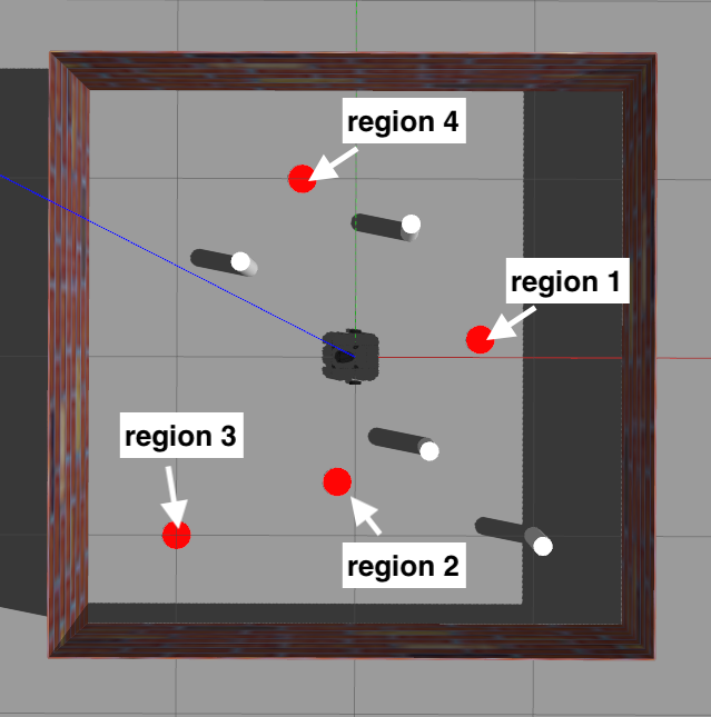
(a) Training Environment

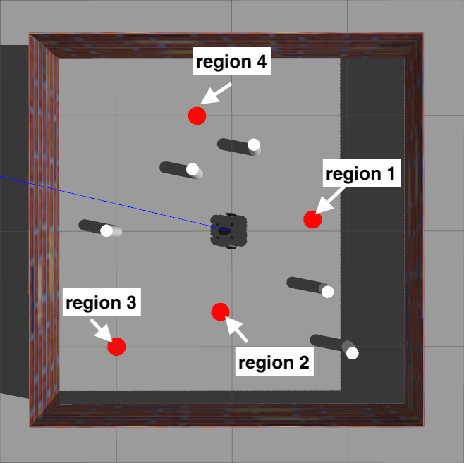
(b) Test Environment

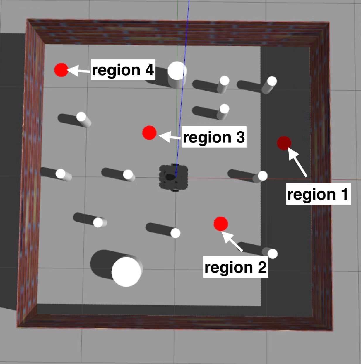
(c) Training Environment

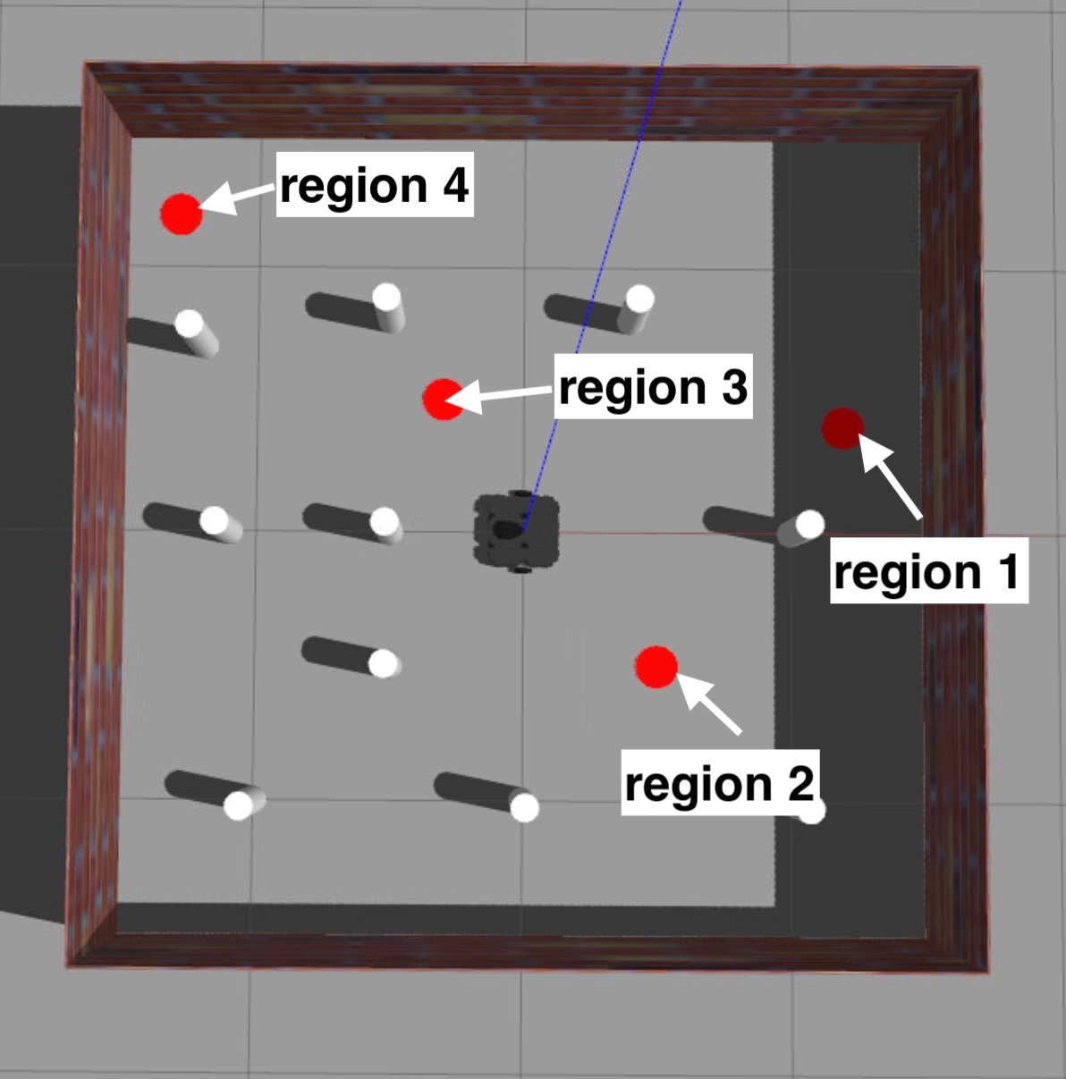
(d) Test Environment

Figure 1: Graphical illustration of the environments. Fig 1(a) and 1(b) show example environments for case studies I, III and IV; Fig 1(c) and 1(d) show example environments for case studies II.

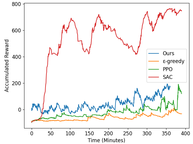
(a) Case Study I-(i)

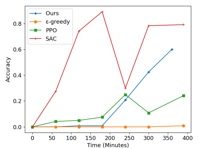
(b) Case Study I-(ii)

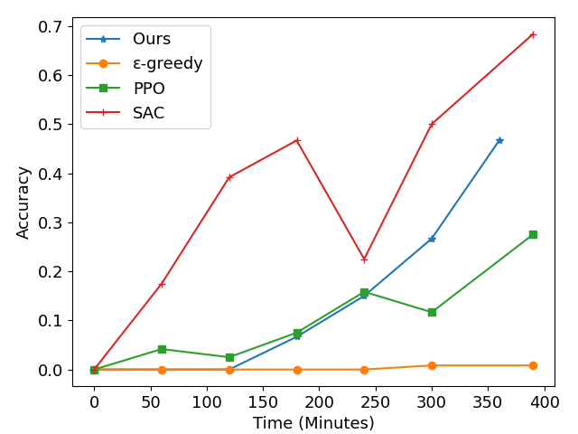
(c) Case Study I-(iii)

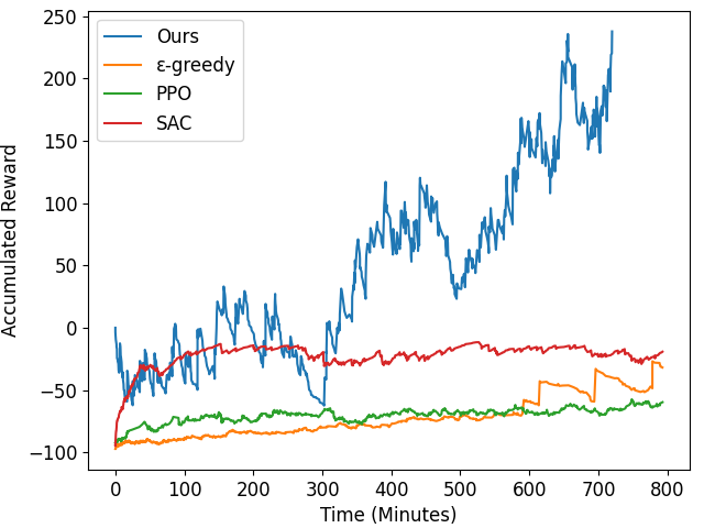
(d) Case Study II-(i)

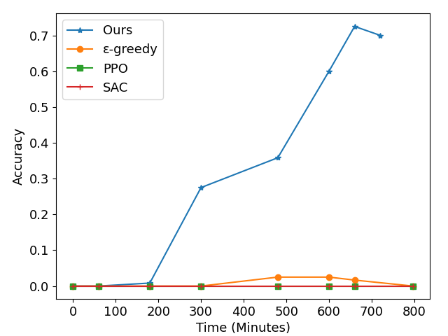
(e) Case Study II-(ii)

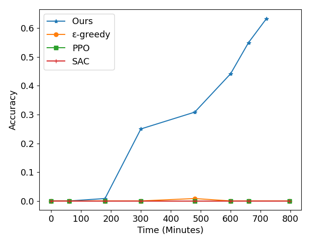
(f) Case Study II-(iii)

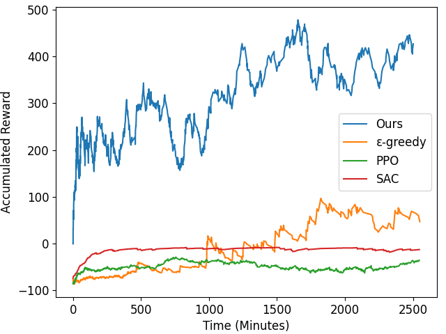
(g) Case Study III-(i)

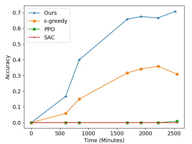
(h) Case Study III-(ii)

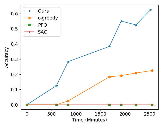
(i) Case Study III-(iii)

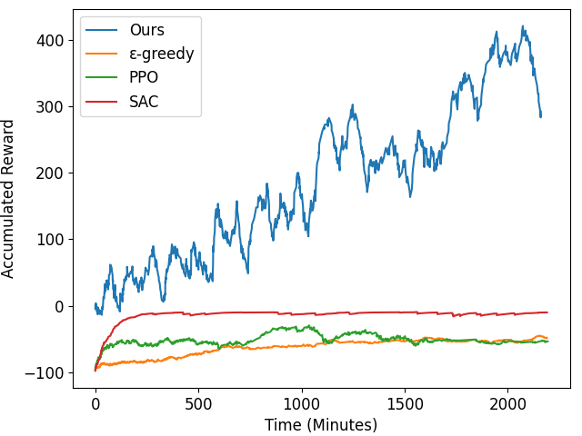
(j) Case Study IV-(i)

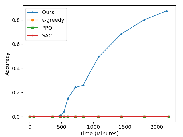
(k) Case Study IV-(ii)

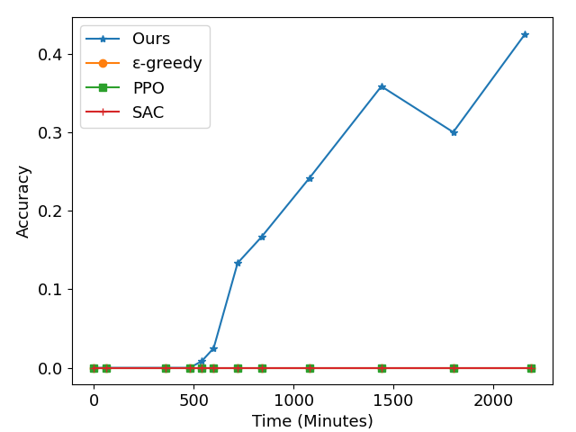
(l) Case Study IV-(iii)

Figure 2: Graphical Illustration of the evaluation metrics (i)-(iii) in each case study. Figs. (a), (d), (g), (j) (first column) showcase the evaluation metric (i) for Case study I-IV, respectively. Similarly, the figures in the second and third column illustrate the evaluation metrics (ii)-(iii), respectively, for each case study. In all figures, blue, orange, green, and red curves represent our method, standard DQN, PPO, and SAC, respectively.

Case Study I: First, we consider a simple navigation task, where the robot has to visit known regions ${r_{1}}$, ${r_{2}}$, and ${r_{3}}$ in any order while always avoiding unknown obstacles. This task can be captured by the LTL formula $\phi=\lozenge\pi^{r_{1}}\wedge\lozenge\pi^{r_{2}}\wedge\lozenge\pi^{r_{3}}\wedge\square\neg\pi^{W_{\text{obs}}}$ corresponding to a DRA with $9$ states and $1$ accepting pair. The time to train the NN $g$ is $T_{g}=0.5$ hour. For this task, we select $T_{\epsilon,\delta}=6$ hours. The return as well as the test-time accuracy in training and test environments are illustrated in Fig. 2(a), 2(b) and 2(c) respectively. SAC achieved the best performance across all metrics while our method outperformed both PPO and $\epsilon$-greedy method. As the training time increases, the test time accuracy of all methods tends to increase. Also, the test-time accuracy of all controllers demonstrates a decline ($\sim$10%) in unseen environments compared to the training set.

Case Study II: To illustrate how environmental complexity may impact sample efficiency, here, we consider the same LTL task as in Case Study I but over more complex environments. Specifically, the number of obstacles in the considered environments ranges from $10$ to $12$. The time required to train the NN $g$ is $T_{g}=1.28$ hour. For this task, we select $T_{\epsilon,\delta}=12$ hours. The performance of all methods based on the considered evaluation metrics is demonstrated in Fig. 2(d)-2(f). Unlike Case Study I, all the baselines - including SAC - struggle to gather non-negative rewards or develop a viable test-time policy due to the increased environmental complexity. In fact, the test-time accuracy of the controllers learned by the baselines, within the allotted training time, is almost $0\%$. To the contrary, our method has achieved a significantly higher test time accuracy in both training ($72.5\%$) and test environments ($63\%$) due to the proposed mission-driven exploration strategy.

Case Study III: Next, we consider a task requiring the robot to visit known regions ${r_{1}}$, ${r_{2}}$, ${r_{3}}$, ${r_{4}}$ in any order, as long as $r_{4}$ is visited only after $r_{1}$ is visited, and always avoid unknown obstacles. This task can be captured by the LTL formula $\phi=\lozenge\pi^{r_{1}}\wedge\lozenge\pi^{r_{4}}\wedge(\neg\pi^{r_{4}}{\mathcal{U}}\pi^{r_{1}})\wedge\lozenge\pi^{r_{2}}\wedge\lozenge\pi^{r_{3}}\wedge\square\neg\pi^{W_{\text{obs}}}$. This formula corresponds to a DRA with $13$ states and $1$ accepting pair. For this task, we have $T_{g}=0.5$ hours and we select $T_{\epsilon,\delta}=42$ hours. Note that this task is more complex than the previous one it involves a larger set of regions of interest that also need to be visited in a pre-specified order. The results are summarized in Figs. 2(g)-2(i). Observe that our method has achieved the best performance across all metrics. In fact, PPO and SAC have not managed to collect any positive rewards within the available training while standard DQN has started collecting non-negative rewards after approximately $1,000$ minutes of training. The accuracy of PPO, SAC, and DQN in test environments is $0\%$, $0\%$, $22.5\%$. Similar performance is attained in training environments. Unlike these baselines, our proposed method has already achieved a satisfactory test-time accuracy in training ($70.8\%$) and test ($62.5\%$) environments.

Case Study IV: Here we consider a long-horizon navigation task, where the robot has to visit ${r_{1}}$ and ${r_{4}}$ in this order while visiting ${r_{2}}$, ${r_{3}}$ infinitely often and avoiding obstacles ${\mathcal{W}}_{\text{obs}}$ all the time. This task can be captured by the LTL formula $\phi=\lozenge\pi^{r_{1}}\wedge\lozenge\pi^{r_{4}}\wedge(\neg\pi^{r_{4}}{\mathcal{U}}\pi^{r_{1}})\wedge\lozenge\square\pi^{r_{2}}\wedge\square\lozenge\pi^{r_{3}}\wedge\square\neg\pi^{{\mathcal{W}}_{\text{obs}}}$. This formula corresponds to a DRA with $10$ states and $1$ accepting pair. Notice that this task is more complex than the previous ones as it requires to visit certain regions repeatedly. Thus, we select $T_{\epsilon,\delta}=36$ hours. For this task, we have that $T_{g}=0.5$ hour. The performance of all algorithms is visualized in Figs. 2(j)-2(l). It is noteworthy that, due to the increased task complexity, all baselines are ineffective in collecting any non-negative rewards or learning a satisfactory policy throughout the entire training runtime. In fact, the test time accuracy of all baselines is $0\%$. However, our method manages to collect a significantly high return while achieving a test time accuracy of $88.3\%$ and $42.5\%$ in training and test environments, respectively.

V Conclusions & Future Work

We proposed a new sample-efficient deep RL algorithm for LTL-encoded tasks. Its sample efficiency relies on prioritizing exploration in the vicinity of task-related regions as supported by our comparative experiments. Our future work will focus on extending the proposed framework to high-dimensional state and action spaces and evaluating it on missions that go beyond navigation (e.g., locomotion tasks).

Appendix A Hardware Experiments

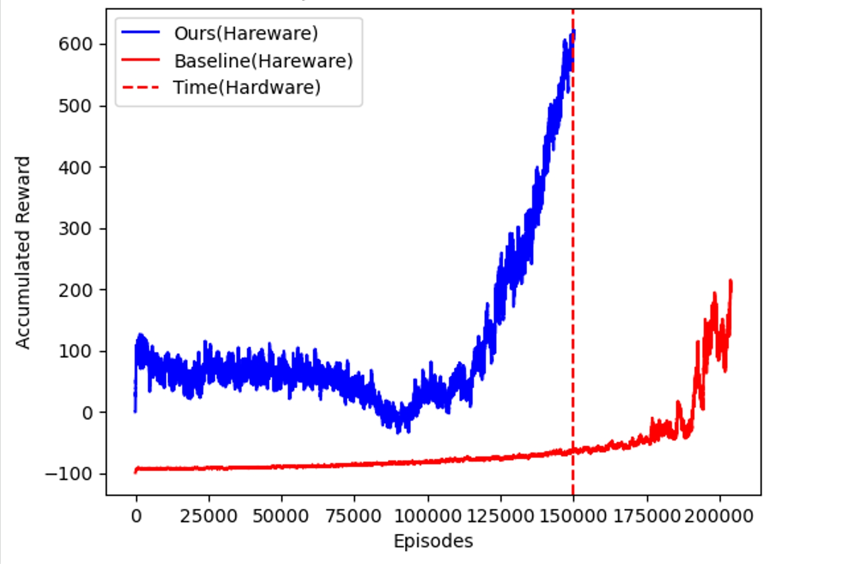
(a) Episodic returns

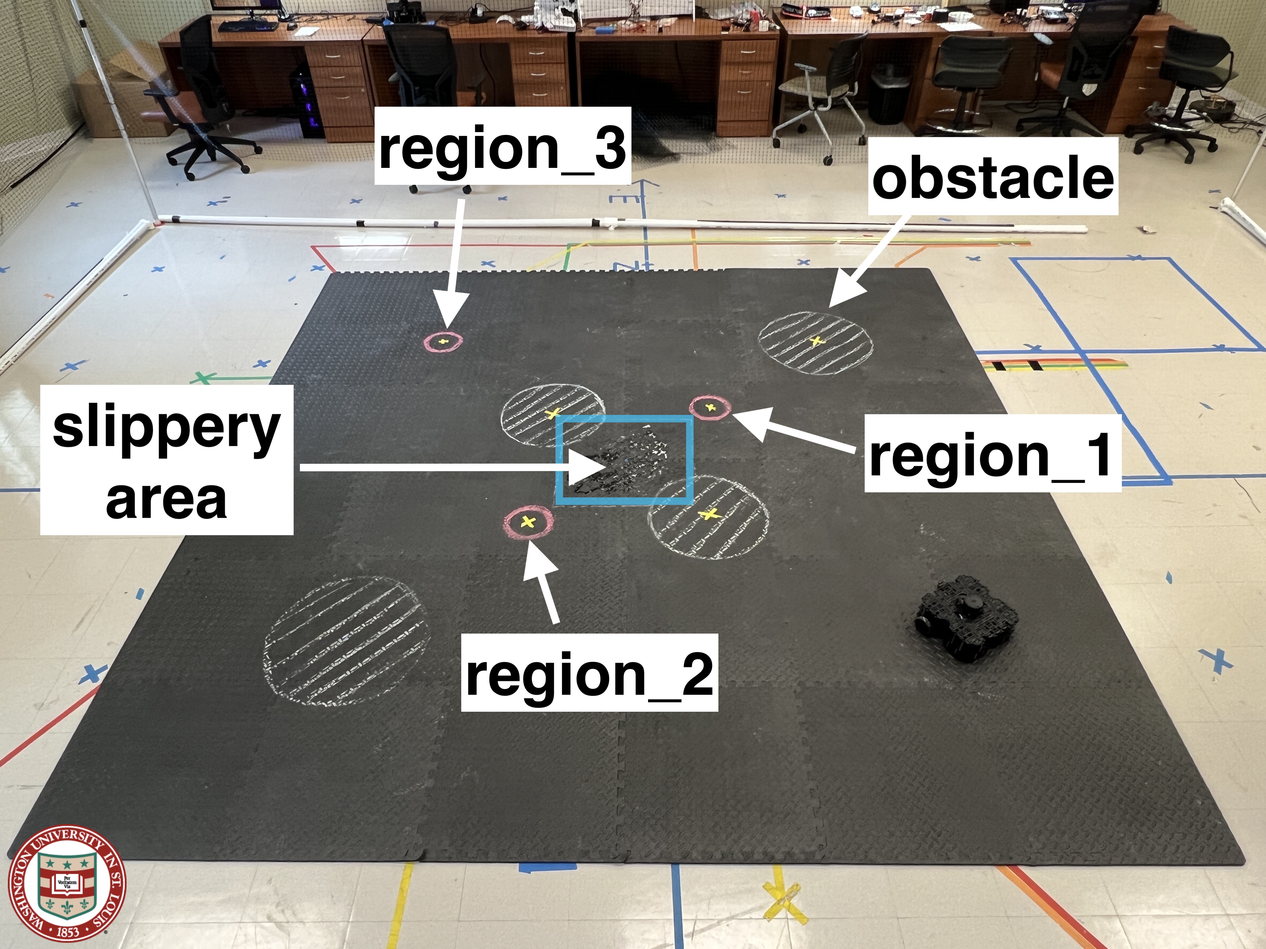
(b) Environment

Figure 3: Hardware experiments on ground robot navigation tasks.

In this section, we provide hardware experiments to demonstrate the performance of the proposed algorithms and how they may be affected by the sim2real gap. Hereafter, we consider a $3\text{m}\times 3\text{m}$ environment with $4$ obstacle-regions. A small area $x,y\in[-0.3,0.3]$ in the middle of the workspace is slippery due to spilled water. To model this, we define a state-dependent noise. Specifically, we model actuation noise as (i) $w_{t}^{u},w_{t}^{\omega}\sim\mathcal{N}(2e^{-3},1e^{-3})$ when the robot is outside the slippery area and (ii) $w_{t}^{u}\sim\mathcal{N}(2e^{-3},1e^{-3})$ and and $w_{t}^{\omega}\sim\mathcal{N}(2e^{-3},0.5)$ when the robot is in the slippery area. The average time to train a NN $g$ is $T_{g}=4$ hours. We apply Alg. 1 with $(\epsilon,\delta)-$greedy policy for $T_{\epsilon,\delta}=28$ hours. The comparative results are set up by following the same process as discussed in Section IV-B.

We consider a task captured by the following LTL formula: $\phi=\lozenge\pi^{r_{1}}\wedge\lozenge\pi^{r_{2}}\wedge(\neg\pi^{r_{2}}{\mathcal{U}}\pi^{r_{1}})\wedge\lozenge\pi^{r_{3}}\wedge\square\neg\pi^{{\mathcal{W}}_{\text{obs}}}$. In words, this task requires the robot to (i) eventually visit $r_{1}$; (ii) eventually visit $r_{2}$ but only after $r_{1}$ is visited; (iii) eventually visit $r_{3}$; and (iv) always avoid obstacles. This formula corresponds to a DRA with $7$ states and $1$ accepting pair. First, we learn control policies using the simulator discussed in Section IV-A using both $\epsilon-$ and $(\epsilon,\delta)$-greedy policy. The comparative results are summarized in Fig. 3(a). During training we considered a single training environment. Observe that our algorithm starts collecting positive rewards quite fast outperforming the baseline. Due to the task simplicity, the $\epsilon-$greedy policy managed to collect positive rewards within the first $200,000$ episodes.

In what follows, we evaluate the sim-to-real gap on a ground robot platform (Turtlebot 3 Waffle Pi). As a test environment, we consider the training one. Then, we sample $13$ initial robot states $x_{0}$ and we simulate the system trajectories using the simulator. The test-time accuracy, as evaluated in the simulator, of our policy is $92\%$ while the accuracy of the policy learned using uniform/random exploration is $38.5\%$. Notice that our method generates more reliable policies in the same amount of training time. We observe also that the learned policies avoid the slippery area even though it lies in the shortest path between $r_{1}$ and $r_{2}$ (see Fig. 3(b) and the supplemental video).

Next, we deploy the robot in an environment structured exactly as the training one; see Fig. 3(b). Then, we apply these policies on the ground robot using the same initial states as before. We observed that the test time accuracy dropped to $69.2\%$ and $23\%$ for our method and the baseline, respectively, even though the training and test environments are the same. This accuracy drop may be due to the reality gap, i.e., due to inaccurate modeling of the actuation noise and/or the system dynamics. For instance, in our simulations, we assume perfect state estimation while, in our experiments, the robot localizes itself using SLAM [38].

References

- [1] B. R. Kiran, I. Sobh, V. Talpaert, P. Mannion, A. A. Al Sallab, S. Yogamani, and P. Pérez, “Deep reinforcement learning for autonomous driving: A survey,” IEEE Transactions on Intelligent Transportation Systems, vol. 23, no. 6, pp. 4909–4926, 2021.
- [2] Y. F. Chen, M. Everett, M. Liu, and J. P. How, “Socially aware motion planning with deep reinforcement learning,” in 2017 IEEE/RSJ International Conference on Intelligent Robots and Systems (IROS). IEEE, 2017, pp. 1343–1350.
- [3] D. Dewey, “Reinforcement learning and the reward engineering principle,” in 2014 AAAI Spring Symposium Series, 2014.
- [4] C. Baier and J.-P. Katoen, Principles of model checking. MIT press Cambridge, 2008, vol. 26202649.
- [5] E. M. Hahn, M. Perez, S. Schewe, F. Somenzi, A. Trivedi, and D. Wojtczak, “Omega-regular objectives in model-free reinforcement learning,” TACAS, 2018.
- [6] Q. Gao, D. Hajinezhad, Y. Zhang, Y. Kantaros, and M. M. Zavlanos, “Reduced variance deep reinforcement learning with temporal logic specifications,” in 10th ACM/IEEE International Conference on Cyber-Physical Systems, 2019, pp. 237–248.
- [7] M. Hasanbeig, Y. Kantaros, A. Abate, D. Kroening, G. J. Pappas, and I. Lee, “Reinforcement learning for temporal logic control synthesis with probabilistic satisfaction guarantees,” in 58th IEEE Conference on Decision and Control (CDC), Nice, France, December 2019.
- [8] A. K. Bozkurt, Y. Wang, M. M. Zavlanos, and M. Pajic, “Control synthesis from linear temporal logic specifications using model-free reinforcement learning,” in 2020 IEEE International Conference on Robotics and Automation (ICRA). IEEE, 2020, pp. 10 349–10 355.
- [9] M. Cai, M. Hasanbeig, S. Xiao, A. Abate, and Z. Kan, “Modular deep reinforcement learning for continuous motion planning with temporal logic,” IEEE RA-L, vol. 6, no. 4, pp. 7973–7980, 2021.
- [10] C. Wang, Y. Li, S. L. Smith, and J. Liu, “Continuous motion planning with temporal logic specifications using deep neural networks,” arXiv preprint arXiv:2004.02610, 2020.
- [11] K. Jothimurugan, S. Bansal, O. Bastani, and R. Alur, “Compositional reinforcement learning from logical specifications,” Advances in Neural Information Processing Systems, vol. 34, 2021.
- [12] S. Bansal, “Specification-guided reinforcement learning,” in Static Analysis: 29th International Symposium, SAS, Auckland, New Zealand, December 5–7, 2022, Proceedings. Springer, pp. 3–9.
- [13] M. Hasanbeig, D. Kroening, and A. Abate, “LCRL: Certified policy synthesis via logically-constrained reinforcement learning,” in CONFEST. Springer, 2022, pp. 217–231.
- [14] R. T. Icarte, T. Q. Klassen, R. Valenzano, and S. A. McIlraith, “Reward machines: Exploiting reward function structure in reinforcement learning,” Journal of Artificial Intelligence Research, 2022.
- [15] M. Cai, M. Mann, Z. Serlin, K. Leahy, and C.-I. Vasile, “Learning minimally-violating continuous control for infeasible linear temporal logic specifications,” arXiv preprint arXiv:2210.01162, 2022.
- [16] A. Balakrishnan, S. Jaksic, E. Aguilar, D. Nickovic, and J. Deshmukh, “Model-free reinforcement learning for symbolic automata-encoded objectives,” in 25th ACM International Conference on Hybrid Systems: Computation and Control, 2022, pp. 1–2.
- [17] D. Pathak, P. Agrawal, A. A. Efros, and T. Darrell, “Curiosity-driven exploration by self-supervised prediction,” in International conference on machine learning. PMLR, 2017, pp. 2778–2787.
- [18] H. Hasanbeig, N. Yogananda Jeppu, A. Abate, T. Melham, and D. Kroening, “DeepSynth: Program synthesis for automatic task segmentation in deep reinforcement learning,” in AAAI. Association for the Advancement of Artificial Intelligence, 2021.
- [19] H. Zhang, H. Wang, and Z. Kan, “Exploiting transformer in sparse reward reinforcement learning for interpretable temporal logic motion planning,” IEEE Robotics and Automation Letters, 2023.
- [20] M. Cai, E. Aasi, C. Belta, and C.-I. Vasile, “Overcoming exploration: Deep reinforcement learning for continuous control in cluttered environments from temporal logic specifications,” IEEE Robotics and Automation Letters, vol. 8, no. 4, pp. 2158–2165, 2023.
- [21] Y. Zhai, C. Baek, Z. Zhou, J. Jiao, and Y. Ma, “Computational benefits of intermediate rewards for goal-reaching policy learning,” Journal of Artificial Intelligence Research, vol. 73, pp. 847–896, 2022.
- [22] J. Fu and U. Topcu, “Probably approximately correct mdp learning and control with temporal logic constraints,” arXiv preprint arXiv:1404.7073, 2014.
- [23] T. Brázdil, K. Chatterjee, M. Chmelik, V. Forejt, J. Křetínskỳ, M. Kwiatkowska, D. Parker, and M. Ujma, “Verification of Markov decision processes using learning algorithms,” in ATVA. Springer, 2014, pp. 98–114.
- [24] M. Perez, F. Somenzi, and A. Trivedi, “A PAC learning algorithm for LTL and omega-regular objectives in MDPs,” arXiv preprint arXiv:2310.12248, 2023.
- [25] V. Mnih, K. Kavukcuoglu, D. Silver, A. Graves, I. Antonoglou, D. Wierstra, and M. Riedmiller, “Playing Atari with deep reinforcement learning,” arXiv preprint arXiv:1312.5602, 2013.
- [26] H. Van Hasselt, A. Guez, and D. Silver, “Deep reinforcement learning with double Q-learning,” in Proceedings of the AAAI conference on artificial intelligence, vol. 30, no. 1, 2016.
- [27] M. Hessel, J. Modayil, H. Van Hasselt, T. Schaul, G. Ostrovski, W. Dabney, D. Horgan, B. Piot, M. Azar, and D. Silver, “Rainbow: Combining improvements in deep reinforcement learning,” in Proceedings of the AAAI conference on artificial intelligence, 2018.
- [28] Y. Kantaros, “Accelerated reinforcement learning for temporal logic control objectives,” in IEEE/RSJ International Conference on Intelligent Robots and Systems, Kyoto, Japan, October 2022.
- [29] Y. Kantaros, S. Kalluraya, Q. Jin, and G. J. Pappas, “Perception-based temporal logic planning in uncertain semantic maps,” IEEE Transactions on Robotics, vol. 38, no. 4, pp. 2536–2556, 2022.
- [30] K. Leahy, D. Zhou, C.-I. Vasile, K. Oikonomopoulos, M. Schwager, and C. Belta, “Persistent surveillance for unmanned aerial vehicles subject to charging and temporal logic constraints,” Autonomous Robots, vol. 40, no. 8, pp. 1363–1378, 2016.
- [31] M. Guo and M. M. Zavlanos, “Distributed data gathering with buffer constraints and intermittent communication,” in IEEE International Conference on Robotics and Automation (ICRA), 2017.
- [32] Y. Kantaros and M. M. Zavlanos, “Distributed intermittent connectivity control of mobile robot networks,” IEEE Transactions on Automatic Control, vol. 62, no. 7, pp. 3109–3121, 2016.
- [33] A. Faust, K. Oslund, O. Ramirez, A. Francis, L. Tapia, M. Fiser, and J. Davidson, “PRM-RL: Long-range robotic navigation tasks by combining reinforcement learning and sampling-based planning,” in IEEE ICRA, 2018, pp. 5113–5120.
- [34] Y. Kantaros and M. M. Zavlanos, “STyLuS*: A temporal logic optimal control synthesis algorithm for large-scale multi-robot systems,” The International Journal of Robotics Research, vol. 39, no. 7, pp. 812–836, 2020.
- [35] Y. Kantaros, B. Schlotfeldt, N. Atanasov, and G. J. Pappas, “Sampling-based planning for non-myopic multi-robot information gathering,” Autonomous Robots, vol. 45, no. 7, pp. 1029–1046, 2021.
- [36] J. Schulman, F. Wolski, P. Dhariwal, A. Radford, and O. Klimov, “Proximal policy optimization algorithms,” arXiv preprint arXiv:1707.06347, 2017.
- [37] T. Haarnoja, A. Zhou, P. Abbeel, and S. Levine, “Soft actor-critic: Off-policy maximum entropy deep reinforcement learning with a stochastic actor,” in International conference on machine learning. PMLR, 2018, pp. 1861–1870.
- [38] G. Grisetti, C. Stachniss, and W. Burgard, “Improved techniques for grid mapping with rao-blackwellized particle filters,” IEEE transactions on Robotics, vol. 23, no. 1, pp. 34–46, 2007.