Stability estimates of Nyström discretizations of Helmholtz decomposition boundary integral equation formulations for the solution of Navier scattering problems in two dimensions with Dirichlet boundary conditions

Abstract

Helmholtz decompositions of elastic fields is a common approach for the solution of Navier scattering problems. Used in the context of Boundary Integral Equations (BIE), this approach affords solutions of Navier problems via the simpler Helmholtz boundary integral operators (BIOs). Approximations of Helmholtz Dirichlet-to-Neumann (DtN) can be employed within a regularizing combined field strategy to deliver BIE formulations of the second kind for the solution of Navier scattering problems in two dimensions with Dirichlet boundary conditions, at least in the case of smooth boundaries. Unlike the case of scattering and transmission Helmholtz problems, the approximations of the DtN maps we use in the Helmholtz decomposition BIE in the Navier case require incorporation of lower order terms in their pseudodifferential asymptotic expansions. The presence of these lower order terms in the Navier regularized BIE formulations complicates the stability analysis of their Nyström discretizations in the framework of global trigonometric interpolation and the Kussmaul-Martensen kernel singularity splitting strategy. The main difficulty stems from compositions of pseudodifferential operators of opposite orders, whose Nyström discretization must be performed with care via pseudodifferential expansions beyond the principal symbol. The error analysis is significantly simpler in the case of arclength boundary parametrizations and considerably more involved in the case of general smooth parametrizations which are typically encountered in the description of one dimensional closed curves.
Keywords: Time-harmonic Navier scattering problems, Helmholtz decomposition, boundary integral equations, pseudodifferential calculus, Nyström discretizations, regularizing operators.

AMS subject classifications: 65N38, 35J05, 65T40, 65F08

1 Introduction

Elastic waves in homogeneous media, that is solutions of the time harmonic Navier equations, can be expressed via Helmholtz decompositions as linear superpositions of P-waves and S-waves, which are in turn solutions of Helmholtz equations with different wavenumbers related to the Lamé constants of the medium in which they propagate. The enforcement of Dirichlet boundary conditions in this approach leads to coupled boundary conditions for the pressure and the shear waves featuring normal and tangential derivatives on the boundary of the scatterer. This simple observation affords the possibility to use Helmholtz potentials corresponding to the pressure and shear wave numbers and their related boundary integral operators (BIOs) to solve time harmonic Navier scattering problems in homogeneous media. This approach has to be contrasted to the classical BIE approaches based on Navier Green’s function potentials [16, 14, 15, 17, 22, 11, 19].

The combined field approach [7], which is the method of choice to deliver robust BIE formulations for Helmholtz scattering problems at any frequencies, leads in this context to systems of BIE of the first kind (pseudodifferential operators of order one) owing to the presence of Helmholtz hypersingular BIOs. To compound the difficulty, the principal symbols (in the pseudodifferential operator sense) of these combined field formulations are defective matrix operators [21, 20]. The regularized combined field methodology [3] relies on approximations of Dirichlet to Neumann (DtN) operators to construct intrinsically well conditioned boundary integral equations, which, in the case of smooth boundaries, are always of the second kind. This strategy was successfully applied to the design of well conditioned Navier BIE by incorporating suitable approximations of Navier DtN operators [9, 10, 19, 8]. The Helmholtz decomposition approach bypasses the need to construct the latter, as only Helmholtz DtN are required [20]. However, in order to mitigate the aforementioned defective property, the DtN approximations require incorporating lower order terms in the pseudodifferential asymptotic expansion of DtN operators [20]. Leveraging arclength parametrization, the pseusodifferential calculus beyond the principal symbol can be carried out within the framework of periodic Fourier multipliers. This calculus gets more delicate in the case of arbitrary parametrizations, and we present in this paper such a generalization that is invariant of the parametrization.

We introduce and analyze stable Nyström discretizations of the regularized BIE for the solutions of Navier scattering problems in the Helmholtz decomposition framework. The stable Nyström discretization of the composition of pseudodifferential operators of opposite orders that typically feature in regularized BIE formulations must be done with care [6]. The stable approach to deal with such compositions in the global trigonometric framework to isolate the principal parts of the pseudodifferential operators of opposite orders and effect their composition explicitly via Fourier multiplication calculus. Once the principal parts were dealt with, the composition of pseudodifferential operators of negative orders is benign, and can be realized by simple multiplication of Nyström discretization matrices. Our Nyström approach relies on Kussmaul-Martensen kernel logarithmic splittings [27, 28], which leads naturally to constructing asymptotic pseudodifferential expansions of the Helmholtz BIOs and therefore to carrying out operator compositions per the prescriptions above. This approach was adopted and developed in the 80s of the previous century by R. Kress and collaborators to provide a full discretization of the four layer operators for Helmholtz equations for which a rigorous proof of stability and convergence was given in the Sobolev framework cf [25, 24] (see also [5, 18]). For Helmholtz equation, the resulting scheme is known to be superalgebraically convergent, that is, faster than any negative power of the number of points used in this discretization, provided that the exact solution is smooth. We stress that same convergence order is stated in this work for this more complex equation.

The error analysis of the Nyström discretizations of the regularized BIE considered in this paper is conducted along the guidelines above, with extra complications that are inevitable to the presence of several terms in the pseudodifferential expansions of some of the key BIOs in our formulations, including the regularizing operators and the DtN approximations themselves. We chose to present the analysis both in the simpler arclength parametrization framework, as well as in the more complicated, yet more realistic case of general smooth parametrization of closed boundary curves. The use of smooth but non-arc length parametrizations is often necessary. In practice, it is not difficult to compute numerically sufficiently accurate approximations of the arc parametrization, even for rather complex geometries. However, such parametrizations result in an approximately uniform distribution of points along the curve, failing to distinguish between regions of rapid or slow variation in the curve (i.e., regions of high or low curvature). Since some of the most popular numerical schemes, such as the superalgebraically convergent Kress-Nyström discretization of the Helmholtz boundary integral operators we consider in this paper, use second and even third derivatives of the parametrization in the definition, this results in poor performance and/or very high sensitivity to round-off errors arising in the splitting of the kernels of the integral operators into smooth and singular parts. We provide evidence of these phenomena in the numerical experiments section.

We also believe that the design of other discretizations -such as those based on Petrov-Galerkin, Collocation or Qualocation spline based methods (see [2, 33, 30, 31] and references therein) or even deltaBEM schemes [13, 32]- and their mathematical analysis, are also possible up to some extent. However, in addition to the high order the Nyström method enjoys, there is a notable feature that makes the method considered and fully analysed here attractive: Both the regularizer and the approximation we propose for the Dirichlet-to-Neumann operator used in the pressure and shear wave representation formula are diagonal Fourier operators (i.e., convolution operators) for arc-length parametrizations of the curve which favours a simple integration with the solver. For general parametrizations this is only true for their principal parts, which is still advantageous. On the other hand, we are confident that Nyström discretization can also be analysed for the Neumann problem -the integral equation is in this case of order 1 (i.e. it behaves as a derivative)- by employing similar tools as those we have developed in this paper in a more complex and/or technical analysis. Numerical experiments support clearly this conjecture (see [20]).

The paper is organized as follows: in Section 2 we introduce the boundary value problem for Navier equations in two dimensions and we present the Helmholtz decomposition approach and a first boundary integral formulation for this problem. In Section 3 we rewrite the boundary integral equations as periodic operator equations by means of arc-length parametrizations of the boundary of the Navier problem domain. The required regularizer is then introduced and the well-posedness of the equation is stated. In Section 4 we introduce the Nyström method and prove stability and superalgebraically convergence for this equation; in Section 5 we construct the regularizing operators for general parametrizations, we extend the Nyström discretization for the regularized formulations and show that stability and superalgebraically convergence is preserved. Finally, we present in Section 6 a few numerical experiments to illustrate the second kind nature of the regularized formulations, the superalgebraically convergence proved in this paper as well as comparisons between the iterative behavior of Nyström solvers for both types of parametrizations considered in this paper.

2 Navier equations and boundary element method

2.1 Boundary value problem and Helmholtz decomposition

For any vector function ${\bf u}=(u_{1},u_{2})^{\top}:\mathbb{R}^{2}\to\mathbb{R}^{2}$ (vectors in this paper will be always regarded as column vectors) the strain tensor in a linear isotropic and homogeneous elastic medium with Lamé constants $\lambda$ and $\mu$ is defined as

$$\bm{\epsilon}({\bf u}):=\frac{1}{2}(\nabla{\bf u}+(\nabla{\bf u})^{\top})=\begin{bmatrix}\partial_{x_{1}}u_{1}&\tfrac{1}{2}\left(\partial_{x_{1}}u_{2}+\partial_{x_{2}}u_{1}\right)\\ \tfrac{1}{2}\left(\partial_{x_{1}}u_{2}+\partial_{x_{2}}u_{1}\right)&\partial_{x_{2}}u_{2}\end{bmatrix}.$$

The stress tensor is then given by

$$\bm{\sigma}({\bf u}):=2\mu\bm{\epsilon}({\bf u})+\lambda(\operatorname{div}{\bf u})I_{2}$$

where $I_{2}$ is the identity matrix of order 2 and the Lamé coefficients $\lambda$ are assumed to satisfy $\lambda,\ \lambda+2\mu>0$. For $\Omega$ a smooth bounded domain with boundary $\Gamma$, the exterior Dirichlet problem for the time-harmonic elastic wave (Navier) equation is

$$\left|\begin{array}[]{l}\operatorname{div}\bm{\sigma}({\bf u})+\omega^{2}{\bf u}=0,\quad\text{in }\Omega^{+}:=\mathbb{R}^{2}\setminus{\color[rgb]{1,0,0}\Omega},\\ \gamma_{\Gamma}{\bf u}=-{\bf u}^{\rm inc},\\ \text{+Kupradze radiation condition}\end{array}\right.$$ (2.1)

where the frequency $\omega\in\mathbb{R}^{+}$ and the divergence operator ${\rm div}$ is applied row-wise. Here ${\bf u}^{\rm inc}$ is a solution of the Navier equation in a neighborhood of $\overline{\Omega}$, typically in $\mathbb{R}^{2}$, although point source elastic waves are also supported.

The Kupradze radiation condition at infinity [1, 26] can be described as follows: if

$$\mathbf{u}_{p}:=-\frac{1}{k_{p}^{2}}\nabla\operatorname{div}\mathbf{u},\quad\mathbf{u}_{s}:=\mathbf{u}-\mathbf{u}_{p}=\operatorname{\overrightarrow{\mathrm{curl}}}{\rm{curl}\ {\bf u}}$$ (2.2)

($\operatorname{\overrightarrow{\mathrm{curl}}}\varphi:=(\partial_{x_{2}}\varphi,-\partial_{x_{1}}\varphi)$, $\operatorname{curl}{\bf u}:=\partial_{x_{2}}u_{1}-\partial_{x_{1}}u_{2}$ are respectively the vector and scalar curl, or rotational, operator) with

$$k_{p}^{2}:=\frac{\omega^{2}}{\lambda+2\mu},\quad k_{s}^{2}:=\frac{\omega^{2}}{\mu}$$ (2.3)

the associated the pressure and stress wave-numbers wave-numbers, then

$$\frac{\partial\mathbf{u}_{p}}{\partial\widehat{\bm{x}}}(\bm{x})-ik_{p}\mathbf{u}_{p}(\bm{x}),\quad\frac{\partial\mathbf{u}_{s}}{\partial\widehat{\bm{x}}}(\bm{x})-ik_{s}\mathbf{u}_{s}(\bm{x})=o\left(|\bm{x}|^{-1/2}\right),\quad\widehat{\bm{x}}:=\frac{1}{|\bm{x}|}\bm{x}.$$

In view of (2.2), a common approach to the solution of Navier equations is to look for the fields ${\bf u}$ in the form

$${\bf u}=\nabla u_{p}+\operatorname{\overrightarrow{\mathrm{curl}}}{u_{s}}$$ (2.4)

where $u_{p}$ and $u_{s}$ are respectively solutions of the Helmholtz equations in $\Omega^{+}$ with wave-numbers $k_{p}$ and $k_{s}$ satisfying the Sommerfeld radiation condition at infinity which is in itself a simple consequence of the Kupradze radiation condition. Specifically, the scalar fields in the Helmholtz decomposition are solutions of the following Helmholtz problems

$$\left|\begin{array}[]{ll}\Delta u_{p}+k_{p}^{2}=0,\quad\text{in }\Omega^{+}\\ \partial_{\widehat{\bm{x}}}u_{p}-ik_{p}u_{p}=o(|\bm{x}|^{-1/2}),\quad\text{as }|{\bm{x}}|\to\infty\end{array}\right.\quad\left|\begin{array}[]{ll}\Delta u_{s}+k_{s}^{2}=0,\quad\text{in }\Omega^{+}\\ \partial_{\widehat{\bm{x}}}u_{s}-ik_{s}u_{s}=o(|\bm{x}|^{-1/2}),\quad\text{as }|{\bm{x}}|\to\infty.\end{array}\right.$$ (2.5)

If $\bm{n}$ denotes the outward unit normal vector to $\Gamma$, $\bm{t}$, the positively (counterclockwise) oriented tangent field given by

$$\bm{t}=-{\rm Q}\bm{n},\quad{\rm Q}:=\begin{bmatrix}0&1\\ -1&0\end{bmatrix}$$ (2.6)

which satisfy

$$\nabla{\bf u}_{p}\cdot\bm{n} =\partial_{\bm{n}}u_{p}\quad \nabla{\bf u}_{p}\cdot\bm{t} =\partial_{\bm{t}}u_{p}$$

$$\operatorname{\overrightarrow{\mathrm{curl}}}{\bf u}_{s}\cdot\bm{n} =\partial_{\bm{t}}u_{s}\quad \operatorname{\overrightarrow{\mathrm{curl}}}{\bf u}_{s}\cdot\bm{t} =-\partial_{\bm{n}}u_{s}$$

($\partial_{\bm{n}}$ and $\partial_{\bm{t}}$ are then the exterior normal and the positively oriented tangent derivative), the Dirichlet condition in problem (2.1) leads to the following boundary conditions on $\Gamma$ for $u_{p}$ and $u_{s}$:

$$\begin{array}[]{rcll}\partial_{\bm{n}}u_{p}+\partial_{\bm{t}}u_{s}&=&-{\bf u}^{\rm inc}\cdot\bm{n},&{\rm on}\ \Gamma,\\ \partial_{\bm{t}}u_{p}-\partial_{\bm{n}}u_{s}&=&-{\bf u}^{\rm inc}\cdot\bm{t},&{\rm on}\ \Gamma.\end{array}$$ (2.7)

The reformulation of the Navier scattering problem with Dirichlet boundary conditions in the Helmholtz decomposition framework is readily amenable to boundary integral formulations, as we will explain in what follows.

Remark 2.1

Throughout this article we will assume that $\Gamma$, the boundary of the domain $\Omega^{+}$, is of length $2\pi$. The general case can be reduced to this particular scenario by replacing the wawenumber(s) $k$, and the complexifications $\widetilde{k}$ we will introduce later, by $Lk/(2\pi)$, its characteristic length, and $L\widetilde{k}/(2\pi)$, where $L$ is the length of the curve.

2.2 Helmholtz BIOs

For a given wave-number $k>0$ and a functional density $\varphi_{\Gamma}$ on the boundary $\Gamma$ we define the Helmholtz single and double layer potentials in the form

$$\operatorname{SL}_{k,\Gamma}[\varphi_{\Gamma}]({\bm{x}}):=\int_{\Gamma}\phi_{k}({\bm{x}}-{\bm{y}})\varphi_{\Gamma}({\bm{y}}){{\rm d}{\bm{y}}},\quad\operatorname{DL}_{k,\Gamma}[\varphi_{\Gamma}]({\bm{x}}):=\int_{\Gamma}\frac{\partial\phi_{k}({\bm{x}}-{\bm{y}})}{\partial\bm{n}({\bm{y}})}\varphi_{\Gamma}({\bm{y}}){{\rm d}{\bm{y}}},\ {\bm{x}}\in\mathbb{R}^{2}\setminus\Gamma$$

with

$$\phi_{k}({\bm{x}})=\frac{i}{4}H_{0}^{(1)}(k|{\bm{x}}|)$$

the fundamental solution of the Helmholtz equation ($H_{0}^{(1)}$ is then the Hankel function of first kind and order zero).

The four BIOs of the Calderón’s calculus associated with the Helmholtz equation are defined by applying the exterior/interior Dirichlet and Neumann traces on $\Gamma$ (denoted in what follows by $\gamma_{\Gamma}^{+}/\gamma_{\Gamma}^{-}$ and $\partial_{\bm{n}}^{+}/\partial_{\bm{n}}^{-}$ respectively) to the Helmholtz single and double layer potentials cf. [23, 29, 31]. Specifically,

$$\gamma_{\Gamma}^{\pm}\operatorname{SL}_{k,\Gamma}\varphi_{\Gamma} =\operatorname{V}_{k,\Gamma}\varphi_{\Gamma},\quad \partial_{\bm{n}}^{\pm}\operatorname{SL}_{k,\Gamma}\varphi_{\Gamma} =\mp\frac{1}{2}\varphi_{\Gamma}+\operatorname{K}_{k,\Gamma}^{\top}\varphi_{\Gamma},$$ (2.8)

$$\gamma_{\Gamma}^{\pm}\operatorname{DL}_{k,\Gamma}\varphi_{\Gamma} =\pm\frac{1}{2}\varphi_{\Gamma}+\operatorname{K}_{k,\Gamma}\varphi_{\Gamma},\quad \partial_{\bm{n}}^{\pm}\operatorname{DL}_{k,\Gamma}\varphi_{\Gamma} =\operatorname{W}_{k,\Gamma}\varphi_{\Gamma}$$

where, for ${\bm{x}}\in\Gamma$,

$$(\operatorname{V}_{k,\Gamma}\varphi_{\Gamma})({\bm{x}}) := \int_{\Gamma}\phi_{k}({\bm{x}}-{\bm{y}})\varphi_{\Gamma}({\bm{y}}){{\rm d}{\bm{y}}},$$ (2.9)

$$(\operatorname{K}_{k,\Gamma}\varphi_{\Gamma})({\bm{x}}) := \int_{\Gamma}\frac{\partial\phi_{k}({\bm{x}}-{\bm{y}})}{\partial\bm{n}({\bm{y}})}\varphi_{\Gamma}({\bm{y}}){{\rm d}{\bm{y}}},$$ (2.10)

$$(\operatorname{K}_{k,\Gamma}^{\top}\varphi_{\Gamma})({\bm{x}}) := \int_{\Gamma}\frac{\partial\phi_{k}({\bm{x}}-{\bm{y}})}{\partial\bm{n}({\bm{x}})}\varphi_{\Gamma}({\bm{y}}){{\rm d}{\bm{y}}},$$ (2.11)

$$(\operatorname{W}_{k,\Gamma}\varphi_{\Gamma})({\bm{x}}) := \mathrm{f.p.}\int_{\Gamma}\frac{\partial^{2}\phi_{k}({\bm{x}}-{\bm{y}})}{\partial\bm{n}({\bm{x}})\,\partial\bm{n}({\bm{y}})}\varphi_{\Gamma}({\bm{y}}){{\rm d}{\bm{y}}}$$ (2.12)

$$= \partial_{\bm{t}({\bm{x}})}\operatorname{V}_{k,\Gamma}[\partial_{\bm{t}}\varphi_{\Gamma}]({\bm{x}})-k^{2}\bm{t}({{\bm{x}}})\cdot(\operatorname{V}_{k,\Gamma}[\bm{t}\varphi_{\Gamma}])({{\bm{x}}})$$

are respectively the single layer, double layer, adjoint double and hypersingular operator. In the latter operator, “f.p.” stands for finite part since the kernel of the operator is strongly singular. However, as noted, the hypersingular operator can also be written in terms of the single-layer operator and the tangent derivative $\partial_{\bm{t}}$ operator, an alternative expression which is sometimes referred to as Maue’s formula. The following not-so-well-known identities:

$$\partial_{\bm{t}({\bm{x}})}(\operatorname{SL}_{k,\Gamma}\varphi_{\Gamma})({\bm{x}}) = (\partial_{\bm{t}}\operatorname{V}_{k,\Gamma}\varphi_{\Gamma})({\bm{x}}),$$ (2.13)

$$\partial_{\bm{t}({\bm{x}})}(\operatorname{DL}_{k,\Gamma}\varphi_{\Gamma})({\bm{x}}) = \frac{1}{2}\partial_{\bm{t}}\varphi({\bm{x}})+k^{2}(\operatorname{V}_{k,\Gamma}(\bm{n}\varphi_{\Gamma}))({\bm{x}})\cdot\bm{t}({\bm{x}})-(\operatorname{K}^{\top}\partial_{\bm{t}}\varphi)({\bm{x}}),$$ (2.14)

again with ${\bm{x}}\in\Gamma$, will be used in the formulation of the method. We refer the reader to [20, Th. 3.5] for a proof.

Remark 2.2

From now on we will denote the layer operators and potentials associated to the Helmholtz equation with a generic wave-number $k$ with the subscript “$k$”. When we want to refer to $k_{p}$ or $k_{s}$, the pressure and strain wave-numbers associated to the Navier equation, we will use simply $p$ and $s$ for lighten the notation.

We propose then a solution of (2.4) in the form of a combined potential formulation for $u_{p}$ and $u_{s}$:

$$u_{p} ={\operatorname{DL}}_{p,\Gamma}\varphi_{p,\Gamma}-{\operatorname{SL}}_{p,\Gamma}\mathrm{Y}_{p,\Gamma}\varphi_{p,\Gamma},\quad$$ (2.15)

$$u_{s} ={\operatorname{DL}}_{s,\Gamma}\varphi_{p,\Gamma}-{\operatorname{SL}}_{s,\Gamma}\mathrm{Y}_{s,\Gamma}\varphi_{s,\Gamma},$$

in terms of densities $\varphi_{p,\Gamma},\ \varphi_{s,\Gamma}$. Here $\mathrm{Y}_{p,\Gamma}$ and $\mathrm{Y}_{s,\Gamma}$ are suitable approximations, which will be described precisely below, of the Dirichlet-to-Neumann operators $\mathcal{Y}_{p,\Gamma}$ and $\mathcal{Y}_{s,\Gamma}$ corresponding to exterior Helmholtz problems for $k_{p}$ and $k_{s}$ respectively. By construction, $u_{p}$ and $u_{s}$ are solutions of the Helmholtz equations satisfying the radiation (Sommerfeld) conditions at infinity. It is worth noting that with the use of such operators, the equation (2.15) resembles the representation formula of the exterior solutions of the Helmholtz equation in terms of the Dirichlet and Neumann data:

$$u_{k}={\operatorname{DL}}_{k,\Gamma}\gamma_{\Gamma}u_{k}-{\operatorname{SL}}_{p,\Gamma}\partial_{\bm{n}}u_{k}.$$

By imposing the Dirichlet conditions in the $(\bm{n},\bm{t})$ frame on $\Gamma$, and making use of the identities (2.8)–(2.14), the combined field approach leads to the following system of BIE for the densities $\varphi_{p,\Gamma}$ and $\varphi_{s,\Gamma}$

$$\mathcal{A}_{\rm comb,\Gamma}\begin{bmatrix}\varphi_{p,\Gamma}\\ \varphi_{s,\Gamma}\end{bmatrix}=\begin{bmatrix}f_{\bm{n},\Gamma}\\ f_{\bm{t},\Gamma}\end{bmatrix},\quad f_{\bm{n},\Gamma}=-\gamma_{\Gamma}{\bf u}^{\rm inc}\cdot\bm{n},\ f_{\bm{t},\Gamma}=-\gamma_{\Gamma}{\bf u}^{\rm inc}\cdot\bm{t}$$

where

$$\mathcal{A}_{\rm comb,\Gamma}:=\mathcal{A}_{\rm DL,\Gamma}-\mathcal{A}_{\rm SL,\Gamma}\begin{bmatrix}\mathrm{Y}_{p,\Gamma}&\\ &\mathrm{Y}_{s,\Gamma}\end{bmatrix}$$ (2.16)

with

$$\mathcal{A}_{\rm DL,\Gamma} := \begin{bmatrix}\operatorname{W}_{p,\Gamma}&\frac{1}{2}\partial_{\bm{t}}+k_{s}^{2}\bm{t}\cdot\operatorname{V}_{s,\Gamma}[\bm{n}\,\cdot\,]-\operatorname{K}_{s,\Gamma}^{\top}\partial_{\bm{t}}\\ \frac{1}{2}\partial_{\bm{t}}+k_{p}^{2}\bm{t}\cdot\operatorname{V}_{p,\Gamma}[\bm{n}\,\cdot\,]-\operatorname{K}_{p,\Gamma}^{\top}\partial_{\bm{t}}&-\operatorname{W}_{s,\Gamma}\end{bmatrix}$$ (2.17)

$$\mathcal{A}_{\rm SL,\Gamma} := \begin{bmatrix}-\frac{1}{2}\operatorname{I}+\operatorname{K}_{p,\Gamma}^{\top}&\partial_{\bm{t}}\operatorname{V}_{s,\Gamma}\\ \partial_{\bm{t}}\operatorname{V}_{p,\Gamma}&\frac{1}{2}\operatorname{I}-\operatorname{K}_{s,\Gamma}^{\top}\end{bmatrix}.$$ (2.18)

Equation (2.16) is unsuitable for numerical approximation, regardless of the choice of the operators $\mathrm{Y}_{p,\Gamma}$ and $\mathrm{Y}_{s,\Gamma}$. Indeed, the operators $\mathcal{A}_{{\rm comb},\Gamma}:H^{s+1}(\Gamma)\times H^{s+1}(\Gamma)\to H^{s}(\Gamma)\times H^{s}(\Gamma)$, where $H^{s}(\Gamma)$ is the Sobolev space on $\Gamma$ of order $s$, although continuous, are not Fredholm operators due to the fact that their kernels and coimages of the principal part are not finite-dimensional. The root of the problem goes deeper, and can be traced to the Helmholtz boundary conditions themselves. Indeed, the boundary conditions in the $(\bm{n},\bm{t})$ framework (2.7) can be recast via the exterior Helmnoltz Neumann-to-Dirichlet operators ${\cal Y}_{k,\Gamma}^{-1}$ (inverses of the DtN operators) in an alternative form featuring the matrix operator

$$\mathcal{C}:=\begin{bmatrix}\operatorname{I}&\partial_{\bm{t}}(\mathcal{Y}_{s,\Gamma}^{-1})\\ -\partial_{\bm{t}}(\mathcal{Y}_{p,\Gamma}^{-1})&\operatorname{I}\end{bmatrix}:H^{s}(\Gamma)\times H^{s}(\Gamma)\to H^{s}(\Gamma)\times H^{s}(\Gamma).$$ (2.19)

For any Helmholtz exterior solution $u$ we can express

$${\cal Y}_{k,\Gamma}^{-1}(\partial_{\bm{n}}u)=\gamma_{\Gamma}u=-2\operatorname{V}_{k,\Gamma}\partial_{\bm{n}}u-2\operatorname{K}_{k,\Gamma}\gamma_{\Gamma}u.$$ (2.20)

Besides, if $\operatorname{V}_{0,\Gamma}$ is the Single Layer Operator for the Laplace operator, it holds $\operatorname{K}_{k,\Gamma},\operatorname{V}_{k,\Gamma}-\operatorname{V}_{0,\Gamma}:H^{s}(\Gamma)\to H^{s+3}(\Gamma)$, i.e. operators of order $-3$. Therefore

$$\mathcal{C}=\underbrace{\begin{bmatrix}\operatorname{I}&-2\partial_{\bm{t}}\operatorname{V}_{0,\Gamma}\\ -2\partial_{\bm{t}}\operatorname{V}_{0,\Gamma}&-\operatorname{I}\\ \end{bmatrix}}_{=\mathcal{C}_{0}}+\mathcal{K}_{2}$$

with $\mathcal{K}_{2}$ of order $-2$. The principal part of $\mathcal{C}$, $\mathcal{C}_{0}$, is defective, actually nilpotent, module operators of $-\infty$ order. Indeed

$$\mathcal{C}_{0}^{2}=\begin{bmatrix}\operatorname{I}+4\partial_{\bm{t}}\operatorname{V}_{0,\Gamma}\partial_{\bm{t}}\operatorname{V}_{0,\Gamma}&\\ &\operatorname{I}+4\partial_{\bm{t}}\operatorname{V}_{0,\Gamma}\partial_{\bm{t}}\operatorname{V}_{0,\Gamma}\end{bmatrix}=\begin{bmatrix}\operatorname{I}&0\\ 0&\operatorname{I}\end{bmatrix}(\operatorname{K}_{0,\Gamma}^{\top})^{2}$$

due to the identities

$$\partial_{\bm{t}}\operatorname{V}_{0,\Gamma}\partial_{\bm{t}}=\operatorname{W}_{0},\quad\operatorname{W}_{0,\Gamma}\operatorname{V}_{0,\Gamma}=-\frac{1}{4}\operatorname{I}+(\operatorname{K}_{0,\Gamma}^{\top})^{2}.$$

(That is, formally (2.12) with $k=0$ and Calderon identities for Laplace equation). $\operatorname{K}^{\top}_{0,\Gamma}$ is known to be an integral operator with smooth kernel. So

$$\mathcal{C}_{0}^{2}:H^{s}(\Gamma)\times H^{s}(\Gamma)\to H^{r}(\Gamma)\times H^{r}(\Gamma)$$

for any $s,r$ (i.e., a pseudodifferential operator of order $-\infty$).

Naturally, this defective character is inherited by the matrix BIOs $\mathcal{A}_{\rm SL}$ and $\mathcal{A}_{\rm DL}$. Nevertheless, regularizing operators $\mathcal{R}$ can be employed to render the composition $\mathcal{A}_{\rm comb,\Gamma}\mathcal{R}:H^{s}(\Gamma)\times H^{s}(\Gamma)\to H^{s}(\Gamma)\times H^{s}(\Gamma)$ continuously invertible. For instance, it can be shown that $\mathcal{A}_{\rm comb,\Gamma}^{2}:H^{s+1}(\Gamma)\times H^{s+1}(\Gamma)\to H^{s+1}(\Gamma)\times H^{s+1}(\Gamma)$ is invertible [20, 21], and thus the obvious choice $\mathcal{R}=\mathcal{A}_{\rm comb,\Gamma}(\mathcal{A}_{\rm comb,\Gamma}^{2})^{-1}$ could be a regularizing candidate. However, its numerical evaluation becomes too expensive for it to be a viable option in practice. Hence more efficient alternatives have to be considered.

While we postpone the proper definitions of $\mathcal{R}$ and $\mathcal{Y}$ to the next section since they require a principal symbol pseudodifferential calculus, we can provide a general overview of our robust BIE approach. Assuming proper regularizing operators $\mathcal{R}$ are available, our method of solution is outlined below

1. With $f_{\bm{n},\Gamma}=-\gamma_{\Gamma}{\bf u}^{\rm inc}\cdot\bm{n},\ f_{\bm{t},\Gamma}=-\gamma_{\Gamma}{\bf u}^{\rm inc}\cdot\bm{t}$ find $(\lambda_{p,\Gamma},\lambda_{s,\Gamma})$ such that

   $$\mathcal{A}_{\rm comb,\Gamma}\mathcal{R}\begin{bmatrix}\lambda_{p,\Gamma}\\ \lambda_{s,\Gamma}\end{bmatrix}=\begin{bmatrix}f_{\bm{n},\Gamma}\\ f_{\bm{t},\Gamma}\end{bmatrix}.$$ (2.21)

2. Define

   $$\begin{bmatrix}\varphi_{p,\Gamma}\\ \varphi_{s,\Gamma}\end{bmatrix}=\mathcal{R}\begin{bmatrix}\lambda_{p,\Gamma}\\ \lambda_{s,\Gamma}\end{bmatrix}.$$ (2.22)

3. Construct ${u}_{p}$ and $u_{s}$ according to (2.15).

In the next section, we will introduce the parameterized Sobolev space which will be essential for the development of the principal symbol Fourier multiplier calculus, which, in turn, allows us to construct a regularizer operator $\mathcal{R}$. We will analyze the resulting combined field equations, we will describe a Nyström discretization for their numerical solution, and we will establish the stability together with the order of convergence of the resulting scheme in the case of arc-length parametrizations. We turn our attention to the case of arbitrary smooth parametrizations, which is considerably more complex, in Section 4.

3 Regularized BIEs with arc-length parametrizations

We restrict ourselves in this section to work with a regular positive oriented arc-length parametrization of $\Gamma$. Such an assumption simplifies considerably the construction of the aforementioned regularizing operators, as well as the stability analysis of the Nyström discretizations of the ensuing regularized integral formulations. As we have already mentioned, we return in Section 5 to the case of arbitrary boundary parametrizations.

3.1 Periodic Sobolev spaces and some useful operators

Let then ${\bf x}=(x_{1}(t),x_{2}(t)):\mathbb{R}\to\Gamma$ be smooth, $2\pi-$periodic parametrization such that

$$|{\bf x}^{\prime}(\tau)|=\sqrt{(x_{1}^{\prime}(\tau))^{2}+(x_{2}^{\prime}(\tau))^{2}}=1,\quad\forall\tau$$

The unit tangent and normal parameterized vector to $\Gamma$ (at ${\bf x}(\tau)$) are then given, see (2.6), by

$$\bm{t}(\tau)={\bf x}^{\prime}(\tau),\quad\bm{n}(\tau)=\mathrm{Q}{\bf x}^{\prime}(\tau).$$

We will identify functions (or distributions) on $\Gamma$, $\varphi_{\Gamma}:\Gamma\to\mathbb{C}$ with functions, or distributions, on the real line via

$$\varphi(\tau)=\varphi_{\Gamma}({\bf x}(\tau)),$$ (3.1)

so that

$$(\partial_{\bm{t}}\varphi_{\Gamma})\circ{\bf x}=\varphi^{\prime}=:\mathrm{D}\varphi.$$

Similarly, we denote

$$(\operatorname{V}_{k}\varphi)(\tau)=\int_{0}^{2\pi}\phi_{k}({\bf x}(t)-{\bf x}(\tau))\varphi_{\Gamma}({\bf x}(\tau))\,{\rm d}\tau$$

as the parameterized version of $\operatorname{V}_{k,\Gamma}$. We follow the same convention for the remaining of the BIOs and potentials of Helmholtz Calderón calculus.

Sobolev spaces $H^{s}(\Gamma)$, $s\in\mathbb{R}$, can be then identified with $2\pi-$periodic Sobolev spaces (see for instance [25, Ch. 8]) given by

$$H^{s}=\Big{\{}\varphi\in\mathcal{D}^{\prime}(\mathbb{R})\ :\ \varphi(\cdot+2\pi)=\varphi,\quad\|\varphi\|_{s}<\infty\Big{\}}$$

($\mathcal{D}^{\prime}(\mathbb{R})$ is the space of distributions in $\mathbb{R}$). Here

$$\|\varphi\|_{s}^{2}=|\widehat{\varphi}(0)|^{2}+\sum_{n\neq 0}|n|^{2s}|\widehat{\varphi}(n)|^{2},$$

is the Sobolev norm of order $s$, where

$$\widehat{\varphi}(n)=(\varphi,e_{-n}):=\frac{1}{2\pi}\int_{0}^{2\pi}\varphi(\tau)e_{-n}(\tau)\,{\rm d}\tau,\qquad e_{n}(\tau):=\exp({i}n\tau)$$

is the $n-$th Fourier coefficient. (The integral must be understood in a week sense for non-integrable functions $\varphi$). Clearly

$$\mathrm{D}\varphi=i\sum_{n\neq 0}n\widehat{\varphi}(n)e_{n}.$$

We will also need integer, positive and negative, powers of $\mathrm{D}$, and the averaging operator $\mathrm{J}$, defined in the following manner

$$\mathrm{D}_{r}\varphi:=(\mathrm{D}\varphi)^{r}=\sum_{n\neq 0}(2\pi in)^{r}\widehat{\varphi}(n)e_{n},\quad r\neq 0,\quad\mathrm{J}\varphi:=\widehat{\varphi}(0).$$

The periodic Hilbert operator

$$\operatorname{H}\varphi:=i\bigg{[}\widehat{\varphi}(0)+\sum_{n\neq 0}\mathop{\rm\rm sign}(n)\widehat{\varphi}(n)e_{n}(t)\bigg{]}=\mathrm{p.v.}\frac{1}{2\pi}\int_{0}^{2\pi}\cot\frac{t-\tau}{2}\varphi(\tau)\,{\rm d}\tau+\frac{i}{2\pi}\int_{0}^{2\pi}\varphi(\tau)\,{\rm d}\tau$$ (3.2)

(“p.v.” stands for the Cauchy principal value; obviously the integral has to be understood in a distributional sense for non integrable functions.) will also play an essential role in what follows. We will refer to these operators as Fourier multipliers since they are diagonal in the Fourier basis of complex exponentials $\{e_{n}\}_{n\in\mathbb{Z}}$.

Clearly, $\mathrm{D}_{r}:H^{s}\to H^{s-r}$ and $\operatorname{H}:H^{s}\to H^{s}$ are continuous for any $s$. We then say that $\mathrm{D}_{r}$ and $\operatorname{H}$ are pseudodifferential operators of order $r$ and $0$, respectively and will write

$$\mathrm{D}_{r}\in\mathrm{OPS}(r),\quad\operatorname{H}\in\mathrm{OPS}(0).$$

If $\mathrm{A}\in\mathrm{OPS}(r)$ for any $r$, such as the mean value operator $\mathrm{J}$ introduced above, we simply write $\mathrm{A}\in\mathrm{OPS}(-\infty)$. It is a well-established result that $\mathrm{OPS}(-\infty)$ can be identified with periodic integral operators with smooth kernels [23, 31].

These notation will be extended to matrix operator in such a way that we write

$$\mathcal{A}=\begin{bmatrix}A_{11}&A_{12}\\ A_{21}&A_{22}\end{bmatrix}\in\mathrm{OPS}(r)$$

if $A_{ij}\in\mathrm{OPS}(r)$. Similarly, we will say that $\mathcal{A}$ is a Fourier operator if so are $A_{ij}$.

3.2 Parameterized Boundary Integral Operators

Let us introduce for $r=0,1,2,\ldots$

$$\Lambda_{r}\varphi\ := \frac{1}{2\pi}\int_{0}^{2\pi}\rho_{r}(t-\tau)\varphi(\tau)\,{\rm d}\tau=\sum_{n=-\infty}^{\infty}\widehat{\rho}_{r}(n)\varphi(n)e_{n},$$ (3.3)

$$\qquad\qquad\rho_{r}(\tau):=-(e_{1}(\tau)-1)^{r-1}\log\left(2\left|\sin\frac{\tau}{2}\right|\right).$$

We point out that

$$\Lambda_{1}\varphi=\frac{1}{2}\operatorname{H}\mathrm{D}_{-1}\varphi$$ (3.4)

which is equivalent to stating that

$$\widehat{\rho}_{1}(n)=\begin{cases}\frac{1}{2|n|},&n\neq 0,\\[8.61108pt] 0,&n=0.\end{cases}$$

Similarly, it can be easily proven from the relation

$$\widehat{\rho}_{r}(n)=\widehat{\rho}_{r-1}(n)-\widehat{\rho}_{r-1}(n-1)=\sum_{j=0}^{r-1}\binom{r-1}{j}(-1)^{j-r+1}\widehat{\rho}_{1}(n-j)$$

that

$$\widehat{\rho}_{r}(n)=\frac{1}{2r}\binom{n}{r}^{-1}\mathop{\rm sign}(n),\quad n\neq 0,1,2,\ldots,r.$$

More specifically,

$$\widehat{\rho}_{2}(n) =\begin{cases}\frac{1}{2},&n=0,\\ -\frac{1}{2},&n=1,\\ \frac{\operatorname{sign}n}{2n(n-1)},&n\neq 0,1,\\ \end{cases}\quad\widehat{\rho}_{3}(n)=\begin{cases}-\frac{3}{4},&n=0,2,\\ 1,&n=1,\\ \frac{1}{|n(n-1)(n-2)|},&n\neq 0,1,2,\\ \end{cases}$$ (3.5)

$$\widehat{\rho}_{4}(n) =\begin{cases}\frac{11}{12},&n=0,\\ -\frac{7}{4},&n=1,\\ \frac{7}{4},&n=2,\\ -\frac{11}{12},&n=3,\\ \frac{3\operatorname{sign}n}{n(n-1)(n-2)(n-3)},&n\neq 0,1,2.\\ \end{cases}\quad$$

Lemma 3.1

It holds

$$\operatorname{V}_{k} = \operatorname{V}^{(1)}_{k}$$

$$= \Lambda_{1}+\operatorname{V}_{k}^{(3)}=\frac{1}{2}\operatorname{H}\mathrm{D}_{-1}+\operatorname{V}_{k}^{(3)}$$

$$= \Lambda_{1}+\frac{k^{2}}{4}\Lambda_{3}+\operatorname{V}_{k}^{(4)}=\frac{1}{2}\operatorname{H}\mathrm{D}_{-1}-\frac{k^{2}}{4}\operatorname{H}\mathrm{D}_{-3}+\frac{k^{2}}{4}\underbrace{(\Lambda_{3}+\operatorname{H}\mathrm{D}_{-3})}_{\in\mathrm{OPS}(-5)}+\operatorname{V}_{k}^{(4)}$$

where, for $j=1\ 3,\ 4$, $\operatorname{V}_{k}^{(j)}\in\mathrm{OPS}(-j)$ are integral operators which can be written in terms of periodic integral operators with explicit kernels as

$$\operatorname{V}_{k}^{(j)}\varphi:=\int_{0}^{2\pi}A^{(j)}(\cdot,\tau)(e_{1}(t-\tau)-1)^{j-1}\log\left(4\sin^{2}\frac{\cdot-\tau}{2}\right)\varphi(\tau)\,{\rm d}\tau+\int_{0}^{2\pi}B^{(j)}(\cdot,\tau)\varphi(\tau)\,{\rm d}\tau$$ (3.6)

where $A^{(j)}$ and $B^{(j)}$ are smooth bi-periodic functions.

Proof. The proof is based on the decomposition of the fundamental solution of the Helmholtz equation

$$\phi_{k}(|\bm{x}|)=-\frac{1}{4\pi}J_{0}(k|\bm{x}|)\log|\bm{x}|^{2}+C(|{\bm{x}}|)$$

with $J_{0}$ the Bessel function of first kind and order zero and $C$ a smooth function. We refer the reader to [23, §10.4] and [20] or [25, Ch. 12] for the decomposition of the integral operator. It is a well-established result that integral operators of this kind define operators of order $-j$ (see, for example, [31, Ch. 7]). $\Box$

As consequence, we derive the following expansion for the single layer operator

$$\operatorname{V}_{k}=\frac{1}{2}\operatorname{H}\mathrm{D}_{-1}-\frac{k^{2}}{4}\operatorname{H}\mathrm{D}_{-3}+\mathrm{OPS}(-4).$$

Actually, it can be shown with little effort that the remainder is of order $-5$. However, we do not use this additional regularity order.

Lemma 3.2

It holds

$$\operatorname{W}_{k} = \frac{1}{2}\operatorname{H}\mathrm{D}+\frac{k^{2}}{4}\operatorname{H}\mathrm{D}_{-1}+\underbrace{\frac{k^{2}}{4}(\mathrm{D}\Lambda_{3}\mathrm{D}+\operatorname{H}\mathrm{D}_{-1})}_{\in\mathrm{OPS}(-3)}+\operatorname{W}_{k}^{(2)}$$

where

$$\operatorname{W}_{k}^{(2)}:=\mathrm{D}\operatorname{V}_{k}^{(4)}\mathrm{D}+k^{2}\widetilde{\operatorname{V}}_{k}^{(3)}\in\mathrm{OPS}(-2)$$

with

$$\widetilde{\operatorname{V}}_{k}^{(3)}=\int_{0}^{2\pi}\widetilde{A}^{(3)}(\cdot,\tau)(e_{1}(t-\tau)-1)^{2}\log\left(4\sin^{2}\frac{\cdot-\tau}{2}\right)\varphi(\tau)\,{\rm d}\tau+\int_{0}^{2\pi}\widetilde{B}^{(3)}(\cdot,\tau)\varphi(\tau)\,{\rm d}\tau$$ (3.7)

and

$$\widetilde{A}^{(3)}(t,\tau) := A^{(3)}(t,\tau)\bm{t}(t)\cdot\bm{t}(\tau)+\frac{k^{2}}{4\pi(e_{1}(t-\tau)-1)^{2}}(1-\bm{t}(t)\cdot\bm{t}(\tau)),$$

$$\widetilde{B}^{(3)}(t,\tau) := B^{(3)}(t,\tau)\bm{t}(t)\cdot\bm{t}(\tau).$$

are smooth and biperiodic.

Proof. It is consequence of the Maue’s formula (2.12) which in this context can be written as

$$\operatorname{W}_{k} = \mathrm{D}\operatorname{V}_{k}\mathrm{D}+k^{2}\bm{t}\cdot\operatorname{V}_{k}[\bm{t}\cdot]$$

$$=\frac{1}{2}\operatorname{H}\mathrm{D}+\frac{k^{2}}{4}\operatorname{H}\mathrm{D}_{-1}+\mathrm{D}\operatorname{V}_{k}^{(4)}\mathrm{D}+\bm{t}\cdot\operatorname{V}_{k}^{(3)}[\bm{t}\cdot]+\frac{k^{2}}{2}\left(\bm{t}\cdot\operatorname{H}\mathrm{D}_{-1}[\bm{t}\cdot]-\operatorname{H}\mathrm{D}_{-1}\right)$$

with (3.3) and Lemma 3.1. $\Box$

Notice that

$$\widetilde{A}^{(3)}(t,t)=A^{(3)}(t,t)-\frac{k^{2}}{8\pi}\kappa^{2}(t)$$

where $\kappa$ is the signed curvature given by

$$\kappa=-\bm{n}\cdot\partial_{\bm{t}}\bm{t}=|{\bf x}^{\prime\prime}|.$$ (3.8)

Lemma 3.3

The adjoint double layer operator and double layer operator can be written as

$$\mathrm{K}_{k}^{\top}\varphi := \int_{0}^{2\pi}C(\cdot,\tau)(e_{1}(\cdot-\tau)-1)^{2}\log\left(4\sin^{2}\frac{\cdot-\tau}{2}\right)\varphi(\tau)\,{\rm d}\tau+\int_{0}^{2\pi}D(\cdot,\tau)\varphi(\tau)\,{\rm d}\tau,$$

$$\mathrm{K}_{k}\varphi := \int_{0}^{2\pi}C(\tau,\cdot)(e_{1}(\tau-\cdot)-1)^{2}\log\left(4\sin^{2}\frac{\cdot-\tau}{2}\right)\varphi(\tau)\,{\rm d}\tau+\int_{0}^{2\pi}D(\tau,\cdot)\varphi(\tau)\,{\rm d}\tau$$

with $C$ and $D$ smooth, which implies that $\operatorname{K},\ \operatorname{K}^{\top}\in\mathrm{OPS}(-3)$.

Finally, we analyze the integral operator

$$[{\operatorname{V}}_{k,\bm{t},\bm{n}}\varphi](t) = \bm{t}(t)\cdot\operatorname{V}_{k}[\bm{n}\varphi](t)$$

Lemma 3.4

It holds

$${\operatorname{V}}_{k,\bm{t},\bm{n}}\varphi=-\frac{1}{2\pi}\int_{0}^{2\pi}{A}_{\bm{t}}(\cdot,\tau)(e_{1}(t-\tau)-1)\log\left(4\sin^{2}\frac{t-\tau}{2}\right)\varphi(\tau)\,{\rm d}\tau+\int_{0}^{2\pi}{B}_{\bm{t}}(t,\tau)\varphi(\tau)\,{\rm d}\tau$$ (3.9)

where

$${A}_{\bm{t}}(t,\tau) := \frac{1}{e_{1}(t-\tau)-1}(\bm{t}(t)\cdot\bm{n}(\tau))A^{(1)}(t,\tau),$$

$${B}_{\bm{t}}(t,\tau) := B^{(1)}(t,\tau)(\bm{t}(t)\cdot\bm{n}(\tau)),$$

with $A^{(1)}$ and $B^{(1)}$ as in Lemma 3.1. Furthermore, ${\operatorname{V}}_{k,\bm{t},\bm{n}}\in\mathrm{OPS}(-2)$.

Proof. Straightforward from the definition, Lemma 3.2 and (3.4). $\Box$

Let us point out that in this case

$${A}_{\bm{t}}(t,t)=-\frac{i}{2\pi}\kappa(t).$$

3.3 Arc-length parameterized regularized integral equations

We are now in the position to construct the DtN approximations as well as the regularizing operators featured in equations (2.21).

In view of the results of the previous subsection, we have that the (arclength-) parameterized versions of the operators $\mathcal{A}_{\rm DL,\Gamma},\ \mathcal{A}_{\rm SL,\Gamma}$ are given by

$$\mathcal{A}_{\rm DL}\ := \frac{1}{2}\mathcal{H}_{0}\operatorname{H}\mathrm{D}+\frac{1}{4}\begin{bmatrix}k_{p}^{2}&\\ &-k_{s}\end{bmatrix}\operatorname{H}\mathrm{D}_{-1}\ +\frac{1}{4}\begin{bmatrix}k_{p}^{2}&\\ &-k_{s}^{2}\\ \end{bmatrix}(\mathrm{D}\Lambda_{3}\mathrm{D}+\operatorname{H}\mathrm{D}_{-1})$$ (3.10)

$$\ +\begin{bmatrix}\operatorname{W}^{(2)}_{p}&k_{s}^{2}{\operatorname{V}}_{s,\bm{t},\bm{n}}-\operatorname{K}_{s}^{\top}\mathrm{D}\\ k_{p}^{2}{\operatorname{V}}_{p,\bm{t},\bm{n}}-\operatorname{K}^{\top}_{p}\mathrm{D}&-\operatorname{W}^{(2)}_{s}\\ \end{bmatrix},$$

$$\mathcal{A}_{\rm SL}\ := \frac{1}{2}\mathcal{H}_{0}+\frac{1}{4}\begin{bmatrix}&k_{p}^{2}\\ k_{s}^{2}&\end{bmatrix}\operatorname{H}\mathrm{D}_{-2}+\frac{1}{4}\begin{bmatrix}&k_{s}^{2}\\ k_{p}^{2}&\end{bmatrix}(\Lambda_{3}+\operatorname{H}\mathrm{D}_{-3})\mathrm{D}$$

$$-\begin{bmatrix}\operatorname{K}^{\top}_{p}&\mathrm{D}\operatorname{V}_{s}^{(4)}\\ \mathrm{D}\operatorname{V}_{p}^{(4)}&-\operatorname{K}^{\top}_{s}\end{bmatrix}.$$

In the expressions above

$$\mathcal{H}_{0}:=\begin{bmatrix}\mathrm{I}&-\mathrm{H}\\ -\mathrm{H}&-\mathrm{I}\end{bmatrix}$$ (3.11)

that satisfies $\mathcal{H}_{0}^{2}=0$ (see the discussion below (2.19)). That is, the principal part for both $\mathcal{A}_{\rm DL}\in\mathrm{OPS}(1)$ and $\mathcal{A}_{\rm SL}\in\mathrm{OPS}(0)$ is defective.

We turn our analysis now to the Dirichlet-to-Neumann approximation operator. The representation formula for the exterior Helmholtz solutions (2.20) and the jump relations for the boundary layer potentials (2.8) imply

$$\mathrm{DtN}_{k}=2\mathrm{W}_{k}-2\mathrm{K}_{k}^{\top}\mathrm{DtN}_{k}=2\mathrm{W}_{k}+\mathrm{OPS}(-2).$$

This supports the idea of replacing $\mathrm{DtN}_{k}$ in regularizer formulations by the hypersingular operator cf. [4]. The real wave-number $k$ is typically replaced by the complexified wavenumber $\widetilde{k}=k+i\epsilon$ in the definition of approximations to DtN operators in order to ensure the invertibility of the ensuing regularized operators. We follow this idea and, in view of Lemma 3.2, we introduce

$$\mathrm{Y}_{k}=\operatorname{H}\mathrm{D}+\frac{\widetilde{k}^{2}}{2}\operatorname{H}\mathrm{D}_{-1}+\mathrm{J}$$ (3.12)

with $\widetilde{k}=k+i\epsilon$ and $\epsilon>0$. Clearly

$$\mathrm{Y}_{k}:H^{s}\to H^{s+1}$$

is invertible, as a Fourier multiplier operator it suffices to examine its action on $\{e_{n}\}_{n\in\mathbb{Z}}$, i.e, $\mathrm{Y}_{k}\in\mathrm{OPS}(1)$ and

$$\mathrm{Y}_{k}-2\mathrm{W}_{k},\ \mathrm{Y}_{k}-2\mathrm{DtN}_{k}\in\mathrm{OPS}(-1).$$ (3.13)

The choice

$$\mathcal{Y}=\begin{bmatrix}\mathrm{\mathrm{Y}_{p}}&\\ &\mathrm{Y}_{s}\end{bmatrix}$$

in the representations (2.15)-(2.16) is then fully justified.

The regularizer operator we will use is suggested by the first terms in the definition of $\mathcal{A}_{\rm DL}$ and $\mathcal{A}_{\rm SL}$ such as it is presented in (3.10), namely

$$\mathcal{R}:=\mathcal{H}_{0}\operatorname{H}\mathrm{D}+\frac{1}{2}\begin{bmatrix}\widetilde{k}_{s}^{2}&\\ &-\widetilde{k}_{p}^{2}\end{bmatrix}\operatorname{H}\mathrm{D}_{-1}+\begin{bmatrix}\mathrm{J}&\\ &\mathrm{J}\end{bmatrix}.$$ (3.14)

Clearly, $\mathcal{R}\in\mathrm{OPS}(1)$. This choice ensures that $\mathcal{R}$ is an approximate inverse of the principal part of the operator $\mathcal{A}_{\rm comb}$, as will be seen in the following theorem. We refer the reader to [20] for a thorough analysis of this kind of regularizers. Notice in passing that the principal part of $\mathcal{R}$ is again nilpotent: Hence

$$\mathcal{R}^{2}=\frac{1}{2}\begin{bmatrix}2\widetilde{k}_{s}^{2}\mathrm{I}&(\widetilde{k}_{s}^{2}-\widetilde{k}_{p}^{2})\mathrm{H}\\ (\widetilde{k}_{s}^{2}-\widetilde{k}_{p}^{2})\mathrm{H}&2\widetilde{k}_{p}^{2}\mathrm{I}\end{bmatrix}(\mathrm{I}-\mathrm{J})+\begin{bmatrix}\mathrm{J}&\\ &\mathrm{J}\end{bmatrix}\in\mathrm{OPS}(0)$$

which can be easily seen to be invertible with inverse

$$\frac{2}{(\widetilde{k}_{p}^{2}+\widetilde{k}_{s}^{2})^{2}}\begin{bmatrix}2\widetilde{k}_{s}^{2}\mathrm{I}&-(\widetilde{k}_{s}^{2}-\widetilde{k}_{p}^{2})\mathrm{H}\\ -(\widetilde{k}_{s}^{2}-\widetilde{k}_{p}^{2})\mathrm{H}&2\widetilde{k}_{p}^{2}\mathrm{I}\end{bmatrix}(\mathrm{I}-\mathrm{J})+\begin{bmatrix}\mathrm{J}&\\ &\mathrm{J}\end{bmatrix}.$$

With these choices of regularizing operators, we are now in the position to analyze the ensuing regularized formulations featuring the operator composition $\mathcal{A}_{\rm comb}\cal{R}$. To this end, we first introduce the decomposition

$$\mathcal{A}_{\rm comb}\ = \underbrace{\left(\frac{1}{2}\mathcal{H}_{0}\operatorname{H}\mathrm{D}+\frac{1}{4}\begin{bmatrix}k_{p}^{2}&\\ &-k_{s}\end{bmatrix}\operatorname{H}\mathrm{D}_{-1}+\frac{1}{2}\mathcal{H}_{0}\mathcal{Y}+\frac{1}{4}\begin{bmatrix}&k_{p}^{2}\\ k_{s}^{2}&\end{bmatrix}\operatorname{H}\mathrm{D}_{-2}\mathcal{Y}\right)}_{\mathcal{A}_{\rm comb,pp}^{(-1)}}$$ (3.15)

$$\ +\underbrace{\frac{1}{4}\begin{bmatrix}k_{p}^{2}&\\ &-k_{s}^{2}\\ \end{bmatrix}(\mathrm{D}\Lambda_{3}\mathrm{D}+\operatorname{H}\mathrm{D}_{-1})+\frac{1}{4}\begin{bmatrix}&k_{s}^{2}\\ k_{p}^{2}&\end{bmatrix}\mathcal{Y}(\Lambda_{3}+\operatorname{H}\mathrm{D}_{-3})\mathrm{D}}_{\mathcal{A}_{\rm comb,pp}^{(2)}}$$

$$\ \underbrace{+\left(\begin{bmatrix}\operatorname{W}^{(2)}_{p}&k_{s}^{2}{\operatorname{V}}_{s,\bm{t},\bm{n}}-\operatorname{K}_{s}^{\top}\mathrm{D}\\ k_{p}^{2}{\operatorname{V}}_{p,\bm{t},\bm{n}}-\operatorname{K}^{\top}_{p}\mathrm{D}&-\operatorname{W}^{(2)}_{s}\\ \end{bmatrix}-\begin{bmatrix}\operatorname{K}^{\top}_{p}&\mathrm{D}\operatorname{V}_{s}^{(4)}\\ \mathrm{D}\operatorname{V}_{p}^{(4)}&-\operatorname{K}^{\top}_{s}\end{bmatrix}\mathcal{Y}\right)}_{\mathcal{A}_{\rm comb}^{(2)}}.$$

We stress that $\mathcal{A}_{\rm comb,pp}^{(-1)}\in\mathrm{OPS}(1)$ and $\mathcal{A}_{\rm comb,pp}^{(2)}\in\mathrm{OPS}(-2)$ are Fourier multiplier operators, and therefore maps $\mathbb{T}_{n}\times\mathbb{T}_{n}$ into itself. Furthermore, $\mathcal{A}_{\rm comb}^{(2)}\in\mathrm{OPS}(-2)$.

Theorem 3.5

It holds

$$\mathcal{A}_{\tt comb}\mathcal{R} = -\frac{1}{4}\begin{bmatrix}\left(k_{p}^{2}+k_{s}^{2}+\widetilde{k}_{p}^{2}+\widetilde{k}_{s}^{2}\right)\mathrm{I}&-\left(k_{p}^{2}+k_{s}^{2}-\widetilde{k}_{p}^{2}-\widetilde{k}_{s}^{2}\right)\mathrm{H}\\ \left(k_{p}^{2}+k_{s}^{2}-\widetilde{k}_{p}^{2}-\widetilde{k}_{s}^{2}\right)\mathrm{H}&\left(k_{p}^{2}+k_{s}^{2}+\widetilde{k}_{p}^{2}+\widetilde{k}_{s}^{2}\right)\mathrm{I}\end{bmatrix}+\mathrm{OPS}(-1)$$

and both the main part as well as the operator $\mathcal{A}_{\tt comb}\mathcal{R}$ itself are invertible.

Proof. We refer the reader to [20]. The decomposition can be derived from straightforward calculations on the term

$$\mathcal{A}_{\rm comb,pp}^{(-1)}\mathcal{R}.$$

$\Box$

Remark 3.6

From previous Theorem, the identity

$$\begin{bmatrix}\varphi_{p}\\ \varphi_{s}\end{bmatrix}={\cal R}({\cal A}_{\rm comb}{\cal R})^{-1}\begin{bmatrix}f_{\bm{n}}\\ f_{\bm{t}}\end{bmatrix},$$

the fact that ${\cal R},\mathcal{Y}\in\mathrm{OPS}(1)$, the continuity of the trace operator $H^{r}(\Omega)\to H^{r-1/2}(\Gamma)$, the continuity of the boundary layer potentials ${\rm DL}_{k,\Gamma}:H^{s}(\Gamma)\to H^{s+1/2}_{\rm loc}(\Omega^{+})$, ${\rm SL}_{k,\Gamma}:H^{s-1}(\Gamma)\to H^{s+1/2}_{\rm loc}(\Omega^{+})$ (for $s\geq 0$; see [12] or [29, Ch. 6 & 8] and references therein for the limit case $s=0$), we can infer that for $r>3/2$ there exists $C>0$,

$$\|u_{p}\|_{H^{r-1}_{\rm loc}(\Omega_{+})}+\|u_{s}\|_{H^{r-1}_{\rm loc}(\Omega_{+})}\leq C\|\bm{u}\|_{H^{r}_{\rm loc}(\Omega^{+})\times H^{r}_{\rm loc}(\Omega^{+})}$$

which can be understood as a result on the stability of the Helmholtz decomposition for the solution of the Dirichlet problem for Navier equations.

4 Nyström discretization for arc-length parametrizations BIEs and error analysis

In this section, we introduce a complete discrete Nyström method to solve (2.21). Then, we prove stability and convergence in Sobolev norms.

4.1 Nyström method

Let $N$ be a positive integer and denote the discrete space

$$\mathbb{T}_{N}=\mathop{\rm span}\langle e_{n}\ :\ n\in\mathbb{Z},\ -N/2\leq n<N/2\rangle.$$

On $\mathbb{T}_{N}$ we consider the interpolation operator

$$\mathbb{T}_{N}\ni Q_{N}f\quad\text{s.t.}\quad(Q_{N}f)(mh)=f(mh),\quad m\in\mathbb{Z}$$

where $\{mh\}_{m\in\mathbb{Z}}$ are the grid points with mesh size $h:=2\pi/N$.

The Nyström discretization we propose is basically a projection method in the space $\mathbb{T}_{N}\times\mathbb{T}_{N}$. Hence the action of the operator $\mathcal{A}_{\rm comb}\mathcal{R}$ on the elements of the space $\mathbb{T}_{N}$ must be either explicitly available or sufficiently well approximated. In the first case, we have $\mathcal{A}_{\rm comb,\ pp}^{(1)}$, $\mathcal{A}_{\rm comb,\ pp}^{(-1)}$, $\mathcal{R}$ and $\mathcal{Y}$, due to the fact the four of them are Fourier multiplier operators and therefore act $\mathbb{T}_{N}\times\mathbb{T}_{N}$ to themselves. Hence, the design of a Nyström discretization hinges on the construction of sufficiently accurate approximations

$$\mathcal{A}_{{\rm comb},N}^{(2)}\approx\mathcal{A}_{{\rm comb}}^{(2)}=\begin{bmatrix}\mathrm{D}\operatorname{V}_{p}^{(4)}\mathrm{D}+\widetilde{\operatorname{V}}_{p}^{(3)}&k_{s}^{2}{\operatorname{V}}_{s,\bm{t},\bm{n}}-\operatorname{K}_{s}^{\top}\mathrm{D}\\ k_{p}^{2}{\operatorname{V}}_{p,\bm{t},\bm{n}}-\operatorname{K}_{p}^{\top}\mathrm{D}\ &-\mathrm{D}\operatorname{V}_{s}^{(4)}\mathrm{D}+\widetilde{\operatorname{V}}_{s}^{(3)}\\ \end{bmatrix}-\begin{bmatrix}\operatorname{K}^{\top}_{p}&\mathrm{D}\operatorname{V}_{s}^{(4)}\\ \mathrm{D}\operatorname{V}_{p}^{(4)}&-\operatorname{K}^{\top}_{s}\end{bmatrix}\begin{bmatrix}\mathrm{Y}_{p}&\\ &\mathrm{Y}_{s}\end{bmatrix}.$$

In other words, we have to describe which quadrature rules are going to be used in the approximations of the different integrals arising in the operators presented in the matrix $\mathcal{A}^{(2)}_{{\rm comb}}$. For these purposes we consider singular product integration rules, first introduced in [25] and widely used since then, which take care of the different logarithmic singularities present in the definition of the operator $\mathcal{A}_{\rm comb}^{(2)}$. In addition, we also have to consider the action of the derivative operator when acting on elements which are not in $\mathbb{T}_{N}$.

In short, the following operators must be approximated via singular quadratures

$$\mathrm{D}\operatorname{V}^{(4)}_{k}\mathrm{D}, \widetilde{\operatorname{V}}_{k}^{(3)}, {\operatorname{V}}_{k,\bm{t},\bm{n}}, \operatorname{K}_{k}^{\top}\mathrm{D}, \operatorname{K}_{k}^{\top}, \mathrm{D}\operatorname{V}_{k}^{(4)}.$$ (4.1)

We will describe in what follows such approximations. In view of Lemma 3.3 we see that the approximation of the operators $\operatorname{K}_{k}^{\top}$ (recall that these operators are in $\mathrm{OPS}(-3)$) involves dealing with integral operators of the following form

$$(\operatorname{K}_{k}^{\top}\varphi)(t)=\int_{0}^{2\pi}C(t,\tau)(e_{1}(\tau-t)-1)^{2}\log\left(4\sin^{2}\frac{t-\tau}{2}\right)\varphi(\tau)\,{\rm d}\tau+\int_{0}^{2\pi}D(t,\tau)\varphi(\tau)\,{\rm d}\tau.$$

We then define the semi-discrete approximations

$$(\operatorname{K}_{k,N}^{\top}\varphi)(t):=\int_{0}^{2\pi}(e_{1}(t-\tau)-1)^{2}\log\left(4\sin^{2}\frac{t-\tau}{2}\right)(Q_{N}(C(t,\cdot)\varphi)(\tau)\,{\rm d}\tau+\int_{0}^{2\pi}Q_{N}(D(t,\cdot)\varphi)(\tau)\,{\rm d}\tau.$$ (4.2)

Clearly, in the case of a regular kernel $D(t,\tau)$ we have

$$\int_{0}^{2\pi}Q_{N}(D(t,\cdot)\varphi)(\tau)\,{\rm d}\tau=\frac{\pi}{2N}\sum_{j=0}^{N-1}D(t,t_{j})\varphi(t_{j})$$

which is a simple application of the trapezoidal rule to the underlying integral. Furthermore, singular quadratures for the first integral operator in the right hand side of equations (4.2) can be easily derived from the identity, see (3.5),

$$-\frac{1}{4\pi}\int_{0}^{2\pi}(e_{1}(\tau)-1)^{2}\log\left(4\sin^{2}\frac{\tau}{2}\right)e_{-n}(\tau)\,{\rm d}\tau=\widehat{\rho}_{3}(n)$$

The operator $\mathrm{K}_{k}^{\top}\mathrm{D}$ is approximated in the same way, i.e.,

$$\mathrm{K}_{k,N}^{\top}\mathrm{D}\approx\mathrm{K}_{k}^{\top}\mathrm{D}$$ (4.3)

since as we will see later, the derivative operator is applied formally only on trigonometric polynomials in which case it can be computed exactly.

Furthermore, the same technique as in (4.2) is applied to discretize the operator $\widetilde{\operatorname{V}}_{k}^{(3)}$, which appears in the regular part of the hypersingular operator $\operatorname{W}_{k}^{(2)}$. Similarly, see Lemma 3.1,

$$(t)\ := \int_{0}^{2\pi}(e_{1}(t-\tau)-1)^{3}\log\left(4\sin^{2}\frac{t-\tau}{2}\right)(Q_{N}(A^{(4)}(t,\cdot)\varphi)(\tau)\,{\rm d}\tau$$ (4.4)

$$\ +\int_{0}^{2\pi}Q_{N}(B^{(4)}(t,\cdot)\varphi)(\tau)\,{\rm d}\tau\approx[\operatorname{V}_{k}^{(4)}\varphi](t)$$

which can be computed explicitly using the Fourier coefficients of $\rho_{4}$ (see again (3.5)) so that we can introduce

$$\operatorname{W}_{k,N}^{(2)}:=\mathrm{D}Q_{N}\operatorname{V}_{k,N}^{(4)}\mathrm{D}+\widetilde{\operatorname{V}}_{k,N}^{(3)}\approx\mathrm{D}\operatorname{V}_{k}^{(4)}\mathrm{D}+\widetilde{\operatorname{V}}_{k}^{(3)}=\operatorname{W}^{(2)}_{k}.$$ (4.5)

Observe that the leftmost derivative operator has undergone the approximation of $\mathrm{D}\approx\mathrm{D}Q_{N}$, but such an approximation is not needed for the rightmost one.

Similarly, we construct

$$\mathrm{D}Q_{N}\operatorname{V}_{k,N}^{(4)}\approx\operatorname{V}_{k,N}^{(4)}.$$

The last remaining operator is ${[}{\operatorname{V}}_{k,\bm{t},\bm{n}}\varphi{]}(t)=\bm{t}(t)\cdot\operatorname{V}_{k}[\bm{n}\varphi](t)$ that can be dealt with in a similar manner

$$(t)\ := \frac{1}{2\pi}\int_{0}^{2\pi}Q_{N}({A}_{\bm{t}}(\cdot,\tau)\varphi)(\tau)(e_{1}(\tau)-1)\log\left(4\sin^{2}\frac{t-\tau}{2}\right)\,{\rm d}\tau$$ (4.6)

$$\ +\int_{0}^{2\pi}Q_{N}({B}_{\bm{t}}(t,\cdot)(\tau)\varphi)(\tau)\,{\rm d}\tau\approx[\operatorname{V}_{k,\bm{t},\bm{n}}\varphi](t)$$

and whose evaluation is carried out with the help of the expressions $\widehat{\rho}_{2}(n)$.

Remark 4.1

Notice that all the discretizations above follow the same prototype.

1. First, we have the continuous operator:

   $$(\mathrm{A}_{\delta}\varphi)(t)=\frac{1}{2\pi}\int_{0}^{2\pi}A(t,\tau)\delta(t-\tau)\varphi(\tau)\,{\rm d}\tau=\sum_{n\in\mathbb{Z}}\widehat{\delta}(n)\varphi_{A}(t;n)e_{n}(t)\\ \varphi_{A}(t;n)=\widehat{[A(t,\cdot)\varphi]}(n)=\frac{1}{2\pi}\int_{0}^{2\pi}A(t,\tau)\varphi(\tau)e_{-n}(\tau)\,{\rm d}\tau.$$

2. Second, its numerical approximation is constructed, with $\nu=\lfloor n/2\rfloor$, via

   $$(\mathrm{A}_{\delta,N}\varphi)(t)=\frac{1}{2\pi}\int_{0}^{2\pi}Q_{N}(A(t,\cdot)\varphi)(\tau)\delta(t-\tau)\,{\rm d}\tau=\sum_{n=-\nu}^{N-\nu-1}\widehat{\delta}(n)\varphi_{A,N}(t;n)e_{n}(t)\\ \varphi_{A,N}(t,n)=\widehat{[Q_{N}(A(t,\cdot)\varphi]}(n)=\frac{1}{2\pi}\int_{0}^{2\pi}Q_{N}(A(t,\cdot)\varphi)(\tau)e_{-n}(\tau)\,{\rm d}\tau.$$

In these expressions, the Fourier coefficients $(\widehat{\delta}(n))_{n}$ are explicitly known which makes possible the exact evaluation of $\mathrm{A}_{N}$. Furthermore, the trigonometric interpolating polynomial $Q_{N}$ or the discrete (Fourier) approximation of the derivative $\mathrm{D}Q_{N}\approx\mathrm{D}$ can be fit into this frame with $A\equiv 1$ and $\delta=2\pi\delta_{0}$, $\delta_{0}$ being the Dirac delta at zero, in the first case and $\delta=2\pi\delta^{\prime}_{0}$ in the second case. This explains why we will be able to deal with apparently different convergence estimates in the same manner.

Besides, it actually holds

$$\varphi_{A,N}(t,n)=h\sum_{\ell=0}^{N-1}(A(t,\cdot)\varphi)(\ell h)e_{-n}(\ell h),\quad n=-\nu,\ldots,N-1-\nu,\ h=\frac{2\pi}{N},$$

which is just consequence of exactness of the rectangular rule in $\mathbb{T}_{2N-1}$. In particular, it makes FFT techniques directly applicable in the implementation.

Hence, when the action of the operators are evaluated at the node points $\{jh\}_{j\in\mathbb{Z}}$, such as the Nyström method requires, we reduce this calculation to the matrix-vector product

$${\bm{\psi}}_{N}=\bm{A}_{\delta,N}\bm{\varphi}_{N},\quad\text{as approximation of $\psi={\rm A}_{\delta}\varphi$}$$

where

$${\bm{\psi}}_{N} \approx(\psi(\ell h))_{\ell=0,\ldots,N-1}\in\mathbb{C}^{N},\quad{\bm{\varphi}}_{N}=(\varphi(\ell h))_{\ell=0,\ldots,N-1}\in\mathbb{C}^{N},$$

This matrix $\bm{A}_{\delta,N}$ can be fast computed with

$$\bm{A}_{\delta,N}=\bm{A}_{N}\odot\bm{\Delta}_{N},$$

where “ $\odot$” is the Hadamard or element-wise matrix product and $\bm{A}_{N}:=(A(\ell h,mh))_{\ell,m=0}^{N-1}$. Finally, $\bm{\Delta}_{N}$ is the matrix given by

$$\bm{\Delta}_{N} =\ \frac{1}{N}(\bm{P}_{N}\bm{W}_{N})^{*}\bm{W}_{N}=\frac{1}{N}\bm{W}_{N}^{*}\overline{\bm{P}}_{N}\bm{W}_{N}$$

$$\bm{P}_{N} =\ {\rm diag}\,(\widehat{\delta}(0),\widehat{\delta}(0),\ldots,\widehat{\delta}(N-1-\mu),\widehat{\delta}(-\mu),\widehat{\delta}(-\mu+1),\dots,\widehat{\delta}(-1)),$$

$$\bm{W}_{N} =\ \left(\exp(-2\pi i\ell m/N)\right)_{\ell,\,m=0}^{N-1}.$$

That is to say,

$$\bm{\Delta}_{N}={\rm iFFT}^{\top}({\rm FFT}(\overline{\bm{P}}_{N})).$$

where ${\rm FFT}$ and ${\rm iFFT}^{\top}$ are the Discrete Fourier Transform and the inverse Discrete Fourier Transform applied column-wise and row-wise respectively.

Numerical method

Using the singular quadratures above, we can define with

$$\mathcal{A}_{{\rm comb},N}^{(2)}=\begin{bmatrix}\mathrm{D}Q_{N}\operatorname{V}_{p,N}^{(4)}\mathrm{D}+\widetilde{\operatorname{V}}_{p,N}^{(3)}&k_{s}^{2}{\operatorname{V}}_{s,\bm{t},\bm{n},N}-\operatorname{K}_{s,N}^{\top}\mathrm{D}\\ k_{p}^{2}{\operatorname{V}}_{p,\bm{t},\bm{n},N}-\operatorname{K}_{p,N}^{\top}\mathrm{D}\ &-\mathrm{D}Q_{N}\operatorname{V}_{s,N}^{(4)}\mathrm{D}+\widetilde{\operatorname{V}}_{s,N}^{(3)}\\ \end{bmatrix}-\begin{bmatrix}\operatorname{K}^{\top}_{p,N}&\mathrm{D}Q_{N}\operatorname{V}_{s,N}^{(4)}\\ \mathrm{D}Q_{N}\operatorname{V}_{p,N}^{(4)}&-\operatorname{K}^{\top}_{s,N}\end{bmatrix}\begin{bmatrix}\mathrm{Y}_{p}&\\ &\mathrm{Y}_{s}\end{bmatrix}$$ (4.7)

the discrete approximation of ${\cal A}_{\rm comb,\mathcal{R}}$

$$\mathcal{A}_{{\rm comb},\mathcal{R},N} :=\left(\mathcal{A}_{\rm comb,pp}^{(-1)}+\mathcal{A}_{\rm comb,pp}^{(2)}+\mathcal{Q}_{N}\mathcal{A}_{{\rm comb},N}^{(2)}\right){\cal R}.$$ (4.8)

$$\mathcal{Q}_{N} :=\begin{bmatrix}{Q}_{N}\\ &{Q}_{N}\end{bmatrix}.$$

Then, the numerical method can be written as follows: find $(\lambda_{p,N},\,\lambda_{s,N})$ so that

$$\mathcal{A}_{{\rm comb},\mathcal{R},N}\begin{bmatrix}\lambda_{p,N}\\ \lambda_{s,N}\end{bmatrix}= \mathcal{Q}_{N}\begin{bmatrix}f_{\bm{n}}\\ f_{\bm{t}}\end{bmatrix},$$ (4.9)

$$\mathcal{A}_{{\rm comb},\mathcal{R},N} :=\left(\mathcal{A}_{\rm comb,pp}^{(-1)}+\mathcal{A}_{\rm comb,pp}^{(2)}+\mathcal{Q}_{N}\mathcal{A}_{{\rm comb},N}^{(2)}\right){\cal R}.$$

$$\mathcal{Q}_{N} :=\begin{bmatrix}{Q}_{N}\\ &{Q}_{N}\end{bmatrix}.$$

Notice that $\lambda_{p,N},\lambda_{s,N}\in\mathbb{T}_{N}$ because so does the right hand side. In other words, the true unknowns are the values of $\lambda_{p,N},\ \lambda_{s,N}$ at the grid points $\{mh\}_{m=0}^{N-1}$, $h=2\pi/N$. Besides, this way of writing the equation will simplify the analysis in next subsection. Finally, we can define the densities, the numerical counterpart of (2.22), as

$$\mathbb{T}_{N}\times\mathbb{T}_{N}\ni\begin{bmatrix}\varphi_{p,N}\\ \varphi_{s,N}\end{bmatrix}:={\cal R}\begin{bmatrix}\lambda_{p,N}\\ \lambda_{s,N}\end{bmatrix}.$$ (4.10)

4.2 Error analysis

Our error analysis relies on two main results. The first one is a classical result concerning the error in the trigonometric polynomial interpolation in (periodic) Sobolev norms: for any $q\geq 0$, $r\geq 0$ with $q+r>1/2$, there exists $C_{q,r}>0$ such that

$$\|Q_{N}f-f\|_{q}\leq C_{q,r}N^{q-r}\|f\|_{q+r}$$ (4.11)

for any $N$ and $f\in H^{q+r}$ cf. [31, Ch. 8]. As a byproduct, we have

$$\|Q_{N}f\|_{q}\leq C_{q}\|f\|_{q}$$ (4.12)

for $q>1/2$ and, for $q\geq 0$

$$\|Q_{N}f\|_{q}\leq\|f\|_{q}+C_{q}N^{-1}\|f\|_{q+1}.$$ (4.13)

This last inequality will be useful to carry out the error analysis for Sobolev exponents $q\in[0,1/2)$ since (4.12) cannot cover this case. We will also use the inverse inequalities:

$$\|Q_{N}f\|_{q+r^{\prime}}\leq CN^{r^{\prime}}\|Q_{N}f\|_{q}$$

which hold for any $r^{\prime}\geq 0$.

Let us stress that we will express the above and forthcoming estimates as operator convergence estimates in appropriate Sobolev norms. Hence, we will write, for instance,

$$\|Q_{N}-\mathrm{I}\|_{H^{q+r}\to H^{q}} \leq C_{q,r}N^{-r},\quad q\geq 0,\ r\geq 0,\ q+r>1/2,$$

$$\|Q_{N}\mathrm{A}\|_{H^{q+r}\to H^{q}} \leq C_{q}\|\mathrm{A}\|_{H^{q+r}\to H^{q}}+CN^{-1}\|\mathrm{A}\|_{H^{q+r}\to H^{q+1}},\quad q\geq 0,$$

$$\|Q_{N}\|_{H^{q+r}\to H^{q+r^{\prime}}} \leq C_{q,r,r^{\prime}}N^{r^{\prime}}\|Q_{N}\|_{H^{q+r}\to H^{q}},\quad r^{\prime}\geq 0,$$

where $\mathrm{I}$ is the identity and $\mathrm{A}$ is an arbitrary linear continuous operator between the corresponding Sobolev spaces.

The second main result concerns the error in operator norm between the continuous integral operators and the different semi-discrete approximations proposed in this paper (recall Remark 4.1) that can be summarized as follows.

Proposition 4.2

Let $\delta\in H^{s}$, for some $s$, with

$$|\widehat{\delta}(n)|\leq c(1+|n|)^{-m},\quad n\in\mathbb{Z}$$

and for $A$ smooth and bi-periodic, define

$$(\mathrm{A}_{\delta}\varphi)(t):=\frac{1}{2\pi}\int_{0}^{2\pi}A(t,\tau)\delta(t-\tau)\varphi(\tau)\,{\rm d}\tau=\sum_{n\in\mathbb{Z}}\widehat{\delta}(n)\varphi_{A}(t;n)e_{n}(t)\\ \varphi_{A}(t;n)=\widehat{[A(t,\cdot)\varphi]}(n)=\frac{1}{2\pi}\int_{0}^{2\pi}A(t,\tau)\varphi(\tau)e_{-n}(\tau)\,{\rm d}\tau$$

and its approximation

$$(\mathrm{A}_{\delta,N}\varphi)(t):=\frac{1}{2\pi}\int_{0}^{2\pi}Q_{N}(A(t,\cdot)\varphi)(\tau)\delta(t-\tau)\,{\rm d}\tau=\sum_{n=-\nu}^{N-\nu-1}\widehat{\delta}(n)\varphi_{A,N}(t;n)e_{n}(t)\\ \varphi_{A,N}(t,n)=\widehat{[Q_{N}(A(t,\cdot)\varphi]}(n)=\frac{1}{2\pi}\int_{0}^{2\pi}Q_{N}(A(t,\cdot)\varphi)(\tau)e_{-n}(\tau)\,{\rm d}\tau.$$

Then for $q+m>1/2$, with $r\geq-m$ there exists $C_{q,r}>0$ such that

$$\|\mathrm{A}_{\delta}-\mathrm{A}_{\delta,N}\|_{H^{q+r}\to H^{q}}\leq C_{q,r}N^{-r-\min\{q,m\}}.$$

Proof. The proof is based on the same techniques as those presented in [25, Ch. 12 and 13]. We also refer the reader to [6] and [18]. $\Box$

Remark 4.3

Let us point out that all operator norm convergence estimates for the numerical discretizations used in this paper follow in all cases the prototype

$$\|\mathrm{L}-\mathrm{L}_{N}\|_{H^{q+r}\to H^{q}}\leq CN^{-r-\min\{q,m\}}$$ (4.14)

where $-m$ is the order of $\mathrm{L}$ (i.e. $\mathrm{A}\in\mathrm{OPS}(-m)$), with $q+r>1/2$ and $r\geq-m$. Note that the first restriction ensures, by the Sobolev embedding theorem, that these operators act on continuous functions and therefore the interpolating operator $Q_{N}$, which is essential in the definition of all considered discretizations $\mathrm{L}_{N}$, can be applied.

Hence, (4.14) can be easily verified for the pairs $\{\operatorname{V}_{k}^{(m)},\operatorname{V}^{(m)}_{k,N}\}$ (logarithmic operators with indices $m\geq 1$), $\{\mathrm{I},Q_{N}\}$ ($m=0$) or even for the differentiation operator $\{\mathrm{D},\mathrm{D}Q_{N}\}$ (now with $m=-1$).

This observation paves the way for a better understanding of the underlying convergence estimates in the following subsection and greatly facilitates the subsequent proofs of the results that will be presented below.

Theorem 4.4

For any $q\geq 1$, $r\geq 0$ with $q+r>3/2$ it holds

$$\left\|\mathcal{A}_{{\rm comb}}^{(2)}\mathcal{R}-\mathcal{Q}_{N}\mathcal{A}_{{\rm comb},N}^{(2)}\mathcal{Q}_{N}\mathcal{R}\right\|_{H^{q+r}\times H^{q+r}\to H^{q}\times H^{q}}\leq C_{q,r}N^{-r-\min\{1,q-2\}}$$

with $C_{q,r}$ independent of $N$.

Proof. Note first the order of the operators involved, $\mathcal{A}_{{\rm comb}}^{(2)}$ and $\mathcal{R}$, the estimate of convergence for the interpolating operator and the inverse inequality for $\mathbb{T}_{N}$ implies that for any $q,r\geq 0$ there exists $C>0$ such that

$$\left\|\mathcal{A}_{{\rm comb}}^{(2)}\mathcal{R}-\mathcal{A}_{{\rm comb}}^{(2)}\mathcal{Q}_{N}\mathcal{R},\right\|_{H^{q+r}\times H^{q+r}\to H^{q}\times H^{q}} \leq C\left\|\mathrm{I}-Q_{N}\right\|_{H^{q+r-1}\to H^{\max\{q-2,0\}}}\leq CN^{-r-\min\{1,q-1\}}$$

$$\|\mathcal{Q}_{N}\mathcal{R}\|_{H^{q+r}\times H^{q+r}\to H^{q+r}\times H^{q+r}} \leq CN,$$

$$\left\|(\mathcal{I}-\mathcal{Q}_{N})\mathcal{A}_{{\rm comb}}^{(2)}\mathcal{Q}_{N}\mathcal{R}\|\right\|_{H^{q+r}\times H^{q+r}\to H^{q}\times H^{q}} \leq C\left\|\mathrm{I}-Q_{N}\right\|_{H^{q+r}\to H^{q}}\|\mathcal{Q}_{N}\mathcal{R}\|_{H^{q+r}\times H^{q+r}\to H^{q+r}\times H^{q+r}},$$

$$\leq CN^{-1-r}$$

(second bound is just an inverse inequality) and therefore

$$\left\|\mathcal{A}_{{\rm comb}}^{(2)}\mathcal{R}-\mathcal{Q}_{N}\mathcal{A}_{{\rm comb},N}^{(2)}\mathcal{Q}_{N}\mathcal{R}\right\|_{H^{q+r}\times H^{q+r}\to H^{q}\times H^{q}}\\ \leq CN\left\|\mathcal{A}_{{\rm comb}}^{(2)}-\mathcal{A}_{{\rm comb},N}^{(2)}\right\|_{H^{q+r}\times H^{q+r}\to H^{q}\times H^{q}}+CN^{-r-\min\{1,q-1\}}.$$

According to the definition of the operators involved (see (3.15) and (4.7)), and noticing that $\mathrm{D},\mathrm{Y}_{k}\in\mathrm{OPS}(1)$, we see that the results is consequence of

$$\|\mathrm{D}\operatorname{V}_{k}^{(4)}-Q_{N}\mathrm{D}\operatorname{V}_{k,N}^{(4)}\|_{H^{q+r-1}\to H^{q}}$$ (4.15b)

$$\ \leq\ \|\mathrm{D}\operatorname{V}_{k}^{(4)}-{\mathrm{Q}}_{N}\mathrm{D}\operatorname{V}_{k}^{(4)}\|_{H^{q+r-1}\to H^{q}}+\|{\mathrm{Q}}_{N}\mathrm{D}\operatorname{V}_{k}^{(4)}-{\mathrm{Q}}_{N}\mathrm{D}\operatorname{V}_{k,N}^{(4)}\|_{H^{q+r-1}\to H^{q}}$$

$$\ \leq\ C_{q,r}N^{-r-2}+\|{\mathrm{Q}}_{N}\mathrm{D}\|_{H^{q+1}\to H^{q}}\|\operatorname{V}_{k}^{(4)}-\operatorname{V}_{k,N}^{(4)}\|_{H^{q+r-1}\to H^{q+1}}$$

$$\ \leq\ C_{q,r}N^{-r-\min\{2,q-1\}}$$

and the estimates (recall that ${\operatorname{V}}_{k,\bm{t},\bm{n}}$ is a logarithmic operator of order $-2$)

$$\|{\operatorname{V}}_{k,\bm{t},\bm{n}}-{\operatorname{V}}_{k,\bm{t},\bm{n},N}\|_{H^{q+r}\to H^{q}} \leq C_{q,r}N^{-r-\min\{2,q\}},$$ (4.15c)

$$\|\widetilde{\operatorname{V}}_{k}^{(3)}-\widetilde{\operatorname{V}}_{k,N}^{(3)}\|_{H^{q+r}\to H^{q}} \leq C_{q,r}N^{-r-\min\{3,q\}},$$ (4.15d)

$$\|{\operatorname{K}}_{k}^{\top}-{\operatorname{K}}_{k,N}^{\top}\|_{H^{q+r-1}\to H^{q}} \leq C_{q,r}N^{-r-\min\{2,q-1\}}.$$ (4.15e)

The result is then proven.

$\Box$

We are ready to state the stability and convergence of the method:

Theorem 4.5

For $N$ large enough the equations of the numerical method (4.9) admits a unique solution $(\lambda_{p,N},\lambda_{s,N})$ which satisfies, for any $q>2$,

$$\|\lambda_{p,N}\|_{q}+\|\lambda_{s,N}\|_{q}\leq C_{q}\big{(}\|\lambda_{p}\|_{q}+\|\lambda_{s}\|_{q}\big{)}$$

with $C$ independent of $(\lambda_{p},\ \lambda_{s})$, the exact solution of (2.21), and $N$. Furthermore, we have the following error estimate

$$\|\lambda_{p}-\lambda_{p,N}\|_{q}+\|\lambda_{s}-\lambda_{s,N}\|_{q}\leq C_{q,r}N^{-r}\big{(}\|\lambda_{p}\|_{q+r}+\|\lambda_{s}\|_{q+r}\big{)}$$

with $C_{q,r}>0$ independent of $N$ and $(\lambda_{p},\lambda_{s})$.

Proof. We recall again the relation between exact

$$\mathcal{A}_{\rm comb}{\cal R}\begin{bmatrix}\lambda_{p}\\ \lambda_{s}\end{bmatrix}=\left(\mathcal{A}_{\rm comb,pp}^{(-1)}+\mathcal{A}_{\rm comb,pp}^{(2)}+\mathcal{A}_{{\rm comb}}^{(2)}\right){\cal R}\begin{bmatrix}\lambda_{p,N}\\ \lambda_{s,N}\end{bmatrix}=\begin{bmatrix}f_{\bm{n}}\\ f_{\bm{t}}\end{bmatrix}$$ (4.16)

and numerical (see (4.9)) solution:

$$\mathcal{A}_{{\rm comb},N}{\cal R}\begin{bmatrix}\lambda_{p,N}\\ \lambda_{s,N}\end{bmatrix}=\left(\mathcal{A}_{\rm comb,pp}^{(-1)}+\mathcal{A}_{\rm comb,pp}^{(2)}+\mathcal{Q}_{N}\mathcal{A}_{{\rm comb},N}^{(2)}\mathcal{Q}_{N}\right){\cal R}\begin{bmatrix}\lambda_{p,N}\\ \lambda_{s,N}\end{bmatrix}=\begin{bmatrix}Q_{N}f_{\bm{n}}\\ Q_{N}f_{\bm{t}}\end{bmatrix}.$$ (4.17)

As consequence of Theorem 4.4, and for $q>2$,

$$\left\|(\mathcal{A}_{{\rm comb},N}^{(2)}-\mathcal{A}_{{\rm comb}}^{(2)})\mathcal{R}\right\|_{H^{q}\times H^{q}\to H^{q}\times H^{q}}\to 0$$

and therefore $\mathcal{A}_{{\rm comb},N}\mathcal{R}:H^{q}\times H^{q}\to H^{q}\times H^{q}$ is uniformly continuous with uniformly continuous inverse provided that $N$ is large enough.

Furthermore,

$$\|\lambda_{p,N}-\lambda_{p}\|_{q}+\|\lambda_{s,N}-\lambda_{s}\|_{q} \leq \left\|\mathcal{A}_{{\rm comb},N}\mathcal{R}\begin{bmatrix}\lambda_{p,N}-\lambda_{p}\\ \lambda_{s,N}-\lambda_{s}\end{bmatrix}\right\|_{q}$$

$$=\ \left\|\left(\mathcal{A}_{{\rm comb}}^{(2)}{\cal R}-\mathcal{Q}_{N}\mathcal{A}_{{\rm comb},N}^{(2)}\mathcal{Q}_{N}{\cal R}\right)\begin{bmatrix}\lambda_{p}\\ \lambda_{q}\end{bmatrix}\right\|_{q}$$

$$\qquad+\left\|\begin{bmatrix}{Q}_{N}f_{\bm{n}}-f_{\bm{n}}\\ {Q}_{N}f_{\bm{t}}-f_{\bm{t}}\end{bmatrix}\right\|_{q}$$

$$\leq\ C_{q,r}N^{-r-\min\{1,q-2\}}\big{(}\|\lambda_{p}\|_{q+r}+\|\lambda_{s}\|_{q+r}\big{)}+C^{\prime}_{q,r}N^{-r}\big{(}\|f_{\bm{n}}\|_{q+r}+\|f_{\bm{t}}\|_{q+r}\big{)}$$

$$\leq\ C^{\prime\prime}_{q,r}N^{-r}\big{(}\|\lambda_{p}\|_{q+r}+\|\lambda_{s}\|_{q+r}\big{)}$$

where in the last step we have used the continuity $\mathcal{A}_{{\rm comb}}\mathcal{R}:H^{q+r}\times H^{q+r}\to H^{q+r}\times H^{q+r}$. $\Box$

Corollary 4.6

Let $(\varphi_{p},\varphi_{s})$ be the given by (2.22), and $(\varphi_{p,N},\varphi_{s,N})$ that given by (4.10). Then for any $N$ large enough, and for any $q>1$, $r\geq 0$ there exists $C_{r,q},\ C^{\prime}_{r,q}>0$ so that

$$\|\varphi_{p}-\varphi_{p,N}\|_{q}+\|\varphi_{s}-\varphi_{s,N}\|_{q}\leq C_{q,r}N^{-r}\big{(}\|\varphi_{p}\|_{q+r}+\|\varphi_{s}\|_{q+r}\big{)}\leq C^{\prime}_{q,r}N^{-r}\big{(}\|f_{\bm{n}}\|_{q+r+1}+\|f_{\bm{t}}\|_{q+r+1}\big{)}$$

Proof. It is straightforward, since

$$\begin{bmatrix}\varphi_{p}-\varphi_{p,N}\\ \varphi_{s}-\varphi_{s,N}\end{bmatrix}={\cal R}\begin{bmatrix}\lambda_{p}-\lambda_{p,N}\\ \lambda_{s}-\lambda_{s,N}\end{bmatrix}$$

${\cal R}\in\mathrm{OPS}(1)$ and, by Theorem 3.5, ${\cal A}_{\rm comb}{\cal R}\in{\rm OPS}(0)$ is invertible. $\Box$

5 Arbitrary parametrizations

Although arc-length parametrizations ${\bf x}:[0,2\pi]\to\Gamma$ can be constructed for rather general geometries, it is important to analyze Nyström discretizations for arbitrary smooth $2\pi$-periodic parametrizations $\widecheck{\bf x}:\mathbb{R}\to\Gamma$, and we show in this section how to extend the analysis to the general case. The main difficulty arises from the fact $|{\bf x}^{\prime}|$ is no longer constant, which in turn makes the regularizing operators $\mathcal{Y}$ and $\mathcal{R}$, as well as the tangential derivative $\mathrm{\partial}_{\bm{t}}$, to no longer be Fourier multiplier operators. Furthermore, the principal part operator $\mathcal{A}_{\rm comb,pp}^{(-1)}+\mathcal{A}_{\rm comb,pp}^{(2)}$ requires a more delicate analysis in order to extract its principal symbol in Fourier multiplier form, so that the remainder is a sufficiently regular operator, a trick which is essential to the numerical analysis we have presented in the previous sections.

5.1 The construction of the regularizing operators

Let us then start then from an arbitrary smooth $2\pi-$periodic parametrization $\widecheck{\bf x}:\mathbb{R}\to{\Gamma}$ and set from now on

$$\eta(\tau)=|\widecheck{\bf x}^{\prime}(\tau)|$$ (5.1)

the norm of the parametrization. Then

$$\widecheck{\mathrm{D}}\varphi:=\frac{1}{\eta}\mathrm{D}\varphi=(\partial_{\bm{t}}\varphi_{\Gamma})\circ\widecheck{\bf x}$$

is just the parameterized tangent derivative. Define also

$$\widecheck{\mathrm{D}}_{-1}\varphi=\mathrm{D}_{-1}(\eta\varphi)$$

so that for any $\varphi$ of zero mean.

$$\widecheck{\mathrm{D}}_{-1}\widecheck{\mathrm{D}}\varphi=\varphi,\quad\text{if }\int_{0}^{2\pi}\varphi\eta=\int_{\Gamma}\varphi_{\Gamma}=0.$$

We extend this operator for negative integer values of $r$,

$$\widecheck{\mathrm{D}}_{-r}\varphi=\mathrm{D}_{-r}(\eta^{r}\varphi)$$

and introduce the averaging operator accordingly:

$$\widecheck{\mathrm{J}}\varphi:=\mathrm{J}(\eta\varphi)=\frac{1}{2\pi}\int_{\Gamma}\varphi_{\Gamma}.$$

Notice then $\widecheck{\mathrm{J}}1=1$ (recall Remark 2.1).

On the other hand, it is not difficult to prove that (recall the notation $\varphi=\varphi_{\Gamma}\circ\widecheck{\bf x}$)

$$\operatorname{H}\varphi-\mathrm{p.v.}\int_{0}^{2\pi}\frac{\eta(\tau)}{|{\bf x}(\cdot)-{\bf x}(\tau)|}\varphi(\tau)\,{\rm d}\tau=\operatorname{H}\varphi-\mathrm{p.v.}\int_{\Gamma}\frac{1}{|{\bf x}(\cdot)-{\bf y}|}\varphi_{\Gamma}({\bf y})\,{\rm d}{\bf y}\in\mathrm{OPS}(-\infty).$$

(It suffices to show that, using (3.2), the difference between the two operators is an integral operator with smooth kernel) As a simple consequence, if for any parametrization $\bm{z}$ we set $\operatorname{H}_{\bf z}:H^{s}(\Gamma)\to H^{s}(\Gamma)$ the operator defined by

$$(\operatorname{H}_{\bf z}\varphi_{\Gamma}){\circ{\bf z}}:=\operatorname{H}\varphi,$$

we have that $\operatorname{H}_{{\bf x}}-\operatorname{H}_{\widecheck{\bf x}}$ is a smoothing operator. In other words, the Hilbert transform when seeing acting on functions on $\Gamma$ by means of two different smooth parametrizations differ by an operator of order $-\infty$.

The (parameterized) Dirichlet-To-Neumann and the regularizer operator becomes now

$$\widecheck{\mathrm{Y}}_{k}=\eta^{-1}\mathrm{D}\operatorname{H}+\frac{\widetilde{k}^{2}}{2}\operatorname{H}\mathrm{D}_{-1}\eta+\eta^{-1}\mathrm{J},\quad\widecheck{\mathcal{Y}}:=\begin{bmatrix}\widecheck{\mathrm{Y}}_{p}&\\ &\widecheck{\mathrm{Y}}_{s}\end{bmatrix}\in\mathrm{OPS}(1).$$ (5.2)

Note that $\eta^{-1}\mathrm{J}$ is used above for $\widecheck{\mathrm{Y}}_{k}$ instead of the perhaps more natural $\widecheck{\mathrm{J}}=\mathrm{J}\eta$ because it simplifies the analysis. Note, however, that these two alternatives differ in a $\mathrm{OPS}(-\infty)$ operator.

We also define

$$\widecheck{\mathcal{R}} \ =\ \frac{1}{\eta}\mathcal{H}_{0}\operatorname{H}\mathrm{D}+\frac{1}{2}\begin{bmatrix}\widetilde{k}_{s}^{2}&\\ &-\widetilde{k}_{p}^{2}\end{bmatrix}\operatorname{H}\widecheck{\mathrm{D}}_{-1}+\begin{bmatrix}\widecheck{\mathrm{J}}&\\ &\widecheck{\mathrm{J}}\end{bmatrix}$$ (5.3)

$$\ =\ \frac{1}{\eta}\mathcal{H}_{0}\operatorname{H}\mathrm{D}+\frac{1}{2}\begin{bmatrix}\widetilde{k}_{s}^{2}&\\ &-\widetilde{k}_{p}^{2}\end{bmatrix}\operatorname{H}\mathrm{D}_{-1}\eta+\begin{bmatrix}{\mathrm{J}}&\\ &{\mathrm{J}}\end{bmatrix}\eta\in\mathrm{OPS}(1),\qquad\mathcal{H}_{0}=\begin{bmatrix}\mathrm{I}&-\mathrm{H}\\ -\mathrm{H}&-\mathrm{I}\end{bmatrix}.$$

The newly defined operators $\widecheck{\mathrm{Y}}_{k}$ and respectively $\widecheck{\mathcal{R}}$ are parametrization invariant regularizers (module regularizing operators of order $-2$). Indeed, it is a simple matter to prove the following regularizing properties with respect to arclength parametrization versions

$$\widecheck{\mathrm{Y}}_{k}\varphi-({\rm Y}_{k}\varphi_{\Gamma})\circ{\bf x} =\mathrm{OPS}(-2),\quad\widecheck{\mathcal{R}}(\varphi_{p},\varphi_{s})-(\mathcal{R}(\varphi_{p,\Gamma},\varphi_{s,\Gamma}))\circ{\bf x} =\mathrm{OPS}(-2).$$

The first result above follows from (3.13) and (5.8) below. The second result is obtained by substituting $\mathrm{D}_{m}$ with $\widecheck{\mathrm{D}}_{m}$ and utilizing the fact that $\eta\operatorname{H}-\operatorname{H}\eta\in{\rm OPS}(-\infty)$ (see discussion about (5.24) below), which leads to the simpler expression for $\mathcal{R}$ as proposed above. Furthermore, the following result holds

Proposition 5.1

We have

1. $\widecheck{\mathcal{Y}}_{k}\in\mathrm{OPS}(1)$ and invertible.

2. $\widecheck{\mathcal{R}}\in\mathrm{OPS}(1)$ and injective.

Proof. We will prove only (b), since (a) can be shown using the same techniques. Let $(\varphi_{1},\varphi_{2})\in\mathcal{N}(\widecheck{\mathcal{R}})$ and consider

$$\big{\langle}\begin{bmatrix}\eta\overline{\varphi_{1}}\\ -\eta\overline{\varphi_{2}}\end{bmatrix},\widecheck{\mathcal{R}}\begin{bmatrix}{\varphi_{1}}\\ {\varphi_{2}}\ \end{bmatrix}\big{\rangle} := (\overline{\varphi}_{1},\operatorname{H}\mathrm{D}\varphi_{1})+(\overline{\varphi}_{2},\operatorname{H}\mathrm{D}\varphi_{2})+(\overline{\varphi}_{1},\mathrm{D}\varphi_{2})-(\overline{\varphi}_{2},\mathrm{D}\varphi_{1})$$

$$+\frac{1}{2}\widetilde{k}_{p}^{2}(\overline{\eta\varphi}_{1},\operatorname{H}\mathrm{D}_{-1}\eta\varphi_{1})+\frac{1}{2}\widetilde{k}_{s}^{2}(\overline{\eta\varphi}_{2},\operatorname{H}\mathrm{D}_{-1}\eta\varphi_{2})+|\mathrm{J}\eta\varphi_{1}|^{2}-|\mathrm{J}\eta\varphi_{2}|^{2}.$$

Using integration by parts and noticing that $\operatorname{H}\mathrm{D}$ is positive semi-definite we have that the imaginary part of the scalar product above is given by

$$\Im\langle\begin{bmatrix}\eta\overline{\varphi_{1}}\\ -\eta\overline{\varphi_{2}}\end{bmatrix},\widecheck{\mathcal{R}}\begin{bmatrix}{\varphi_{1}}\\ {\varphi_{2}}\ \end{bmatrix}\rangle=\frac{1}{2}\Im\left(\widetilde{k}_{p}^{2}(\overline{\eta\varphi}_{1},\operatorname{H}\mathrm{D}_{-1}\eta\varphi_{1})+\widetilde{k}_{s}^{2}(\overline{\eta\varphi}_{2},\operatorname{H}\mathrm{D}_{-1}\eta\varphi_{2})\right).$$

But,

$$\Im\left(\widetilde{k}_{p}^{2}(\overline{\eta\varphi}_{1},\operatorname{H}\mathrm{D}_{-1}\eta\varphi_{1})+\widetilde{k}_{s}^{2}(\overline{\eta\varphi}_{2},\operatorname{H}\mathrm{D}_{-1}\eta\varphi_{2})\right)=0$$

if and only if $\eta\varphi_{1}$ and $\eta\varphi_{2}$ are constants (notice that $\Im\widetilde{k}_{p}^{2},\ \Im\widetilde{k}_{s}^{2}>0$ and that $\operatorname{H}\mathrm{D}_{-1}$ is positive definite in $H_{0}^{1/2}:=\{\varphi\in H^{1/2}\ :\ \widehat{\varphi}(0)=0\}$).

Assume then that $(\varphi_{1},\varphi_{2})=(\alpha_{1}\eta^{-1},\alpha_{2}\eta^{-1})\in\mathcal{N}(\widecheck{\mathcal{R}})$. Then,

$${\bf 0}=\widecheck{\mathrm{J}}\widecheck{\mathcal{R}}\begin{bmatrix}\varphi_{1}\\ \varphi_{2}\end{bmatrix}=\mathrm{J}\eta\left(\mathrm{J}\eta\begin{bmatrix}\varphi_{1}\\ \varphi_{2}\end{bmatrix}\right)=\begin{bmatrix}\alpha_{1}\\ \alpha_{2}\end{bmatrix}$$

from which we conclude $\alpha_{1}=\alpha_{2}=0$.

$\Box$

Having presented the construction of the regularizer operators, we are ready to introduce the parametrized combined field regularized formulation. Hence, set

$$\widecheck{\mathcal{A}}_{\rm comb} = \widecheck{\mathcal{A}}_{\rm DL}-\widecheck{\mathcal{A}}_{\rm SL}\widecheck{\cal Y},\quad\widecheck{\mathcal{Y}}=\begin{bmatrix}\widecheck{\mathrm{Y}}_{p}&\\ &\widecheck{\mathrm{Y}}_{s}\end{bmatrix}$$ (5.4a)

$$\widecheck{\mathcal{A}}_{\rm DL} := \begin{bmatrix}\widecheck{\operatorname{W}}_{p}&\frac{1}{2}\widecheck{\mathrm{D}}+k_{s}^{2}\bm{t}\cdot\widecheck{\operatorname{V}}_{s}[\bm{n}\,\cdot\,]-\widecheck{\operatorname{K}}_{s}^{\top}\widecheck{\mathrm{D}}\\ \frac{1}{2}\widecheck{\mathrm{D}}+k_{p}^{2}\bm{t}\cdot\widecheck{\operatorname{V}}_{p}[\bm{n}\,\cdot\,]-\widecheck{\operatorname{K}}_{p}^{\top}\widecheck{\mathrm{D}}&-\widecheck{\operatorname{W}}_{s}\end{bmatrix}$$ (5.4b)

$$\widecheck{\mathcal{A}}_{\rm SL} := \begin{bmatrix}-\frac{1}{2}\operatorname{I}+\widecheck{\operatorname{K}}_{p}^{\top}&\widecheck{\mathrm{D}}\widecheck{\operatorname{V}}_{s}\\ \widecheck{\mathrm{D}}\widecheck{\operatorname{V}}_{p}&\frac{1}{2}\operatorname{I}-\widecheck{\operatorname{K}}_{s}^{\top}\end{bmatrix}.$$ (5.4c)

Note that the following notation convention has been employed:

$$\widecheck{\mathrm{A}}_{k}\varphi=(\mathrm{A}_{k,\Gamma}\varphi_{\Gamma})\circ\widecheck{\bf x},\quad\widecheck{\mathrm{A}}_{k}\in\{\operatorname{V}_{k},\operatorname{K}_{k}^{\top},\operatorname{W}_{k}\}$$

(As a reminder, in this work we have used the convention: $\varphi=\varphi_{\Gamma}\circ\widecheck{\bf x}$).

Then, the boundary integral formulation, counterpart of (2.21)-(2.22), is the following: For

$$\widecheck{f}_{\bm{n}}:=(\gamma_{\Gamma}{\bf u}^{\rm inc}\cdot{\bm{n}})\circ\widecheck{\bf x},\quad\widecheck{f}_{\bm{t}}:=(\gamma_{\Gamma}{\bf u}^{\rm inc}\cdot{\bm{t}})\circ\widecheck{\bf x}$$

we solve first

$$\widecheck{\mathcal{A}}_{\rm comb}\widecheck{\mathcal{R}}\begin{bmatrix}\widecheck{\lambda}_{p}\\ \widecheck{\lambda}_{s}\end{bmatrix}={-}\begin{bmatrix}\widecheck{f}_{\bm{n}}\\ \widecheck{f}_{\bm{t}}\end{bmatrix},\quad$$ (5.5)

followed by

$$\begin{bmatrix}\widecheck{\varphi}_{p}\\ \widecheck{\varphi}_{s}\end{bmatrix}=\widecheck{\mathcal{R}}\begin{bmatrix}\widecheck{\lambda}_{p}\\ \widecheck{\lambda}_{s}\end{bmatrix}.$$ (5.6)

The Helmholtz decomposition for the solution of the Navier equation ${\bm{u}}$ can be next constructed from the pair $(\widecheck{\varphi}_{p},\ \widecheck{\varphi}_{s})$ using the boundary layer potential ansatz (2.15) with $\widecheck{\mathrm{Y}}_{k}$ instead.

5.2 Parameterized Helmholtz BIO

We start from the single layer operator for which it is possible to prove

$$\widecheck{\mathrm{V}}_{k} = \frac{1}{2}\operatorname{H}\widecheck{\mathrm{D}}_{-1}+\frac{k^{2}}{4}\operatorname{H}\widecheck{\mathrm{D}}_{-3}+\widecheck{\mathrm{V}}^{(4)}_{k}$$

where

$$\widecheck{\mathrm{V}}^{(4)}_{k}=\frac{k^{2}}{4}(\Lambda_{3}-\operatorname{H}\mathrm{D}_{-3})\eta^{3}+\widetilde{\mathrm{V}}^{(4)}_{k}\in\mathrm{OPS}(-4)$$ (5.7)

and

$$\widetilde{\mathrm{V}}^{(4)}_{k}\varphi=\int_{0}^{2\pi}\widecheck{A}^{(4)}(\cdot,\tau)(e_{1}(\cdot-\tau)-1)^{3}\log\left(4\sin^{2}\frac{\cdot-\tau}{2}\right)\varphi(\tau)\,{\rm d}\tau+\int_{0}^{2\pi}\widecheck{B}^{(4)}(\cdot,\tau)\varphi(\tau)\,{\rm d}\tau$$

for certain smooth bi-periodic functions $\widecheck{A}^{(4)}$ and $\widecheck{B}^{(4)}$. The proof follows from the same techniques used in Lemma 3.1 but noticing now that $\eta(\tau)=|\widecheck{\bf x}^{\prime}(\tau)|\neq 1$,

Next, it holds

$$\widecheck{\operatorname{W}}_{k} = \widecheck{\mathrm{D}}\widecheck{\operatorname{V}}_{k}\eta\widecheck{\mathrm{D}}+k^{2}\bm{t}\cdot\widecheck{\operatorname{V}}_{k}(\bm{t}\cdot).$$

Then, straightforward calculations show

$$\widecheck{\operatorname{W}}_{k} = \frac{1}{2\eta}{\operatorname{H}}\mathrm{D}-\frac{k^{2}}{4}\eta^{-1}{\operatorname{H}}{\mathrm{D}}_{-2}\eta^{2}\mathrm{D}+\widecheck{\mathrm{D}}\widecheck{\operatorname{V}}_{k}^{(4)}{\mathrm{D}}+\frac{1}{2}{k^{2}}\operatorname{H}\mathrm{D}_{-1}\eta+k^{2}\widecheck{\operatorname{V}}^{(2)}_{k,\bm{t}}$$

with

$$\widecheck{\operatorname{V}}^{(2)}_{k,\bm{t}}\varphi=\int_{0}^{2\pi}\widecheck{A}_{\bm{t}}(t,\tau)(e_{1}(t-\tau)-1)\log\left(4\sin^{2}\frac{t-\tau}{2}\right)\varphi(\tau)\,{\rm d}\tau+\int_{0}^{2\pi}\widecheck{B}_{\bm{t}}\varphi(\tau)\,{\rm d}\tau\in\mathrm{OPS}(-2)$$

where

$$\widecheck{A}_{\bm{t}}(t,\tau) =\frac{1}{(e_{1}(t-\tau)-1)}\left[\widecheck{A}^{(1)}(t,\tau)(\bm{t}(t)\cdot\bm{t}(\tau))+\frac{1}{4\pi}\right],$$

$$\widecheck{B}_{\bm{t}}(t,\tau) =\widecheck{B}^{(1)}(t,\tau)(\bm{t}(t)\cdot\bm{t}(\tau)),$$

$\widecheck{A}^{(1)}$, $\widecheck{B}^{(1)}$ being the functions arising in the splitting in logarithmic and smooth part of the kernel of $\widecheck{\operatorname{V}}_{k}$ .

Using

$$\eta^{2}\mathrm{D}\eta^{-1}=\mathrm{D}\eta-2\eta^{\prime}\mathrm{I}.$$

we can finally rewrite

$$\widecheck{\operatorname{W}}_{k} = \frac{1}{2\eta}{\operatorname{H}}{\mathrm{D}}+\frac{k^{2}}{4}{\operatorname{H}}{\mathrm{D}}_{-1}\eta+\frac{k^{2}}{4}((\operatorname{H}\mathrm{D}_{-1}-\eta^{-1}\operatorname{H}\mathrm{D}_{-1}\eta)+2\eta^{-1}\operatorname{H}\mathrm{D}_{-2}\eta^{\prime})\eta$$

$$+\eta^{-1}{\mathrm{D}}\widecheck{\operatorname{V}}_{k}^{(4)}\eta^{-1}{\mathrm{D}}+k^{2}\widecheck{\operatorname{V}}^{(2)}_{k,\bm{t}}.$$

Hence,

$$\widecheck{\operatorname{W}}_{k}=\frac{1}{2\eta}{\operatorname{H}}{\mathrm{D}}+\frac{k^{2}}{4}{\operatorname{H}}{\mathrm{D}}_{-1}\eta+\widecheck{\operatorname{W}}_{k}^{(2)}$$ (5.8)

with

$$\widecheck{\operatorname{W}}_{k}^{(2)}\ := \frac{k^{2}}{4}\mathrm{C}^{(2)}_{\eta}\eta+\frac{k^{2}}{4\eta}\operatorname{H}\mathrm{D}_{-2}(\eta^{2})^{\prime}+\eta^{-1}\mathrm{D}\widecheck{\operatorname{V}}_{k}^{(4)}\mathrm{D}+k^{2}\widecheck{\operatorname{V}}^{(2)}_{k,\bm{t}}\in\mathrm{OPS}(-2).$$ (5.9)

We have defined above

$$(\mathrm{C}_{a}^{(2)}\varphi)(t) \ :=\ (\operatorname{H}\mathrm{D}_{-1}\varphi)(t)-a^{-1}(t)(\operatorname{H}\mathrm{D}_{-1}a\varphi)(t)$$ (5.10a)

$$\ =\ -\frac{1}{4\pi}\int_{0}^{2\pi}\frac{a(t)-a(\tau)}{a(t)(e_{1}(t-\tau)-1)}(e_{1}(t-\tau)-1)\log\left(4\sin^{2}\frac{t-\tau}{2}\right)\varphi(\tau)\,{\rm d}\tau$$

$$\ =\ \frac{1}{2\pi}\int_{0}^{2\pi}r_{a}(t,\tau)\rho_{1}(t-\tau)\varphi(\tau)\,{\rm d}\tau\in\mathrm{OPS}(-2)$$

where

$$r_{a}(t,\tau):=\begin{cases}-ia^{\prime}(t)&t-\tau=2\pi\ell,\ \ell\in\mathbb{Z}\\ \displaystyle\frac{a(t)-a(\tau)}{a(t)(e_{1}(t-\tau)-1)},&\text{otherwise}\\ \end{cases}$$ (5.10b)

turns out to be a smooth bi-periodic function. Notice then, equivalently,

$$(\mathrm{C}_{a}^{(2)}\varphi)(t)=\sum_{n=-\infty}^{\infty}\left[\widehat{\rho}_{0}(n)-\widehat{\rho}_{0}(n-1)\right]\varphi_{r_{a}}(t;n)e_{n}(t)=\sum_{n=-\infty}^{\infty}\widehat{\rho}_{1}(n)\varphi_{r_{a}}(t;n)e_{n}(t)$$

where

$$\varphi_{r_{a}}(t;n)=\widehat{[r_{a}(t,\cdot)\varphi]}(n).$$

The analysis is quite similar for the operators $\widecheck{\operatorname{K}}^{\top}_{k}$, and $\widecheck{\operatorname{V}}_{k,\bm{t},\bm{n}}:=\bm{t}\cdot\widecheck{\operatorname{V}}_{k}[\bm{n}\,\cdot\,]$, and therefore we omit further details for these operators for the sake of brevity.

Summarizing, we have

$$\widecheck{\mathcal{A}}_{\rm comb} \ :=\ {\widecheck{\mathcal{A}}_{\rm DL,pp}}-{\widecheck{\mathcal{A}}_{\rm SL,pp}}\eta\widecheck{\mathcal{Y}}+{\widecheck{\mathcal{A}}_{\rm comb}^{(2)}}.$$ (5.11)

with

$${\widecheck{\mathcal{A}}_{\rm DL,pp}} :=\ \frac{1}{2\eta}\mathcal{H}_{0}\operatorname{H}\mathrm{D}+\frac{1}{4}\begin{bmatrix}k_{p}^{2}&\\ &-k_{s}^{2}\end{bmatrix}\operatorname{H}{\mathrm{D}}_{-1}\eta\in\mathrm{OPS}(1)$$ (5.12)

$${\widecheck{\mathcal{A}}_{\rm SL,pp}} :=\ \frac{1}{2\eta}\mathcal{H}_{0}+\frac{1}{4\eta}\begin{bmatrix}&k_{s}^{2}\\ k_{p}^{2}&\end{bmatrix}\operatorname{H}{\mathrm{D}}_{-2}\eta^{2}+\frac{1}{2\eta}\begin{bmatrix}0&i\\ i&0\end{bmatrix}\mathrm{J}\in\mathrm{OPS}(0)$$

$${\widecheck{\mathcal{A}}_{\rm comb}^{(2)}} :=\begin{bmatrix}\widecheck{\operatorname{W}}^{(2)}_{p}&k_{s}^{2}\widecheck{\operatorname{V}}_{s,\bm{t},\bm{n}}-\widecheck{\operatorname{K}}_{s}^{\top}\widecheck{\mathrm{D}}\\ k_{p}^{2}\widecheck{\operatorname{V}}_{p,\bm{t},\bm{n}}-\widecheck{\operatorname{K}}^{\top}_{p}\widecheck{\mathrm{D}}&-\widecheck{\operatorname{W}}_{s}^{(2)}\\ \end{bmatrix}-\begin{bmatrix}\widecheck{\operatorname{K}}^{\top}_{p}&\widecheck{\mathrm{D}}\widecheck{\operatorname{V}}_{s}^{(4)}\\ \widecheck{\mathrm{D}}\widecheck{\operatorname{V}}_{p}^{(4)}&-\widecheck{\operatorname{K}}^{\top}_{s}\end{bmatrix}\widecheck{\mathcal{Y}}\in\mathrm{OPS}(-2)$$

where, according to (5.2),

$$\widecheck{\mathcal{Y}}:=\frac{1}{\eta}\begin{bmatrix}\operatorname{I}&\\ &\operatorname{I}\end{bmatrix}(\mathrm{D}\operatorname{H}+\mathrm{J})+\frac{1}{2}\begin{bmatrix}\widetilde{k}_{p}^{2}\\ &\widetilde{k}_{s}^{2}\end{bmatrix}\operatorname{H}\mathrm{D}_{-1}\eta.$$

We notice, however, that unlike what happens with arc-length parametrizations, operators ${\widecheck{\mathcal{A}}_{\rm DL,pp}}$, ${\widecheck{\mathcal{A}}_{\rm SL,pp}}$, $\widehat{\mathcal{Y}}$, and neither $\widehat{\mathcal{R}}$, are Fourier multipliers. Further manipulations are needed to decompose them as sums of Fourier multipliers and sufficiently smoothing operators.

5.3 Nyström discretization

We are now in the position to describe the semi-discretizations of some of the integral operators entering the regularized formulations. First, in order to deal with ${\widecheck{\mathcal{A}}_{\rm comb}^{(2)}}$, we set

$$\widecheck{\operatorname{V}}_{k,N}^{(4)}\ :=\ \frac{k^{2}}{4}(\Lambda_{3}-\operatorname{H}\mathrm{D}_{-3})Q_{N}\eta^{3}+\widetilde{\operatorname{V}}_{k,N}^{(4)}\approx\widecheck{\operatorname{V}}_{k}^{(4)}$$ (5.13a)

$$\widecheck{\operatorname{W}}_{k,N}^{(2)}\ :=\ \frac{k^{2}}{4}\mathrm{C}_{\eta,N}^{(2)}\eta+\frac{k^{2}}{4}Q_{N}\eta^{-1}\operatorname{H}\mathrm{D}_{-2}Q_{N}(\eta^{2})^{\prime}+\eta^{-1}{\mathrm{D}}Q_{N}\operatorname{V}_{k,N}^{(4)}\eta^{-1}{\mathrm{D}}+\widecheck{\operatorname{V}}^{(2)}_{k,\bm{t},N}\approx\widecheck{\operatorname{W}}_{k}^{(2)}$$ (5.13b)

$$\mathrm{C}_{a,N}^{(2)}\ :=\ \frac{1}{2\pi}\int_{0}^{2\pi}Q_{N}(r_{a}(t,\cdot)\varphi)(\tau)\rho_{1}(t-\tau)\,{\rm d}\tau=\sum_{n=-\nu}^{N-\nu-1}\widehat{\rho}(n)\varphi_{r_{a},N}(t;n)e_{n}(t)$$ (5.13c)

(see (5.10) for the last expression) as well as $\widecheck{\operatorname{K}}^{\top}_{k,N}\approx\widecheck{\operatorname{K}}^{\top}_{k}$, and $\widecheck{\operatorname{V}}_{k,\bm{t},\bm{n},N}\approx\widecheck{\operatorname{V}}_{k,\bm{t},\bm{n}}$ .

We also introduce the discretization for $\widecheck{\mathcal{R}}$ and $\widecheck{\mathcal{Y}}$, which is what is expected in view of what we have discussed so far:

$$\widecheck{\mathcal{R}}_{N} = \frac{1}{\eta}\mathcal{H}_{0}\operatorname{H}\mathrm{D}+\frac{1}{2}\begin{bmatrix}\widetilde{k}_{s}^{2}&\\ &-\widetilde{k}_{p}^{2}\end{bmatrix}\operatorname{H}\mathrm{D}_{-1}Q_{N}\eta+\begin{bmatrix}{\mathrm{J}}&\\ &{\mathrm{J}}\end{bmatrix}Q_{N}\eta,\quad\mathcal{H}_{0}=\begin{bmatrix}\mathrm{I}&-\mathrm{H}\\ -\mathrm{H}&-\mathrm{I}\end{bmatrix}$$ (5.14)

$$\widecheck{\mathcal{Y}}_{N} = \begin{bmatrix}\widecheck{\mathrm{Y}}_{p,N}&\\ &\widecheck{\mathrm{Y}}_{s,N}\end{bmatrix},\quad\widecheck{\mathrm{Y}}_{k,N}:=\eta^{-1}\mathrm{D}\operatorname{H}+\frac{\widetilde{k}^{2}}{2}\operatorname{H}\mathrm{D}_{-1}Q_{N}\eta+\eta^{-1}\mathrm{J}Q_{N}$$ (5.15)

For these operators we can prove the following convergence result:

Proposition 5.2

For any $q+r>1/2$, $q\geq 0$

$$\|\widecheck{\operatorname{V}}_{k}^{(4)}-\widecheck{\operatorname{V}}_{k,N}^{(4)}\|_{H^{q+r}\to H^{q}} \leq C_{q,r}N^{-r-\min\{q,4\}},$$ (5.16)

$$\|\widecheck{\operatorname{W}}_{k}^{(2)}-\widecheck{\operatorname{W}}_{k,N}^{(2)}\|_{H^{q+r}\to H^{q}} \leq C_{q,r}N^{-r-\min\{q,2\}},$$ (5.17)

$$\|\widecheck{\operatorname{K}}^{\top}_{k}-\widecheck{\operatorname{K}}_{k,N}^{\top}\|_{H^{q+r}\to H^{q}} \leq C_{q,r}N^{-r-\min\{q,3\}},$$ (5.18)

$$\|\widecheck{\operatorname{V}}_{k,\bm{t},\bm{n}}-\widecheck{\operatorname{V}}_{k,\bm{t},\bm{n},N}\|_{H^{q+r}\to H^{q}} \leq C_{q,r}N^{-r-\min\{q,2\}},$$ (5.19)

and

$$\|\widecheck{\mathcal{Y}}_{N}-\widecheck{\mathcal{Y}}\|_{H^{q+r}\times H^{q+r}\to H^{q}\times H^{q}} \leq C_{q,r}N^{-r-\min\{q,1\}},$$ (5.20)

$$\|\widecheck{\mathcal{R}}_{N}-\widecheck{\mathcal{R}}\|_{H^{q+r}\times H^{q+r}\to H^{q}\times H^{q}} \leq C_{q,r}N^{-r-\min\{q,1\}},$$ (5.21)

where $C_{q,r}$, possibly different in each occurrence, depends only on $q$, $r$.

Proof. These results follow from a careful application of the error estimates for the trigonometric interpolating operator cf. (4.11) and Proposition 4.2 to the different terms involved which includes the new estimate

$$\|\mathrm{C}_{\eta}^{(2)}-\mathrm{C}_{\eta,N}^{(2)}\|_{H^{q+r}\to H^{q}}\leq CN^{-r-\min\{q,2\}}.$$ (5.22)

(Recall also Remark 4.3). $\Box$

Next, simple, but tedious calculations, show that the principal part of (5.11) can be rewritten as

$${\widecheck{\mathcal{A}}_{\rm DL,pp}}-{\widecheck{\mathcal{A}}_{\rm SL,pp}}\eta\widecheck{\mathcal{Y}}\ = \widecheck{\mathcal{A}}_{\rm pp}-\frac{1}{\eta}\mathcal{H}_{0}\mathrm{J}$$

$$+\frac{1}{4}\begin{bmatrix}&k_{s}^{2}\\ k_{p}^{2}&\end{bmatrix}\left(\eta^{-1}\operatorname{H}\mathrm{D}_{-2}\eta^{2}\operatorname{H}\mathrm{D}+\mathrm{D}_{-1}\eta+\eta^{-1}\operatorname{H}\mathrm{D}_{-2}\eta^{2}\mathrm{J}\right)$$

$$+\frac{1}{4}\begin{bmatrix}&\widetilde{k}_{s}^{2}\\ \widetilde{k}_{p}^{2}&\end{bmatrix}(\operatorname{H}-\eta^{-1}\operatorname{H}\eta)\operatorname{H}\mathrm{D}_{-1}\eta$$

$$+\frac{1}{8}\begin{bmatrix}&k_{s}^{2}\widetilde{k}_{s}^{2}\\ k_{p}^{2}\widetilde{k}_{p}^{2}&\end{bmatrix}\eta^{-1}\operatorname{H}\mathrm{D}_{-2}\eta^{3}\operatorname{H}\mathrm{D}_{-1}\eta+\frac{1}{2\eta}\begin{bmatrix}\hfil&i\\ i&\end{bmatrix}\mathrm{J}+\frac{1}{2\eta}\mathcal{H}_{0}\mathrm{J}$$

$$+\frac{1}{4}\begin{bmatrix}&i\widetilde{k}_{s}^{2}\\ i\widetilde{k}_{p}^{2}&\end{bmatrix}\eta^{-1}\mathrm{J}\eta\operatorname{H}\mathrm{D}_{-1}\eta$$

with

$$\widecheck{\mathcal{A}}_{\rm pp}\ = \frac{1}{\eta}\mathcal{H}_{0}(\operatorname{H}\mathrm{D}+\mathrm{J})+\frac{1}{4}\begin{bmatrix}(k_{p}^{2}+\widetilde{k}_{p}^{2})\mathrm{I}&(k_{s}^{2}-\widetilde{k}_{s}^{2})\operatorname{H}\\ (k_{p}^{2}-\widetilde{k}_{p}^{2})\operatorname{H}&-(k_{s}^{2}+\widetilde{k}_{s}^{2})\mathrm{I}\end{bmatrix}\operatorname{H}\mathrm{D}_{-1}\eta\in\mathrm{OPS}(1).$$

We can simply further the expressions above to facilitate the analysis. We first note that

$$\mathcal{H}_{0}\mathrm{J}=\begin{bmatrix}1&-i\\ -i&-1\end{bmatrix}\mathrm{J}.$$

On the other hand, recall that $\mathrm{C}^{(2)}_{a}\in\mathrm{OPS}(-2)$ according to (5.10). We can then define accordingly

$$\mathrm{C}^{(3)}_{a}:=\operatorname{H}\mathrm{D}_{-2}-a^{-1}\operatorname{H}\mathrm{D}_{-2}a\in\mathrm{OPS}(-3),\quad\mathrm{C}^{(\infty)}_{a}:=\operatorname{H}-a^{-1}\operatorname{H}a\in\mathrm{OPS}(-\infty).$$

Indeed, and since

$$\operatorname{H}\mathrm{D}_{-2}\varphi:=-i\sum_{n\neq 0}\frac{1}{n^{2}}\widehat{\varphi}(n)e_{n}(t)\quad\operatorname{H}\varphi:=i\bigg{[}\widehat{\varphi}(0)+\sum_{n\neq 0}\mathop{\rm\rm sign}(n)\widehat{\varphi}(n)e_{n}(t)\bigg{]}$$

it is straightforward to show that (see also (5.13c))

$$\mathrm{C}^{(3)}_{a}\varphi(t) = i\left[\varphi_{r_{a}}(t;0)-\varphi_{r_{a}}(t;1)e_{1}(t)+\sum_{n\neq 0,1}\frac{2n-1}{n^{2}(n-1)^{2}}\varphi_{r_{a}}(t;n)e_{n}(t)\right]$$ (5.23)

$$\mathrm{C}^{(\infty)}_{a}\varphi(t) = 2i\varphi_{r_{a}}(t;0)=\frac{i}{\pi}\int_{0}^{2\pi}r_{a}(t,\tau)\varphi(\tau)\,{\rm d}\tau.$$ (5.24)

Besides, noticing that $\operatorname{H}^{2}=-\operatorname{I}$ and using the identity

$$\mathrm{D}_{-1}\eta=-\operatorname{H}\mathrm{D}_{-2}\operatorname{H}\mathrm{D}\eta=-\operatorname{H}\mathrm{D}_{-2}\operatorname{H}\eta^{\prime}-\operatorname{H}\mathrm{D}_{-2}\operatorname{H}\eta\mathrm{D}=\mathrm{D}_{-2}\eta^{\prime}-\operatorname{H}\mathrm{D}_{-2}\operatorname{H}\eta\mathrm{D},$$

we can rewrite

$$\eta^{-1}\operatorname{H}\mathrm{D}_{-2}\eta^{2}\operatorname{H}\mathrm{D}+\mathrm{D}_{-1}\eta =\ (\eta^{-1}\operatorname{H}\mathrm{D}_{-2}\eta-\operatorname{H}\mathrm{D}_{-2})\eta\operatorname{H}\mathrm{D}+\operatorname{H}\mathrm{D}_{-2}\eta(\operatorname{H}-\eta^{-1}\operatorname{H}\eta)\mathrm{D}+\mathrm{D}_{-2}\eta^{\prime}$$

$$=\ -\mathrm{C}^{(3)}_{\eta}\eta\operatorname{H}\mathrm{D}+\operatorname{H}\mathrm{D}_{-2}\eta\mathrm{C}^{(\infty)}_{\eta}\mathrm{D}+\mathrm{D}_{-2}\eta^{\prime}.$$

In conclusion, we can write

$${\widecheck{\mathcal{A}}_{\rm DL,pp}}-{\widecheck{\mathcal{A}}_{\rm SL,pp}}\eta\widecheck{\mathcal{Y}}\ =\ \widecheck{\mathcal{A}}_{\rm pp}+\widecheck{\mathcal{A}}_{\rm pp}^{(2)}$$

where

$$\widecheck{\mathcal{A}}^{(2)}_{\rm pp}\ = -\frac{1}{4}\begin{bmatrix}&k_{s}^{2}\\ k_{p}^{2}&\end{bmatrix}\left(\mathrm{C}^{(3)}_{\eta}\eta\operatorname{H}\mathrm{D}-\operatorname{H}\mathrm{D}_{-2}\eta\mathrm{C}^{(\infty)}_{\eta}\mathrm{D}-\mathrm{D}_{-2}\eta^{\prime}-\eta^{-1}\operatorname{H}\mathrm{D}_{-2}\eta^{2}\mathrm{J}\right)$$

$$+\frac{1}{4}\begin{bmatrix}&\widetilde{k}_{p}^{2}\\ \widetilde{k}_{s}^{2}&\end{bmatrix}\mathrm{C}^{(\infty)}_{\eta}\operatorname{H}\mathrm{D}_{-1}\eta+\frac{1}{8}\begin{bmatrix}&k_{s}^{2}\widetilde{k}_{s}^{2}\\ k_{p}^{2}\widetilde{k}_{p}^{2}&\end{bmatrix}\eta^{-1}\operatorname{H}\mathrm{D}_{-2}\eta^{3}\operatorname{H}\mathrm{D}_{-1}\eta+\frac{1}{2}\begin{bmatrix}-1&2i\\ 2i&1\end{bmatrix}\eta^{-1}\mathrm{J}$$

$$+\frac{1}{4}\begin{bmatrix}&i\widetilde{k}_{s}^{2}\\ i\widetilde{k}_{p}^{2}&\end{bmatrix}\eta^{-1}\mathrm{J}\eta\operatorname{H}\mathrm{D}_{-1}\eta$$

$$\in \mathrm{OPS}(-2).$$

After (right-)multiplying the principal part $\widecheck{\mathcal{A}}_{\rm pp}$ by the regularizer

$$\widecheck{\mathcal{R}}=\frac{1}{\eta}\mathcal{H}_{0}\operatorname{H}\mathrm{D}+\frac{1}{2}\begin{bmatrix}\widetilde{k}_{s}^{2}&\\ &-\widetilde{k}_{p}^{2}\end{bmatrix}\operatorname{H}\mathrm{D}_{-1}\eta+\begin{bmatrix}{\mathrm{J}}&\\ &{\mathrm{J}}\end{bmatrix}\eta$$ (5.25)

and using that $\mathcal{H}_{0}^{2}=0$, we obtain that with the following operator

$$\mathcal{H}_{p,s}:=-\frac{1}{4}\begin{bmatrix}\left(k_{p}^{2}+k_{s}^{2}+\widetilde{k}_{p}^{2}+\widetilde{k}_{s}^{2}\right)\mathrm{I}&-\left(k_{p}^{2}+k_{s}^{2}-\widetilde{k}_{p}^{2}-\widetilde{k}_{s}^{2}\right)\mathrm{H}\\ \left(k_{p}^{2}+k_{s}^{2}-\widetilde{k}_{p}^{2}-\widetilde{k}_{s}^{2}\right)\mathrm{H}&\left(k_{p}^{2}+k_{s}^{2}+\widetilde{k}_{p}^{2}+\widetilde{k}_{s}^{2}\right)\mathrm{I}\end{bmatrix},$$ (5.26)

which will turn out to be the principal part of $\widecheck{{\cal A}}_{\rm pp}\widecheck{\cal R}$ (see also Theorem 3.5), it holds

$$\widecheck{\mathcal{A}}_{\rm pp}\widecheck{\mathcal{R}}\ = \mathcal{H}_{p,s}+\underbrace{\frac{1}{8}\begin{bmatrix}\widetilde{k}_{s}^{2}(k_{p}^{2}+\widetilde{k}_{p}^{2})\operatorname{I}&-\widetilde{k}_{p}^{2}(k_{s}^{2}-\widetilde{k}_{s}^{2})\operatorname{H}\\ \widetilde{k}_{s}^{2}(k_{p}^{2}-\widetilde{k}_{p}^{2})\operatorname{I}&\widetilde{k}_{p}^{2}(k_{s}^{2}+\widetilde{k}_{s}^{2})\operatorname{H}\\ \end{bmatrix}(\operatorname{H}\mathrm{D}_{-1}\eta)^{2}}_{\widecheck{\mathcal{A}}_{\rm pp,\mathcal{R}}^{(2)}}$$

$$+\frac{1}{2}\begin{bmatrix}&\widetilde{k}_{p}^{2}\\ -\widetilde{k}_{s}^{2}&\end{bmatrix}\mathrm{C}_{\eta}^{\infty}+\frac{1}{\eta}\begin{bmatrix}\operatorname{I}&\operatorname{H}\\ -\operatorname{H}&\operatorname{I}\end{bmatrix}\mathrm{D}\mathrm{C}_{\eta}^{\infty}\eta^{-1}\operatorname{H}\mathrm{D}$$

$$+\begin{bmatrix}1&-i\\ -i&-1\end{bmatrix}\eta^{-1}\mathrm{J}\eta\begin{bmatrix}\operatorname{H}\mathrm{D}&\mathrm{D}\\ \mathrm{D}&-\operatorname{H}\mathrm{D}\end{bmatrix}$$

$$+\frac{1}{4}\begin{bmatrix}\left(k_{p}^{2}+k_{s}^{2}+\widetilde{k}_{p}^{2}-\widetilde{k}_{s}^{2}\right)&-\left(k_{p}^{2}+k_{s}^{2}+\widetilde{k}_{p}^{2}-\widetilde{k}_{s}^{2}\right)i\\ \left(k_{p}^{2}+k_{s}^{2}-\widetilde{k}_{p}^{2}+\widetilde{k}_{s}^{2}\right)i&\left(k_{p}^{2}+k_{s}^{2}-\widetilde{k}_{p}^{2}+\widetilde{k}_{s}^{2}\right)\end{bmatrix}\mathrm{J}$$

$$+\frac{1}{2}\begin{bmatrix}\widetilde{k}_{s}^{2}&\widetilde{k}_{p}^{2}i\\ -\widetilde{k}_{s}^{2}i&\widetilde{k}_{p}^{2}\end{bmatrix}\eta^{-1}\mathrm{J}\eta+\begin{bmatrix}1&-i\\ -i&-1\end{bmatrix}\eta^{-1}\mathrm{J}\eta$$

$$+\frac{1}{4}\begin{bmatrix}\left(k_{p}^{2}+\widetilde{k}_{p}^{2}\right)\operatorname{I}&\left(k_{s}^{2}-\widetilde{k}_{s}^{2}\right)\operatorname{H}\\ \left(k_{p}^{2}-\widetilde{k}_{p}^{2}\right)\operatorname{H}&-\left(k_{s}^{2}+\widetilde{k}_{s}^{2}\right)\operatorname{I}\end{bmatrix}\operatorname{H}\mathrm{D}_{-1}\eta\mathrm{J}\eta$$

$$= \mathcal{H}_{p,s}+\widecheck{\mathcal{A}}_{\rm pp,\mathcal{R}}^{(2)}+\widecheck{\mathcal{A}}_{\rm pp,\mathcal{R}}^{(\infty)}.$$

In short, the associated pseudodifferential operator to (5.12) can be expressed as

$$\widecheck{\mathcal{A}}_{\rm comb}\widecheck{\mathcal{R}}=\mathcal{H}_{p,s}+\underbrace{\widecheck{\mathcal{A}}_{\rm pp,\mathcal{R}}^{(2)}+\widecheck{\mathcal{A}}_{\rm pp,\mathcal{R}}^{(\infty)}+\widecheck{\mathcal{A}}^{(2)}_{\rm pp}\widecheck{\mathcal{R}}+\widecheck{\mathcal{A}}^{(2)}_{\rm comb}\widecheck{\mathcal{R}}}_{=:\mathcal{A}_{{\rm comb},\mathcal{R}}^{(1)}}$$ (5.27)

where the key feature in the latter decomposition is

$$\mathcal{A}^{(1)}_{{\rm comb},\mathcal{R}}\in\mathrm{OPS}(-1).$$

We point out that the $\mathcal{H}_{p,s}$ is a continuous Fourier multiplier operator with a continuous inverse from $H^{s}\times H^{s}$ into itself. On the other hand, the operators $\widecheck{\mathcal{A}}_{\rm pp,\mathcal{R}}^{(\infty)}$ and $\widecheck{\mathcal{A}}_{\rm comb}^{(2)}$ depends only on $k_{p}$, $k_{s}$ and $\eta$. Finally, it is the operator $\widecheck{\mathcal{A}}^{(2)}$ that retains the major dependence on the parametrization $\widecheck{\bf x}$ of the curve $\Gamma$ via the regular part of the BIOs.

In order to present our full Nyström discretization of the regularized combined field equations (5.5) we introduce

$$\widecheck{\mathcal{A}}_{{\rm pp},\mathcal{R},N}^{(2)} \ :=\ \frac{1}{8}\begin{bmatrix}\widetilde{k}_{s}^{2}(k_{p}^{2}+\widetilde{k}_{p}^{2})\operatorname{I}&-\widetilde{k}_{p}^{2}(k_{s}^{2}-\widetilde{k}_{s}^{2})\operatorname{H}\\ \widetilde{k}_{s}^{2}(k_{p}^{2}-\widetilde{k}_{p}^{2})\operatorname{I}&\widetilde{k}_{p}^{2}(k_{s}^{2}+\widetilde{k}_{s}^{2})\operatorname{H}\\ \end{bmatrix}(\operatorname{H}\mathrm{D}_{-1}Q_{N}\eta)^{2}$$

$$\widecheck{\mathcal{A}}_{{\rm pp},\mathcal{R},N}^{(\infty)} \ :=\ +\frac{1}{2}\begin{bmatrix}&\widetilde{k}_{p}^{2}\\ -\widetilde{k}_{s}^{2}&\end{bmatrix}\mathrm{C}_{\eta}^{\infty}+\frac{1}{\eta}\begin{bmatrix}\operatorname{I}&\operatorname{H}\\ -\operatorname{H}&\operatorname{I}\end{bmatrix}\mathrm{D}Q_{N}\mathrm{C}_{\eta,N}^{\infty}\eta^{-1}\operatorname{H}\mathrm{D}$$ (5.28c)

$$+\begin{bmatrix}1&-i\\ -i&-1\end{bmatrix}\eta^{-1}\mathrm{J}Q_{N}\eta\begin{bmatrix}\operatorname{H}\mathrm{D}&\mathrm{D}\\ \mathrm{D}&-\operatorname{H}\mathrm{D}\end{bmatrix}$$

$$+\frac{1}{4}\begin{bmatrix}\left(k_{p}^{2}+k_{s}^{2}+\widetilde{k}_{p}^{2}-\widetilde{k}_{s}^{2}\right)&-\left(k_{p}^{2}+k_{s}^{2}+\widetilde{k}_{p}^{2}-\widetilde{k}_{s}^{2}\right)i\\ \left(k_{p}^{2}+k_{s}^{2}-\widetilde{k}_{p}^{2}+\widetilde{k}_{s}^{2}\right)i&\left(k_{p}^{2}+k_{s}^{2}-\widetilde{k}_{p}^{2}+\widetilde{k}_{s}^{2}\right)\end{bmatrix}\mathrm{J}Q_{N}$$

$$+\frac{1}{2}\begin{bmatrix}\widetilde{k}_{s}^{2}&\widetilde{k}_{p}^{2}i\\ -\widetilde{k}_{s}^{2}i&\widetilde{k}_{p}^{2}\end{bmatrix}\eta^{-1}\mathrm{J}Q_{N}\eta+\begin{bmatrix}1&-i\\ -i&-1\end{bmatrix}\eta^{-1}\mathrm{J}Q_{N}\eta$$

$$+\frac{1}{4}\begin{bmatrix}\left(k_{p}^{2}+\widetilde{k}_{p}^{2}\right)\operatorname{I}&\left(k_{s}^{2}-\widetilde{k}_{s}^{2}\right)\operatorname{H}\\ \left(k_{p}^{2}-\widetilde{k}_{p}^{2}\right)\operatorname{H}&-\left(k_{s}^{2}+\widetilde{k}_{s}^{2}\right)\operatorname{I}\end{bmatrix}\operatorname{H}\mathrm{D}_{-1}Q_{N}\eta\mathrm{J}Q_{N}\eta.$$

$$\widecheck{\mathcal{A}}^{(2)}_{{\rm pp},N} \ :=\ -\frac{1}{4}\begin{bmatrix}&k_{s}^{2}\\ k_{p}^{2}&\end{bmatrix}\left(\mathrm{C}^{(3)}_{\eta,N}\eta\operatorname{H}\mathrm{D}-\operatorname{H}\mathrm{D}_{-2}\eta\mathrm{C}^{(\infty)}_{\eta,N}\mathrm{D}-\mathrm{D}_{-2}Q_{N}\eta^{\prime}-\eta^{-1}\mathrm{D}_{-2}Q_{N}\eta^{2}\mathrm{J}\right)$$ (5.28d)

$$+\frac{1}{4}\begin{bmatrix}&\widetilde{k}_{p}^{2}\\ \widetilde{k}_{s}^{2}&\end{bmatrix}\mathrm{C}^{(\infty)}_{\eta,N}\operatorname{H}\mathrm{D}_{-1}Q_{N}\eta+\frac{1}{8}\begin{bmatrix}&k_{s}^{2}\widetilde{k}_{s}^{2}\\ k_{p}^{2}\widetilde{k}_{p}^{2}&\end{bmatrix}\eta^{-1}\operatorname{H}\mathrm{D}_{-2}Q_{N}\eta^{3}\operatorname{H}\mathrm{D}_{-1}Q_{N}\eta$$

$$+\frac{1}{2}\begin{bmatrix}-1&2i\\ 2i&1\end{bmatrix}\eta^{-1}\mathrm{J}+\frac{1}{4}\begin{bmatrix}&i\widetilde{k}_{s}^{2}\\ i\widetilde{k}_{p}^{2}&\end{bmatrix}\eta^{-1}\mathrm{J}Q_{N}\eta\operatorname{H}\mathrm{D}_{-1}Q_{N}\eta$$

$$\widecheck{\mathcal{R}}_{N} \ :=\ \frac{1}{\eta}\mathcal{H}_{0}\operatorname{H}\mathrm{D}+\frac{1}{2}\begin{bmatrix}\widetilde{k}_{s}^{2}&\\ &-\widetilde{k}_{p}^{2}\end{bmatrix}\operatorname{H}\mathrm{D}_{-1}Q_{N}\eta+\begin{bmatrix}{\mathrm{J}}&\\ &{\mathrm{J}}\end{bmatrix}Q_{N}\eta,\quad\mathcal{H}_{0}=\begin{bmatrix}\mathrm{I}&-\mathrm{H}\\ -\mathrm{H}&-\mathrm{I}\end{bmatrix}$$ (5.28e)

$${\widecheck{\mathcal{A}}_{{\rm comb},N}^{(2)}} \ :=\ \begin{bmatrix}\widecheck{\operatorname{W}}^{(2)}_{p,N}&k_{s}^{2}\widecheck{\operatorname{V}}_{s,\bm{t},\bm{n},N}-\widecheck{\operatorname{K}}_{s,N}^{\top}\eta^{-1}\mathrm{D}\\ k_{p}^{2}\widecheck{\operatorname{V}}_{p,\bm{t},\bm{n},N}-\widecheck{\operatorname{K}}^{\top}_{p,N}\eta^{-1}\mathrm{D}&-\widecheck{\operatorname{W}}_{s,N}^{(2)}\\ \end{bmatrix}$$ (5.28f)

$$-\begin{bmatrix}\widecheck{\operatorname{K}}^{\top}_{p,N}&\eta^{-1}{\mathrm{D}}Q_{N}\widecheck{\operatorname{V}}_{s,N}^{(4)}\\ \eta^{-1}{\mathrm{D}}Q_{N}\operatorname{V}_{p,N}^{(4)}&-\widecheck{\operatorname{K}}^{\top}_{s,N}\end{bmatrix}\mathcal{Y}_{N},$$

$$\widecheck{\mathcal{Y}}_{N} \ :=\ \begin{bmatrix}\widecheck{\mathrm{Y}}_{p,N}&\\ &\widecheck{\mathrm{Y}}_{s,N}\end{bmatrix},\quad\widecheck{\mathrm{Y}}_{k,N}=\eta^{-1}\mathrm{D}\operatorname{H}+\frac{\widetilde{k}^{2}}{2}\operatorname{H}\mathrm{D}_{-1}Q_{N}\eta+\eta^{-1}\mathrm{J}Q_{N}$$ (5.28g)

In the expression above, $\mathrm{C}_{\eta,N}^{(\infty)}$ and $\mathrm{C}_{\eta,N}^{(3)}$ are the discretizations of $\mathrm{C}_{\eta}^{(\infty)}$ and $\mathrm{C}_{\eta}^{(3)}$ constructed using Proposition 4.2, as $\mathrm{C}_{\eta,N}^{(2)}$, introduced in (5.13c), is of $\mathrm{C}_{\eta}^{(2)}$. Hence, it is easy to check that it holds

$$\|\mathrm{C}_{\eta}^{(\alpha)}-\mathrm{C}_{\eta,N}^{(\alpha)}\|_{H^{q+r}\to H^{q}}\leq CN^{-r-\min\{\alpha,q\}},\quad\alpha\in\{3,\infty\}.$$ (5.29)

Then the method is as follows: solve

$$\mathcal{A}_{{\rm comb},\mathcal{R},N}\begin{bmatrix}\widecheck{\lambda}_{p,N}\\ \widecheck{\lambda}_{s,N}\end{bmatrix}=\left(\mathcal{H}_{p,s}+\mathcal{Q}_{N}\mathcal{A}_{{\rm comb},\mathcal{R},N}^{(1)}\right)\begin{bmatrix}\widecheck{\lambda}_{p,N}\\ \widecheck{\lambda}_{s,N}\end{bmatrix}=\mathcal{Q}_{N}\begin{bmatrix}\widecheck{f}_{\bm{n}}\\ \widecheck{f}_{\bm{t}}\end{bmatrix}.$$ (5.30)

where

$$\mathcal{A}_{{\rm comb},\mathcal{R},N}^{(1)}=\widecheck{\mathcal{A}}_{\rm pp,\mathcal{R},N}^{(2)}+\widecheck{\mathcal{A}}_{{\rm pp},\mathcal{R},N}^{(\infty)}+\widecheck{\mathcal{A}}^{(2)}_{{\rm pp},N}\widecheck{\mathcal{R}}_{N}+\widecheck{\mathcal{A}}^{(2)}_{{\rm comb},N}\widecheck{\mathcal{R}}_{N}\in\mathrm{OPS}(-1)$$ (5.31)

and construct next

$$\begin{bmatrix}\widecheck{\varphi}_{p,N}\\ \widecheck{\varphi}_{s,N}\end{bmatrix}:=\widecheck{\cal R}_{N}\begin{bmatrix}\widecheck{\lambda}_{p,N}\\ \widecheck{\lambda}_{s,N}\end{bmatrix}.$$ (5.32)

Notice that again, Notice again that since ${\cal H}_{p,q}$ is a Fourier multiplier operator, and by construction of the operators involved, the pairs $(\widecheck{\lambda}_{p,N},\ \widecheck{\lambda}_{s,N}),\ (\widecheck{\varphi}_{p,N},\ \widecheck{\varphi}_{s,N})$ belong to $\mathbb{T}_{N}\times\mathbb{T}_{N}$. That is, the unknowns in (5.31) and the densities in (5.32) are uniquely determined by the values of these functions at the grid points $\{mh\}$, $h=2\pi/N$.

Finally, we are in the position to establish the approximation properties, in operator norm of $\mathcal{A}_{{\rm comb},\mathcal{R},N}^{(1)}$ cf. (5.31) to $\mathcal{A}_{{\rm comb},\mathcal{R}}^{(1)}$ cf. (5.27).

Theorem 5.3

For any $q,\ r\geq 0$ with $q+r>3/2$, and $N$ sufficiently large, there exists $C_{q,r}$ so that

$$\left\|\mathcal{A}_{{\rm comb},\mathcal{R}}^{(1)}-\mathcal{Q}_{N}\mathcal{A}_{{\rm comb},\mathcal{R},N}^{(1)}\right\|_{H^{q+r}\times H^{q+r}\to H^{q}\times H^{q}}\leq CN^{-r-\min\{1,q-2\}}.$$

Proof. By (4.13)

$$\|\bm{\psi}-\mathcal{Q}_{N}\bm{\varphi}\|_{q}\leq\|\mathcal{Q}_{N}(\bm{\psi}-\bm{\varphi})\|_{q}+\|\bm{\psi}-\mathcal{Q}_{N}\bm{\varphi}\|_{q}\leq C^{\prime}\left(\|\bm{\psi}-\bm{\varphi}\|_{q}+N^{-1}\|\bm{\psi}-\bm{\varphi}\|_{q+1}+N^{-r}\|\bm{\varphi}\|_{q+r}\right).$$

Setting $\bm{\psi}=\mathcal{A}_{{\rm comb},\mathcal{R}}^{(1)}(\varphi_{p},\varphi_{s})^{\top}$ and $\bm{\varphi}=\mathcal{A}_{{\rm comb},\mathcal{R},N}^{(1)}(\varphi_{p},\varphi_{s})^{\top}$, and taking into account that $\mathcal{A}_{{\rm comb},\mathcal{R}}^{(1)}\in\mathrm{OPS}(-1)$, we can reduce the result to bound

$$\left\|\mathcal{A}_{{\rm comb},\mathcal{R}}^{(1)}-\mathcal{A}_{{\rm comb},\mathcal{R},N}^{(1)}\right\|_{H^{q+r}\times H^{q+r}\to H^{q}\times H^{q}}+N^{-1}\left\|\mathcal{A}_{{\rm comb},\mathcal{R}}^{(1)}-\mathcal{A}_{{\rm comb},\mathcal{R},N}^{(1)}\right\|_{H^{q+r}\times H^{q+r}\to H^{q+1}\times H^{q+1}}.$$

The result follows from the following estimates:

1. Estimate

   $$\|\widecheck{\mathcal{A}}_{{\rm comb}}^{(2)}\widecheck{\mathcal{R}}-\widecheck{\mathcal{A}}_{{\rm comb},N}^{(2)}\widecheck{\mathcal{R}}_{k,N}\|_{H^{q+r}\times H^{q+r}\to H^{q}\times H^{q}}\leq CN^{-r-\min\{q-1,1\}}$$

   which can be derived from Proposition 5.2, specifically estimate (5.21),

   $$\|\widecheck{\mathcal{Y}}-\widecheck{\mathcal{Y}}_{N}\|_{H^{q+r}\times H^{q+r}\to H^{q}\times H^{q}},$$

   with estimates (5.17)-(5.19), that imply

   $$\|\widecheck{\mathcal{A}}_{{\rm comb}}^{(2)}-\widecheck{\mathcal{A}}_{{\rm comb},N}^{(2)}\|_{H^{q+r-1}\times H^{q+r-1}\to H^{q}\times H^{q}}\leq CN^{-r-\min\{q-1,1\}}$$

   combined with estimate (5.21)

   $$\|\widecheck{\mathcal{R}}-\widecheck{\mathcal{R}}_{N}\|_{H^{q+r}\times H^{q+r}\to H^{q}\times H^{q}} \leq CN^{r-\min\{q,1\}}.$$ (5.33)

   (Recall that $\widecheck{\mathcal{R}}\in\mathrm{OPS}(-1)$.)

2. Estimate

   $$\|\widecheck{\mathcal{A}}_{{\rm pp}}^{(2)}\widecheck{\mathcal{R}}-\widecheck{\mathcal{A}}_{{\rm pp},N}^{(2)}\widecheck{\mathcal{R}}_{N}\|_{H^{q+r}\times H^{q+r}\to H^{q}\times H^{q}} \leq CN^{-r-\min\{q-1,1\}}$$

   which can be derived from

   $$\|\widecheck{\mathcal{A}}_{{\rm pp}}^{(2)}-\widecheck{\mathcal{A}}_{{\rm pp},N}^{(2)}\|_{H^{q+r-1}\times H^{q+r-1}\to H^{q}\times H^{q}}\leq CN^{-r-\min\{q-1,1\}}$$

   using (5.29) and (5.33).

3. Estimate

   $$\|\widecheck{\mathcal{A}}_{{\rm pp},\mathcal{R}}^{(2)}-\widecheck{\mathcal{A}}_{{\rm pp},\mathcal{R}}^{(2)}\|_{H^{q+r}\times H^{q+r}\to H^{q}\times H^{q}} \leq CN^{-r-\min\{q-2,2\}}.$$

   which follow from the easy-to-prove estimate

   $$\|(\operatorname{H}\mathrm{D}_{-1})^{2}- (\operatorname{H}\mathrm{D}_{-1}Q_{N}\eta)^{2}\|_{H^{q+r}\to H^{q}}$$

   $$\leq\ C\left(\|\operatorname{H}\mathrm{D}_{-1}-\operatorname{H}\mathrm{D}_{-1}Q_{N}\|_{H^{q+r+1}\to H^{q}}+\|\operatorname{H}\mathrm{D}_{-1}-\operatorname{H}\mathrm{D}_{-1}Q_{N}\|_{H^{q+r}\to H^{q-1}}\right)$$

   $$\leq\textasciiacute C^{\prime}N^{-r-\min\{2,q\}}$$

4. Estimate

   $$\|\widecheck{\mathcal{A}}_{{\rm pp},\mathcal{R}}^{(\infty)}-\widecheck{\mathcal{A}}_{{\rm pp},\mathcal{R}}^{(\infty)}\|_{H^{q+r}\times H^{q+r}\to H^{q}\times H^{q}} \leq CN^{-r-q+1}.$$

$\Box$

As consequence we can state stability and convergence of our Nyström method:

Theorem 5.4

For $N$ large enough the equations of the numerical method (5.30) admits a unique solution $(\widecheck{\lambda}_{p,N},\widecheck{\lambda}_{s,N})$ which satisfies, for any $q>2$,

$$\|\widecheck{\lambda}_{p,N}\|_{q}+\|\widecheck{\lambda}_{s,N}\|_{q}\leq C_{q}\big{(}\|\widecheck{\lambda}_{p}\|_{q}+\|\widecheck{\lambda}_{s}\|_{q}\big{)}\leq C^{\prime}_{q,r}N^{-r}\big{(}\|\widecheck{f}_{\bm{n}}\|_{q+r+1}+\|\widecheck{f}_{\bm{t}}\|_{q+r+1}\big{)}$$

for any $\widecheck{\lambda}_{p},$ $\widecheck{\lambda}_{s}$, solution of (5.5)with $C_{q}>0$ independent of $N$ and of the true solution. Furthermore, we have the following error estimate

$$\|\widecheck{\lambda}_{p}-\widecheck{\lambda}_{p,N}\|_{q}+\|\widecheck{\lambda}_{s}-\widecheck{\lambda}_{s,N}\|_{q}\leq C_{q,r}N^{-r}\big{(}\|\widecheck{\lambda}_{p}\|_{q+r}+\|\widecheck{\lambda}_{s}\|_{q+r}\big{)}.$$

Furthermore, if $(\widecheck{\varphi}_{p},\widecheck{\varphi}_{s})$ are the densities given by (5.6), and $(\widecheck{\varphi}_{p,N},\widecheck{\varphi}_{s,N})$ those given by (5.32), it holds

$$\|\widecheck{\varphi}_{p}-\widecheck{\varphi}_{p,N}\|_{q}+\|\widecheck{\varphi}_{s}-\widecheck{\varphi}_{s,N}\|_{q}\leq C_{q,r}N^{-r}\big{(}\|\widecheck{\lambda}_{p}\|_{q+r+1}+\|\widecheck{\lambda}_{s}\|_{q+r+1}\big{)}$$

Proof. Follows along the same lines as Theorem 4.5. Notice that for the last result, and since $\widecheck{\mathcal{R}}_{N}$ is not longer a Fourier multiplier operator, we can use error estimate (5.33). $\Box$

6 Numerical experiments

We will present some numerical experiments for illustrating the theoretical results. First, we describe the considered domains for the different problems

1. The ellipsoid $\Gamma_{\rm e}$ centered at $(0,0)$ and semiaxes $(r,2r)$ with $r\approx 0.6485$ with the parametrization

   $$\widecheck{{\bf x}}_{\rm e}(t):=r(\cos t,2\sin t).$$

2. The kite shaped curve $\Gamma_{\rm k}$ parameterized with

   $$\widecheck{{\bf x}}_{\rm k}(t):=r\left(\cos t+\cos 2t,2\sin t\right),\quad r\approx 0.6348$$

3. The cavity domain $\Gamma_{\rm c}$ given by the parametrization

   $$\widecheck{{\bf x}}_{\rm c}(t)=r\left(\tfrac{4}{5}\cos 2t+\tfrac{2}{5}\cos t),\tfrac{7}{12}\sin t+\tfrac{17}{48}\sin 2t+\tfrac{3}{8}\sin 3t-\tfrac{1}{24}\sin 4t\right),\quad r\approx 0.6799$$

Figure 1: Geometries for the experiments considered in this section: The ellipse, the kite and the cavity domain. Notice that all the curves are of length $2\pi$.

In all these cases the curves are of length $2\pi$ (this constrained set the values of parameters $r$ above). The right-hand-side is taken so that

$${\bf u}_{s}({\bm{x}})={\Phi}({\bm{x}}-{\bm{x}}_{0})\begin{bmatrix}1\\ 1\end{bmatrix}$$

where $\Phi$ is the $2\times 2$ squared function matrix given

$$\Phi({\bm{x}})=\frac{1}{\mu}\phi_{0}\left(k_{s}r\right)I_{2}+\frac{1}{\omega^{2}}\nabla_{\boldsymbol{x}}\nabla_{\boldsymbol{x}}^{\top}\left(\phi_{0}\left(k_{s}r\right)-\phi_{0}\left(k_{p}r\right)\right),$$

the fundamental solution for Navier equation. In all these cases ${\bm{x}}_{0}$ is a point taken in the interior of $\Gamma$.

In the first series of experiments we are used arc-length parametrization for $n=32,\ 64,$ $128,$ $\ldots,\ 1024$. We have measured the error far away from curve, specifically at 1024 points uniformly distributed at the circle of radius $4$ and centered at origin. The Lamé parameters and the wave-numbers are taken to be

$$\lambda=2,\ \mu=1.$$

In Table 1, we present the results for $\omega=10$ (which results in $k_{p}\approx 3.53$ and $k_{s}\approx 5.77$) and $\omega=100$ (and so $k_{p}\approx 35.3$ and $k_{s}\approx 57.5$) for arc-length parametrizations. Fast, superalgebraically convergence is observed for the ellipse, which is what theory predicts in view of Theorem 3.5. The convergence behavior for the kite and cavity curve varies significantly. We hypothesize that this poor convergence arises because the arc-length parametrization only introduces a large number of points at the complex parts of the domain for very large values of $N$, but the second and third derivatives of the arc-length, although formally smooth, are very steep peak functions at various points. This causes numerical instabilities that deteriorate the convergence of the method.

Same problems are solved in Table 2 but with the natural parametrizations. In these instances, the fast convergence stated in Theorem 4.4 is evident across all three cases examined. In this case the parametrizations $\widehat{\bf x}_{\rm k}$, $\widehat{\bf x}_{\rm c}$ behave far better which makes the method converge at his full potential.

$N$	$\Gamma_{\rm e}$		$\Gamma_{\rm k}$		$\Gamma_{\rm c}$
	$\omega=10$	$\omega=100$	$\omega=10$	$\omega=100$	$\omega=10$	$\omega=100$
32	1.42E-05	4.88E-02	1.08E-02	6.69E-02	4.44E-03	9.52E-02
64	1.61E-09	3.10E-02	5.97E-03	9.18E-03	1.44E-03	2.98E-02
128	3.63E-14	3.29E-04	2.84E-04	2.31E-03	8.28E-04	2.87E-03
256	2.64E-14	1.73E-12	9.78E-04	9.19E-04	1.61E-04	1.56E-04
512	4.20E-14	1.11E-12	1.50E-06	1.11E-04	4.93E-06	5.85E-06
1024	5.11E-14	6.94E-13	3.42E-07	2.12E-06	4.62E-09	3.28E-09

Table 1: Error of the method for the three considered curves, $\Gamma_{\rm e}$ (ellipse), $\Gamma_{\rm k}$ (kite curve) and $\Gamma_{\rm c}$ the cavity problem for $\omega=10$ and $\omega=100$. In all these three cases the arc-length parametrization has been considered.

$N$	$\Gamma_{\rm e}$		$\Gamma_{\rm k}$		$\Gamma_{\rm c}$
	$\omega=10$	$\omega=100$	$\omega=10$	$\omega=100$	$\omega=10$	$\omega=100$
32	3.75E-06	5.50E-02	1.14E-02	6.88E-02	1.25E-02	1.49E-01
64	2.49E-11	4.19E-01	1.36E-03	1.17E-02	4.43E-03	3.61E-02
128	5.77E-16	5.92E-03	8.38E-03	5.39E-02	2.10E-03	1.97E-02
256	1.24E-15	9.05E-08	2.02E-04	6.84E-05	6.42E-07	1.85E-06
512	1.34E-15	6.92E-13	9.03E-11	1.79E-12	3.18E-15	6.79E-13
1024	2.10E-15	3.89E-13	6.79E-15	5.97E-13	1.06E-15	4.67E-13

Table 2: Error of the method for the three considered curves, $\Gamma_{\rm e}$ (ellipse), $\Gamma_{\rm k}$ (kite curve) and $\Gamma_{\rm c}$ the cavity problem for $\omega=10$ and $\omega=100$. In all these three cases the parametrization chosen is the natural one.

We point out that the underlying operator defined by the method is a compact perturbation of the invertible operator $\mathcal{H}_{p,s}$ (see Theorem 3.5 and (5.26)). It is not difficult cf. [20] to check that the eigenvalues of this operator are $\{-(k_{p}^{2}+k_{s}^{2})/2,-(\widetilde{k}_{p}^{2}+\widetilde{k}_{s}^{2})/2\}$ which implies that the eigenvalues of $\mathcal{A}_{{\rm comb},\mathcal{R}}$ are clustered around these points in the complex plane Since $\mathcal{A}_{{\rm comb},\mathcal{R},N}$ converges in operator norm to the continuous one, the eigenvalues of the matrices of the numerical method inherit this property. As a consequence, we expect that in solution of the corresponding linear system Krylov iterative methods such as GMRES converge in a low number of iterations which , moreover, is essentially independent of the level of discretizations.

This behaviour has been observed for the three experiments as it is shown for $N=1024$ (which means that 2048 eigenvalues are displayed for each matrix) and $\omega=10$ in Figure 2 and $\omega=100$ in Figure 3. Regarding GMREs convergence, we displayed in Table 3 and 4 the iterations required to attain convergence, tolerance has been set in all the cases equal to $10^{-9}$, for arc-length and non-arc-lengh parametrizations. We observe that there are very minor gains in iteration counts when using the arclength parametrization for $\omega=10$, and no gains at all for the high-frequency problem. In other words, the regularizer operator originally proposed for arc-length parametrizations has been successfully extended to arbitrary parametrizations.

   

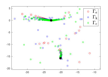
Figure 2: Left panel: Eigenvalue distribution in the complex plane for the three geometries, with $N=1024$ and $\omega=10$, with natural parametrization. Right panel, a detail (zoom at) around the accumulation points, the eigenvalues of $\mathcal{H}_{p,s}$.

   

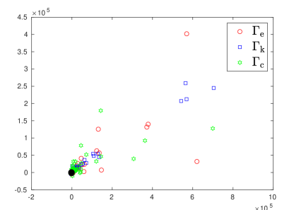
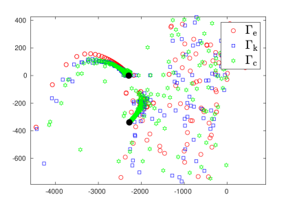
Figure 3: Left panel: Eigenvalue distribution in the complex plane for the three geometries, with $N=1024$ and $\omega=100$. Right panel, a detail (zoom at) around the accumulation points, the eigenvalues of $\mathcal{H}_{p,s}$

$N$	$\Gamma_{\rm e}$		$\Gamma_{\rm k}$		$\Gamma_{\rm c}$
	$\omega=10$	$\omega=100$	$\omega=10$	$\omega=100$	$\omega=10$	$\omega=100$
32	26	65	42	65	39	65
64	24	129	42	129	39	129
128	24	222	41	224	39	233
256	24	234	40	237	39	249
512	24	233	40	238	39	249
1024	24	233	40	238	39	249

Table 3: Number of GMRES iterations required to achieve convergence, using a tolerance level of $10^{-9}$, for the considered geometries. $\Gamma_{\rm e}$ (ellipse), $\Gamma_{\rm k}$ (kite curve) and $\Gamma_{\rm c}$ (the cavity problem) for $\omega=10$ and $\omega=100$. In all these three cases the arc-length parametrization has been used.

$N$	$\Gamma_{\rm e}$		$\Gamma_{\rm k}$		$\Gamma_{\rm c}$
	$\omega=10$	$\omega=100$	$\omega=10$	$\omega=100$	$\omega=10$	$\omega=100$
32	34	65	48	65	50	65
64	34	129	49	129	49	129
128	34	226	50	231	47	235
256	34	234	46	240	44	250
512	34	233	46	238	44	248
1024	34	233	46	235	44	248

Table 4: Number of GMRES iterations required to achieve convergence, using a tolerance level of $10^{-9}$, for the considered geometries. $\Gamma_{\rm e}$ (ellipse), $\Gamma_{\rm k}$ (kite curve) and $\Gamma_{\rm c}$ (the cavity problem) for $\omega=10$ and $\omega=100$. In all these three cases the natural parametrization has been used.

’

7 Conclusions

We analyzed in this paper Nyström discretizations of regularized combined field integral formulations for the solution of Navier scattering problems with smooth boundaries and Dirichlet boundary conditions using the Helmholtz decomposition approach in two dimensions. In order to deliver integral equations of the second kind the regularization strategy we propose relies on compositions of the classical Helmholtz BIOs with approximations of DtN operators. We present and analyze in this paper stable discretizations of these compositions of pseudodifferential operators of opposite orders, both in the simpler case of arclength boundary parametrizations as well as in the more challenging case of general smooth parametrizations. The main idea in the analysis is to isolate via logarithmic kernel splittings the principal parts of the pseudodifferential operators involved and compute explicitly their compositions in the framework of Fourier multipliers. The operator composition of more regular remainders, which are all pseudodifferential operators of negative orders, amounts to simple Nyström matrix multiplication and is amenable to a rather straightforward stability analysis. Extensions to the case of Neumann boundary conditions is currently underway.

Acknowledgments

The first author thanks the support of projects “Adquisición de conocimiento y minería de datos, funciones especiales y métodos numéricos avanzados” from Universidad Pública de Navarra, Spain and “Técnicas innovadoras para la resolución de problemas evolutivos”, ref. PID2022-136441NB-I00 from Ministerio de Ciencia e Innovación, Gobierno de España, Spain. Catalin Turc gratefully acknowledges support from NSF through contract “Optimized Domain Decomposition Methods for Wave Propagation in Complex Media” ref DMS-1908602.

References

• [1] H. Ammari, H. Kang, and H. Lee. Layer potential techniques in spectral analysis, volume 153 of Mathematical Surveys and Monographs. American Mathematical Society, Providence, RI, 2009.
• [2] D. N. Arnold and W.L. Wendland. On the asymptotic convergence of collocation methods. Math. Comp., 41(164):349–381, 1983.
• [3] Y. Boubendir, V. Domínguez, D. Levadoux, and C. Turc. Regularized combined field integral equations for acoustic transmission problems. SIAM Journal on Applied Mathematics, 75(3):929–952, 2015.
• [4] Y. Boubendir, V. Domínguez, David Levadoux, and Catalin Turc. Regularized combined field integral equations for acoustic transmission problems. SIAM J. Appl. Math., 75(3):929–952, 2015.
• [5] Y. Boubendir, C. Turc, and V. Domínguez. High-order Nyström discretizations for the solution of integral equation formulations of two-dimensional Helmholtz transmission problems. IMA J. Numer. Anal., 36(1):463–492, 2016.
• [6] Y. Boubendir, C. Turc, and V. Domínguez. High-order Nyström discretizations for the solution of integral equation formulations of two-dimensional Helmholtz transmission problems. IMA Journal of Numerical Analysis, 36(1):463–492, 03 2015.
• [7] H. Brakhage and P. Werner. Über das Dirichletsche Aussenraumproblem für die Helmholtzsche Schwingungsgleichung. Arch. Math., 16:325–329, 1965.
• [8] O. P. Bruno and T. Yin. Regularized integral equation methods for elastic scattering problems in three dimensions. Journal of Computational Physics, 410:109350, 2020.
• [9] S. Chaillat, M. Darbas, and F. Le Louër. Approximate local Dirichlet-to-Neumann map for three-dimensional time-harmonic elastic waves. Computer Methods in Applied Mechanics and Engineering, 297:62–83, 2015.
• [10] S. Chaillat, M. Darbas, and F. Le Louër. Analytical preconditioners for Neumann elastodynamic boundary element methods. Partial Differ. Equ. Appl., 2(2):Paper No. 22, 26, 2021.
• [11] R. Chapko, R. Kress, and L. Monch. On the numerical solution of a hypersingular integral equation for elastic scattering from a planar crack. IMA journal of numerical analysis, 20(4):601–619, 2000.
• [12] M. Costabel. Boundary integral operators on lipschitz domains: Elementary results. SIAM Journal on Mathematical Analysis, 19(3):613–626, 1988.
• [13] V. Domínguez, S.L. Lu, and F.-J. Sayas. A Nyström flavored Calderón calculus of order three for two dimensional waves, time-harmonic and transient. Comput. Math. Appl., 67(1):217–236, 2014.
• [14] V. Domínguez, S.L. Lu, and F.J. Sayas. A fully discrete Calderón calculus for two dimensional time harmonic waves. Int. J. Numer. Anal. Model., 11(2):332–345, 2014.
• [15] V. Domínguez, S.L. Lu, and F.J. Sayas. A Nyström flavored Calderón calculus of order three for two dimensional waves, time-harmonic and transient. Computers & Mathematics with Applications, 67(1):217–236, 2014.
• [16] V. Domínguez, M.L. Rapún, and F.J. Sayas. Dirac delta methods for Helmholtz transmission problems. Advances in Computational Mathematics, 28(2):119–139, 2008.
• [17] V. Domínguez, T. Sánchez-Vizuet, and F.J. Sayas. A fully discrete Calderón calculus for the two-dimensional elastic wave equation. Comput. Math. Appl., 69(7):620–635, 2015.
• [18] V. Domínguez and C. Turc. High order Nyström methods for transmission problems for Helmholtz equations. In Trends in differential equations and applications, volume 8 of SEMA SIMAI Springer Ser., pages 261–285. Springer, [Cham], 2016.
• [19] V. Domínguez and C. Turc. Boundary integral equation methods for the solution of scattering and transmission 2D elastodynamic problems. IMA J. Appl. Math., 87(4):647–706, 2022.
• [20] V. Dominguez and C. Turc. Robust boundary integral equations for the solution of elastic scattering problems via Helmholtz decompositions, 2022. Submitted.
• [21] H. Dong, J. Lai, and P. Li. A highly accurate boundary integral method for the elastic obstacle scattering problem. Mathematics of Computation, 90:2785–2814, 2021.
• [22] L. M. Faria, C. Pérez-Arancibia, and M. Bonnet. General-purpose kernel regularization of boundary integral equations via density interpolation. Computer Methods in Applied Mechanics and Engineering, 378:113703, 2021.
• [23] G.C. Hsiao and W.L. Wendland. Boundary integral equations. Springer, 2008.
• [24] R. Kress. On the numerical solution of a hypersingular integral equation in scattering theory. J. Comput. Appl. Math., 61(3):345–360, 1995.
• [25] R. Kress. Linear Integral Equations. Applied Mathematical Sciences. Springer New York, 2013.
• [26] V.D. Kupradze. Three-dimensional problems of elasticity and thermoelasticity. Elsevier, 2012.
• [27] R. Kussmaul. Ein numerisches Verfahren zur Lösung des Neumannschen Außenraumproblems für die zweidimensionale Helmholtzsche Schwingungsgleichung. In Methoden und Verfahren der Mathematischen Physik, Band 1 (Bericht über eine Tagung, Oberwolfach, 1969), volume 720/720a* of B. I. Hochschulskripten, pages 15–31. Bibliographisches Inst., Mannheim-Vienna-Zürich, 1969.
• [28] E. Martensen. Über eine Methode zum räumlichen Neumannschen Problem mit einer Anwendung für torusartige Berandungen. Acta Math., 109:75–135, 1963.
• [29] W. McLean. Strongly elliptic systems and boundary integral equations. Cambridge University Press, Cambridge, 2000.
• [30] K. Ruotsalainen and J. Saranen. A dual method to the collocation method. Math. Methods Appl. Sci., 10(4):439–445, 1988.
• [31] J. Saranen and G. Vainikko. Periodic integral and pseudodifferential equations with numerical approximation. Springer Monographs in Mathematics. Springer-Verlag, Berlin, 2002.
• [32] F.-J. Sayas et al. deltaBEM: a MATLAB-based suite for 2-D numerical computing with the boundary element method on smooth geometries and open arcs. In https://team-pancho.github.io/deltaBEM/. Accessed on Date.
• [33] I H. Sloan and W. L. Wendland. Qualocation methods for elliptic boundary integral equations. Numer. Math., 79(3):451–483, 1998.