Heegaard Floer Symplectic homology and Viterbo’s isomorphism theorem in the context of multiple particles

Abstract.

Given a Liouville manifold $M$, we introduce an invariant of $M$ that we call the Heegaard Floer symplectic cohomology $SH^{*}_{\kappa}(M)$ for any $\kappa\geq 1$ that coincides with the symplectic cohomology for $\kappa=1$. Writing $\hat{M}$ for the completion of $M$, the differential counts pseudoholomorphic curves of arbitrary genus in $\mathbb{R}\times S^{1}\times\hat{M}$ that are required to be branched $\kappa$-sheeted covers when projected to the $\mathbb{R}\times S^{1}$-direction; this resembles the cylindrical reformulation of Heegaard Floer homology by Lipshitz. These cohomology groups provide a closed-string analogue of higher-dimensional Heegaard Floer homology introduced by Colin, Honda, and Tian.

When $\hat{M}=T^{*}Q$ with $Q$ an orientable manifold, we introduce a Morse-theoretic analogue of Heegaard Floer symplectic cohomology, which we call the free multiloop complex of $Q$. When $Q$ has vanishing relative second Stiefel-Whitney class, we prove a generalized version of Viterbo’s isomorphism theorem by showing that the cohomology groups $SH^{*}_{\kappa}(T^{*}Q)$ are isomorphic to the cohomology groups of the free multiloop complex of $Q$.

1. Introduction

Since its introduction in Viterbo’s foundational paper [Vit99], symplectic cohomology has emerged as a powerful and useful invariant of Liouville domains. Let $(M,\lambda)$ be a Liouville domain, and $\hat{M}=M\cup_{\partial M}([1,\infty)\times\partial M)$ be its completion. One way to define the symplectic cohomology of $M$ (or of $\hat{M}$) is to count pseudoholomorphic cylinders connecting closed orbits of the usual one-particle motion Hamiltonian system in the completion $\hat{M}$ according to [Sei08, AS10a]. In this paper, we construct an invariant of $M$ where, instead of one-particle motion, we consider the dynamics of multiple identical particles in $\hat{M}$. The closed orbits then can be regarded as loops in the unordered configuration space $\operatorname{UConf}_{\kappa}(\hat{M})$, where $\kappa\geq 1$ is the number of particles under consideration.

Naturally, one would want to count pseudoholomorphic cylinders in the symmetric product $\operatorname{Sym}^{\kappa}(\hat{M})$ connecting orbits as above. The main obstacle is that, in general, the symmetric product of a manifold is not a smooth manifold. One strategy is to study Floer theory of the symplectic orbifold $\operatorname{Sym}^{\kappa}(\hat{M})$ and it has been undertaken in [MS21], based on the approach from [CP14], for $\kappa=2$ to obtain non-dispaceability results for Lagrangian links in $S^{2}\times S^{2}$. Instead, in the present work we study moduli spaces of curves in $\mathbb{R}\times S^{1}\times\hat{M}$ mimicking Lipshitz’s cylindrical reformulation [Lip06] of the Heegaard Floer homology. This provides a closed string analogue of higher-dimensional Heegaard Floer homology (HDHF) introduced by Colin, Honda, and Tian in [CHT20]. We recall that HDHF provides a model for the Lagrangian Floer homology of the symmetric product $\operatorname{Sym}^{\kappa}(M)$.

In this paper, we present two closely related versions of such a sought-after invariant which we refer to as the unsymmetrized version $SH^{*}_{\kappa,\text{unsym}}(M)$ of Heegaard Floer symplectic cohomology (HFSH) and the partially symmetrized version $SH^{*}_{\kappa,\text{psym}}(M)$ of HFSH.

Theorem 1.1 (Theorems 2.41, 2.53 and 2.58).

The Heegaard Floer symplectic cohomology groups $SH^{*}_{\kappa,\text{psym}}(M)$ and $SH^{*}_{\kappa,\text{unsym}}(M)$ are well defined and are invariants of the Liouville domain $M$, independent of all the intrinsic choices of the Floer data required for its setup.

The main obstacle for translating the HDHF setup to the closed string context is that unlike in [CHT20] the tuples of orbits of cumulative time $\kappa$ may contain multiply covered orbits. This may lead to the multiply covered curves in the boundary of moduli spaces of solutions to an appropriate $\bar{\partial}_{J,H}$-equation. The tool we develop here to tackle this issue is a certain perturbation scheme on a branched manifold that we associate with Hurwitz spaces $\mathcal{H}^{\bm{\mu},\bm{\mu}^{\prime}}_{\kappa,\chi}$ serving as moduli spaces of branched $\kappa$-sheeted covers of the cylinder $\mathbb{R}\times S^{1}$. We point out that this setting simplifies numerous problems that arise in the context of higher-genus SFT [EGH00].

Let us now consider the case where $\hat{M}=T^{*}Q$. We recall that Abbondandolo-Schwarz [AS06] and Abouzaid [Abo11] show that for an orientable manifold $Q$ there is an isomorphism between the symplectic cohomology $SH^{*}_{b}(T^{*}Q)$ twisted by a certain background class and the homology of the free loop space of $Q$. Abbondandolo and Schwarz construct a chain map from the Morse complex associated with action functional $\mathcal{A}_{L}$ on the space $\Lambda^{1}(Q)$ of free loops in the class $W^{1,2}$ to the symplectic cochain complex. They prove that this chain map is a quasi-isomorphism, whereas Abouzaid constructs a chain map in the opposite direction and proves that it is the inverse of the former.

In this paper, in an attempt to compute the unsymmetrized version of Heegaard Floer symplectic cohomology, we introduce a Morse-theoretic model which is intended to generalize the Morse complex $CM_{*}(\Lambda^{1}(Q))$. We consider the space $\Lambda^{1}_{\kappa}(Q)$ of free multiloops of class $W^{1,2}$ which can be understood as free loops in $\operatorname{UConf}_{\kappa}(Q)$ of class $W^{1,2}$. The differential of this Morse complex $CM_{*}(\Lambda^{1}_{\kappa}(Q))$ counts not only gradient trajectories but also piecewise gradient trajectories where the multiloops are allowed to undergo switchings at finitely many moments. These switchings are meant to correspond to ramification points on the Heegaard Floer side. This model is parallel to the Morse model for HDHF in [HKTY].

For any orientable manifold $Q$ of dimension $n$ with vanishing second Stiefel-Whitney class $w_{2}(TQ)\in H^{2}(T^{*}Q;\mathbb{Z}/2)$ we then construct a map

$$\mathcal{F}\colon SH_{\kappa,\text{unsym}}^{*}(T^{*}Q)\to CM_{\kappa n-*}(\Lambda^{1}_{\kappa}(Q)),$$

which for $\kappa=1$ coincides with the chain map constructed by Abouzaid. It also extends the map constructed in [HTY ̵a] in the context of HDHF for $Q$ of dimension $2$ to higher dimensions. We then prove the following:

Theorem 1.2 (Theorems 4.20 and 4.11).

For $Q$ an orientable manifold with vanishing second Stiefel-Whitney class $w_{2}(TQ)\leavevmode\nobreak\ \in\leavevmode\nobreak\ H^{2}(T^{*}Q;\mathbb{Z}/2)$ the map $\mathcal{F}$ is a chain map and induces an isomorphism on the homology

$$SH^{*}_{\kappa,\text{unsym}}(T^{*}Q)\cong HM_{\kappa n-*}(\Lambda^{1}_{\kappa}(Q)).$$

In the situation of ordinary symplectic cohomology Abouzaid [Abo11, Abo15] constructs an isomorphism of this kind when $w_{2}(TQ)\neq 0$ between the symplectic cohomology with twisted coefficients and the Morse homology of the free loop space. We hope that $\mathcal{F}$ as above also can be extended to such a more general setting. The first work which highlighted the necessity of twisted coefficients is that of Kragh [Kra18].

There are numerous questions one can ask regarding HFSH and the Morse model above, and here we list just some of them. First, the original symplectic cohomology possesses various algebraic structures and we refer the reader to [Sei08, Rit13, Abo15] for a broad review. Therefore, it is natural to ask:

Question 1.3.

How much of various algebra structures including the BV-algebra structure, Viterbo restriction, TQFT-structure, etc., can be extended from symplectic cohomology to HFSH?

We expect most of the algebraic operations related to symplectic cohomology to have their analogues in the context of HFSH. We further hope that the corresponding structures will come in handy to show the generation criterion for HDHF wrapped Fukaya category $\mathcal{W}_{\kappa}(T^{*}Q)$, extending the result of Abouzaid [Abo10]. More precisely, we pose the following:

Conjecture 1.4.

Given a closed oriented manifold $Q$ with vanishing relative second Stiefel-Whitney class, the HDHF wrapped Fukaya category $\mathcal{W}_{\kappa}(T^{*}Q)$ is split-generated by any $\kappa$-tuple of disjoint cotangent fibers.

Furthermore, based on the work of Ganatra [Gan12] we expect a close relationship between Hochschild homology $HH_{*}(\mathcal{W}_{\kappa}(\hat{M}))$ of the wrapped HDHF Fukaya category and HFSH and we state it as the following:

Question 1.5.

What is the relationship between the Hochschild homology $HH_{*}(\mathcal{W}_{\kappa}(\hat{M}))$ and the Heegaard Floer symplectic cohomology $SH^{*}_{\kappa}(M)$ for $M$ a Liouville domain?

Structure of the paper.

Section 2 is devoted to the setup of Heegaard Floer symplectic cohomology. We first introduce basic definitions and notation in Sections 2.1-2.3 in the context of the partially symmetrized Heegaard Floer symplectic cohomology. In Sections 2.4-2.5 we introduce Hurwitz spaces, which serve as model spaces for the Floer data required to define HFSH. Our treatment is based on the long lineage of work devoted to the study of Hurwitz schemes, for instance, [ACV03, Deo14, HM98, HM82, Ion02, Prü17]. We adapt this circle of ideas to our particular problem in the SFT setting. Furthermore, we introduce a branched manifold structure on the Hurwitz spaces in the sense of [McD06] in Section 2.6 and assign consistent Floer data to Hurwitz spaces.

In Sections 2.9-2.11 we show that the above data indeed provide a chain complex $SC_{\kappa,\text{unsym}}(\hat{M};H,J)$, where $(H,J)$ denotes some Floer data adapted to a quadratic at infinity Hamiltonian function $H_{0}$ and a time-dependent almost complex structure $J_{t}$. Following the original approach in [Sei08] we give an alternative definition of the partially symmetrized HFSH via tuples of linear Hamiltonian functions in Section 2.12. We also show that this definition via the direct limit over all tuples of linear Hamiltonians coincides with the definition given by means of a quadratic at infinity $H_{0}$ as above. The approach in terms of linear Hamiltonians is known to provide a simple way of showing the invariance of symplectic cohomology and we adopt it to show that the partially symmetrized HFSH also gives an invariant of a Liouville domain $M$.

In Section 3 we introduce the free multiloop complex associated with an oriented manifold $Q$. This section is mostly devoted to showing that multiloops with a differential given by counting piecewise pseudo-gradient trajectories form a chain complex. The methods we use rely greatly on the approach of Abbondandolo-Schwarz in [AS10] and Abbondandolo-Majer in [AM06].

In Section 4 we prove Theorem 1.2. The chain map is constructed by means of moduli spaces of pseudoholomorphic curves associated with branched $\kappa$-sheeted covers of the half-cylinder $\mathbb{R}_{\geq 0}\times S^{1}$ extending the ideas in [Abo11, Abo15] to the Heegaard Floer context.

Acknowledgements. RK and TY thank Ko Honda for his guidance and emotional support. RK also thanks Sheel Ganatra, Robert Lipshitz, Cheuk Yu Mak, Ivan Smith, Gleb Terentiuk and Bogdan Zavyalov for stimulating discussions. RK would also like to thank the organizers of the Symplectic Paradise summer school for creating an inspiring atmosphere that influenced the work on this project. TY thanks Yin Tian for helpful discussions. TY is supported by China Postdoctoral Science Foundation 2023T160002 and 2023M740106.

2. The Floer complex

2.1. The Liouville manifold

Let $(M,\lambda)$ be a $2n$-dimensional Liouville domain, i.e., $M$ is a compact exact symplectic manifold with boundary, $\lambda$ is a primitive of a symplectic form, and the Liouville vector field $V$ (satisfying $L_{V}d\lambda=d\lambda$) points outwards along the boundary $\partial M$.

The Liouville form $\lambda$ restricts to a contact form $\alpha\coloneqq\lambda|_{\partial M}$ on $\partial M$. We then complete $M$ to $\hat{M}$ by attaching the symplectization end $([1,\infty)_{r}\times\partial M,r\alpha)$ along $\partial M$. Denote the Reeb vector field of $(\partial M,\alpha)$ by $R$. We require that

• all Reeb orbits of $\alpha$ are non-degenerate.

To define an integral grading for the Floer complex, we further require that

• $2c_{1}(M)\in H^{2}(M,\mathbb{Z})$ vanishes.

2.2. Tuples of Hamiltonian orbits

Here, we introduce the cochain complex for the partially symmetrized version of Heegaard Floer symplectic cohomology. The cochains to be introduced correspond to tuples of Hamiltonian orbits of some function of cumulative time $\kappa$. Describing them in this context requires working separately with each partition of $\kappa$. That is why we would have to reserve significantly more Hamiltonians than $\kappa$, which is enough for the unsymmetrized version; see Section 2.13.

Let $\bm{\mu}=(\mu_{1},\ldots,\mu_{l(\bm{\mu})})$ satisfying $\mu_{1}\geq\mu_{2}\geq\ldots\geq\mu_{l(\bm{\mu})}$ be a partition of $\kappa$, where $l(\bm{\mu})$ denotes the length of $\bm{\mu}$, i.e., the number of elements in the partition. Following standard notation, we set $\bm{\mu}!\coloneqq\mu_{1}\cdot\ldots\cdot\mu_{l(\bm{\mu})}$. We put

(2.1) $$m_{i}(\bm{\mu})=\#\{j\colon\mu_{j}=i\},$$

(2.2) $$R_{\bm{\mu}}=\prod_{i}m_{i}(\bm{\mu})!,$$

(2.3) $$N_{\bm{\mu}}=\bm{\mu}!\cdot R_{\bm{\mu}}.$$

For the $i$-th element $\mu_{i}$ of the partition $\bm{\mu}$ we assign an additional ordering given by $ord_{i}(\bm{\mu})=i-\sum_{\mu_{i}<k\leq\mu_{1}}m_{k}(\bm{\mu})$. This ordering is meant to record the encountering of each particular value in the partition $\bm{\mu}$, e.g., for $\bm{\mu}=(2,2,1,1,1)$ we have $ord_{4}(\bm{\mu})=2$ and therefore $\mu_{4}$ is the second term in this partition of value $\mu_{4}=1$.

Let $H_{0}\colon S^{1}_{t}\times\hat{M}\to\mathbb{R}$ be a time independent Hamiltonian function on $\hat{M}$, which is quadratic away from some compact subset of $\hat{M}$, i.e., $H_{0}=r^{2}/2$ on $[R,\infty)_{r}\times\partial M$ for some $R\geq 1$. We denote the class of such functions by $\mathcal{H}(\hat{M})\subset C^{\infty}(S^{1}\times\hat{M})$. We choose $F_{0}\colon S^{1}\times\hat{M}\to\mathbb{R}$ to be a smooth nonnegative function satisfying:

1. the functions $F_{0}$ and $\lambda(X_{F_{0}})$ are uniformly bounded in absolute value;

2. all time-$1$ periodic orbits of $X_{H_{0}^{\text{tot}}}$, the Hamiltonian vector field of the function $H_{0}^{\text{tot}}=H_{0}+F_{0}$, are non-degenerate.

The choice of such $F_{0}$ for a given $H_{0}\in\mathcal{H}(M)$ exists by [Abo10, Lemma 5.1]. As we are interested in tuples of Hamiltonian orbits of $H^{\text{tot}}_{0}$ of cumulative time $\kappa$ we now introduce further perturbations to ensure that such tuples are non-degenerate. That is, we choose a collection of functions $F_{m,j}$ for $1\leq m\leq\kappa$, $1\leq j\leq\lfloor\frac{\kappa}{m}\rfloor$ satisfying

1. $F_{m,j}\colon\mathbb{R}/m\mathbb{Z}\times\hat{M}\longrightarrow\mathbb{R}$ is non-negative such that $|F_{m,j}-F_{0}|$ is absolutely bounded by a small constant and vanishes away from the locus of time-$m$ orbits of $H^{\text{tot}}_{0}$;

2. all time-$m$ orbits of $H^{\text{tot}}_{m,j}=H_{0}+F_{m,j}$ are non-degenerate and each such orbit lies in a small neighborhood of the corresponding time-$m$ orbits of $H^{\text{tot}}_{0}$;

3. Hamiltonian time-$m$ orbits for different $H^{\text{tot}}_{m,j}$’s are disjoint and embedded;

We further denote the collections of Hamiltonians $\bm{H}^{\text{tot}}=\{H^{\text{tot}}_{m,j}\}$ satisfying all of the above properties by ${\mathcal{\bm{H}}}_{S^{1}}^{\kappa}(\hat{M})$.

Let us note that, due to rotational symmetry, a non-multiply covered time-$m$ orbit of $H_{0}^{\text{tot}}$ it corresponds to $m$ orbits of $H_{0}^{\text{tot}}$ with the same image. Therefore, these $m$ orbits produce $m$ distinct orbits of $H^{\text{tot}}_{m,j}$ for any $j$, $1\leq j\leq\lfloor\frac{\kappa}{m}\rfloor$. See Figure 1 for an illustration of this phenomenon with $m=2$.

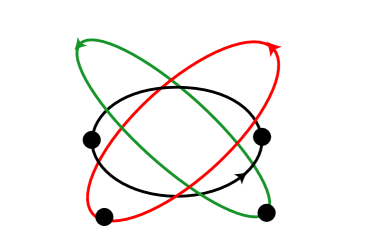
Figure 1. The black curve denotes a time-$2$ orbit of $H_{0}^{\text{tot}}$. The green and red curves denote the two nearby orbits of $H^{\text{tot}}_{2,1}$. The dots correspond to the starting points of these orbits.

More generally, assume we are given a tuple of Hamiltonian orbits of $H^{\text{tot}}_{0}$ of cumulative time $\kappa$ with no multiply covered orbits among them, and let the periods of these orbits form a partition $\bm{\mu}$ of $\kappa$. There are $R_{\bm{\mu}}$ ways to order these orbits preserving the time-ordering. Given such an order on the orbits $x_{1},\ldots,x_{\ell(\bm{\mu})}$, there are $\bm{\mu}!$ distinct tuples of orbits of the form $x_{1}^{\prime},\ldots,x_{\ell(\bm{\mu})}^{\prime}$, where each $x_{i}^{\prime}$ is a Hamiltonian orbit of $H^{\text{tot}}_{\mu_{i},ord_{i}(\bm{\mu})}$. All these $\mu!$ tuples are in the small neighborhood of the initial tuple $x_{1},\ldots,x_{\ell(\bm{\mu})}$. Hence, in total near the initial tuple, there are $N_{\bm{\mu}}$ new “desymmetrized” tuples with disjoint images, since there are $R_{\bm{\mu}}$ orderings and a total of $\bm{\mu}!$ rotations.

We set $\mathcal{P}_{\text{psym}}$ to be

(2.6) $$\mathcal{P}_{\text{psym}}\coloneqq\left\{\bm{x}=(x_{1},\ldots,x_{l(\bm{\mu})})\left|\begin{array}[]{ll}\text{$x_{i}\colon[0,\mu_{i}]\to\hat{M}$ is the integral flow of $\phi^{t}_{H^{\text{tot}}_{\mu_{i},ord_{i}(\bm{\mu})}}$,}\\ \text{$x_{i}(0)=x_{i}(\mu_{i})$, $\bm{\mu}$ is a partition of $\kappa$.}\end{array}\right.\right\}$$

Figure 2. A sample tuple of Hamiltonian orbits in $\mathcal{P}_{\text{psym}}$ for $\kappa=5$.

To an orbit $x_{\mu_{i}}$ we associate a differential operator

(2.7) $$D_{x_{\mu_{i}}}\colon W^{1,2}(\mathbb{C},\mathbb{C}^{n})\to L^{2}(\mathbb{C},\mathbb{C}^{n}),$$

following [Abo10, Section C.6]. Using this operator, one defines the orientation line of $x_{\mu_{i}}$

(2.8) $$o_{x_{\mu_{i}}}=|\operatorname{det}(D_{x_{\mu_{i}}})|,$$

i.e., $o_{x_{\mu_{i}}}$ is a rank-$1$ free abelian group with two generators representing two possible orientations of $\operatorname{det}(D_{x_{\mu_{i}}})$ and the relation that their sum is zero; see Section 2.14 for the notations that we use here.

Definition 2.1.

The orientation line $o_{\bm{x}}$ of $\bm{x}\in\mathcal{P}_{\text{psym}}$ is given as follows:

(2.9) $$o_{\bm{x}}=o_{x_{\mu_{1}}}\otimes\ldots\otimes o_{x_{\mu_{\ell(\bm{\mu})}}}.$$

Regarding $o_{\bm{x}}$ as a $\mathbb{Z}$-module we set

(2.10) $$o_{\bm{x}}^{\mathbb{Q}}=\mathbb{Q}\otimes_{\mathbb{Z}}o_{\bm{x}}$$

We then set

(2.11) $$V_{\kappa,\text{psym}}=\bigoplus_{\bm{x}\in\mathcal{P}_{\text{psym}}}o_{\bm{x}}^{\mathbb{Q}}.$$

Each $\bm{x}\in\mathcal{P}_{\text{psym}}$ comes with a grading that we discuss in Section 2.3. Hence the above is a graded vector space with

(2.12) $$V^{i}_{\kappa,\text{psym}}=\bigoplus_{|\bm{x}|=i}o_{\bm{x}}^{\mathbb{Q}}.$$

Consider a formal variable $\hbar$ with grading $|\hbar|=2-n$. We then set $SC^{*}_{\kappa,\text{psym}}(\hat{M})$ to be a graded vector subspace in $V_{\kappa,\text{psym}}[[\hbar]]$

(2.13) $$SC_{\kappa,\text{psym}}^{m}(\hat{M})\coloneqq\sum_{i+(2-n)j=m}V^{i}_{\kappa,\text{psym}}\hbar^{j}=\sum_{i+(2-n)j=m}V^{i}_{\kappa,\text{psym}}\bigl{[}(n-2)j\bigr{]},$$

where in the last term we used the shift convention from Section 2.14 and the summation sign means direct product. We notice that this space is a graded $\mathbb{Q}[h]$-module (but it is not a $\mathbb{Q}[[\hbar]]$-module). In particular, multiplication by $\hbar$ induces a $(2-n)$-degree shift on $SC^{*}_{\kappa,\text{psym}}(\hat{M})$.

For each tuple of Hamiltonian orbits $\bm{x}=(x_{1},\ldots,x_{\ell(\bm{\mu})})\in\mathcal{P}_{\text{psym}}$, we define the action of $\bm{x}$ by

(2.14) $$\mathcal{A}(\bm{x})=\sum^{\ell(\bm{\mu})}_{i=1}\mathcal{A}(x_{i}).$$

where the action of the orbit $x_{i}$ is given by the expression

(2.15) $$\mathcal{A}(x_{i})=\int^{\mu_{i}}_{0}x_{i}^{*}\lambda-\int^{\mu_{i}}_{0}H^{\text{tot}}_{\mu_{i},ord_{i}{\bm{\mu}}}(t,x_{i}(t))dt,$$

We will further denote by $\bm{\mu}(\bm{x})\vdash\kappa$ the partition associated with $\bm{x}$. A tuple of Hamiltonian orbits $\bm{x}$ can be also viewed as a loop in $\mathrm{Conf}_{\kappa}(\hat{M})$ by considering a collection of $\kappa$ paths, where each path takes the form $\gamma\colon[0,1]\rightarrow\hat{M}$ with

$$\gamma(t)\equiv x_{i}(k+t),\,t\in[0,1]$$

for some $x_{i}\in\bm{x}$ and $k\in\mathbb{Z}$ such that $0\leq k<\mu_{i}$.

Remark 2.2.

The main difference between $\mathcal{P}_{\text{unsym}}$ and $\mathcal{P}_{\text{psym}}$ which we introduce in Section 2.13, is that an unperturbed loop in $\mathrm{Conf}_{\kappa}(\hat{M})$ (given by $\kappa$ time-$1$ flows of $H_{0}$) provides $\kappa!$ elements of $\mathcal{P}_{\text{unsym}}$ and only $N_{\bm{\mu}}$ (see (2.2) and (2.3)) elements of $\mathcal{P}_{\text{psym}}$, where $\bm{\mu}!$ stands for a number of ways to choose a starting point on each of the orbits and $R_{\bm{\mu}}$ is responsible for ordering the orbits.

In the toy example with a tuple consisting of Hamiltonian orbits of $H_{0}$ of respective times $\bm{\mu}=(2,1,1)$ we have $\bm{\mu}!=2$, as there are two ways to pick the starting point on the time-$2$ orbit, and $N_{\bm{\mu}}=2$ as there are two ways to give an order on the $2$ time-$1$ orbits. Therefore, in this example $\#\mathcal{P}_{\text{psym}}=4$ and $\#\mathcal{P}_{\text{unsym}}=24$.

2.3. Almost complex structures and gradings

Denote the contact hyperplane field $\operatorname{Ker}\lambda|_{\partial M}\subset T(\partial M)$ by $\xi$. Then we can write

(2.16) $$T([1,\infty)\times\partial M)=\mathbb{R}^{2}\oplus\xi,$$

where $\mathbb{R}^{2}$ is spanned by $\partial_{r}$ and the Reeb vector field $R$.

Let $\mathcal{J}(\hat{M})$ be the set of almost complex structures on $\hat{M}$ tamed by $d\lambda$ which are of rescaled contact type on the symplectization end:

(2.17) $$-\frac{1}{r}\lambda\circ J=dr,$$

that is,

(2.20) $$\left\{\begin{array}[]{ll}J\colon\xi\to\xi,\\ J(R)=\partial_{r},\end{array}\right.$$

on $[1,\infty)\times\partial M$ for $J\in\mathcal{J}(\hat{M})$. From now on we fix a generic family of almost complex structures of rescaled contact type

(2.21) $$J_{t}\colon[0,1]\to\mathcal{J}(\hat{M}).$$

Given any almost complex structure in $\mathcal{J}(\hat{M})$, we can define a grading on $SC_{\kappa}(\hat{M})$. Since $2c_{1}(M)=0$, the bicanonical bundle $(\Lambda_{\mathbb{C}}^{2}T^{*}\hat{M})^{\otimes 2}$ is trivial. One can then define the usual Conley-Zehnder indices of Hamiltonian orbits.

For a tuple of Hamiltonian orbits $\bm{x}\in\mathcal{P}_{\text{psym}}$ we set its grading as well as the grading of the associated orientation line $o_{\bm{x}}$ to be

(2.22) $$|\bm{x}|=\operatorname{deg}(o_{\bm{x}})=\kappa n-CZ(x_{1})-\ldots-CZ(x_{\ell(\bm{\mu}(\bm{x}))}).$$

Remark 2.3.

Note that for $\kappa=1$ the grading above agrees with the convention in [Abo10].

2.4. Moduli space of marked cylinders

Definition 2.4.

A stable cylinder is a tuple $\bm{C}=(C,j,B,D)$, where

• $(C,j)$ is Riemann surface consisting of the main component which is a cylinder $C_{0}=\mathbb{R}_{s}\times S^{1}_{t}$ with $j|_{C_{0}}$ a standard complex structure and a collection of projective planes (i.e., $\mathbb{C}\mathbb{P}^{1}$’s up to biholomorphism) with $j$ restricting to the standard complex structure;

• $B$ is the finite ordered tuple comprised of marked points $q_{1},\ldots,q_{|B|}$ on $C$;

• $D$ is the set consisting of unordered nonintersecting pairs of points $\{d,d^{\prime}\}\subset C$ which are disjoint from $B$ and belong to different components, where any such pair represents a node.

• each component is stable;

• the nodal Riemann surface $\bm{C}^{D}\coloneqq C/\sim_{D}$, where $d\sim_{D}d^{\prime}$ if $\{d,d^{\prime}\}\in D$, is connected and the genus of $\bm{C}^{D}$ equals $0$.

Essentially, one may regard the main component $\mathbb{R}_{s}\times S^{1}_{t}$ as a sphere $\mathbb{P}^{1}$ punctured at $2$ marked points $q_{+\infty}=\infty\in\mathbb{P}^{1}$ and $q_{-\infty}=0\in\mathbb{P}^{1}$. Compactifying the main component yields a genus $0$ curve with two marked points $q_{-\infty}$ and $q_{+\infty}$. From this perspective, assuming that $|B|=k$, stable cylinders up to automorphism (by this we mean biholomorphisms that preserve $B$ as an ordered set, and $D$ as a set) may be regarded as a part of Deligne-Mumford compactification $\overline{\mathcal{M}}_{0,k+2}$ of the moduli space of genus zero curves with $k+2$ marked points $(q_{+\infty},q_{-\infty},q_{1},\ldots,q_{k})$. Namely, classes of stable cylinders up to isomorphism are in bijection with automorphism classes of genus zero nodal curves with $q_{+\infty}$ and $q_{-\infty}$ staying in the same rational component.

For the main component of a given stable cylinder $\bm{C}$ as above to be stable, it has to contain at least one special point (a marked point or a node). A cylinder $\mathbb{R}\times S^{1}$ with no special points would be further called a trivial cylinder.

We also note that one may identify $S^{1}\times\{\pm\infty\}$ with the corresponding space of tangent directions

(2.23) $$S_{q_{\pm\infty}}\mathbb{P}^{1}=T_{q_{\pm\infty}}\mathbb{P}^{1}/\mathbb{R}.$$

We denote the set of all stable cylinders with $b$ marked points by $\widetilde{\mathcal{C}}_{b}$. Denote by $\widetilde{\mathcal{C}}_{b}$ the space of stable cylinders (i.e., cylindrical buildings of height $1$ without nodes) with $b$ marked points and by $\mathcal{C}_{b}$ its quotient by the $\mathbb{R}$-action on the cylindrical component and by all biholomorphisms on the rational components.

Definition 2.5.

A cylindrical building of height $n$ is a Riemann surface

$$\bm{C}=(\overrightarrow{C}=(C_{1},\ldots,C_{n}),j,B,D=D_{r}\cup D_{s}),$$

where each $C_{i}$ is a stable cylinder and $B$ is an ordered set of marked points obtained as a union of marked points of each $C_{i}$. The set of regular nodes $D_{r}$ is an unordered collection of nodes of all the $C_{i}$ and the set of special nodes $D_{s}$ is a set of all the pairs $\{0_{i},\infty_{i+1}\}$, where $0_{i}$ is a point $0$ of the main component of $C_{i}$ and $\infty_{i+1}$ is a point $\infty$ of the main component of $C_{i+1}$.

Notice that by smoothing all the nodes (together with special ones) of the height $n$ cylindrical building one obtains a genus $0$ connected nodal Riemann surface.

We denote the set of all cylindrical buildings of height $n$ with $b$ marked points by $\widetilde{\mathcal{C}}_{b,n}$. In the special case of $n=1$ we have $\widetilde{\mathcal{C}}_{b,1}=\widetilde{\mathcal{C}}_{b}$.

Definition 2.6.

We say that a cylindrical building $\bm{C}$ of height $n$ is smooth if the set $D_{r}$ is empty; equivalently each $C_{i}$ consists only of the main component.

We denote the set of smooth cylindrical buildings of height $n$ by $\widetilde{\mathcal{C}}^{\text{sm}}_{b,n}$. On $\widetilde{\mathcal{C}}^{\text{sm}}_{b,n}$ there is a natural $\mathbb{R}^{n}$-action given by vertical parallel transports on the main components of the $C_{i}$’s. Let us denote the quotient by

(2.24) $$\widehat{\mathcal{C}}_{b,n}=\widetilde{\mathcal{C}}^{\text{sm}}_{b,n}/\mathbb{R}^{n}.$$

Similarly, we denote by $\mathcal{C}_{b,n}$ the quotient of $\widetilde{\mathcal{C}}_{b,n}$ by the above-mentioned $\mathbb{R}^{n}$-action on the main components and further action by biholomorphisms on the compact components.

For any cylindrical building $\bm{C}$ of height $n$ we denote by $\text{Aut}_{v}(\bm{C})$ the group of vertical automorphisms that acts by vertical translations on the main components and is the $\mathbb{R}^{n}$ by which we have been taking quotients above, e.g. in (2.24).

Remark 2.7.

We stress that we are not going to quotient out the $S^{1}$-action on the main components in our considerations.

By taking the disjoint union of all $\mathcal{C}_{b,n}$ one obtains a moduli space

(2.25) $$\overline{\mathcal{C}}_{b}=\bigsqcup\limits_{n\in\mathbb{Z}_{>0}}\mathcal{C}_{b,n}.$$

It has a subspace $\widehat{\mathcal{C}}_{b}\subset\overline{\mathcal{C}}_{b}$ serving as a moduli space of smooth cylindrical buildings

(2.26) $$\widehat{\mathcal{C}}_{b}=\bigsqcup_{n\in\mathbb{Z}_{>0}}\,\widehat{\mathcal{C}}_{b,n}.$$

Remark 2.8.

The space $\widehat{\mathcal{C}}_{b}$ is the portion of the full compactification $\overline{\mathcal{C}}_{b}$ of our main interest, as for the actual moduli space of pseuholomorphic curves all other forms of degeneration do not appear generically; see Section 2.10. We use hat-notation to describe the portion of a “presumable” compactification consisting of curves with multiple smooth (i.e., without nodes) levels.

Remark 2.9.

Notice that for a given convergent sequence $\bm{C}_{k}$ of smooth cylindrical buildings such that no two marked points “collide” it holds that $\lim_{k\rightarrow\infty}\bm{C}_{k}\in\widehat{\mathcal{C}}_{b}$.

Remark 2.10.

The set of cylindrical buildings up to obvious automorphism (by this we mean automorphisms that restrict to automorphisms of each $C_{i}$) forms the full Deligne-Mumford compactification $\overline{\mathcal{M}}_{0,k+2}$. The height of a building is just the distance between the leaves corresponding to $q_{+\infty}$ and $q_{-\infty}$ in the tree associated with the building regarded as a nodal rational curve.

We set the topology on these spaces following [BEHWZ03]. One can show that

Lemma 2.11.

The space $\overline{\mathcal{C}}_{b}$ is a compact metric space and serves as the compactification of the space $\mathcal{C}_{b}$, i.e., it coincides with the closure of $\mathcal{C}_{b}$ viewed as a subspace of $\overline{\mathcal{C}}_{b}$. In particular, every sequence of smooth cylinders with $b$ marked points has a subsequence that converges to a cylindrical building.

Sketch of the proof.

For simplicity, assume we are given a sequence of smooth cylinders $\bm{C}_{n}\in\mathcal{C}_{b}$. Following [HT07, Section 2] one can pick a subsequence $\bm{C}_{n_{k}}$ with marked points denoted by $q_{1}^{k},\ldots,q_{b}^{k}$ and a partition $\bm{\mu}\vdash b$, such that

• there is a constant $D$ satisfying $\forall j,j^{\prime}\in\mu_{i}\colon\text{dist}(q^{k}_{j},q_{j^{\prime}}^{k})<D$ for any term $\mu_{i}$ of $\bm{\mu}$;

• if $j$ and $j^{\prime}$ do not belong to the same element of $\bm{\mu}$, then $\text{dist}(q_{j}^{k},q_{j^{\prime}}^{k})>k$.

In other words, one may divide branched points into “clusters” such that $t$-coordinate difference between points of different clusters goes to $\infty$. Moreover, the elements of $\bm{\mu}$ can be ordered by their height (i.e., the $t$-coordinates of elements of one cluster are bigger than the $t$-coordinates of the points in another cluster). If no branched points “collide” then the limit of such sequence would be a smooth height $\ell(\bm{\mu})$ cylindrical building. Otherwise, there would appear bubbles and the limit would be a stable height $\ell(\bm{\mu})$ cylindrical building. ∎

For further usage, we note that boundary $\partial\overline{\mathcal{C}}_{b}$ can be covered by images of the natural maps

(2.27) $$\bigsqcup_{b_{1}+b_{2}=b}\overline{\mathcal{C}}_{b_{1}}\times\overline{\mathcal{M}}_{b_{2}}\to\partial\overline{\mathcal{C}}_{b},$$

(2.28) $$\bigsqcup_{b_{1}+b_{2}=b}\overline{\mathcal{C}}_{b_{1}}\times\overline{\mathcal{C}}_{b_{2}}\to\partial\overline{\mathcal{C}}_{b},$$

where the space $\overline{\mathcal{M}}_{b_{2}}$ in (2.27) refers to bubbling on the body of a cylinder and (2.28) describes the appearance of a new level in the building.

Remark 2.12.

Despite forcing out levels that could be trivial cylinders for elements of $\overline{\mathcal{C}}_{b}$ later on we would consider cylindrical buildings with a finite number of trivial cylinders inserted between some of the levels. Clearly, a sequence of cylindrical buildings that converges to an element of $\overline{\mathcal{C}}_{b}$ also converges to the one obtained this way.

To shed more light on the relation between moduli space of cylindrical buildings $\overline{\mathcal{C}}_{b}$ and $\overline{\mathcal{M}}_{0,b+2}$ (see Remark 2.10) we note that there is an $U(1)$-principal bundle

(2.29) $$U(1)\to\widehat{\mathcal{C}}_{b,1}\to\mathcal{M}_{0,b+2},$$

where the $U(1)$ acts by counterclockwise rotations on a given cylinder. Denote by $\mathcal{M}_{0,(b_{1}+2,b_{2}+2)}$ the subset of $\partial\overline{\mathcal{M}}_{0,b+2}$ consisting of nodal curves with $2$ components $S_{1}$, $S_{2}$, such that $q_{+\infty}\in S_{1},q_{-\infty}\in S_{2}$ and $b_{1}+b_{2}=b$. Then there is a principal bundle

(2.30) $$U(1)^{2}\to\widehat{\mathcal{C}}_{b,2}\to\mathcal{M}_{0,(b_{1}+2,b_{2}+2)},$$

and more generically there is $U(1)^{n}$-principal bundle

(2.31) $$U(1)^{n}\to\widehat{\mathcal{C}}_{b,n}\to\mathcal{M}_{0,(b_{1}+2,b_{2}+2,\ldots,b_{n}+2)}$$

where the last space is defined similarly.

We note that $\mathcal{M}_{0,(b_{1}+2,b_{2}+2)}$ is the image of the natural map

(2.32) $$\mathcal{M}_{0,b_{1}+2}\times\mathcal{M}_{0,b_{2}+2}\to\overline{\mathcal{M}}_{0,b+2}$$

given by gluing two curves $(C_{1};q_{+\infty},q_{1},\ldots,q_{b_{1}},q_{-\infty})$ and $(C_{2};q^{\prime}_{+\infty},q^{\prime}_{1},\ldots,q^{\prime}_{b_{2}},q^{\prime}_{-\infty})$ at the node $\{q_{-\infty},q^{\prime}_{+\infty}\}$.

We denote by $L_{q_{i}}$ the line bundle over $\overline{\mathcal{M}}_{0,b+2}$ with fiber $T_{q_{i}}^{*}C$ over

$$(C;q_{+\infty},q_{1},\ldots,q_{b_{1}},q_{-\infty})\in\overline{\mathcal{M}}_{0,b+2}.$$

We now recall facts from deformation theory following [Ion02]; we refer the reader to the related descriptions of a neighborhood of a boundary stratum given in [HK14], [IP04], [Sie97]. Namely, the local coordinates in the normal direction near $\mathcal{M}_{0,(b_{1}+2,b_{2}+2)}$ are given by

(2.33) $$\zeta\in L^{*}_{q_{-\infty}}\otimes L^{*}_{q^{\prime}_{+\infty}},$$

which is a line bundle over $\mathcal{M}_{0,(b_{1}+2,b_{2}+2)}$ with fiber $T_{q_{-\infty}}C_{1}\otimes T_{q^{\prime}_{+\infty}}$. It turns out that the line bundle given in (2.33) is essentially the normal complex line bundle to $\mathcal{M}_{0,(b_{1}+2,b_{2}+2)}\subset\overline{\mathcal{M}}_{0,b+2}$. In local coordinates $(w_{1},w_{2})$ on $C_{1}$ and $C_{2}$ near the node

$$w_{1}w_{2}=0$$

the curve associated with $\zeta$ is locally a solution of

(2.34) $$w_{1}w_{2}=\zeta.$$

Analogously, we may define a complex line bundle

(2.35) $$\hat{L}^{*}_{q_{-\infty}}\otimes\hat{L}^{*}_{q^{\prime}_{+\infty}}$$

on $\widehat{\mathcal{C}}_{b,2}$ with fiber $T_{q_{-\infty}}C_{1}\otimes T_{q^{\prime}_{+\infty}}C_{2}$ at a point $((C_{1};q_{+\infty},\ldots,q_{-\infty}),(C_{2};q^{\prime}_{+\infty},\ldots,q^{\prime}_{-\infty}))$. More explicitly, over $\widetilde{\mathcal{C}}_{b,2}$ both bundles with fibers $T_{q_{-\infty}}C_{1}$ and $T_{q^{\prime}_{+\infty}}C_{2}$ are trivializable (by the means of global coordinates on cylinders) and $\mathbb{R}^{2}$-equivariant. Thus, these vector bundles induce quotient vector bundles on $\widehat{\mathcal{C}}_{b,2}$ which we denote by $\hat{L}^{*}_{q_{-\infty}}$ and $\hat{L}^{*}_{q^{\prime}_{+\infty}}$. We additionally note that projectivizations of real vector bundles $\hat{L}^{*}_{q_{-\infty}}$ and $\hat{L}^{*}_{q^{\prime}_{+\infty}}$ are trivial. Hence, for (2.35) viewed as a real $2$-dimensional bundle there is a global choice of angle coordinate $\varphi$.

We now describe a normal neighborhood of $\widehat{\mathcal{C}}_{b,2}\subset\widehat{\mathcal{C}}_{b}$ similar to (2.33). First, we pick a global section of $\widetilde{\mathcal{C}}_{b,2}\to\widehat{\mathcal{C}}_{b,2}$ as follows. Given a representative

$$((C_{1};q_{+\infty},\ldots,q_{-\infty}),(C_{2};q^{\prime}_{+\infty},\ldots,q^{\prime}_{-\infty}))$$

of a point in $\widehat{\mathcal{C}}_{b,2}$ we assign to it another representative of the same point $(\widetilde{C}_{1},\widetilde{C}_{2})$ obtained by translating $C_{1}$ vertically by a negative of the minimum of the $s$-coordinates of its marked points and translating $C_{2}$ by a negative of the maximum of the $s$-coordinates of its marked points (to make such section smooth one should pick smooth approximations of $min$ and $max$ differing by not more than a constant). The point $(\widetilde{C}_{1},\widetilde{C}_{2})$ will then always have all marked points of $\widetilde{C}_{1}$ above $s=0$ and all marked points of $\widetilde{C}_{2}$ below $s=0$.

Now pick an $R\in(0,+\infty]$ and glue $(\widetilde{C}_{1},\widetilde{C}_{2})$ via the standard procedure. Namely, set

$$\widetilde{C}_{1}^{R}=\widetilde{C}_{1}\setminus(-\infty,-R]\times S^{1},$$

$$\widetilde{C}_{2}^{R}=\widetilde{C}_{2}\setminus[R,+\infty)\times S^{1},$$

$$\widetilde{C}^{R}=\widetilde{C}_{1}^{R}\sqcup\widetilde{C}_{2}^{R}/\sim,$$

where the identification $\sim$ is given by solving

(2.36) $$e^{s_{1}+2\pi\sqrt{-1}t_{1}}\cdot e^{-s_{2}-2\pi\sqrt{-1}t_{2}}=e^{-R}$$

for $-R\leq s_{1}\leq 0$ and for $R=+\infty$ we have $\widetilde{C}^{R}=\widetilde{C}_{1}^{R}\sqcup\widetilde{C}_{2}^{R}$.

Hence, we just constructed a diffeomorphism of a neighborhood of $\widehat{C}_{b,2}\subset\widehat{C}_{b}$ and

(2.37) $$\widehat{C}_{b,2}\times[0,+\infty].$$

Let us notice that given a parameter $R$ as above we can assign a section

(2.38) $$\tilde{\zeta}\in\hat{L}^{*}_{q_{-\infty}}\otimes\hat{L}^{*}_{q^{\prime}_{+\infty}}$$

with $\varphi(\tilde{\zeta})=0$ (recall $\varphi$ is the angular coordinate) and, moreover, $\tilde{\zeta}=e^{R}$ in the local trivialization associated with $(\widetilde{C}_{1},\widetilde{C}_{2})$ as in (2.36). Hence in local coordinates on cylinders, the equation (2.36) is given via

(2.39) $$w_{1}w_{2}=\tilde{\zeta},$$

which is the analogue of (2.34). We point out that unlike in the case of moduli space of curves $\mathcal{M}_{0,b+2}$ the only sections of $\hat{L}^{*}_{q_{-\infty}}\otimes\hat{L}^{*}_{q^{\prime}_{+\infty}}$ that give a family of curves close to breaking are those with $\varphi=0$.

More generally, there is a similar description of a neighborhood of $\widehat{C}_{b,n}$ diffeomorphic to

(2.40) $$\widehat{C}_{b,n}\times[0,+\infty]^{n-1}.$$

Given any curve $C$ and a point $q\in C$ we introduce the notation

(2.41) $$\mathcal{S}^{1}_{q}\bm{C}=(T_{q}C\setminus\{0\})/\mathbb{R}_{\geq 0}.$$

For a nodal curve $\bm{C}$ given by two components $C_{1}$ and $C_{2}$ at the node $\{q_{-\infty},q_{+\infty}^{\prime}\}$ as above we additionally introduce

(2.42) $$\mathcal{S}^{1}_{q_{-\infty},q_{+\infty}^{\prime}}C=\bigl{(}T_{q_{-\infty}}C_{1}\otimes T_{q_{+\infty}^{\prime}}C_{2}\setminus\{0\}\bigr{)}/\mathbb{R}_{\geq 0}.$$

The circle $\mathcal{S}^{1}_{q}C$ can be then regarded as the set of angular coordinates at point $q\in C$. There is a natural $S^{1}$-bundle $\mathcal{S}^{1}_{q}$ over $\mathcal{C}_{b}$ with such a fiber on $C\in\mathcal{C}_{b}$. Similarly, there is a line bundle $\mathcal{S}^{1}_{q_{-\infty},q_{+\infty}^{\prime}}$ over $\widehat{C}_{b,2}$ with a fiber $\mathcal{S}^{1}_{q_{-\infty},q_{+\infty}^{\prime}}\bm{C}$.

We now note that $\mathcal{S}^{1}_{q_{-\infty},q_{+\infty}^{\prime}}$ is a trivial $S^{1}$ bundle, as it is essentially the projectivization of the trivial bundle (2.35). Using unit-circle coordinates, we will denote the $0$-angular coordinate as in the discussion above by

(2.43) $$1\in\mathcal{S}^{1}_{q_{-\infty},q_{+\infty}^{\prime}}\bm{C}.$$

For future use we also introduce the following notation for the projectivization of the tensor power of the above line bundle by setting:

(2.44) $$(\mathcal{S}^{1}_{q_{-\infty},q_{+\infty}^{\prime}})^{\otimes k}C=\bigl{(}(T_{q_{-\infty}}C_{1}\otimes T_{q_{+\infty}^{\prime}}C_{2})^{\otimes k}\setminus\{0\}\bigr{)}/\mathbb{R}_{\geq 0}.$$

2.5. Hurwitz type spaces

In this subsection, we describe the moduli spaces of certain branched covers of a cylinder and their compactifications closely following [HM82]. In particular, we describe the smooth structure near the boundary of the compactification of the Hurwitz space in the case of multiple-level smooth degenerations; see Theorem 2.21 for the precise statement.

Pick two partitions $\bm{\mu},\bm{\mu}^{\prime}\vdash\kappa$.

Definition 2.13.

The Hurwitz space $\widetilde{\mathcal{H}}^{\bm{\mu},\bm{\mu}^{\prime}}_{\kappa,\chi}$ is the space of isomorphism classes branched covers, where a branched cover

$$(S,\pi\colon S\leavevmode\nobreak\ \longrightarrow\leavevmode\nobreak\ \mathbb{R}\leavevmode\nobreak\ \times\leavevmode\nobreak\ S^{1},\bm{p}^{+},\bm{a}^{+},\bm{p}^{-},\bm{a}^{-},B)$$

is the following collection of data:

1. A Riemann surface $S$ without boundary of Euler characteristic $\chi$ punctured at positive punctures $\bm{p}^{+}=\{p^{+}_{1},\ldots,p^{+}_{l(\bm{\mu})}\}$ and negative punctures $\bm{p}^{-}=\{p^{-}_{1},\ldots,p^{-}_{l(\bm{\mu}^{\prime})}\}$. Denote by $\overline{S}$ the compactification of $S$ such that $S=\overline{S}\setminus(\bm{p}^{+}\cup\bm{p}^{-})$.

2. For each positive puncture $p_{i}^{+}$ (resp. negative puncture $p_{i}^{-}$) an asymptotic marker $a_{i}^{+}\in\mathcal{S}^{1}_{p_{i}^{+}}S\coloneqq(T_{p_{i}^{+}}\overline{S}\setminus\{0\})/\mathbb{R}_{>0}$ (resp. an asymptotic marker $a_{i}^{-}\in\mathcal{S}^{1}_{p_{i}^{-}}S$).

3. A holomorphic branched cover $\pi\colon S\longrightarrow\mathbb{R}\times S^{1}$ with simple branched points away from $\pm\infty$. At $+\infty$ (resp. at $-\infty$) the branching profile is given by $\bm{\mu}$ (resp. by $\bm{\mu}^{\prime}$), i.e., a point $p_{i}^{+}$ (resp. a point $p_{i}^{-}$) is a ramification point of multiplicity $\mu_{i}$ (resp. multiplicity $\mu_{i}^{\prime}$) of an extended map $\overline{\pi}\colon\overline{S}\longrightarrow S^{2}$. Here $\mathbb{R}\times S^{1}=S^{2}\setminus\{+\infty,-\infty\}$. We additionally require that the map induced by $\pi$ from $\mathcal{S}^{1}_{p_{i}^{+}}\overline{S}$ to $\mathcal{S}^{1}_{+\infty}S^{2}$ sends $a_{i}^{+}$ to the marker corresponding to $\mathbb{R}\times\{0\}$ which is regarded as $1\in\mathcal{S}^{1}_{+\infty}S^{2}$ together with similar requirements for negative punctures of $S$.

4. An ordered tuple $B$ of points $q_{1},\ldots q_{b}$ in $\mathbb{R}\times S^{1}$ of simple branching, where $b=-\chi$ according to the Riemann-Hurwitz theorem.

Two branched covers $(S,\pi,\bm{p}^{\pm},\bm{a}^{\pm},B)$ and $(S^{\prime},\pi^{\prime},\bm{p}^{\prime\pm},\bm{a}^{\prime\pm},B^{\prime})$ are said to be isomorphic if there exists a biholomorphism $\alpha\colon\overline{S}\rightarrow\overline{S^{\prime}}$ such that $\alpha(p^{\pm}_{i})=p_{i}^{\prime\pm}$, $\alpha(a^{\pm}_{i})=a_{i}^{\prime\pm}$ and $\pi^{\prime}\circ\alpha=\pi$. Isomorphic branched covers represent the same point of $\widetilde{\mathcal{H}}^{\bm{\mu},\bm{\mu}^{\prime}}_{\kappa,\chi}$.

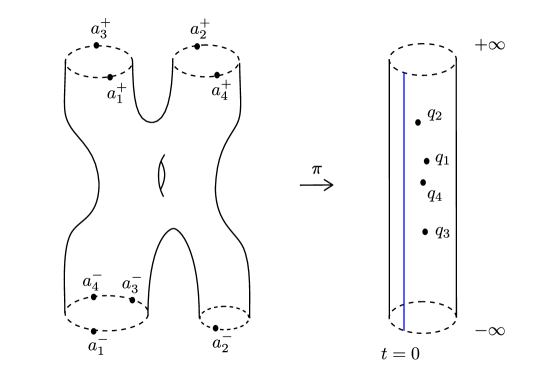
Figure 3. A sample element of $\mathcal{H}^{(2,2),(3,1)}_{4,-4}$.

Remark 2.14.

Notice that given a geometric branched cover $\pi\colon S\rightarrow\mathbb{R}\times S^{1}$ for each puncture $p_{i}^{+}$ (resp. $p_{i}^{-}$) there are only $\mu_{i}$ (resp. $\mu_{i}^{\prime}$) possible choices for the marker $a_{i}^{+}$ (resp. $a_{i}^{-}$).

Recall that $\text{Aut}_{v}(\mathbb{R}\times S^{1})\cong\mathbb{R}$ is a group of vertical translations on the standard cylinder. This group induces an $\mathbb{R}$-action on $\widetilde{\mathcal{H}}^{\bm{\mu},\bm{\mu}^{\prime}}_{\kappa,\chi}$ by translating the target of a given branched cover. We denote by $\mathcal{H}^{\bm{\mu},\bm{\mu}^{\prime}}_{\kappa,\chi}$ the quotient space by this action.

Remark 2.15.

Note that to get the standard Hurwitz scheme $\accentset{\circ}{\mathcal{H}}^{\bm{\mu},\bm{\mu}^{\prime}}_{\kappa,\chi}$ as defined in [Ful69] or alternatively in a more analytic setting in [Ion02] one has to drop the asymptotic marker data and take a quotient by the action of the whole group $\text{Aut}(\mathbb{R}\times S^{1})$ containing $\text{Aut}_{v}(\mathbb{R}\times S^{1})$ as its subgroup.

Definition 2.16.

A branched cover building

$$\left(\bm{C},S=S_{1}\cup\ldots\cup S_{n},\pi,(\bm{v}^{1},\ldots,\bm{v}^{n-1}),(\bm{m}^{1},\ldots,\bm{m}^{n-1})\right),$$

with Euler characteristic $\chi$ and profile $(\bm{\mu},\bm{\mu}^{\prime})$ consists of the following data:

1. A cylindrical building $\bm{C}=(\overrightarrow{C}=(C_{1},\ldots,C_{n}),j,(q_{1},\ldots,q_{b}),D))\in\overline{\mathcal{C}}_{b}$.

2. A punctured nodal Riemann surface $S$ decomposed as $S=S_{1}\cup\ldots\cup S_{n}$ with punctures at $\bm{p}^{+},\bm{p}^{-}$, a marked collection of special nodes

   $$v^{1}_{1},\ldots,v^{1}_{\ell_{1}},v^{2}_{1},\ldots,v^{2}_{\ell_{2}},v^{3}_{1},\ldots,v^{n-1}_{1},\ldots,v^{n-1}_{\ell_{n-1}}$$

   and maybe some other nodes. We require that $S_{i}\cap S_{i+1}=\{v^{i}_{1},\ldots,v^{i}_{l_{i}}\}=\bm{v}^{i}$; writing each node as $v^{i}_{j}=(v^{i}_{j,+},v^{i}_{j,-})$, we use the convention that $v^{i}_{j,+}\in S_{i+1}$ and $v^{i}_{j,-}\in S_{i}$. We regard each tuple $\bm{v}^{i}$ as an unordered collection of nodes and the lower indices above are used here to simplify the notation.

3. An admissible cover $\pi\colon S\longrightarrow\bm{C}$ , i.e., a branched cover that is simply branched at $q_{1},\ldots,q_{b}$, has a branching profile $\bm{\mu}$ at $+\infty_{1}$ (by which we mean $+\infty$ of the $C_{1}$ level of $\bm{C}$) and a branching profile $\bm{\mu}^{\prime}$ at $-\infty_{n}$ and is possibly branched at nodes. It is required that $\pi^{-1}(C_{i})=S_{i}$ and that the preimage of a node $\{-\infty_{i},+\infty_{i+1}\}$ under $\pi$ is given by $S_{i}\cap S_{i+1}$. The covering $\pi$ has the same degree when restricted to each of the $S_{i}$.

4. For each positive puncture $p_{i}^{+}$ (resp. negative puncture $p_{i}^{-}$) an asymptotic marker $a_{i}^{+}\in\mathcal{S}^{1}_{p_{i}^{+}}S=(T_{p_{i}^{+}}\overline{S}\setminus\{0\})/\mathbb{R}_{>0}$ (resp. an asymptotic marker $a_{i}^{-}\in\mathcal{S}^{1}_{p_{i}^{-}}S$), satisfying that $\pi_{*}(a_{i}^{+})=1\in\mathcal{S}^{1}_{+\infty}\overline{C_{1}}$ (resp. $\pi_{*}(a_{i}^{-})=1\in\mathcal{S}^{1}_{-\infty}\overline{C_{n}}$).

5. For each of the nodes $v^{i}_{j}$ as above, there is an assigned matching marker given by the choice of $m^{i}_{j}\in\mathcal{S}^{1}_{v^{i}_{j}}S$ such that it is mapped to

   $$1\in\mathcal{S}^{1}_{q_{-\infty}^{i},q_{+\infty}^{i+1}}\bm{C}=(T_{q_{-\infty}^{i}}C_{i}\otimes T_{q_{+\infty}^{i+1}}C_{i+1}\setminus 0)/\mathbb{R}_{>0}$$

   under the following composition (see (2.42) and (2.44) for the notation that we use here)

   Here $e_{\pi}(v^{i}_{j})$ is the ramification index of $\pi$ at the node $v^{i}_{j}$ and the map $\pi_{*}$ is induced by natural maps linear associated with $\pi$:

   $$(T_{v_{j,-}^{i}}S_{i+1})^{\otimes e_{\pi}(v^{i}_{j})}\to T_{q_{-\infty}^{i}}C_{i},$$

   $$(T_{v_{j,+}^{i}}S_{i})^{\otimes e_{\pi}(v^{i}_{j})}\to T_{q_{+\infty}^{i+1}}C_{i+1}.$$

   We refer the reader to (2.41), (2.42) and (2.44) for the notation we use here. We point out that the horizontal arrow in the diagram above is nothing but an $e_{\pi}(v^{i}_{j})$-sheeted cover of a circle by another circle and that $\pi_{*}$ is a diffeomorphism. We will denote the tuple of matching markers corresponding to the tuple of nodes $\bm{v}^{i}$ “connecting” $S_{i}$ and $S_{i+1}$ by $\bm{m}^{i}$.

Two branched cover buildings

$$\left(\bm{C},S=S_{1}\cup\ldots\cup S_{n},\pi,(\bm{v}^{1},\ldots,\bm{v}^{n-1}),(\bm{m}^{1},\ldots,\bm{m}^{n-1})\right),$$

$$\left(\bm{C}^{\prime},S^{\prime}=S_{1}^{\prime}\cup\ldots\cup S_{n}^{\prime},\pi^{\prime},(\bm{v}^{\prime 1},\ldots,\bm{v}^{\prime n-1}),(\bm{m}^{\prime 1},\ldots,\bm{m}^{\prime n-1})\right)$$

are isomorphic if there exists a pair $(\bm{\alpha}\colon S\rightarrow S^{\prime},\bm{\beta})$ with $\bm{\alpha}$ consisting of biholomorphisms $\alpha_{i}\colon S_{i}\rightarrow S_{i}^{\prime}$ and $\bm{\beta}\in\text{Aut}_{v}(\bm{C})$ (see Section 2.4) is a collection consisting of $\beta_{i}\in\text{Aut}_{v}(C_{i})$, satisfying:

1. $\alpha_{1}(p^{+}_{i})=p_{i}^{\prime+}$, $\alpha_{n}(p^{-}_{i})=p_{i}^{\prime-}$;

2. $\alpha_{1}(a^{+}_{i})=a_{i}^{\prime+}$, $\alpha_{n}(a^{-}_{i})=a_{n}^{\prime-}$;

3. $\bm{\alpha}(\bm{v}^{i})=\bm{v}^{\prime i}$ as unordered tuples; given some orderings on $\bm{v}^{i}$ and $\bm{v}^{\prime i}$ we denote by $j(\bm{\alpha})$ some index satisfying $\bm{\alpha}(v^{i}_{j})=v^{\prime i}_{j(\bm{\alpha})}$;

4. for the orderings as above $\bm{\alpha}^{i}_{*}(m^{i}_{j})=m^{\prime i}_{j(\bm{\alpha})}$, where $\alpha^{i}_{*}$ is the induced diffeomorphism

   $$\alpha^{i}_{*}\colon\mathcal{S}^{1}_{v^{i}_{j}}S\to\mathcal{S}^{1}_{v^{\prime i}_{j(\bm{\alpha})}}S^{\prime};$$

5. $\bm{\beta}(q_{j})=q_{j}^{\prime}$ and $\bm{\beta}\circ\pi^{\prime}\circ\bm{\alpha}=\pi$.

We stress that in the definition above the tuples $\bm{v}^{i}=\{v^{i}_{1},\ldots v^{i}_{l_{i}}\}$ are unordered (i.e., reordering these collections in the definition above does not change the class of a branched cover building).

Remark 2.17.

A matching marker as above can be interpreted as a choice of gluing between two cylindrical ends corresponding to a given node.

We denote by $\overline{\mathcal{H}}^{\bm{\mu},\bm{\mu}^{\prime}}_{\kappa,\chi}$ the set of all branched cover buildings.

Definition 2.18.

Let $\widehat{\mathcal{H}}^{\bm{\mu},\bm{\mu}^{\prime}}_{\kappa,\chi}$ be the subset of $\overline{\mathcal{H}}^{\bm{\mu},\bm{\mu}^{\prime}}_{\kappa,\chi}$ consisting of branched cover buildings with smooth levels by which we mean those branched cover buildings

$$\left(\bm{C},S=S_{1}\cup\ldots\cup S_{n},\pi,(\bm{v}^{1},\ldots,\bm{v}^{n-1}),(\bm{m}^{1},\ldots,\bm{m}^{n-1})\right)$$

for which the only nodes of $S$ are the special nodes connecting different levels, i.e., those nodes which are contained in the tuples $(\bm{v}^{1},\ldots,\bm{v}^{n-1})$.

Remark 2.19.

As per Remark 2.8, the space of branched cover buildings with smooth levels $\widehat{\mathcal{H}}^{\bm{\mu},\bm{\mu}^{\prime}}_{\kappa,\chi}$ is of main interest to us as we will be able to show that it is enough to consider only such types of domains for moduli spaces of pseudo-holomorphic curves involved in the definition of Heegaard Floer symplectic cohomology; see Theorem 2.38 for details.

We now discuss the relationship between Harris-Mumford compactification via admissible covers $\accentset{\circ}{\overline{\mathcal{H}}}^{\bm{\mu},\bm{\mu}^{\prime}}_{\kappa,\chi}$ and $\overline{\mathcal{H}}^{\bm{\mu},\bm{\mu}^{\prime}}_{\kappa,\chi}$, continuing the discussion in Remarks 2.10 and 2.15. In particular, we give a more precise description of the role of the matching data.

As mentioned in Remark 2.15 there is a fiber bundle

(2.45) $$\mathcal{H}^{\bm{\mu},\bm{\mu}^{\prime}}_{\kappa,\chi}\to\accentset{\circ}{\mathcal{H}}^{\bm{\mu},\bm{\mu}^{\prime}}_{\kappa,\chi}.$$

We claim that this map extends to

(2.46) $$\overline{\mathcal{H}}^{\bm{\mu},\bm{\mu}^{\prime}}_{\kappa,\chi}\to\accentset{\circ}{\overline{\mathcal{H}}}^{\bm{\mu},\bm{\mu}^{\prime}}_{\kappa,\chi}$$

and fits into the diagram

As in the case of the Hurwitz scheme, there is a map

(2.47) $$\mathcal{H}^{\bm{\mu},\bm{\mu}^{\prime}}_{\kappa,\chi}\to\overline{\mathcal{M}}_{\chi,\ell(\bm{\mu})+\ell(\bm{\mu}^{\prime})},$$

defined by taking the domain of a branched cover. Here $\overline{\mathcal{M}}_{\chi,\ell(\bm{\mu})+\ell(\bm{\mu}^{\prime})}$ is the moduli space of nodal, possibly disconnected curves of Euler characteristic $\chi$ with $\ell(\bm{\mu})+\ell(\bm{\mu}^{\prime})$ marked points (recall that $\ell(\bm{\mu})$ refers to the length of the partition $\bm{\mu}$).

Given two nodal curves $C_{1}$ and $C_{2}$ with $n_{1}+k$ and $n_{2}+k$ marked points one may produce a new curve $C$ by taking the disjoint union of $C_{1}$ and $C_{2}$ and identifying the last $k$ marked points of both curves. This construction induces the attaching map

(2.48) $$\overline{\mathcal{M}}_{\chi_{1},n_{1}+k}\times\overline{\mathcal{M}}_{\chi_{2},n_{2}+k}\longrightarrow\overline{\mathcal{M}}_{\chi_{1}+\chi_{2},n_{1}+n_{2}}.$$

The attaching map gives rise to the description of boundary strata for both $\overline{\mathcal{H}}^{\bm{\mu},\bm{\mu}^{\prime}}_{\kappa,\chi}$ and $\accentset{\circ}{\overline{\mathcal{H}}}^{\bm{\mu},\bm{\mu}^{\prime}}_{\kappa,\chi}$ which arises from the following diagram (we draw the diagram only for $\overline{\mathcal{H}}^{\bm{\mu},\bm{\mu}^{\prime}}_{\kappa,\chi}$)

(2.49)

The maps induced by the attaching map fit into the following commutative diagram

Note that to define a map given by the arrow in the top row of the diagram above one has to assign matching data based on asymptotic markers at punctures corresponding to $\bm{\mu}^{\prime\prime}$-profiles, unlike the arrow in the bottom row where all this data is not present.

Definition 2.20.

We define

(2.50) $${\mathcal{H}^{\bm{\mu},\bm{\mu}^{\prime\prime}}_{\kappa,\chi_{1}}\times_{\bm{m}}\mathcal{H}^{\bm{\mu}^{\prime\prime},\bm{\mu}^{\prime}}_{\kappa,\chi_{2}}}\subset\partial\overline{\mathcal{H}}^{\bm{\mu},\bm{\mu}^{\prime}}_{\kappa,\chi}$$

to be the part of $\widehat{\mathcal{H}}^{\bm{\mu},\bm{\mu}^{\prime}}_{\kappa,\chi}$ consisting of branched cover buildings with smooth levels of height $2$

$$\left(\bm{C}=(C_{1},C_{2}),S=S_{1}\cup S_{2},\pi,\bm{v}=\{v_{1}^{1},\ldots,v^{1}_{\ell(\bm{\mu}^{\prime\prime})}\},\bm{m}=\{m_{1}^{1},\ldots,m_{\ell(\bm{\mu}^{\prime\prime})}^{1}\}\right)$$

with:

• $\chi(S_{1})=\chi_{1}$, $\chi(S_{2})=\chi_{2}$ and $\chi=\chi_{1}+\chi_{2}$;

• ramification indices of $\pi$ at nodes $\bm{v}$ constituting a partition $\bm{\mu}^{\prime\prime}$ which appears in the notation (2.50).

We point out that an element of $\mathcal{H}^{\bm{\mu},\bm{\mu}^{\prime\prime}}_{\kappa,\chi_{1}}\times_{\bm{m}}\mathcal{H}^{\bm{\mu}^{\prime\prime},\bm{\mu}^{\prime}}_{\kappa,\chi_{2}}$, unlike an element of the direct product $\mathcal{H}^{\bm{\mu},\bm{\mu}^{\prime\prime}}_{\kappa,\chi_{1}}\times\mathcal{H}^{\bm{\mu}^{\prime\prime},\bm{\mu}^{\prime}}_{\kappa,\chi_{2}}$, possesses a choice of asymptotic markers at nodes corresponding to cylindrical ends with assigned partition $\bm{\mu}^{\prime\prime}$, i.e. to the nodes $\bm{v}$. On the contrary, there is a natural “forgetful” covering

(2.51) $$bf^{1}\colon\mathcal{H}^{\bm{\mu},\bm{\mu}^{\prime\prime}}_{\kappa,\chi_{1}}\times\mathcal{H}^{\bm{\mu}^{\prime\prime},\bm{\mu}^{\prime}}_{\kappa,\chi_{2}}\to\mathcal{H}^{\bm{\mu},\bm{\mu}^{\prime\prime}}_{\kappa,\chi_{1}}\times_{\bm{m}}\mathcal{H}^{\bm{\mu}^{\prime\prime},\bm{\mu}^{\prime}}_{\kappa,\chi_{2}}$$

given by matching the negative asymptotic markers of a given element of $\mathcal{H}^{\bm{\mu},\bm{\mu}^{\prime\prime}}_{\kappa,\chi_{1}}$ with corresponding (via the order on punctures) positive asymptotic markers of $\mathcal{H}^{\bm{\mu},\bm{\mu}^{\prime\prime}}_{\kappa,\chi_{2}}$ and forgetting these two sets of asymptotic markers. Explicitly, given a pair

(2.52) $$\left((S_{1},\pi_{1},\bm{p}^{\pm}_{1},\bm{a}^{\pm}_{1},B_{1}),(S_{2},\pi_{2},\bm{p}^{\pm}_{2},\bm{a}^{\pm}_{2},B_{2})\right)\in\mathcal{H}^{\bm{\mu},\bm{\mu}^{\prime\prime}}_{\kappa,\chi_{1}}\times\mathcal{H}^{\bm{\mu}^{\prime\prime},\bm{\mu}^{\prime}}_{\kappa,\chi_{2}}$$

We set $\bm{C}$ to be simply a union of two cylinders $C_{1}$ and $C_{2}$ with one special node. Further, we set $S$ to be the union of $S_{1}$ and $S_{2}$ glued along pairs of punctures $v^{1}_{i}=\{p^{-}_{1i},p^{+}_{2i}\}$. To each such pair, we associate a matching marker

(2.53) $$m^{1}_{i}=a^{-}_{1i}\otimes a^{+}_{2i}\in\mathcal{S}^{1}_{\{p^{-}_{1i},p^{+}_{2i}\}}S=(T_{p_{1i}^{-}}\overline{S_{1}}\otimes T_{p_{2i}^{+}}\overline{S_{2}}\setminus\{0\})/\mathbb{R}.$$

Then the map (2.51) sends a pair as in (2.52) to

$$(\bm{C}=(C_{1},C_{2}),S=S_{1}\cup S_{2},\pi=\pi_{1}\cup_{\bm{v}}\pi_{2},\bm{v}=\{v^{1}_{1},\ldots,v^{1}_{\ell(\bm{\mu}^{\prime\prime})}\},\bm{m}=\{m^{1}_{1},\ldots,m^{1}_{\ell(\bm{\mu}^{\prime\prime})}\}).$$

Essentially, the subspace $\mathcal{H}^{\bm{\mu},\bm{\mu}^{\prime\prime}}_{\kappa,\chi_{1}}\times_{\bm{m}}\mathcal{H}^{\bm{\mu}^{\prime\prime},\bm{\mu}^{\prime}}_{\kappa,\chi_{2}}\subset\overline{\mathcal{H}}^{\bm{\mu},\bm{\mu}^{\prime}}_{\kappa,\chi}$ is the image of $\mathcal{H}^{\bm{\mu},\bm{\mu}^{\prime\prime}}_{\kappa,\chi_{1}}\times\mathcal{H}^{\bm{\mu}^{\prime\prime},\bm{\mu}^{\prime}}_{\kappa,\chi_{2}}$ under the top row map in the diagram (2.49). It is evident that this forgetful map is an $N_{\bm{\mu}^{\prime\prime}}$-sheeted covering (see (2.3)). The reason for this is that for any matching $m_{i}^{1}$ there are $\mu^{\prime\prime}_{i}$ pairs of asymptotic markers that are sent to $m^{1}_{i}$ under (2.53) and there are $R_{\bm{\mu}^{\prime\prime}}$ way to give an order on the nodes of an element of $\mathcal{H}^{\bm{\mu},\bm{\mu}^{\prime\prime}}_{\kappa,\chi_{1}}\times_{\bm{m}}\mathcal{H}^{\bm{\mu}^{\prime\prime},\bm{\mu}^{\prime}}_{\kappa,\chi_{2}}$.

Similarly, for the space of branched cover buildings with smooth levels of height $n$

$$\mathcal{H}^{\bm{\mu},\bm{\mu}_{1}^{\prime\prime}}_{\kappa,\chi_{1}}\times_{\bm{m}^{1}}\ldots\times_{\bm{m}^{n-1}}\mathcal{H}^{\bm{\mu}_{n}^{\prime\prime},\bm{\mu}^{\prime}}_{\kappa,\chi_{n}},$$

defined in a similar fashion to Definition 2.20, there is forgetful covering

(2.54) $$bf^{n-1}\colon\mathcal{H}^{\bm{\mu},\bm{\mu}_{1}^{\prime\prime}}_{\kappa,\chi_{1}}\times\ldots\times\mathcal{H}^{\bm{\mu}_{n}^{\prime\prime},\bm{\mu}^{\prime}}_{\kappa,\chi_{n}}\to\mathcal{H}^{\bm{\mu},\bm{\mu}_{1}^{\prime\prime}}_{\kappa,\chi_{1}}\times_{\bm{m}^{1}}\ldots\times_{\bm{m}^{n-1}}\mathcal{H}^{\bm{\mu}_{n}^{\prime\prime},\bm{\mu}^{\prime}}_{\kappa,\chi_{n}}$$

of degree $N_{\bm{\mu}_{1}^{\prime\prime}}\cdot\ldots\cdot N_{\bm{\mu}_{n}^{\prime\prime}}$.

We now give an interpretation of the matchings in terms of local deformations following [Ion02]. In particular, we claim that the neighborhood of the image of $\mathcal{H}^{\bm{\mu},\bm{\mu}^{\prime\prime}}_{\kappa,\chi_{1}}\times\mathcal{H}^{\bm{\mu}^{\prime\prime},\bm{\mu}^{\prime}}_{\kappa,\chi_{2}}$ is smooth.

We pick some element

(2.55) $$\left(\left(\pi_{1}\colon S_{1}\to C_{1}\right),\left(\pi_{2}\colon S_{2}\to C_{2}\right)\right)\in\mathcal{H}_{\kappa,\chi_{1}}^{\mu,\mu^{\prime\prime}}\times_{\bm{m}}\mathcal{H}_{\kappa,\chi_{2}}^{\mu^{\prime\prime},\mu^{\prime}}.$$

Recall that the normal bundle to the boundary stratum containing $(S_{1},S_{2})\in\overline{\mathcal{M}}_{\chi,\ell(\mu)+\ell(\mu^{\prime})}$ given by

(2.56) $$\bigoplus_{i=1}^{\ell(\mu^{\prime\prime})}L^{*}_{p_{1,i}^{-}}\otimes L^{*}_{p_{2,i}^{+}}$$

at this point has fiber

(2.57) $$\bigoplus_{i=1}^{\ell(\mu^{\prime\prime})}T_{p_{1,i}^{-}}S_{1}\otimes T_{p_{2,i}^{+}}S_{2}.$$

A section of $L^{*}_{q_{-\infty}}\otimes L^{*}_{\tilde{q}_{+\infty}}$ given by $\zeta\in T_{q_{-}\infty}C_{1}\otimes T_{q_{+}\infty}C_{2}$ sets a restriction on sections of (2.56) which give rise to the deformation of the point (2.55) regarded as a point of $\accentset{\circ}{\overline{\mathcal{H}}}^{\bm{\mu},\bm{\mu}^{\prime}}_{\kappa,\chi}$ as shown in [Ion02]. More specifically, such a section given by

$$(\xi_{1},\ldots,\xi_{\ell(\mu^{\prime\prime})})\in\bigoplus_{i=1}^{\ell(\mu^{\prime\prime})}T_{p_{1,i}^{-}}S_{1}\otimes T_{p_{2,i}^{+}}S_{2}$$

has to satisfy

(2.58) $$\zeta=a_{1}\xi_{1}^{\mu^{\prime\prime}_{1}}=\ldots=a_{\ell(\mu^{\prime\prime})}\xi^{\mu^{\prime\prime}_{\ell(\mu^{\prime\prime})}}_{\ell(\mu^{\prime\prime})},$$

where $a_{1},\ldots,a_{\ell(\bm{\mu}^{\prime\prime})}\in\mathbb{C}$. We now recall that in the context of $\overline{\mathcal{H}}^{\bm{\mu},\bm{\mu}^{\prime}}_{\kappa,\chi}$ the section $\tilde{\zeta}$ as in (2.38) giving rise to local perturbation of $(C_{1},C_{2})\in\mathcal{C}_{b,2}$ has to satisfy $\varphi(\tilde{\zeta})=0$. We then claim that a section of (2.56) produces a point of $\mathcal{H}^{\bm{\mu},\bm{\mu}^{\prime}}_{\kappa,\chi}$ near (2.55) whenever

(2.59) $$\tilde{\zeta}=a_{1}\xi_{1}^{\mu^{\prime\prime}_{1}}=\ldots=a_{\ell(\mu^{\prime\prime})}\xi^{\mu^{\prime\prime}_{\ell(\mu^{\prime\prime})}}_{\ell(\mu^{\prime\prime})}.$$

At last, we claim that given a matching marker $m^{1}_{j}$ as in Definition 2.20 there is a unique choice of $\xi_{j}$ satisfying (2.59) with $[\xi_{j}]=m^{1}_{j}$ in $\mathcal{S}^{1}_{v^{i}_{j}}S$.

Hence, the coordinate chart (2.37) (and, moreover, the chart (2.40)) near the boundary of the space of cylindrical buildings gives lifts to coordinate charts near the corresponding portions of the boundary of $\overline{\mathcal{H}}^{\bm{\mu},\bm{\mu}^{\prime}}_{\kappa,\chi}$.

Notice that ${\mathcal{H}^{\bm{\mu},\bm{\mu}^{\prime\prime}}_{\kappa,\chi_{1}}\times_{\bm{m}}\mathcal{H}}^{\bm{\mu}^{\prime\prime},\bm{\mu}^{\prime}}_{\kappa,\chi_{2}}$ is a smooth manifold, as there are no non-trivial automorphisms of a curve fixing a marked point and an asymptotic marker at this point.

We conclude this discussion with the following theorem and refer the reader to [HM82, Moc95, Ion02] for further details.

Theorem 2.21.

The space $\overline{\mathcal{H}}^{\bm{\mu},\bm{\mu}^{\prime}}_{\kappa,\chi}$ is a compact metric space and serves as a compactification of the space $\mathcal{H}^{\bm{\mu},\bm{\mu}^{\prime}}_{\kappa,\chi}$, i.e., it coincides with the closure of $\mathcal{H}^{\bm{\mu},\bm{\mu}^{\prime}}_{\kappa,\chi}$ viewed as a subspace of $\overline{\mathcal{H}}^{\bm{\mu},\bm{\mu}^{\prime}}_{\kappa,\chi}$. Moreover, there is a smooth normal neighborhood near the space of height $2$ buildings with smooth levels

$$\mathcal{H}^{\bm{\mu},\bm{\mu}^{\prime\prime}}_{\kappa,\chi_{1}}\times_{\bm{m}}\mathcal{H}^{\bm{\mu}^{\prime\prime},\bm{\mu}^{\prime}}_{\kappa,\chi_{2}}\subset\overline{\mathcal{H}}^{\bm{\mu},\bm{\mu}^{\prime}}_{\kappa,\chi}$$

diffeomorphic to

(2.60) $$\mathcal{H}^{\bm{\mu},\bm{\mu}^{\prime\prime}}_{\kappa,\chi_{1}}\times_{\bm{m}}\mathcal{H}^{\bm{\mu}^{\prime\prime},\bm{\mu}^{\prime}}_{\kappa,\chi_{2}}\times[0,+\infty].$$

More generally, there is a normal neighborhood of

$$\mathcal{H}^{\bm{\mu},\bm{\mu}_{1}^{\prime\prime}}_{\kappa,\chi_{1}}\times_{\bm{m}^{1}}\ldots\times_{\bm{m}^{n-1}}\mathcal{H}^{\bm{\mu}_{n}^{\prime\prime},\bm{\mu}^{\prime}}_{\kappa,\chi_{n}}\subset\overline{\mathcal{H}}^{\bm{\mu},\bm{\mu}^{\prime}}_{\kappa,\chi}$$

diffeomorphic to

(2.61) $$\mathcal{H}^{\bm{\mu},\bm{\mu}_{1}^{\prime\prime}}_{\kappa,\chi_{1}}\times_{\bm{m}^{1}}\ldots\times_{\bm{m}^{n-1}}\mathcal{H}^{\bm{\mu}_{n}^{\prime\prime},\bm{\mu}^{\prime}}_{\kappa,\chi_{n}}\times[0,+\infty]^{n-1}.$$

Remark 2.22.

We note that the whole $\overline{\mathcal{H}}^{\bm{\mu},\bm{\mu}^{\prime}}_{\kappa,\chi}$ is not a manifold with corners or even an orbifold since there may be non-special nodes corresponding to bubbles on the cylindrical side. Nevertheless, the choice of matching data allows us to get a smooth structure on the preimage of smooth cylinders $\widetilde{C}_{-\chi}$. Recall that in the algebraic setting to get a smooth stack serving as compactification of $\accentset{\circ}{\mathcal{H}}^{\bm{\mu},\bm{\mu}^{\prime}}_{\kappa,\chi}$ one should add twisted covers as introduced in [ACV03] and more generally in [Deo14]. Working with $\overline{\mathcal{C}}_{-\chi}$ instead of $\overline{\mathcal{M}}_{0,\chi+2}$ allows us to avoid introducing “stacky” covers.

We will refer to $[0,+\infty]^{n-1}$ part in (2.61) as neck coordinates. For further use, we also discuss orientations on Hurwitz spaces. Any space $\widetilde{\mathcal{H}}^{\bm{\mu},\bm{\mu}^{\prime}}_{\kappa,\chi}$ is naturally oriented as it is a cover space over $\text{Conf}_{-\chi}(\mathbb{C}\setminus\{0,\infty\})$ which is a complex manifold. The choice of vertical direction $\partial_{s}$ leads to a further natural choice of orientation on $\mathcal{H}^{\bm{\mu},\bm{\mu}^{\prime}}_{\kappa,\chi}$. We fix such choices on all spaces $\mathcal{H}^{\bm{\mu},\bm{\mu}^{\prime}}_{\kappa,\chi}$.

We then claim that boundary orientation on the image of ${\mathcal{H}}^{\bm{\mu},\bm{\mu}^{\prime\prime}}_{\kappa,\chi_{1}}\times\mathcal{H}^{\bm{\mu}^{\prime\prime},\bm{\mu}^{\prime}}_{\kappa,\chi_{2}}$ under the map described in (2.49) coincides with the product orientation. In other words, there is a natural isomorphism

(2.62) $$|v|\otimes|{\mathcal{H}}^{\bm{\mu},\bm{\mu}^{\prime\prime}}_{\kappa,\chi_{1}}|\otimes|\mathcal{H}^{\bm{\mu}^{\prime\prime},\bm{\mu}^{\prime}}_{\kappa,\chi_{2}}|\cong|\mathcal{H}^{\bm{\mu},\bm{\mu}^{\prime}}_{\kappa,\chi}|$$

where $v$ is an outward pointing vector (corresponding to the normal direction described in (2.60)). Here we use conventions discussed in Section 2.14.

Remark 2.23.

We point out that assuming an order on the set of branched points as in the Definition 2.13 allows us to get a description of the portion of the boundary of $\mathcal{H}^{\bm{\mu},\bm{\mu}^{\prime}}_{\kappa,\chi}$ which is of interest to us. Nevertheless, in practice, it leads to “overcounting” geometric curves connecting tuples of Hamiltonian orbits. We ignore this disadvantage since Heegaard Floer symplectic cohomology is eventually defined over $\mathbb{Q}$. To eliminate this nuance one could use the approach of [Moc95] towards compactification of Hurwitz scheme with unordered branched points.

2.6. Review of branched manifolds

We start by reviewing the general framework of weighted nonsingular branched groupoids from [McD06].

Denote the spaces of objects and morphisms of a small topological category $\mathscr{X}$ by the letters $X_{0}$ and $X_{1}$ respectively. The source and target maps are denoted via $s,t\colon X_{1}\to X_{0}$, and the identity map is given by $x\mapsto\text{id}_{x}$ is $\operatorname{id}\colon X_{0}\to X_{1}$. The composition map is set as

$$m\colon{X_{1}}\;_{s}\!\times_{t}X_{1}\;\to\;X_{1},\quad(f,g)\mapsto f\circ g.$$

The space of morphisms from $x$ to $y$ is denoted by $\text{Hom}(x,y)$.

Definition 2.24.

A nonsingular (oriented) sse (smooth, stable, étale) groupoid with corners $\mathscr{X}$ is a small topological category such that the following conditions hold:

• (Groupoid) All morphisms are invertible, i.e., there is a structure map $\iota\colon X_{1}\to X_{1}$ that takes each $f\in X_{1}$ to its inverse $f^{-1}$.

• (Smooth) The spaces $X_{0}$ of objects and $X_{1}$ of morphisms are (oriented) manifolds with corners, and all structure maps ($s,t,m,\iota,\text{id}$) are smooth (and orientation-preserving).

• (Étale) If in addition to the above all structure maps are local diffeomorphisms.

• (Nonsingular) For each $x\in X_{0}$ the set of self-morphisms $\text{Hom}(x,x)\eqqcolon G_{x}$ is trivial (stability is a weaker condition which only requires finiteness of these groups).

We denote by $\mathscr{X}^{\vee}$ the quotient space of a small topological category groupoid $\mathscr{X}$ given by $X_{0}/\sim$, where $x\sim x^{\prime}$ if $\text{Hom}(x,x^{\prime})$ is non-empty. Denote by $\pi$ the projection $X_{0}\to\mathscr{X}^{\vee}$.

Further, we will simply call $\mathscr{X}$ a nonsingular sse groupoid if $X_{0}$ and $X_{1}$ are manifolds (without boundary or corners).

Let us recall that any topological space $Y$ admits a maximal Hausdorff quotient $(f,Y_{H})$, i.e., a projection $f\colon Y\to Y_{H}$ to a Hausdorff space $Y_{H}$, such that any other continuous surjection $f^{\prime}\colon Y\to Y^{\prime}$ with $Y^{\prime}$ Hausdorff factors through $f$.

For a given sse groupoid with boundary $\mathscr{B}$ denote by $\check{\pi}_{H}$ the projection $\mathscr{B}^{\vee}\to\mathscr{B}^{\vee}_{H}$ and by $\pi_{H}$ the projection $B_{0}\to\mathscr{B}^{\vee}_{H}$. Furthermore, $U_{H}=\pi_{H}(U)$ denotes the image of $U\subset B_{0}$ in $\mathscr{B}^{\vee}_{H}$.

Definition 2.25.

A weighted nonsingular branched groupoid with corners (or wnbc groupoid for short) is a pair $(\mathscr{B},\Lambda)$ consisting of an oriented, nonsingular sse groupoid with boundary together with a weighting function $\Lambda\colon\mathscr{B}^{\vee}_{H}\to(0,\infty)$ that satisfies the following compatibility conditions. For each $p\in\mathscr{B}^{\vee}_{H}$ there is an open neighborhood $N$ of $p$ in $\mathscr{B}^{\vee}_{H}$, a collection $U_{1},\ldots,U_{\ell}$ of disjoint open subsets of $\pi_{H}^{-1}(N)\subset B_{0}$ (called local branches) and a set of positive weights $m_{1},\ldots,m_{\ell}$ such that:

• $\check{\pi}_{H}^{-1}(N)=U_{1}^{\vee}\cup\ldots\cup U_{\ell}^{\vee}\subset\mathscr{B}^{\vee}$;

• for each $i=1,\ldots,\ell$ the projection $\pi_{H}\colon U_{i}\to(U_{i}^{\vee})_{H}$ is a homeomorphism onto a relatively closed subset of $N$;

• for all $q\in N$, $\Lambda(q)$ is the sum of the weights of the local branches whose image contains $q$:

  $$\Lambda(q)=\underset{i\colon q\in\,(U_{i}^{\vee})_{H}}{\sum}m_{i}.$$

We call $(\mathscr{B},\Lambda)$ a wnb groupoid if $\mathscr{B}$ is a nonsingular sse groupoid (i.e., with no boundary).

Later, we also use the notion of an orbibundle over a wnb groupoid $\rho\colon\mathscr{E}\to\mathscr{B}$. This can be thought of as a vector bundle $\rho_{0}\colon E_{0}\to B_{0}$ with $E_{1}$ representing identifications between fibers $E_{x}$ and $E_{y}$ for any $f\in\text{Hom}(x,y)$; see [McD06] for details. A section of such a bundle is a smooth functor $\sigma\colon\mathscr{B}\to\mathscr{E}$. A section $\sigma$ is said to be transverse to the zero section if $\sigma(B_{0})$ is transverse to the zero set of $E_{0}$ and $d\sigma\colon T_{x}\mathscr{B}\to E_{x}$ is surjective (here $T\mathscr{B}$ is the naturally defined tangent bundle of a wnb groupoid $\mathscr{B}$) for any intersection point $x\in B_{0}$. Notice that a structure of a wnb groupoid on $\mathscr{B}$ induces a structure of a wnb groupoid in the zero set $\mathscr{Z}(\sigma)$ for transversal $\sigma$.

2.7. Branched structure on Hurwitz spaces.

In this section, we define a wnbc groupoid $\widehat{\mathscr{H}}^{\bm{\mu},\bm{\mu}^{\prime}}_{\kappa,\chi}$ by means of an inductive procedure. The motivation behind the construction to follow is discussed in Section 2.8.

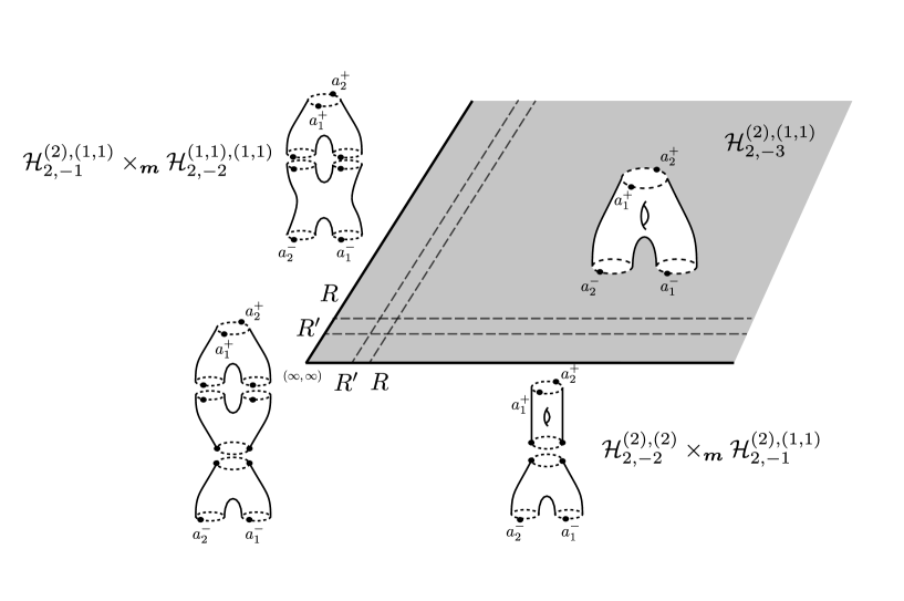
(a)

Figure 4. Here is a toy picture of $\overline{\mathcal{H}}^{(2),(1,1)}_{2,-3}$, i.e., we have $\kappa=2,\,\chi=-3,\,\bm{\mu}=(2),\,\bm{\mu}^{\prime}=(1,1)$, and the interior $\mathcal{H}^{(2),(1,1)}_{2,-3}$ is in gray. The black horizontal ray corresponds to a portion of the boundary associated with $\bm{\mu}^{\prime\prime}=(2)$ and the vertical ray corresponds to $\bm{\mu}^{\prime\prime}=(1,1)$. We also regard it as a cartoon for Step 0 in our construction.

Step $k=0$. We start with $(\mathscr{B},\Lambda)$, where $B_{0}=\mathcal{H}^{\bm{\mu},\bm{\mu}^{\prime}}_{\kappa,\chi}$, $B_{1}$ consists only of $\text{id}_{x}$ for $x\in B_{0}$ and $\Lambda\equiv 1$. Here, the convention is that $B_{0}$ denotes the objects of $\mathscr{B}$ and $B_{1}$ denotes its morphisms. We then modify $(\mathscr{B},\Lambda)$ in the next steps.

Step $k=1$: adding buildings of height $2$.

Recall that by Theorem 2.21 for any codimension-$1$ portion of the boundary $\partial\widehat{\mathcal{H}}^{\bm{\mu},\bm{\mu}^{\prime}}_{\kappa,\chi}$ consisting of smooth buildings of height $2$ of the form $\mathcal{H}^{\bm{\mu},\bm{\mu}^{\prime\prime}}_{\kappa,\chi_{1}}\times_{\bm{m}}\mathcal{H}^{\bm{\mu}^{\prime\prime},\bm{\mu}^{\prime}}_{\kappa,\chi_{2}}$ (for any pair $\chi_{1},\chi_{2}$ such that $\chi_{1}+\chi_{2}=\chi$) there is a neighborhood of the form

$$\mathcal{H}^{\bm{\mu},\bm{\mu}^{\prime\prime}}_{\kappa,\chi_{1}}\times_{\bm{m}}\mathcal{H}^{\bm{\mu}^{\prime\prime},\bm{\mu}^{\prime}}_{\kappa,\chi_{2}}\times(R;+\infty]$$

for any $R\geq 0$. We then introduce a “thickened” forgetful covering

(2.63) $$\overline{bf}^{1}\colon\mathcal{H}^{\bm{\mu},\bm{\mu}^{\prime\prime}}_{\kappa,\chi_{1}}\times\mathcal{H}^{\bm{\mu}^{\prime\prime},\bm{\mu}^{\prime}}_{\kappa,\chi_{2}}\times(R;+\infty]\to\mathcal{H}^{\bm{\mu},\bm{\mu}^{\prime\prime}}_{\kappa,\chi_{1}}\times_{\bm{m}}\mathcal{H}^{\bm{\mu}^{\prime\prime},\bm{\mu}^{\prime}}_{\kappa,\chi_{2}}\times(R;+\infty],$$

which is equal to $(bf^{1},\operatorname{Id})$. We also pick some $R^{\prime}>R$. Set

$$U_{0}=\mathcal{H}^{\bm{\mu},\bm{\mu}^{\prime}}_{\kappa,\chi}\setminus\bigcup_{\chi_{1}+\chi_{2}=\chi,\,\bm{\mu}^{\prime\prime}\vdash\kappa}\mathcal{H}^{\bm{\mu},\bm{\mu}^{\prime\prime}}_{\kappa,\chi_{1}}\times_{\bm{m}}\mathcal{H}^{\bm{\mu}^{\prime\prime},\bm{\mu}^{\prime}}_{\kappa,\chi_{2}}\times[R^{\prime};+\infty)$$

We update $(\mathscr{B},\Lambda)$ by putting

(2.64) $$B_{0}^{\text{new}}=U_{0}\sqcup\bigsqcup_{\chi_{1}+\chi_{2}=\chi,\,\bm{\mu}^{\prime\prime}\vdash\kappa}\mathcal{H}^{\bm{\mu},\bm{\mu}^{\prime\prime}}_{\kappa,\chi_{1}}\times\mathcal{H}^{\bm{\mu}^{\prime\prime},\bm{\mu}^{\prime}}_{\kappa,\chi_{2}}\times(R;+\infty].$$

We then set the manifold $B_{1}^{\text{new}}$ to record the following identifications corresponding to the thickened forgetful maps. Namely given a point $x\in\mathcal{H}^{\bm{\mu},\bm{\mu}^{\prime\prime}}_{\kappa,\chi_{1}}\times\mathcal{H}^{\bm{\mu}^{\prime\prime},\bm{\mu}^{\prime}}_{\kappa,\chi_{2}}\times(R;R^{\prime})\subset B_{0}$ we then set $\operatorname{Hom}(x,\overline{bf}^{1}(x))$ and $\operatorname{Hom}(\overline{bf}^{1}(x),x)$ each to consist of one arrow, and these arrows are meant to be inverses of one another. We then complete $B_{1}^{\text{new}}$ by adding all the necessary arrows to make it into a groupoid. The weight function $\Lambda^{\text{new}}$ is set to be equal to $1$ on the closure of $\pi_{H}^{\vee}(U_{0})$ and equal to $\frac{1}{N_{\bm{\mu}^{\prime\prime}}}$ on the image of $\mathcal{H}^{\bm{\mu},\bm{\mu}^{\prime\prime}}_{\kappa,\chi_{1}}\times\mathcal{H}^{\bm{\mu}^{\prime\prime},\bm{\mu}^{\prime}}_{\kappa,\chi_{2}}\times(R^{\prime};+\infty]$ under $\pi_{H}^{\vee}$ for any $\chi_{1}+\chi_{2}=\chi$ and $\bm{\mu}^{\prime\prime}\vdash\kappa$ (clearly all of these images are pairwise disjoint and all of them are disjoint from the closure of $\pi_{H}^{\vee}(U_{0})$). Evidently, the updated pair $(\mathscr{B}^{\text{new}},\Lambda^{\text{new}})$ is a wnbc groupoid.

Inductive step $k=n$: adding buildings of height $k+1$. In our construction, we obtain $B_{0}^{\text{new}}$ from $B_{0}^{\text{old}}$ (the one we got in step $k-1$) by truncating a portion of $B_{0}^{\text{old}}$ and adding a disjoint union of all possible “thickened” spaces of buildings of height $k+1$. Given that, let us consider

(2.65) $$\mathcal{H}^{\bm{\mu},\bm{\mu}^{\prime\prime}_{1}}_{\kappa,\chi_{1}}\times\ldots\times\mathcal{H}^{\bm{\mu}^{\prime\prime}_{k-1},\bm{\mu}^{\prime}}_{\kappa,\chi_{k}}\times(R;+\infty]^{k-1}\subset B_{0}^{\text{old}},\,\chi_{1}+\ldots+\chi_{k}=\chi.$$

Given $i$ such that $1\leq i\leq k$, $\bm{\mu}^{\prime\prime}\vdash\kappa$, and a pair $\chi_{i}^{\prime},\chi_{i}^{\prime\prime}$ such that $\chi_{i}^{\prime}+\chi_{i}^{\prime\prime}=\chi_{i}$, there is a subset of the above of the form

(2.66) $$\mathcal{H}^{\bm{\mu},\bm{\mu}^{\prime\prime}_{1}}_{\kappa,\chi_{1}}\times\ldots\times(\mathcal{H}^{\bm{\mu}^{\prime\prime}_{i},\bm{\mu}^{\prime\prime}}_{\kappa,\chi_{i}^{\prime}}\times_{\bm{m}}\mathcal{H}^{\bm{\mu}^{\prime\prime},\bm{\mu}^{\prime\prime}_{i+1}}_{\kappa,\chi_{i}^{\prime\prime}})\times\ldots\times\mathcal{H}^{\bm{\mu}^{\prime\prime}_{k-1},\bm{\mu}^{\prime}}_{\kappa,\chi_{k}}\times(R;+\infty)^{i-1}\times(R^{\prime};+\infty]\times(R;+\infty]^{k-i}$$

by Theorem 2.21. We then set $U_{0}$ to be equal to $B_{0}^{\text{old}}$ with subsets of type (2.66) subtracted from all the possible subsets of the form (2.65) in $B_{0}^{\text{old}}$. Furthermore, we put

(2.67) $$B_{0}^{\text{new}}=U_{0}\sqcup\bigsqcup_{\begin{subarray}{c}\chi_{1}+\ldots+\chi_{k+1}=\chi,\\ \bm{\mu}^{\prime\prime}_{1},\ldots,\bm{\mu}^{\prime\prime}_{k}\vdash\kappa\end{subarray}}\mathcal{H}^{\bm{\mu},\bm{\mu}^{\prime\prime}_{1}}_{\kappa,\chi_{1}}\times\ldots\times\mathcal{H}^{\bm{\mu}^{\prime\prime}_{k},\bm{\mu}^{\prime}}_{\kappa,\chi_{k+1}}\times(R;+\infty]^{k}$$

As in Step $1$ there are thickened forgetful maps

(2.68) $$\overline{bf}^{1}_{i}\colon\mathcal{H}^{\bm{\mu},\bm{\mu}^{\prime\prime}_{1}}_{\kappa,\chi_{1}}\times\ldots\times\mathcal{H}^{\bm{\mu}^{\prime\prime}_{k},\bm{\mu}^{\prime}}_{\kappa,\chi_{k+1}}\times(R;+\infty]^{i-1}\times(R,R^{\prime})\times(R,+\infty]^{k-i}\to$$

$$\mathcal{H}^{\bm{\mu},\bm{\mu}^{\prime\prime}_{1}}_{\kappa,\chi_{1}}\times\ldots\times(\mathcal{H}^{\bm{\mu}^{\prime\prime}_{i},\bm{\mu}^{\prime\prime}}_{\kappa,\chi_{i}^{\prime}}\times_{\bm{m}}\mathcal{H}^{\bm{\mu}^{\prime\prime},\bm{\mu}^{\prime\prime}_{i+1}}_{\kappa,\chi_{i}^{\prime\prime}})\times\ldots\times\mathcal{H}^{\bm{\mu}^{\prime\prime}_{k-1},\bm{\mu}^{\prime}}_{\kappa,\chi_{k}}\times(R;+\infty]^{i-1}\times(R,R^{\prime})\times(R;+\infty]^{k-i}$$

We set $B_{1}$ to track identifications between points with the same images under these maps. At last, $\Lambda^{\text{new}}$ is set to coincide with $\Lambda^{\text{old}}$ at the points of $U_{0}$ and is set to be equal to $\frac{1}{N_{\bm{\mu}^{\prime\prime}_{1}}\cdot\ldots\cdot N_{\bm{\mu}^{\prime\prime}_{k}}}$ on the portion of the image under $\pi_{H}^{\vee}$ of

(2.69) $$\mathcal{H}^{\bm{\mu},\bm{\mu}^{\prime\prime}_{1}}_{\kappa,\chi_{1}}\times\ldots\times\mathcal{H}^{\bm{\mu}^{\prime\prime}_{k},\bm{\mu}^{\prime}}_{\kappa,\chi_{k+1}}\times(R;+\infty]^{k}$$

disjoint from $\overline{\pi_{H}^{\vee}(U_{0})}\subset\mathscr{B}_{H}^{\vee}$.

The verification that the resulting $(\mathscr{B},\Lambda)$ is indeed a wnbc groupoid is straightforward.

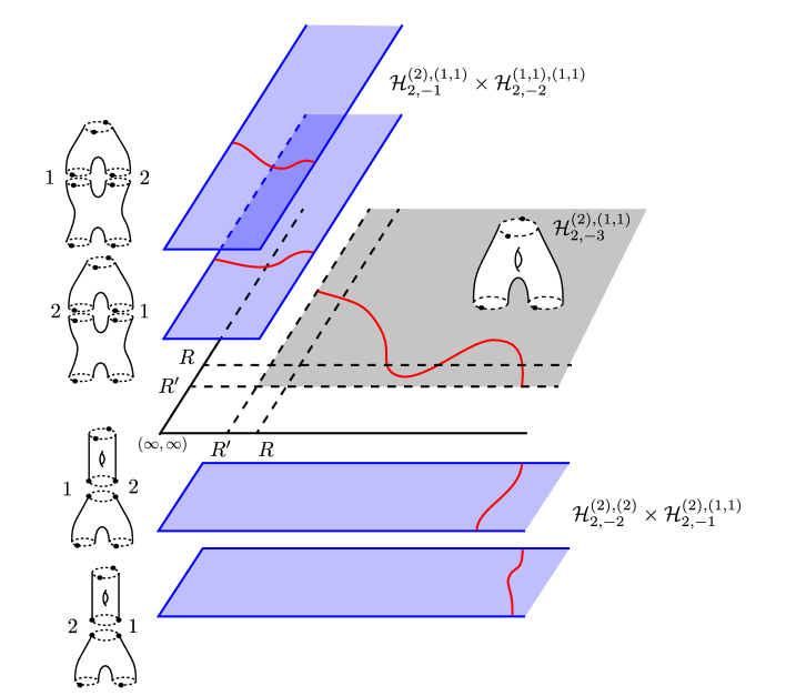
(a)

Figure 5. Step 1 of the construction of the wnbc groupoid $\widehat{\mathscr{H}}^{(2),(1,1)}_{2,-3}$ is shown here. For $\bm{\mu}^{\prime\prime}=(1,1)$ we have $N_{\bm{\mu}^{\prime\prime}}=2$ and it counts the number of ways to order a set of two orbits. For $\bm{\mu}^{\prime\prime}=(2)$ we have $N_{\bm{\mu}^{\prime\prime}}=2$ and it counts the number of ways to choose an asymptotic marker on a time-$2$ orbit. Therefore, the construction provides four boundary neighborhoods given in blue. The weight function takes the value $\Lambda=\frac{1}{2}$ in each of these regions. The red curves depict $\mathscr{M}^{-3}(H^{\text{tot}};J;\bm{x};\bm{x}^{\prime})$ for some $\bm{x},\bm{x}^{\prime}\in\mathcal{P}_{\text{psym}}$. In each of the blue regions, the Floer data introduced in Section 2.8 force the red projection to be slightly altered.

The wnbc groupoid obtained after the termination of the process above is further denoted by $(\widehat{\mathscr{H}}^{\bm{\mu},\bm{\mu}^{\prime}}_{\kappa,\chi},\Lambda_{\widehat{\mathscr{H}}^{\bm{\mu},\bm{\mu}^{\prime}}_{\kappa,\chi}})$. We denote the interior wnb groupoid (obtained by throwing out the boundary at the level of $B_{0}$) by $\mathscr{H}^{\bm{\mu},\bm{\mu}^{\prime}}_{\kappa,\chi}$.

There is a natural projection

(2.70) $$\mathscr{BF}\colon(\widehat{\mathscr{H}}^{\bm{\mu},\bm{\mu}^{\prime}}_{\kappa,\chi})^{\vee}\to\widehat{\mathcal{H}}^{\bm{\mu},\bm{\mu}^{\prime}}_{\kappa,\chi}$$

induced by forgetful maps. That is, for any $x\in(\widehat{\mathscr{H}}^{\bm{\mu},\bm{\mu}^{\prime}}_{\kappa,\chi})^{\vee}$ we may pick a maximal height $k$ such that $x$ belongs to a portion of

$$\mathcal{H}^{\bm{\mu},\bm{\mu}^{\prime\prime}_{1}}_{\kappa,\chi_{1}}\times\ldots\times\mathcal{H}^{\bm{\mu}^{\prime\prime}_{k},\bm{\mu}^{\prime}}_{\kappa,\chi_{k+1}}\times(R;+\infty]^{k}$$

left in our inductive construction and we then send $x$ to $bf^{k}(x)$. These locally defined maps clearly patch into a continuous map $\mathscr{BF}$.

We will use the notation $\widetilde{\mathscr{H}}^{\bm{\mu},\bm{\mu}^{\prime}}_{\kappa,\chi}$ to denote the branched structure on $\widetilde{\mathcal{H}}^{\bm{\mu},\bm{\mu}^{\prime}}_{\kappa,\chi}$ induced by $\mathscr{H}^{\bm{\mu},\bm{\mu}^{\prime}}_{\kappa,\chi}$.

Remark 2.26.

The reasoning for this construction is provided in the next section. Roughly speaking, for breaking of profile $\bm{\mu}^{\prime\prime}$ one might want to have not only matching data and a non-decreasing order of entries of $\bm{\mu}^{\prime\prime}$ but a choice of actual markers (there are $\bm{\mu}^{\prime\prime}!$ choices) and a total order on partition $\bm{\mu}^{\prime\prime}$ (there are $R_{\bm{\mu}^{\prime\prime}}$ such orders).

Remark 2.27.

We point out that this branched structure can be extended to the whole of $\overline{\mathcal{H}}^{\bm{\mu},\bm{\mu}^{\prime}}_{\kappa,\chi}$.

2.8. Floer data

For each $\mathcal{H}^{\bm{\mu},\bm{\mu}^{\prime}}_{\kappa,\chi}$ and all elements $(S,\pi,\bm{p}^{\pm},\bm{a}^{\pm},B)\in\widetilde{\mathcal{H}}^{\bm{\mu},\bm{\mu}^{\prime}}_{\kappa,\chi}$ we choose a cylindrical ends data on $S$ such that $\bm{p}^{+}$ is the set of inputs and $\bm{p}^{-}$ is the set of outputs, i.e., a collection of holomorphic embeddings $\{\delta^{i}_{+}\}_{i=1}^{i=\ell(\bm{\mu})}$ and $\{\delta^{i}_{-}\}_{i=1}^{i=\ell(\bm{\mu}^{\prime})}$ satisfying compatibility conditions that vary smoothly:

• $\delta_{+}^{i}\colon\mathbb{R}_{\geq R_{i}^{+}}\times\mathbb{R}/\mu_{i}\mathbb{Z}\to S,\,\lim\limits_{s\to+\infty}\delta_{+}^{i}(s,\cdot)=p_{i}^{+},\,\lim\limits_{s\to+\infty}-\frac{d}{ds}\delta_{+}^{i}(s,0)=a_{i}^{+};$

• compatibility with $\pi$: $\pi(\delta_{+}^{i}(s,t))=(s,t)$, where

  $$\pi\circ\delta_{+}^{i}\colon\mathbb{R}_{\geq R_{i}^{+}}\times\mathbb{R}/2\mu_{i}\pi\mathbb{Z}\to\mathbb{R}\times\mathbb{Z}/2\pi\mathbb{Z};$$

• $\delta_{-}^{i}\colon\mathbb{R}_{\leq-R_{i}^{-}}\times\mathbb{R}/\mu_{i}^{\prime}\mathbb{Z}\to S,\,\lim\limits_{s\to+\infty}\delta_{-}^{i}(s,\cdot)=p_{i}^{-},\,\lim\limits_{s\to-\infty}-\frac{d}{ds}\delta_{+}^{i}(s,0)=a_{i}^{-}$;

• compatibility with $\pi$: $\pi(\delta_{-}^{i}(s,t))=(s,t)$, where

  $$\pi\circ\delta_{+}^{i}\colon\mathbb{R}_{\leq-R_{i}^{-}}\times\mathbb{R}/\mu_{i}^{\prime}\mathbb{Z}\to\mathbb{R}\times\mathbb{Z}/2\pi\mathbb{Z}.$$

In particular, the constants $R_{i}^{+},R_{i}^{-}$ vary smoothly across $\widetilde{\mathcal{H}}^{\bm{\mu},\bm{\mu}^{\prime}}_{\kappa,\chi}$. It is required that the above choices are invariant under the $\mathbb{R}$-action on $\widetilde{\mathcal{H}}^{\bm{\mu},\bm{\mu}^{\prime}}_{\kappa,\chi}$ which provides a choice of cylindrical ends data on $\mathcal{H}^{\bm{\mu},\bm{\mu}^{\prime}}_{\kappa,\chi}$.

A choice of cylindrical ends data on $(\mathscr{H}^{\bm{\mu},\bm{\mu}^{\prime}}_{\kappa,\chi})^{\vee}_{H}$ is similar to the above; one has to choose such data on objects $\left(\mathscr{H}^{\bm{\mu},\bm{\mu}^{\prime}}_{\kappa,\chi}\right)_{0}$ making sure that it coincides for the pairs of points identified under morphisms $\left(\mathscr{H}^{\bm{\mu},\bm{\mu}^{\prime}}_{\kappa,\chi}\right)_{1}$. In particular, any cylindrical ends data on $\mathcal{H}^{\bm{\mu},\bm{\mu}^{\prime}}_{\kappa,\chi}$ provides cylindrical ends data on $\mathscr{H}^{\bm{\mu},\bm{\mu}^{\prime}}_{\kappa,\chi}$.

Now assume there are choices of cylindrical ends data for all $\mathcal{H}^{\bm{\mu},\bm{\mu}^{\prime}}_{\kappa,\chi^{\prime}}$ for all $\chi^{\prime}$ with $\chi^{\prime}>\chi$. Then we say that a choice of cylindrical end data is consistent if for any (see (2.67))

(2.71) $$([S=S_{1}\cup\ldots\cup S_{k+1},\pi],R_{1},\ldots,R_{k})\in\mathcal{H}^{\bm{\mu},\bm{\mu}^{\prime\prime}_{1}}_{\kappa,\chi_{1}}\times\ldots\times\mathcal{H}^{\bm{\mu}^{\prime\prime}_{k},\bm{\mu}^{\prime}}_{\kappa,\chi_{k+1}}\times(R;+\infty]^{k}\subset B_{0}$$

with $R_{1},\ldots,R_{k}\gg 0$ the cylindrical ends coincide with the ones induced from positive (resp. negative) ends of $S_{1}$ (resp. $S_{k+1}$).

Furthermore, for a point of $[S^{\prime},\pi^{\prime}]\in\widehat{\mathcal{H}}^{\bm{\mu},\bm{\mu}^{\prime}}_{\kappa,\chi}$ represented by (2.71) (by applying Theorem 2.21 to the image of (2.71) under the corresponding forgetful map $bf^{k}$) we may assign finite cylinders data. That is, the domain $S^{\prime}$ comes with $\ell(\bm{\mu}^{\prime\prime}_{j})$ necks of length $2R_{j}$ induced by the gluing procedure described in (2.36) and (2.59) for each $j$ with $1\leq j\leq k$.

Moreover, since $[S,\pi]$ above is the element of a product of Hurwitz spaces the cylindrical end data induces trivializations of portions of the necks as above. Namely, let $p^{i,-}_{j}$ be the $j$-th negative puncture of $S_{i}$ and $p^{i+1,+}_{j}$ be the $j$-th positive puncture of $S_{i+1}$. Both of the punctures come with associated cylindrical ends $\delta^{j}_{i,-}\colon\mathbb{R}_{\geq R^{i,-}_{j}}\times\mathbb{R}/\mu^{\prime\prime}_{ij}\mathbb{Z}\to S^{\prime}$ and $\delta^{j}_{i,+}\colon\mathbb{R}_{\leq R^{i,+}_{j}}\times\mathbb{R}/\mu^{\prime\prime}_{ij}\mathbb{Z}\to S^{\prime}$. Then under the gluing procedure dictated by the matching marker as in (2.53) a finite portion of $\delta^{j}_{i,-}$ is glued to a finite portion of $\delta^{j}_{i,+}$. This gives rise to a finite cylinder

• $\delta^{j}_{i,r}\colon[c_{r},d_{r}]\times\mathbb{R}/\mu^{\prime\prime}_{ij}\mathbb{Z}\to S$, which satisfies compatibility with $\pi^{\prime}$ up to a vertical translation.

We then say that a choice of finite cylinders and cylindrical ends on $\widehat{\mathscr{H}}^{\bm{\mu},\bm{\mu}^{\prime}}_{\kappa,\chi}$ is a consistent cylindrical data if for all points $[S,\pi]\in(\widehat{\mathscr{H}}^{\bm{\mu},\bm{\mu}^{\prime}}_{\kappa,\chi})^{\vee}_{H}$ represented by points of the form (2.71) the finite cylinders and cylindrical ends are induced from the boundary by the procedure above and these choices vary smoothly over $\left(\mathscr{H}^{\bm{\mu},\bm{\mu}^{\prime}}_{\kappa,\chi}\right)_{0}$. Here we assume that finite cylinders $\delta^{\cdot}_{i,r}$ only show up for $R_{i}\geq R^{\prime}$ (as in Section 2.6) and for $R_{i}=R^{\prime}$ they have length $0$. We claim that such data exists and can be obtained inductively for any $\widehat{\mathscr{H}}^{\bm{\mu},\bm{\mu}^{\prime}}_{\kappa,\chi}$.

Remark 2.28.

We point out that only for $\widehat{\mathscr{H}}^{\bm{\mu},\bm{\mu}^{\prime}}_{\kappa,\chi}$ we can associate finite cylinders near the boundary with cylindrical ends of points in the boundary of $\widehat{\mathscr{H}}^{\bm{\mu},\bm{\mu}^{\prime}}_{\kappa,\chi}$. This would not be possible for $\widehat{\mathcal{H}}^{\bm{\mu},\bm{\mu}^{\prime}}_{\kappa,\chi}$ as boundary components do not come naturally with cylindrical ends for all levels.

Definition 2.29.

A Floer datum on $[S,\pi]\in\widehat{\mathscr{H}}^{\bm{\mu},\bm{\mu}^{\prime}}_{\kappa,\chi}$ is a collection $(H_{(S,\pi)},F_{(S,\pi)},J_{(S,\pi)})$ where (note that we make here the same choices for all $(S,\pi)$ representing the same point in $\left(\widehat{\mathscr{H}}^{\bm{\mu},\bm{\mu}^{\prime}}_{\kappa,\chi}\right)^{\vee}_{H}$):

1. $H_{(S,\pi)}\colon S\to\mathcal{H}(\hat{M})$ is a domain-dependent Hamiltonian function, required to coincide with $H_{0}$ on the cylindrical ends and finite cylinders;

2. $H_{(S,\pi)}\colon S\to C^{\infty}(\hat{M})$ is a domain-dependent function on $S$ such that

   • for each cylinder, i.e., cylindrical end $\delta^{j}_{i,\pm}$ or finite cylinder $\delta^{j}_{i,r}$, the function $F_{(S,\pi)}$ coincides with $F_{\mu^{\prime\prime}_{ij},ord_{j}(\bm{\mu}^{\prime\prime}_{i})}$ away from a small collar region (for a more precise description of collar regions and behavior of $F_{(S,\pi)}$ see [Gan12, Section 4]);

   • $F_{(S,\pi)}$ is weakly monotonic, i.e. $\partial_{s}F_{(S,\pi)}\leq 0$ on finite cylinders and cylindrical ends;

   • $F_{(S,\pi)}$ is locally constant away from finite cylinders and cylindrical ends;

3. $J_{(S,\pi)}\colon S\to\mathcal{J}_{\hat{M}}$ is a domain-dependent almost complex structure coinciding with $J_{t}$ as in (2.21) on each cylindrical end and on each finite cylinder.

Given some Floer data as above we introduce the function $H^{\text{tot}}_{(S,\pi)}=H_{(S,\pi)}+F_{(S,\pi)}$. We point out that $H^{\text{tot}}_{(S,\pi)}$ coincides with $H^{\text{tot}}_{\mu_{i},ord_{i}(\bm{\mu})}$ at the positive cylindrical end corresponding to $p_{i}^{+}$, with $H^{\text{tot}}_{\mu^{\prime}_{i},ord_{i}(\bm{\mu}^{\prime})}$ at the negative cylindrical end corresponding to $p_{i}^{-}$ and with $H^{\text{tot}}_{\mu^{\prime\prime}_{ij},ord_{j}(\bm{\mu}^{\prime\prime}_{i})}$ on each finite cylinder $\delta^{j}_{i,r}$.

We further associate a $1$-form $K_{(S,\pi)}\in\Omega^{1}(S,C^{\infty}(\hat{M}))$ of the form

(2.72) $$K_{(S,\pi)}=H^{\text{tot}}_{(S,\pi)}\cdot\pi^{*}(dt).$$

The $1$-form $K_{(S,\pi)}$ determines a vector-field-valued $1$-form $Y_{(S,\pi)}\in\Omega^{1}(S,C^{\infty}(T\hat{M}))$, such that $Y_{(S,\pi)}(\xi)$ for $\xi\in TS$ is the Hamiltonian vector field of $K_{(S,\pi)}(\xi)$.

We denote by $X_{H^{\text{tot}}_{(S,\pi)}}$ the domain-dependent Hamiltonian vector field associated with $H^{\text{tot}}_{(S,\pi)}$. For $K_{(S,\pi)}$ as above the $1$-form $Y_{(S,\pi)}$ is given by

(2.73) $$Y_{(S,\pi)}=X_{H^{\text{tot}}_{(S,\pi)}}\pi^{*}(dt).$$

Following [Sei08a, Section 9i] and [Gan12, Section 4] we introduce the notion of consistent Floer data on $\widehat{\mathscr{H}}^{\bm{\mu},\bm{\mu}^{\prime}}_{\kappa,\chi}$. That is, a choice of Floer datum for all $\bm{\mu},\bm{\mu}^{\prime},\chi$ and for all $[S,\pi]\in\widehat{\mathscr{H}}^{\bm{\mu},\bm{\mu}^{\prime}}_{\kappa,\chi}$ is said to be consistent if it varies smoothly over each $\mathscr{H}^{\bm{\mu},\bm{\mu}^{\prime}}_{\kappa,\chi}$ and for $[S,\pi]\in\mathscr{H}^{\bm{\mu},\bm{\mu}^{\prime}}_{\kappa,\chi}$ it coincides with the one induced from the boundary (in the charts of the form (2.69)).

Remark 2.30.

One may extend Floer data to the full compactification $\overline{\mathcal{H}}^{\bm{\mu},\bm{\mu}^{\prime}}_{\kappa,\chi}$ by requiring that it is equal to a pair $(H_{0},J_{0})$ at each bubble component. For instance, it can be accomplished by requiring that for each branched cover building given Floer datum is equal to the constant one in small neighborhoods of all ramification points.

Consider a universal family $\mathscr{S}^{\bm{\mu},\bm{\mu}^{\prime}}_{\kappa,\chi}\to\mathscr{H}^{\bm{\mu},\bm{\mu}^{\prime}}_{\kappa,\chi}$ (see [HM98, Theorem 1.53] for the algebraic analog) whose fiber over a point $[S,\pi]\in\left(\mathscr{H}^{\bm{\mu},\bm{\mu}^{\prime}}_{\kappa,\chi}\right)_{0}$ is the domain $S$ of the cover $\pi$. Then a choice of consistent Floer data on $\widehat{\mathscr{H}}^{\bm{\mu},\bm{\mu}^{\prime}}_{\kappa,\chi}$ provides a tuple

$$H\in C^{\infty}(\mathscr{S}^{\bm{\mu},\bm{\mu}^{\prime}}_{\kappa,\chi},\mathcal{H}(\hat{M})),\,F\in C^{\infty}(\mathscr{S}^{\bm{\mu},\bm{\mu}^{\prime}}_{\kappa,\chi},C^{\infty}_{b}(\hat{M})),\,J\in C^{\infty}(\mathscr{S}^{\bm{\mu},\bm{\mu}^{\prime}}_{\kappa,\chi},\mathcal{J}(\hat{M})).$$

We also have a $1$-form $K$ associated with $H^{\text{tot}}=H+F$:

$$K\in\Omega^{1}_{\mathscr{S}^{\bm{\mu},\bm{\mu}^{\prime}}_{\kappa,\chi}/\mathscr{H}^{\bm{\mu},\bm{\mu}^{\prime}}_{\kappa,\chi}}(\mathscr{S}^{\bm{\mu},\bm{\mu}^{\prime}}_{\kappa,\chi},C^{\infty}(\hat{M})).$$

A vector-field-valued $1$-form $Y$ is assigned to each such $K$ (see (2.73)). Consistency allows one to extend this tuple to an analogous tuple $(\widehat{H},\widehat{F},\widehat{J})$ for$\leavevmode\nobreak\ \widehat{\mathscr{S}}^{\bm{\mu},\bm{\mu}^{\prime}}_{\kappa,\chi}\leavevmode\nobreak\ \to\leavevmode\nobreak\ \widehat{\mathscr{H}}^{\bm{\mu},\bm{\mu}^{\prime}}_{\kappa,\chi}$.

Given consistent Floer data one may assign a domain-dependent almost complex structure $\underline{J}^{H}$ on $\mathbb{R}\times S^{1}\times\hat{M}$ as follows:

(2.76) $$\left\{\begin{array}[]{ll}\underline{J}^{H}\text{ preserves $\{s\}\times\{t\}\times T\hat{M}$ and }J|_{T\hat{M}}=J_{(S,\pi),z}\text{ for }z\in S,\\ \underline{J}^{H}_{(S,\pi),\,z}(\partial_{s})=\partial_{t}+X_{H^{\text{tot}}_{(S,\pi)}(z)}\text{ for $z\in S$}.\end{array}\right.$$

Observe that $\underline{J}^{H}_{(S,\pi),\,z}$ is adjusted in the sense of [BEHWZ03] to the stable Hamiltonian structure on $S^{1}\times\hat{M}$ given by

(2.77) $$(\omega^{H^{\text{tot}}_{(S,\pi)}(z)}=\omega+dH^{\text{tot}}_{(S,\pi)}(z)\wedge dt,\lambda^{H^{\text{tot}}_{(s,\pi)}(z)}=dt),$$

with the symplectic vector bundle and the Reeb vector field given by

(2.78) $$\xi^{H^{\text{tot}}_{(S,\pi)}(z)}=T\hat{M}\,\,\,\text{ and }\,\,\,R^{H^{\text{tot}}_{(S,\pi)}(z)}=\partial_{t}+X_{H^{\text{tot}}_{(S,\pi)}(z)}.$$

2.9. Pseudo-holomorphic curves

Let us pick two tuples of Hamiltonian orbits $\bm{x},\bm{x}^{\prime}\in\mathcal{P}_{\text{psym}}$ as in Section 2.2 and consistent Floer data on $\widehat{\mathscr{H}}^{\bm{\mu},\bm{\mu}^{\prime}}_{\kappa,\chi}$ as in Section 2.6 and set $\bm{\mu}=\bm{\mu}(\bm{x})$ and $\bm{\mu}^{\prime}=\bm{\mu}(\bm{x}^{\prime})$.

Consider the set of pairs

(2.79) $$\Big{(}[(S,\pi,\bm{p}^{\pm},\bm{a}^{\pm},B)]\in\left(\mathscr{H}^{\bm{\mu},\bm{\mu}^{\prime}}_{\kappa,\chi}\right)_{0},\,u=(\pi^{\prime},v)\colon S\to\mathbb{R}\times S^{1}\times\hat{M}\Big{)}$$

such that

(2.80) $$\begin{dcases}[S,\pi^{\prime}]=[S,\pi];\\ (dv-Y_{(S,\pi)})^{0,1}=0,\text{ with respect to }J_{(S,\pi)};\\ \lim_{s\to+\infty}v\circ\delta_{i}^{+}(s,\cdot)=x_{i}(\cdot)\text{ for }i=1,\ldots,\ell(\bm{\mu});\\ \lim_{s\to-\infty}v\circ\delta_{i}^{-}(s,\cdot)=x_{i}^{\prime}(\cdot)\text{ for }i=1,\ldots,\ell(\bm{\mu}^{\prime}).\end{dcases}$$

We say that the pairs

$$\Big{(}[(S_{1},\pi_{1},\bm{p}^{\pm},\bm{a}^{\pm},B)],\,u=(\pi^{\prime}_{1},v_{1})\Big{)}\text{ and }\Big{(}[(S_{2},\pi_{2},\bm{p}^{\pm},\bm{a}^{\pm},B)],\,u=(\pi^{\prime}_{2},v_{2})\Big{)}$$

are equivalent if $[S_{1},\pi_{1}]=[S_{2},\pi_{2}]$ and $v_{1}=v_{2}$.

Lemma 2.31.

A curve $u=(\pi,v)\colon S\to\mathbb{R}\times S^{1}\times\hat{M}$ with $[S,\pi]\in\left(\mathscr{H}^{\bm{\mu},\bm{\mu}^{\prime}}_{\kappa,\chi}\right)_{0}$ is $\underline{J}^{H}_{(S,\pi)}$-holomorphic precisely when $v\colon S\to\hat{M}$ satisfies

(2.81) $$(dv-Y_{(S,\pi)})^{0,1}=0.$$

Proof.

This is a restatement of [Fab10, Proposition 2.2]. ∎

Remark 2.32.

The consequence of Lemma 2.31 is that one may apply both the SFT technology and the Hamiltonian Floer approach depending on the circumstance.

We define $\mathscr{M}^{\chi}(H^{\text{tot}};J;\bm{x};\bm{x}^{\prime})$ as a weighted branched groupoid with $\mathscr{M}^{\chi}(H^{\text{tot}};J;\bm{x};\bm{x}^{\prime})_{0}$ given by the equivalence classes of pairs as in (2.80) (i.e., objects of this groupoid are equivalence classes of pairs of a branched cover and a pseudo-holomorphic curve up to $s$-translation). We write $\widetilde{\mathscr{M}}^{\chi}(H^{\text{tot}};J;\bm{x};\bm{x}^{\prime})$ for the space of pairs as above, not equivalence classes.

The manifold $\mathscr{M}^{\chi}(H^{\text{tot}};J;\bm{x};\bm{x}^{\prime})_{1}$ of morphisms and the weight function come from the wnbc groupoid structure on $\mathscr{H}^{\bm{\mu},\bm{\mu}^{\prime}}_{\kappa,\chi}$ as explained in the discussion below and in Section 2.6.

For a small open $V_{0}\subset\left(\mathscr{H}^{\bm{\mu},\bm{\mu}^{\prime}}_{\kappa,\chi}\right)_{0}$ and the corresponding groupoid $\mathscr{V}=\mathscr{H}^{\bm{\mu},\bm{\mu}^{\prime}}_{\kappa,\chi}|_{V_{0}}$ one may associate a trivial Banach fiber orbibundle $\mathscr{B}|_{\mathscr{V}}\to\mathscr{V}$ whose fiber over $[(S,\pi,\bm{p}^{\pm},\bm{a}^{\pm},B)]\leavevmode\nobreak\ \in\leavevmode\nobreak\ \left(\mathscr{H}^{\bm{\mu},\bm{\mu}^{\prime}}_{\kappa,\chi}\right)_{0}$ is the space $\mathscr{B}_{(S,\pi)}$ of maps in $W^{1,p}_{\text{loc}}(S,\hat{M})$ converging at infinity on cylindrical ends associated with $\bm{p}^{\pm}$ to some pair $(\bm{x},\bm{x}^{\prime})$. The groupoid $\mathscr{B}|_{\mathscr{V}}$ inherits a wnb groupoid structure from ${\mathscr{V}}$. Further, there is a vector orbibundle $\mathscr{E}|_{\mathscr{V}}\to\mathscr{B}|_{\mathscr{V}}$ with fibers $\mathscr{E}_{[S,\pi]}\to\mathscr{B}_{[S,\pi]}$ given by $L^{p}(S,\Omega^{0,1}_{S}\otimes v^{*}T\hat{M})$, for $v\in\mathscr{B}_{[S,\pi]}$. Then one may interpret $(dv-Y_{(S,\pi)})^{0,1}$ as a section $\sigma$ of this vector orbibundle and the zero-set of this section is the union of $\widetilde{\mathscr{M}}^{\chi}(H^{\text{tot}};J;\bm{x};\bm{x}^{\prime})_{\mathscr{V}}$ for all pairs $(\bm{x},\bm{x}^{\prime})$. The derivative of this section at $((S,\pi),u)$ is a linearized operator:

$$D_{[S,\pi],u}\colon(T\mathscr{B}|_{\mathscr{V}})_{[S,\pi],u}=T_{[S,\pi]}\mathscr{H}^{\bm{\mu},\bm{\mu}^{\prime}}_{\kappa,\chi}\times T_{v}\mathscr{B}_{[S,\pi]}\longrightarrow(\mathscr{E}_{[S,\pi]})_{u}.$$

Then $\widetilde{\mathscr{M}}^{\chi}(H^{\text{tot}};J;\bm{x};\bm{x}^{\prime})$ is transversely cut out if for any such $U_{0}$ the section $\sigma$ is transverse in the sense of Section 2.6. This is equivalent to the surjectivity of $D_{[S,\pi],u}$ for any point in the zero set of $\sigma$. We refer the reader to [Sei08a, Remark 9.4] for the reasoning behind considering local orbibundle $\mathscr{B}|_{\mathscr{U}}$ instead of global one $\mathscr{B}_{\mathscr{H}^{\bm{\mu},\bm{\mu}^{\prime}}_{\kappa,\chi}}$ (which would not be a Banach manifold).

Theorem 2.33.

For a generic Floer data on $\mathscr{H}^{\bm{\mu},\bm{\mu}^{\prime}}_{\kappa,\chi}$ the moduli space $\widetilde{\mathscr{M}}^{\chi}(H^{\text{tot}};J;\bm{x};\bm{x}^{\prime})$ is a wnb groupoid.

Proof.

Case $\chi=0$. First, consider the special case when $\chi=0$. The moduli space $\mathcal{H}^{\bm{\mu},\bm{\mu}^{\prime}}_{\kappa,\chi}$ is nonempty only if $\bm{\mu}=\bm{\mu}^{\prime}$ and consists of a finite number of points each corresponding to a collection of $l(\bm{\mu})$ cylinders $C_{1},\ldots,C_{l(\bm{\mu})}$. According to the classical transversality results in symplectic homology there is a comeagre set of perturbations of $F_{0}$ which guarantee transversality for each of these cylinders alone (see, for instance, [AD14, Section 8.6]). Since, for a collection of disjoint cylinders the linear differential operator assigned to (2.81) splits there is a comeagre set of perturbations of $l(\bm{\mu})$ copies of $F_{0}$ (considered on different circles $\mathbb{R}/2\mu_{i}\pi\mathbb{Z}\cong S^{1}$). Varying over all $\bm{\mu}\vdash\kappa$ one may pick a collection of Hamiltonians in ${\mathcal{\bm{H}}}_{S^{1}}^{\kappa}(\hat{M})$ such that transversality is achieved for each cylinder alone for all Hurwitz spaces as above. Notice that different permutations may have shared desired Hamiltonian function assigned to them (e.g., $H^{\text{tot}}_{1,1}$), but the transversality as above still can be achieved since the intersection of comeagre sets is comeagre.

Case $\chi<0$. We start by picking a family $\Omega_{[S,\pi]}\subset\text{Int}(S)$ of open neighborhoods smoothly depending on $[(S,\pi,\bm{p}^{\pm},\bm{a}^{\pm},B)]\in(\widehat{\mathscr{H}}^{\bm{\mu},\bm{\mu}^{\prime}}_{\kappa,\chi})^{\vee}$, such that each such $\Omega_{[(S,\pi)]}$ is disjoint from cylindrical ends $\delta^{i}_{\pm}$ (in case of cylinder components that means the whole component) and finite cylinders $\delta^{j}_{i,r}$. We require that $\Omega_{[S,\pi]}$ intersects non-trivially with every non-cylindrical component of $S$.

We assume that we are already given a consistent Floer data $(H,F,J)$ such that its restriction to $\partial\left(\widehat{\mathscr{H}}^{\bm{\mu},\bm{\mu}^{\prime}}_{\kappa,\chi}\right)_{0}$ guarantees regularity. Let $\mathscr{F}^{\bm{\mu},\bm{\mu}^{\prime}}_{\kappa,\chi}$ denote the groupoid of Floer data on $\widehat{\mathscr{H}}^{\bm{\mu},\bm{\mu}^{\prime}}_{\kappa,\chi}$ with fixed $F$. Following [Sei08a, Section 9k] we now will pick a perturbation $(\delta H,\delta J)\in\mathscr{T}=T\mathscr{F}^{\bm{\mu},\bm{\mu}^{\prime}}_{\kappa,\chi}$ such that for perturbed Floer data the regularity holds for the interior of $\widehat{\mathscr{H}}^{\bm{\mu},\bm{\mu}^{\prime}}_{\kappa,\chi}$ as well (note that we are not going to perturb $F$). With $\delta H$ there is an associated perturbation $\delta K$ of the $1$-form $K$. We require that and $(\delta K,\delta J)$ vanishes away from $\Omega$.

To each point $([S,\pi],u=(\pi^{\prime},v))\in\mathscr{M}^{\chi}(H^{\text{tot}};J;\bm{x};\bm{x}^{\prime})_{0}$ there is an associated universal linearized operator $D_{\mathscr{T},[(S,\pi)],u}$ which differs from $D_{[(S,\pi)]),u}$ by additional terms responsible for varying Floer data (note that $D_{\mathscr{T},[(S,\pi)],u}$ only depends on $v$-part of $u$). In a local trivialization, it is given by

$$D_{\mathscr{T},[(S,\pi)],u}\colon\mathscr{T}\times(T\mathscr{B}|_{\mathscr{U}})_{[S,\pi],u}\to(\mathscr{E}_{[S,\pi]})_{u},$$

$$(\delta K,\delta J,Z,X)\mapsto(\delta Y)^{0,1}+\delta J\circ\frac{1}{2}(dv-Y)\circ j_{S}+D_{([S,\pi],u)}(Z,X).$$

Since $u$ is somewhere injective by assumptions  2 and 3 on $H^{\text{tot}}_{m,j}$’s, the Sard-Smale theorem then would imply regularity if one shows the surjectivity of the above map. The image of $D_{\mathscr{T},[(S,\pi)],u}$ is closed since the last summand in the above is Fredholm. If $\eta$ is an element of the cokernel it must be smooth on $\text{int}(S)$ and satisfy $D^{*}_{([S,\pi],u)}\eta=0$. Additionally,

$$\int_{S}\langle(\delta Y)^{0,1},\eta\rangle=0$$

for all $\delta Y$. This implies that $\eta$ has to vanish on all of $\Omega_{[S,\pi]}$ (for computation see [Fab10, Lemma 4.3]). By the unique continuation theorem, it has to vanish on all non-cylindrical components of $S$, and cylindrical components are dealt with in the previous case. Notice that for this argument to work it suffices to consider only the perturbations for which $\delta Y(\partial_{s})=0$ in an appropriate local chart.

The transversality of the section then implies that there is a wnb groupoid structure on the zero set as pointed out in Section 2.6. ∎

Remark 2.34.

One could adopt the proof in [CM07] to show the transversality via the SFT approach. This could be used to extend our invariants to more generic stable Hamiltonian structures where modeling the general problem on Hurwitz spaces instead of Deligne-Mumford moduli spaces is still applicable.

Lemma 2.35.

The dimension of $\mathscr{M}^{\chi}(H^{\text{tot}};J;\bm{x};\bm{x}^{\prime})$ for generic $(H,F,J)$ is given by

(2.82) $$\text{dim}_{\mathbb{R}}\mathscr{M}^{\chi}(H^{\text{tot}};J;\bm{x};\bm{x}^{\prime})=(n-2)\chi+|\bm{x}^{\prime}|-|\bm{x}|-1.$$

Proof.

Let $([(S,\pi)],u)$ be a representative of an element of $\mathscr{M}^{\chi}(H^{\text{tot}};J;\bm{x};\bm{x}^{\prime})_{0}$. For $v$ and fixed $S$ one may apply standard results [Bou02] to get

(2.83) $$\text{ind}(v)=n\chi+|\bm{x}^{\prime}|-|\bm{x}|.$$

Adding the dimension of the Hurwitz space $\text{dim}_{\mathbb{R}}\mathcal{H}^{\bm{\mu},\bm{\mu}^{\prime}}_{\kappa,\chi}=-2\chi-1$ to $\text{ind}(v)$ gives the result. ∎

Lemma 2.36.

Assuming that $\mathscr{M}^{\chi}(H^{\text{tot}};J;\bm{x};\bm{x}^{\prime})$ is a wnb groupoid there is a canonical isomorphism

(2.84) $$\big{|}\mathscr{M}^{\chi}(H^{\text{tot}};J;\bm{x};\bm{x}^{\prime})\big{|}\otimes|\mathbb{R}\partial_{s}|\otimes o_{\bm{x}}\cong\big{|}\widetilde{\mathscr{H}}^{\bm{\mu},\bm{\mu}^{\prime}}_{\kappa,\chi}\big{|}\otimes o_{\bm{x}^{\prime}}\otimes\zeta^{n\chi}.$$

Proof.

We refer the reader to Section 2.14 for the notations in (2.84), e.g., the definition of $\zeta$. The proof follows immediately from [Abo10, Lemma C.4]. ∎

Now, in the case where $|\bm{x}^{\prime}|-|\bm{x}|+(n-2)\chi=1$, by permuting factors, we get an isomorphism

(2.85) $$|\mathbb{R}\partial_{s}|\otimes o_{\bm{x}}\cong o_{\bm{x}^{\prime}}\bigl{[}-n\chi\bigr{]}\otimes\big{|}\widetilde{\mathscr{H}}^{\bm{\mu},\bm{\mu}^{\prime}}_{\kappa,\chi}\big{|}\cong o_{\bm{x}^{\prime}}\bigl{[}(2-n)\chi\bigr{]},$$

where we note that there is no change of sign since $\widetilde{\mathscr{H}}^{\bm{\mu},\bm{\mu}^{\prime}}_{\kappa,\chi}$ is of even dimension. The last isomorphism in the row above comes from choosing standard orientation on $\widetilde{\mathcal{H}}^{\bm{\mu},\bm{\mu}^{\prime}}_{\kappa,\chi}$ coming from the complex manifold structure on it. Hence, choosing the standard orientation on $\mathbb{R}$ the above induces:

(2.86) $$\partial_{u}\colon o_{\bm{x}}\to o_{\bm{x}^{\prime}}\bigl{[}(2-n)\chi\bigr{]}.$$

We extend this map to any generator $[x]\hbar^{j}$ of $SC^{*}_{\kappa,\text{psym}}(\hat{M})$ by tensoring the above isomorphism with $\zeta^{(2-n)j}$ and multiplying with $(-1)^{(2-n)j}$:

(2.87) $$\partial_{u}\colon\zeta^{(2-n)j}\otimes o_{\bm{x}}\to\zeta^{(2-n)j}\otimes o_{\bm{x}^{\prime}}\bigl{[}(2-n)\chi\bigr{]}\cong o_{\bm{x}^{\prime}}\bigl{[}(2-n)(\chi-j)\bigr{]}.$$

The sign appears from the Koszul sign corresponding to the following chain of isomorphisms:

(2.88) $$|\mathbb{R}\partial_{s}|\otimes\zeta^{(2-n)j}\otimes o_{\bm{x}}\cong(-1)^{(2-n)j}\zeta^{(2-n)j}\otimes|\mathbb{R}\partial_{s}|\otimes o_{\bm{x}}\cong\zeta^{(2-n)j}\otimes o_{\bm{x}^{\prime}}\bigl{[}(2-n)\chi\bigr{]}\cong$$

$$\cong o_{\bm{x}^{\prime}}\bigl{[}(2-n)(\chi-j)\bigr{]}.$$

Ghost bubbles and Kuranishi replacements. For $n\geq 3$ there is a technical difficulty when considering $1$-parameter families is a possible occurrence of ghost bubbles as discussed in [CHT20]. That is, a sequence of curves $\{u_{i}\}_{i=1}^{i=\infty}$, in $\mathscr{M}^{\chi}(H^{\text{tot}};J;\bm{x};\bm{x}^{\prime})$, after passing to a subsequence, can limit to

$$(u_{\infty}=u_{\infty,1}\cup u_{\infty,2}),$$

where:

• the main part $u_{\infty,1}$ is the union of components that are not ghost bubbles; each component of the $u_{\infty,1}$ is somewhere injective; and

• $u_{\infty,2}$ is a union of ghost bubbles, i.e., locally constant maps where the domain is a possibly disconnected compact Riemann surface and $u_{\infty,2}$ maps to points on $\operatorname{Im}(u_{\infty,1})$.

To overcome this issue, we excise the portion $\mathcal{B}$ of $\mathscr{M}^{\chi}(H^{\text{tot}};J;\bm{x};\bm{x}^{\prime})$ that is close to breaking into $u_{\infty}=u_{\infty,1}\cup u_{\infty,2}$ with $u_{\infty,2}\not=\varnothing$ and replace it with a Kuranishi model $\mathcal{B}^{\prime}$ of a neighborhood of all possible $u_{\infty,1}\cup u_{\infty,2}$ satisfying (i) and (ii).

This provides us with the Kuranishi replacements as in [CHT20] $\mathscr{M}^{\chi,\sharp}(H^{\text{tot}};J;\bm{x};\bm{x}^{\prime})$, $\mathscr{M}^{\chi^{\prime},\sharp}$, and for all $\chi$, $\chi^{\prime}$, $\bm{x}$, $\bm{x}^{\prime}$, such that:

1. $\mathscr{M}^{\chi,\sharp}(H^{\text{tot}};J;\bm{x};\bm{x}^{\prime})$ are transversely cut out branched manifolds;

2. $\mathscr{M}^{\chi^{\prime},\sharp}$ is a transversely cut out branched manifold that consists of perturbed holomorphic maps from connected compact Riemann surfaces which are homologous to a constant map; and

3. all the strata of $\partial\mathscr{M}^{\chi,\sharp}(H^{\text{tot}};J;\bm{x};\bm{x}^{\prime})$ are finite fiber products of moduli spaces of the form $\mathscr{M}^{\chi_{i},\sharp}(H^{\text{tot}};J;\bm{x}_{i};\bm{x}_{i+1})$, and $\mathcal{M}^{\chi_{j},\sharp}$.

From now on for $n\geq 3$ we pass to necessary Kuranishi replacements for $\mathscr{M}^{\chi}(H^{\text{tot}};J;\bm{x};\bm{x}^{\prime})$ and omit $\sharp$ from the notation. This, in particular, affects the discussion to follow in Section 2.11.

For a thorough discussion on Kuranishi replacement we refer the reader to the works of Fukaya-Oh-Ohta-Ono [FOOO09, FOOO09a, FOOO20] and McDuff-Wehrheim [MW17, McD19]. (Also see virtual fundamental cycle techniques of Hofer-Wysocki-Zehnder [HWZ17] and Pardon [Par16].)

2.10. Compactness

We first show that

Lemma 2.37.

For a generic choice of Floer data $(H,F,J)$, given $\bm{x}\in\mathcal{P}_{\text{psym}}$ the groupoid $\mathscr{M}^{\chi}(H^{\text{tot}};J;\bm{x};\bm{x}^{\prime})$ is empty for all but finitely many tuples $\bm{x}^{\prime}\in\mathcal{P}_{\text{psym}}$.

Proof.

For a representative $([(S,\pi)],u=(\pi,v))$ of an element of $\mathscr{M}^{\chi}(H^{\text{tot}};J;\bm{x};\bm{x}^{\prime})$, the curve $v$ is a solution of perturbed Cauchy-Riemann equation (2.81). Therefore, the general framework of the proof given in [Abo10, Lemma 5.2] can be applied. That is, according to [Gan12, Lemma A.1] for $R$ large enough the tuple $\bm{x}^{\prime}$ with all its orbits lying in $[R,+\infty)\times\partial M$ has (very) negative action $\mathcal{A}(\bm{x}^{\prime})$. Hence, one can apply [Gan12, Theorem A.1] for $v$ connecting $\bm{x}$ to any such $\bm{x}^{\prime}$ to conclude that $\mathscr{M}^{\chi}(H^{\text{tot}};J;\bm{x};\bm{x}^{\prime})$ is empty. There are only finitely many tuples of oribts $\bm{x}^{\prime}$ inside of any compact subset $\hat{M}$ since all orbits are non-degenerate. ∎

Theorem 2.38.

For a generic consistent choice of $(H,F,J)$, given $(n-2)\chi+|\bm{x}^{\prime}|-|\bm{x}|\leq 2$, the wnb groupoid $\mathscr{M}^{\chi}(H^{\text{tot}};J;\bm{x};\bm{x}^{\prime})$ admits a compactification $\overline{\mathscr{M}}^{\chi}(H^{\text{tot}};J;\bm{x};\bm{x}^{\prime})$. When $(n-2)\chi+|\bm{x}^{\prime}|-|\bm{x}|=2$, the boundary takes the form

$$\bigsqcup_{\begin{subarray}{c}\chi_{1}+\chi_{2}=\chi,\\ (n-2)\chi_{1}+|\bm{x}^{\prime\prime}|-|\bm{x}|=(n-2)\chi_{2}+|\bm{x}^{\prime}|-|\bm{x}^{\prime\prime}|=1\end{subarray}}\mathscr{M}^{\chi_{1}}(H^{\text{tot}};J;\bm{x};\bm{x}^{\prime\prime})\times\mathscr{M}^{\chi_{2}}(H^{\text{tot}};J;\bm{x}^{\prime\prime};\bm{x}^{\prime}).$$

Proof.

For the entirety of the proof put $\bm{\mu}=\mu(\bm{x})$ and $\bm{\mu}^{\prime}=\bm{\mu}(\bm{x}^{\prime})$. Define $\overline{\mathscr{M}}^{\chi}(H^{\text{tot}};J;\bm{x};\bm{x}^{\prime})$ to be a groupoid with $\overline{\mathscr{M}}^{\chi}(H^{\text{tot}};J;\bm{x};\bm{x}^{\prime})_{0}$ consisting of pairs

$$\Big{(}[(\bm{C},S=S_{1}\cup\ldots\cup S_{k},\pi,\{v^{i}_{j}\},\{m^{i}_{j}\})],\bm{u}=\{u_{1}\colon S_{1}\to\mathbb{R}\times S^{1}\times\hat{M},\ldots,u_{k}\colon S_{k}\to\mathbb{R}\times S^{1}\times\hat{M}\}\Big{)},$$

where the former is a representative of an element of $\left(\widehat{\mathscr{H}}^{\bm{\mu},\bm{\mu}^{\prime}}_{\kappa,\chi}\right)_{0}$ with possibly some $S_{i}$’s being disjoint unions of cylinders and each $u_{i}\in\mathscr{M}^{\chi(S_{i})}(H^{\text{tot}};J;\bm{x}_{i-1};\bm{x}_{i})_{0}$ where $\bm{x}_{0}=\bm{x}$, $\bm{x}_{n}=\bm{x}^{\prime}$ and the rest of $\bm{x}_{i}$ are such that

$$(n-2)\chi+|\bm{x}^{\prime}|-|\bm{x}|=\text{ind}(u_{1})+\ldots+\text{ind}(u_{k}),$$

$$\chi=\chi(S_{1})+\ldots+\chi(S_{n})=\chi_{1}+\ldots+\chi_{k}.$$

The condition $(n-2)\chi+|\bm{x}^{\prime}|-|\bm{x}|\leq 2$ suggests that actually $k\leq 2$ since for generic $(K,J)$ there are no index $0$ curves. We further denote such a pair as $\left([(\bm{C},S,\pi)],\bm{u}\right)$. The morphisms $\overline{\mathscr{M}}^{\chi}(H^{\text{tot}};J;\bm{x};\bm{x}^{\prime})_{1}$ and the weight function $\Lambda$ are induced from that on $\widehat{\mathscr{H}}^{\bm{\mu},\bm{\mu}^{\prime}}_{\kappa,\chi}$ (one can naturally extend it to those branched cover buildings where cylindrical levels are allowed) as in the case of $\mathscr{M}^{\chi}(H^{\text{tot}};J;\bm{x};\bm{x}^{\prime})$; see Theorem 2.33. We also refer to Figure 5.

We show that it is indeed a compact closure of $\mathscr{M}^{\chi}(H^{\text{tot}};J;\bm{x};\bm{x}^{\prime})$. By this, we mean that

(2.89) $$\overline{\mathscr{M}^{\chi}(H^{\text{tot}};J;\bm{x};\bm{x}^{\prime})}=\overline{\mathscr{M}}^{\chi}(H^{\text{tot}};J;\bm{x};\bm{x}^{\prime}).$$

Consider a sequence $([(S_{i},\pi_{i})],u_{i})\in\mathscr{M}^{\chi}(H^{\text{tot}};J;\bm{x};\bm{x}^{\prime})$. First, we notice that by [Gan12, Theorem A.1] there exists a constant $C$ depending only on $\bm{x},\bm{x}^{\prime}$ and the choice of $F_{0}$ and $F_{m,j}$ as in 2, such that any curve $u$ in $\left(\mathscr{M}^{\chi}(H^{\text{tot}};J;\bm{x};\bm{x}^{\prime})\right)_{0}$ has $\pi_{\hat{M}}(u)$ contained in $\hat{M}\setminus(C;+\infty]\times\partial M$. Therefore the elements of the sequence $u_{i}$ as above have their projections to $\hat{M}$ contained in a compact region of $\hat{M}$. Additionally, curves $u_{i}$ are $\underline{J}^{H}$-holomorphic as shown in Lemma 2.31. Therefore the SFT compactness theorem of [BEHWZ03] can be applied. For the compatibility of the SFT compactness with domain-dependent almost complex structures see [CM07, Section 5] and [Fab10, Section 3]. Let $u_{\infty}$ be an SFT limit of the above sequence. The domain of $u_{\infty}$ must be an element of $[(\bm{C}_{\infty},S_{\infty},\pi_{\infty})]\in\overline{\mathcal{H}}^{\bm{\mu},\bm{\mu}^{\prime}}_{\kappa,\chi}$ (maybe with some additional inserted unbranched covers of cylinders or spheres). The curve $u_{\infty}$ is then pseudo-holomorphic with respect to the almost complex structure described in Remark 2.30.

First, we show that $(\bm{C}_{\infty},S_{\infty},\pi_{\infty})$ is a smooth branched cover building. We notice that $u_{\infty}$ restricted to any component of $S_{\infty}$ which is a branched cover of some stable tree of spheres in $\bm{C}_{\infty}$ must be constant since $\hat{M}$ is an exact symplectic manifold. Therefore, any such ghost component may be collapsed and regarded as a collection of interior nodes of $S_{\infty}$. We then consider the restriction $u_{\infty}^{\text{res}}$ of $u_{\infty}$ to non-ghost components.

If $n=1$ the index of $u_{\infty}^{\text{res}}$ is at least $2$ less than the index of $u_{i}$ by Lemma 2.35 since there have to be at least two branching points in the target (on the $\mathbb{R}\times S^{1}$-side) of the ghost components. If $n=2$ the Euler characteristic does not affect the index of $u_{\infty}^{\text{res}}$. We may apply [ES22, Theorem 1.5] (see also [DW19, Theorem 1.1]) to conclude that the presence of ghost components forces the expected dimension of $u_{\infty}^{\text{res}}$ to be at least $n=2$ less than the index of $u_{i}$. Since $u_{\infty}^{\text{res}}$ is transversely cut out this implies that no such ghosts could exist. At last, if $n\geq 3$ we apply Kuranishi replacements we introduced in Section 2.9 to conclude that presence of closed components as in 2 would impose at least codimension $2$ condition by considering closed curve pinchings as in [CHT20, Lemma 3.9.3].

Therefore, $(\bm{C}_{\infty},S_{\infty},\pi_{\infty})\in\widehat{\mathscr{H}}^{\bm{\mu},\bm{\mu}^{\prime}}_{\kappa,\chi}$ with possibly some levels consisting only of cylinders (i.e., has Euler characteristic zero). By consistency of the Floer data $(H,F,J)$ the restriction of $u_{\infty}$ to each of the levels of $S_{\infty}$ is regular. If $\operatorname{ind}(u_{i})=(n-2)\chi+|\bm{x}^{\prime}|-|\bm{x}|=1$ then we have that the limit is a building of height $1$. This and regularity implies that for fixed $\bm{x}$ and $\bm{x}^{\prime\prime}$ the space $\mathscr{M}^{\chi}(H^{\text{tot}};J;\bm{x};\bm{x}^{\prime})$ consists of finitely many points. Moreover, the groupoid

$$\overline{\mathscr{M}}^{\chi}(H^{\text{tot}};J;\bm{x};\bm{x}^{\prime})=\mathscr{M}^{\chi}(H^{\text{tot}};J;\bm{x};\bm{x}^{\prime})$$

is a manifold consisting of a finite number of points with $\Lambda$ taking the value of $1$ on all of these points. This can be obtained by choosing $R$ big enough in the construction of $\widehat{\mathscr{H}}^{\bm{\mu},\bm{\mu}^{\prime}}_{\kappa,\chi}$ (see Section 2.6).

If $\operatorname{ind}(u_{i})=2$, it follows that if there is more than $1$ level in the limit, the curve $(\bm{C}_{\infty},S_{\infty},\pi_{\infty})$ is a height $k=2$ branched cover building $(u_{\infty}^{1},u_{\infty}^{2})$.

Let $u^{1}_{\infty}$ connects $\bm{x}$ with $\bm{x}^{\prime\prime}$, and $u^{2}_{\infty}$ connects $\bm{x}^{\prime\prime}$ with $\bm{x}^{\prime}$ and none of $u^{1}_{\infty}$, $u^{2}_{\infty}$ has domain with $\chi_{i}=0$. By Lemma 2.37 there are only finitely many $\bm{x}^{\prime\prime}\in\mathcal{P}_{\text{psym}}$ for which such a pair $(u_{\infty}^{1},u_{\infty}^{2})$ may exist. And as we already saw, for fixed $\bm{x}^{\prime\prime}$ there are only finitely many such pairs.

Then we may conclude that for $(n-2)\chi+|\bm{x}^{\prime}|-|\bm{x}|=2$ the boundary

$$\partial\overline{\mathscr{M}}^{\chi}(H^{\text{tot}};J;\bm{x};\bm{x}^{\prime})^{\vee}_{H}$$

is given by the union of images of

(2.90) $$\mathscr{M}^{\chi_{1}}(H^{\text{tot}};J;\bm{x};\bm{x}^{\prime\prime})\times\mathscr{M}^{\chi_{2}}(H^{\text{tot}};J;\bm{x}^{\prime\prime};\bm{x}^{\prime})$$

in $\overline{\mathscr{M}}^{\chi}(H^{\text{tot}};J;\bm{x};\bm{x}^{\prime})^{\vee}_{H}$ where

$$\chi_{1}+\chi_{2}=\chi,$$

$$(n-2)\chi_{1}+|\bm{x}^{\prime\prime}|-|\bm{x}|=(n-2)\chi_{2}+|\bm{x}^{\prime}|-|\bm{x}^{\prime\prime}|=1.$$

The value of $\Lambda$ on a stratum (2.90) equals $\frac{1}{N_{\bm{\mu}(\bm{x}^{\prime\prime})}}$ if $\chi_{1},\chi_{2}<0$. Otherwise, it is equal to $1$ since such a case corresponds to one of the levels being a collection of cylinders. ∎

From now on we will assume that $(H,F,J)$ are generic enough to satisfy all the results above and drop it from the notations for respective moduli groupoids.

2.11. The differential

We now define the differential on $SC_{\kappa,\text{psym}}^{*}(\hat{M})$ by

(2.91) $$d\colon SC_{\kappa,\text{psym}}^{*}(\hat{M})\to SC_{\kappa,\text{psym}}^{*+1}(\hat{M}),$$

$$d[\bm{x}]=\sum_{\begin{subarray}{c}\bm{x}^{\prime},\chi\colon|\bm{x}^{\prime}|-|\bm{x}|=1,\\ u\in\mathscr{M}^{\chi=0}(\bm{x};\bm{x}^{\prime})\end{subarray}}\partial_{u}([\bm{x}])+\sum_{\begin{subarray}{c}\bm{x}^{\prime},\chi\colon(n-2)\chi+|\bm{x}^{\prime}|-|\bm{x}|=1,\\ u\in\mathscr{M}^{\chi}(\bm{x};\bm{x}^{\prime})\end{subarray}}\frac{\partial_{u}([\bm{x}])}{N_{\bm{\mu}(\bm{x}^{\prime})}},$$

where $[\bm{x}]\in o_{\bm{x}}^{\mathbb{Q}}$ is a generator. One can write $d$ in the form

$$d=d^{0}+d^{1}\hbar+d^{2}\hbar^{2}+\ldots,$$

where $d_{i}$ is a count of curves of Euler characteristic $-i$. The relation $d^{2}=0$ is equivalent to an infinite system of equations on variables $d_{i}$’s starting with $d_{0}^{2}=0$. We summarize the discussion above via the following construction.

Construction 2.39.

Given a cochain complex $(C^{*},d_{0})$ over $\mathbb{Q}$ and a sequence of maps $d_{i}\colon C^{*}\to C^{*+1-(n-2)i}$ for $i\geq 1$ satisfying the relations

(2.92) $$d^{i}d^{0}+d^{i-1}d^{1}+\ldots+d^{1}d^{i-1}+d^{0}d^{i}=0,$$

we denote by $(\widetilde{C}^{*},d)$ a cochain complex with

$$\widetilde{C}^{m}=\sum_{i-(n-2)j=m}C^{i}\hbar^{j},\text{ where }|\hbar|=2-n,$$

which can be regarded as a subspace in $C^{*}[[\hbar]]$. The differential $d$ is given by the formula

$$d\coloneqq d^{0}+d^{1}\hbar+d^{2}\hbar^{2}+\ldots.$$

Clearly the relations (2.92) imply $d^{2}=0$. We also notice that one may obtain $(C^{*},d^{0})$ by setting $\hbar=0$ and we simply write this as $(\widetilde{C}^{*}|_{\hbar=0},d|_{\hbar=0})=(C^{*},d^{0})$.

Remark 2.40.

Analogously, given a chain complex $(C_{*},\partial_{0})$ and maps $\partial_{1},\partial_{2},\ldots$ one similarly constructs a chain complex $(\widetilde{C}_{*},\partial)$.

Clearly, $SC^{*}_{\kappa}(\hat{M},d)$ is an instance of the above construction and we are left to prove that relations (2.92) are satisfied.

Theorem 2.41.

The differential $d$ makes $SC^{*}_{\kappa,\text{psym}}(\hat{M})$ into a chain complex.

Proof.

The right-hand side of (2.91) has non-zero terms for only finitely many $\bm{x}^{\prime}$ due to Lemma 2.37. Moreover, $\mathscr{M}^{\chi}(\bm{x};\bm{x}^{\prime})$ is finite by Lemma 2.38.

By Theorem 2.38, given $(n-2)\chi+|\bm{x}^{\prime}|-|\bm{x}|=2$, the boundary of the compactification $\mathscr{M}^{\chi}(\bm{x};\bm{x}^{\prime})$ consists of a finite number of broken curves as in (2.90).

Then for generators $[\bm{x}]\in o_{\bm{x}}^{\mathbb{Q}}$ and $\hbar^{-\chi}[\bm{x}^{\prime}]\in o_{\bm{x}}^{\mathbb{Q}}$ in the count $\langle d^{2}[\bm{x}],\hbar^{-\chi}[\bm{x}^{\prime}]\rangle$ each such height $2$ curve $([S_{1},\pi_{1}],u_{1}),([S_{2},\pi_{2}],u_{2})$ contributes

(2.93) $$\frac{1}{N_{\bm{\mu}(\bm{x}^{\prime\prime})}}\cdot\frac{1}{N_{\bm{\mu}(\bm{x}^{\prime})}}\cdot(\partial_{u_{2}}\circ\partial_{u_{1}}),\text{ if }\chi_{1},\chi_{2}<0,$$

$$\frac{1}{N_{\bm{\mu}(\bm{x}^{\prime})}}\cdot(\partial_{u_{2}}\circ\partial_{u_{1}}),\text{ otherwise.}$$

The Hausdorff quotient $\overline{\mathscr{M}}^{\chi}(\bm{x};\bm{x}^{\prime})^{\vee}_{H}$ can be given a consistent choice of orientation on the smooth part and regarded as an oriented weighted graph satisfying the Kirchhoff junction rule at each interior vertex, where the interior vertices correspond to the branching locus and the exterior vertices correspond to points on the boundary $\partial\overline{\mathscr{M}}^{\chi}(\bm{x};\bm{x}^{\prime})^{\vee}_{H}$. Each exterior vertex then induces a map $o_{\bm{x}}^{\mathbb{Q}}\to o_{\bm{x}^{\prime}}^{\mathbb{Q}}[(n-2)\chi)]$ applying (2.84) and using the trivialization $\overline{\mathscr{M}}^{\chi}(\bm{x};\bm{x}^{\prime})^{\vee}_{H}$ induced by the outward pointing vector. Then the signed count of such maps is equal to $0$.

We then claim that for any pair $([S_{1},\pi_{1}],u_{1})$ and $([S_{2},\pi_{2}],u_{2})$ representing a point of $\partial\overline{\mathscr{M}}^{\chi}(\bm{x};\bm{x}^{\prime})^{\vee}_{H}$ the composition map on orientation lines

(2.94) $$\partial_{u_{2}}\circ\partial_{u_{1}}\colon o_{\bm{x}}^{\mathbb{Q}}\to o_{\bm{x}^{\prime}}^{\mathbb{Q}}$$

coincides with the one induced by the outward pointing vector at this pair to $\overline{\mathscr{M}}^{\chi}(\bm{x};\bm{x}^{\prime})^{\vee}_{H}$. More explicitly one has to compare two isomorphisms

(2.95) $$o_{\bm{x}^{\prime\prime}}[(2-n)\chi]\cong\big{|}\overline{\mathscr{M}}^{\chi}(\bm{x};\bm{x}^{\prime})\big{|}\otimes|\mathbb{R}\partial_{s}u|\otimes o_{\bm{x}},$$

(2.96) $$o_{\bm{x}^{\prime\prime}}\bigl{[}(2-n)\chi\bigr{]}\cong|\mathbb{R}\partial_{s}u_{2}|\otimes o_{\bm{x}^{\prime}}\bigl{[}(2-n)\chi_{1}\bigr{]}\cong|\mathbb{R}\partial_{s}u_{2}|\otimes|\mathbb{R}\partial_{s}u_{1}|\otimes o_{\bm{x}},$$

where $((S,\pi),u)$ is some curve near the boundary. The claim then follows since $\partial_{s}u_{2}$ is an outward pointing vector.

Therefore the sum of contributions (2.93) corresponding to a given component of $\overline{\mathscr{M}}^{\chi}(\bm{x};\bm{x}^{\prime})^{\vee}_{H}$ equals $0$, providing that $d^{2}|_{o_{\bm{x}}}=0$. We leave it to the reader to verify that $d^{2}|_{o_{\bm{x}}[(n-2)j]}=0$ for any $j>0$. ∎

We denote the homology of $(SC^{*}_{\kappa,\text{psym}}(\hat{M}),d)$ by $SH^{*}_{\kappa,\text{psym}}(M)$ or by $SH^{*}_{\kappa,\text{psym}}(\hat{M})$. We also write $SC^{*}_{\kappa,\text{psym}}(\hat{M};\bm{H},J_{t})$ to indicate the specific choice of $\bm{H}=(H^{\text{tot}}_{1,1},\ldots,H^{\text{tot}}_{\kappa,1})$ as in 1-3 and $J_{t}$ as in Section 2.3.

2.12. Linear Hamiltonians.

In this section we give an alternative definition of partially symmetrized version of Heegaard Floer symplectic cohomology via collections of linear Hamiltonians. We show that the two definitions coincide. The advantage of the linear Hamiltonian perspective is that the invariance under choices of Floer data is evident.

Since we assume everywhere in this section that we are working in the partially symmetrized context the corresponding subscript would be sometimes dropped from the notation.

Definition 2.42.

We say that a collection $\bm{H}=\{H_{j}^{m}\}$ of Hamiltonian functions $H_{j}^{m}\leavevmode\nobreak\ \colon\leavevmode\nobreak\ \mathbb{R}/m\mathbb{Z}\leavevmode\nobreak\ \times\leavevmode\nobreak\ \hat{M}\to\mathbb{R}$ for $j\in\mathbb{Z},1\leq j\leq\lfloor\frac{\kappa}{m}\rfloor$, is linear of slope $b$ if each of these functions is equal to $b\cdot r$ on the portion $[b,\infty)\times\partial M$ of the symplectization end $[1,\infty)\times\partial M$.

Claim 2.43.

For almost any $b\in\mathbb{R}_{>0}$ all tuples of orbits in $\mathcal{P}_{\text{psym}}(\bm{H})$ for a tuple $\bm{H}$ of linear Hamiltonians of slope $b$ are contained in $M$.

Proof.

It follows by considering $b\in\mathbb{R}_{>0}$ which are not equal to periods of any of the Reeb orbits in $\partial M$. ∎

Claim 2.44.

For a generic collection of linear Hamiltonians $\bm{H}=\{H_{j}^{m}\}$, all time-$m$ orbits of each $H_{j}^{m}$ are non-degenerate. Moreover, it can be assured that these orbits are disjoint.

Proof.

See [Abo15, Lemma 1.2.13]. ∎

Combining the two claims above, we conclude that for a generic tuple $\bm{H}$ properties 2 and 3 are satisfied.

For a collection of linear Hamiltonians one may also define a chain complex

$$(SC_{\kappa,\text{psym}}^{*}(M;\bm{H},J_{t}),d)$$

by choosing a consistent Floer data on $\widehat{\mathscr{H}}^{\bm{\mu},\bm{\mu}^{\prime}}_{\kappa,\chi}$ adapted to $\bm{H}$. The proofs of the regularity and compactness of the associated moduli spaces are similar to those of Theorems 2.33 and 2.38 and are less technical.

We define a preorder on collections of linear Hamiltonians as follows:

Definition 2.45.

Given tuples $\bm{H}^{+}$ and $\bm{H}^{-}$ of linear Hamiltonians of slopes $b^{+}$ and $b^{-}$, respectively, we say that

(2.97) $$\bm{H}^{+}\preceq\bm{H}^{-}$$

if $b^{+}\leq b^{-}$.

Given two collections $\bm{H}^{+}\preceq\bm{H}^{-}$ we construct the continuation map

(2.98) $$\mathfrak{c}\colon SC_{\kappa,\text{psym}}^{*}(M;\bm{H}^{+},K^{+},J^{+})\to SC_{\kappa,\text{psym}}^{*}(M;\bm{H}^{-},K^{-},J^{-})$$

where $(K^{+},J^{+})$ is some consistent Floer data compatible with $\bm{H}^{+}$ and $(K^{-},J^{-})$ is compatible with $\bm{H}^{-}$.

First of all, we set $H_{j}^{m}(s,t)$ to satisfy

(2.99) $$H_{j}^{m}(s,t)=b_{s}r\text{, on the symplectization end for }r\geq b^{-},$$

(2.100) $$H_{j}^{m}(s,t)=(H_{j}^{m})^{+}\text{ for }s\gg 0\text{ and }H_{j}^{m}(s,t)=(H_{j}^{m})^{-}\text{ for }s\ll 0,$$

where $b_{s}$ is a value interpolating between $b^{+}$ and $b^{-}$ and can be regarded as a smooth function $\mathbb{R}\to[b^{+},b^{-}]$. Similarly, we set $J_{t}^{s}$ to be $s$-dependent almost complex structure on $\hat{M}$ coinciding with $J_{t}^{\pm}$ near $\pm\infty$.

These choices essentially fix Floer data on $\widetilde{\mathcal{H}}^{\bm{\mu},\bm{\mu}^{\prime}}_{\kappa,\chi}$ for $\chi=0$. Notice that this data is no longer $\mathbb{R}$-invariant, hence such data does not induce a choice of data on $\mathcal{H}^{\bm{\mu},\bm{\mu}^{\prime}}_{\kappa,\chi}$.

Definition 2.46.

We say that a choice of Floer data $(\tilde{K},\tilde{J})$ for all $\widetilde{\mathcal{H}}^{\bm{\mu},\bm{\mu}^{\prime}}_{\kappa,\chi}$ is a continuation Floer data for the pair $(\bm{H}^{+},J^{+})$ and $(\bm{H}^{-},J^{-})$ if it satisfies:

1. for $\chi=0$ it coincides with Floer data induced by $H^{\text{tot}}_{m,j}(s,\cdot)$, $J_{t}^{s}$ as above;

2. $H_{(S,\pi)}(z)=b_{s}r$ on the symplectization end, where $z\in S$ and $\pi_{\mathbb{R}}(z)=s$ for any $(S,\pi)\in\widetilde{\mathcal{H}}^{\bm{\mu},\bm{\mu}^{\prime}}_{\kappa,\chi}$;

3. $\tilde{K}_{(S,\pi)}(z)=K_{(S,\pi)}^{+}(z)$ for $z\in S$ such that $\pi_{\mathbb{R}}(z)\geq 1$, similarly $\tilde{K}_{(S,\pi)}(z)=K_{(S,\pi}^{-}(z)$ for $z\in S$ such that $\pi_{\mathbb{R}}(z)\leq-1$, for any $(S,\pi)\in\widetilde{\mathcal{H}}^{\bm{\mu},\bm{\mu}^{\prime}}_{\kappa,\chi}$;

4. $\tilde{J}_{(S,\pi)}(z)=J^{+}(z)$ for $z\in S$ such that $\pi_{\mathbb{R}}(z)\geq 1$; similarly $\tilde{J}_{(S,\pi)}(z)=J_{(S,\pi)}^{-}(z)$ for $z\in S$ such that $\pi_{\mathbb{R}}(z)\leq-1$, for any $(S,\pi)\in\widetilde{\mathcal{H}}^{\bm{\mu},\bm{\mu}^{\prime}}_{\kappa,\chi}$.

We notice that since $\mathcal{H}^{\bm{\mu},\bm{\mu}^{\prime}}_{\kappa,\chi}$ is a quotient of $\widetilde{\mathcal{H}}^{\bm{\mu},\bm{\mu}^{\prime}}_{\kappa,\chi}$ the wnb groupoid $\mathscr{H}^{\bm{\mu},\bm{\mu}^{\prime}}_{\kappa,\chi}$ may be adapted to introduce a branched structure $\widetilde{\mathscr{H}}^{\bm{\mu},\bm{\mu}^{\prime}}_{\kappa,\chi}$ associated with $\widetilde{\mathcal{H}}^{\bm{\mu},\bm{\mu}^{\prime}}_{\kappa,\chi}$.

Given tuples of orbits $\bm{x}^{\pm}\in\mathcal{P}_{\text{psym}}(\bm{H}^{\pm})$, and a choice of continuation Floer data $(\tilde{K},\tilde{J})$ we define a continuation moduli space $\mathscr{K}^{\chi}(\tilde{K};\tilde{J};\bm{x}^{+};\bm{x}^{-})$ to be the groupoid with elements of $\Big{(}\mathscr{K}^{\chi}(\tilde{K};\tilde{J};\bm{x}^{+};\bm{x}^{-})\Big{)}_{0}$ consisting of pairs:

(2.101) $$\Big{(}(S,\pi,\bm{p}^{\pm},\bm{a}^{\pm},B)\in\left(\widetilde{\mathscr{H}}^{\bm{\mu},\bm{\mu}^{\prime}}_{\kappa,\chi}\right)_{0},\,u=(\pi,v)\colon S\to\mathbb{R}\times S^{1}\times\hat{M}\Big{)}$$

such that

(2.102) $$\begin{dcases}(dv-\tilde{Y})^{0,1}=0\text{ with respect to }\tilde{J}_{(S,\pi)};\\ \lim_{s\to+\infty}v\circ\epsilon_{i}^{+}(s,\cdot)=x_{i}^{+}(\cdot);\\ \lim_{s\to-\infty}v\circ\epsilon_{i}^{-}(s,\cdot)=x_{i}^{-}(\cdot).\end{dcases}$$

The morphisms $\left(\mathscr{K}^{\chi}(\bm{x}^{+};\bm{x}^{-};\tilde{K};\tilde{J})\right)_{1}$ and the weight function are induced from $\widetilde{\mathcal{H}}^{\bm{\mu},\bm{\mu}^{\prime}}_{\kappa,\chi}$; see the discussion in Section 2.9.

Proposition 2.47.

For a generic choice of continuation Floer data $(\tilde{K},\tilde{J})$ the moduli spaces $\mathscr{K}^{\chi}(\tilde{K};\tilde{J};\bm{x}^{+};\bm{x}^{-})$ are wnb groupoids of dimension

(2.103) $$(n-2)\chi+|\bm{x}^{-}|-|\bm{x}^{+}|.$$

Proof.

We refer the reader to the proof of Theorem 2.33 for details. ∎

We now define the continuation map $\mathfrak{c}$ by counting curves in the moduli space above, i.e., given $\bm{x}^{+}\in\mathcal{P}_{\text{psym}}(\bm{H}^{+})$ we set

(2.104) $$\mathfrak{c}([\bm{x}^{+}])=\sum_{\begin{subarray}{c}\bm{x}^{-}\in\mathcal{P}_{\text{psym}}(\bm{H}^{-}),\,u\in\mathscr{K}^{\chi}(\tilde{K};\tilde{J};\bm{x}^{-};\bm{x}^{+})_{H}\\ (n-2)\chi+|\bm{x}^{-}|-|\bm{x}^{+}|=0,\,\chi<0\end{subarray}}\frac{\mathfrak{c}_{u}([\bm{x}^{+}])}{N_{\bm{\mu}(\bm{x}^{-})}},$$

where $[\bm{x}^{+}]\in o_{\bm{x}^{+}}^{\mathbb{Q}}$ is some generator and $\mathfrak{c}_{u}$ is the morphism on orientation lines associated with $u$, as in (2.85):

(2.105) $$\mathfrak{c}_{u}\colon o_{\bm{x}^{+}}\rightarrow o_{\bm{x}^{-}}[(2-n)\chi].$$

We point out that one again should pass to Kuranishi replacements for $n\geq 3$ whenever necessary as in Section 2.9.

Lemma 2.48.

The map $\mathfrak{c}$ is a chain map.

Proof.

We claim that $\mathscr{K}^{\chi}(\tilde{K};\tilde{J};\bm{x}^{-};\bm{x}^{+})$ with $(n-2)\chi+|\bm{x}^{-}|-|\bm{x}^{+}|=1$ admits a compactification (in the sense of (2.89)) with boundary $\partial|\mathscr{K}^{\chi}(\bm{x}^{+};\bm{x}^{-};\tilde{K};\tilde{J})|_{H}$ covered by images of

(2.106) $$\bigsqcup_{\chi_{1},\chi_{2};\,\bm{x}^{-}_{0}\in SC^{*}_{\kappa}(M,\bm{H}^{-})}\mathscr{K}^{\chi_{1}}(\tilde{K};\tilde{J};\bm{x}^{+};\,\bm{x}^{-}_{0})\times\mathscr{M}^{\chi_{2}}(K^{-};J^{-};\bm{x}^{-}_{0};\bm{x}^{-}),$$

where

$$\chi_{1}+\chi_{2}=\chi,$$

$$(n-2)\chi_{1}+|\bm{x}^{-}_{0}|-|\bm{x}^{+}|=(n-2)\chi_{2}+|\bm{x}^{-}|-|\bm{x}^{-}_{0}|-1=0;$$

and

(2.107) $$\bigsqcup_{\chi_{1},\chi_{2};\,\bm{x}^{+}_{0}\in SC^{*}_{\kappa}(M,\bm{H}^{+})}\mathscr{M}^{\chi_{1}}(K^{+};J^{+};\bm{x}^{+};\bm{x}^{+}_{0})\times\mathscr{K}^{\chi_{2}}(\tilde{K};\tilde{J};\bm{x}^{+}_{0};\bm{x}^{-}),$$

where

$$\chi_{1}+\chi_{2}=\chi,$$

$$(n-2)\chi_{1}+|\bm{x}^{+}_{0}|-|\bm{x}^{+}|-1=(n-2)\chi_{2}+|\bm{x}^{-}|-|\bm{x}^{+}_{0}|=0.$$

The proof is similar to that of Theorem 2.38 but easier since for linear Hamiltonians all orbits are contained in the compact region. Each such building has the associated weight $N_{\bm{\mu}(\bm{x}^{0})}$. We leave it to the reader to verify that compositions of morphisms on orientation lines associated with (2.106) and (2.107) for given $o_{\bm{x}^{+}}^{\mathbb{Q}}$ and $o_{\bm{x}^{-}}^{\mathbb{Q}}[(2-n)\chi]$ differ by $(-1)$ (also compare with the proof of Theorem 2.41).

Taking weights into account we conclude that

(2.108) $$\mathfrak{c}\circ d-d\circ\mathfrak{c}=0.$$

∎

Lemma 2.49.

The continuation map $\mathfrak{c}$ is independent of the choice of continuation Floer data $(\tilde{K},\tilde{J})$.

Proof.

We omit the proof here and refer the reader to [Abo15, Lemma 1.6.13] for the heuristic of the argument that can be adapted in the context of Hurwitz spaces. ∎

Lemma 2.50.

Given three tuples of Hamiltonians satisfying $\bm{H}^{+}\preceq\bm{H}^{\text{\char 73}}\preceq\bm{H}^{-}$, there is a commutative diagram

Proof.

Let $(\tilde{K}^{+},\tilde{J}^{+})$ and $(\tilde{K}^{-},\tilde{J}^{-})$ be Floer data defining continuation maps $\mathfrak{c}_{+\to\text{\char 73}}$ and $\mathfrak{c}_{{}^{\prime}\to-}$ respectively. We pick the following collection of Floer data $(\tilde{K}^{R},\tilde{J}^{R})$ for $R>0$ on all $\widetilde{\mathcal{H}}^{\bm{\mu},\bm{\mu}^{\prime}}_{\kappa,\chi}$, satisfying that for any $(S,\pi)\in\widetilde{\mathcal{H}}^{\bm{\mu},\bm{\mu}^{\prime}}_{\kappa,\chi}$:

1. $\tilde{K}^{R}_{(S,\pi)}(z)=\tilde{K}^{+}_{(S,\pi^{-R})}(z)$ for $z\in S$ such that $\pi_{\mathbb{R}}(z)\geq 0$ where $\pi^{-R}=\pi+(-R,0)$; similarly $\tilde{K}^{R}_{(S,\pi)}(z)=\tilde{K}^{-}_{(S,\pi^{R})}(z)$ for $z\in S$ such that $\pi_{\mathbb{R}}(z)\leq 0$, where $\pi^{R}=\pi+(R,0)$;

2. $\tilde{J}^{R}_{(S,\pi)}(z)=\tilde{J}^{+}_{(S,\pi^{-R})}(z)$ for $z\in S$ such that $\pi_{\mathbb{R}}(z)\geq 0$; similarly $\tilde{J}^{R}_{(S,\pi)}(z)=\tilde{J}^{-}_{(S,\pi^{R})}(z)$ for $z\in S$ such that $\pi_{\mathbb{R}}(z)\leq 0$.

We notice that for $z$ satisfying $-R\leq\pi_{\mathbb{R}}(z)\leq R$ the Floer data as above coincides with some $(K^{\text{\char 73}},J^{\text{\char 73}})$ defining differential on $SC_{\kappa}^{*}(\hat{M},\bm{H}^{\text{\char 73}})$.

The data $(\tilde{K}^{R},\tilde{J}^{R})$ also defines the continuation map $\mathfrak{c}_{+\to-}$ on cohomology. Now we fix $\bm{x}^{\pm}\in SC_{\kappa}^{*}(\hat{M},\bm{H}^{\pm})$ and consider a pair $(u^{+},u^{-})$ with

$$u^{+}\in\mathscr{K}^{\chi_{1}}(\tilde{K}^{+};\tilde{J}^{+};\bm{x}^{+};\,\bm{x}^{\text{\char 73}}_{0})\text{ and }u^{-}\in\mathscr{K}^{\chi_{2}}(\tilde{K}^{-};\tilde{J}^{-};\bm{x}^{\text{\char 73}}_{0};\,\bm{x}^{-}),\text{ where}$$

$$(n-2)\chi_{1}+|\bm{x}^{\prime}_{0}|-|\bm{x}^{+}|=(n-2)\chi_{2}+|\bm{x}^{-}|-|\bm{x}^{\text{\char 73}}_{0}|=0.$$

We claim then that for $R\gg 0$ there is a glued curve

$$u^{+}\#_{R}u^{-}\in\mathscr{K}^{\chi}(\tilde{K}^{R};\tilde{J}^{R};\bm{x}^{+};\,\bm{x}^{-}),$$

where $\chi=\chi_{1}+\chi_{2}$. Moreover, we claim that for $R\gg 0$ all elements of $|\mathscr{K}^{\chi}(\tilde{K}^{R};\tilde{J}^{R};\bm{x}^{+};\,\bm{x}^{-})|$ are obtained in this fashion. The only nuance is that this map is not injective and the curve $u^{+}\#_{R}u^{-}$ as above is obtained in $N_{\bm{\mu}(\bm{x}^{\prime}_{0})}$ many ways in the same way as in the description of boundary degenerations in Theorem 2.38. Therefore, there is a bijection between elements of the finite set $|(\tilde{K}^{R};\tilde{J}^{R};\bm{x}^{+};\,\bm{x}^{-})|$ taken with weights as above and

$$\bigsqcup_{\chi_{1},\chi_{2};\,\bm{x}^{\prime}_{0}\in SC^{*}_{\kappa}(M,\bm{H}^{\prime})}|\mathscr{K}^{\chi_{1}}(\tilde{K}^{+};\tilde{J}^{+};\bm{x}^{+};\,\bm{x}^{\text{\char 73}}_{0})|\times|\mathscr{K}^{\chi_{2}}(\tilde{K}^{-};\tilde{J}^{-};\bm{x}^{\text{\char 73}}_{0};\bm{x}^{-})|.$$

This implies

(2.109) $$\mathfrak{c}_{+\to-}=\mathfrak{c}_{\text{\char 73}\to-}\circ\mathfrak{c}_{+\to\text{\char 73}}$$

∎

Corollary 2.51.

For $\bm{H}$ and $\bm{H}^{\text{\char 73}}$ of the same slope, their symplectic cohomologies are isomorphic via the continuation map:

$$\mathfrak{c}\colon SH_{\kappa}^{*}(\hat{M},\bm{H})\xrightarrow{\cong}SH_{\kappa}^{*}(\hat{M},\bm{H}^{\text{\char 73}}).$$

Lemmas 2.49 and 2.50 allow one to define Heegaard Floer symplectic homology as a direct limit:

(2.110) $$SH_{\kappa,\text{psym}}^{*}(\hat{M})=\lim_{\mathfrak{c}}SH_{\kappa}^{*}(\hat{M},\bm{H})$$

At last, one may restrict to a sequence $\{\bm{H}^{m}\}_{m\in\mathbb{N}}$ with unbounded slopes, i.e.,

Lemma 2.52.

For any sequence of tuples of linear Hamiltonians $\bm{H}^{m}$ with slopes $b_{k}$ satisfying $\lim_{k\to\infty}b_{k}=+\infty$, there is an isomorphism

(2.111) $$\lim_{i\to\infty}SH_{\kappa}^{*}(\hat{M},\bm{H}^{i})=SH_{\kappa}^{*}(\hat{M})$$

Proof.

We omit the proof which follows the lines of [Abo15, Lemma 1.6.17]. ∎

Theorem 2.53.

Given a tuple $\bm{H}^{\text{tot}}\in{\mathcal{\bm{H}}}_{S^{1}}^{\kappa}(\hat{M})$ and $J_{t}\in\mathcal{J}(\hat{M})$ , there is an isomorphism

(2.112) $$SH_{\kappa,\text{psym}}^{*}(\hat{M};H^{\text{tot}},J)\cong SH_{\kappa,\text{psym}}^{*}(\hat{M})$$

Sketch of the proof..

Here, we only sketch the proof and refer the reader for a more detailed treatment in case of $\kappa=1$ to [Rit13, Appendix 3]. Set $\bm{H}^{k}$ equal to the tuple of linear Hamiltonians of slope $k$ and equal to $\bm{H}^{\text{tot}}$ on the complement of $(k,+\infty)\times\partial M\subset\hat{M}$. Let us denote by $SC_{\kappa}^{*}(\bm{H}^{\text{tot}};\mathcal{A}>c)$ the subcomplex of $SC_{\kappa}^{*}(\hat{M};\bm{H}^{\text{tot}})$ generated by tuples of orbits $\bm{x}$ with action $\mathcal{A}(\bm{x})>c$. Note that for $c\ll-k$ we may naturally define a continuation map by interpolating between $\bm{H}^{\text{tot}}$ and $\bm{H}^{k}$ which on the level of cohomology takes the form

$$SH_{\kappa}^{*}(\bm{H}^{k})\to SH_{\kappa}^{*}(\bm{H}^{\text{tot}};\mathcal{A}>c).$$

Additionally, for $k^{\prime}\gg-c$ there is natural cochain map induced by inclusion at the level of tuples of orbits

$$SC_{\kappa}^{*}(\bm{H}^{\text{tot}};\mathcal{A}>c)\to SC_{\kappa}^{*}(\bm{H}^{k^{\prime}}).$$

Composing the above for $k^{\prime}\gg-c\gg k$ we get

(2.113) $$SH_{\kappa}^{*}(\bm{H}^{k})\rightarrow SH_{\kappa}^{*}(\bm{H}^{\text{tot}};\mathcal{A}>c)\rightarrow SH_{\kappa}^{*}(\bm{H}^{k^{\prime}})$$

and clearly, this composition is the continuation map.

On the other hand, for $-c^{\prime}\gg k^{\prime}\gg-c$ the composition of maps

(2.114) $$SC_{\kappa}^{*}(\bm{H}^{\text{tot}};\mathcal{A}>c)\rightarrow SC_{\kappa}^{*}(H^{k^{\prime}})\rightarrow SC_{\kappa}^{*}(\bm{H}^{\text{tot}};\mathcal{A}>c^{\prime})$$

is the natural inclusion. The claim then follows by Lemma 2.52 and since

$$SH_{\kappa}^{*}(\bm{H}^{\text{tot}})=\lim_{c\to-\infty}SH_{\kappa}^{*}(\bm{H}^{\text{tot}};\mathcal{A}>c).$$

∎

As a corollary, we get that $SH^{*}_{\kappa,\text{psym}}(\hat{M};\bm{H},J_{t};(H,F,J)$ is independent of the choice of $\bm{H}^{\text{tot}}\in{\mathcal{\bm{H}}}_{S^{1}}^{\kappa}(\hat{M})$ and $J_{t}\in\mathcal{J}(\hat{M})$ and the choice of Floer data $(H,F,J)$ that we made in our construction. It is also well known that the standard symplectic cohomology $SH^{*}_{\kappa=1}(\hat{M})$ defined as a direct limit is an invariant under Liouville isomorphisms; see [Sei08, Section 3], [Rit10, Theorem 8]. The same argument works for any $\kappa$ and is similar to the one we provide in the proof of Theorem 2.53. Hence we conclude that Theorem 1.1 holds true for $SH^{*}_{\kappa,\text{psym}}(M)$.

2.13. Heegaard Floer symplectic cohomology with unsymmetrized orbit tuples

In this section, we give another version of Heegaard Floer symplectic cohomology $SC_{\kappa,\text{unsym}}(\hat{M})$ which we expect to produce closely related chain complex to $SC_{\kappa,\text{psym}}(\hat{M})$ even at the level of cohomology. On the chain level $SC_{\kappa,\text{unsym}}(\hat{M})$ will have more generators in every degree than $SC_{\kappa,\text{psym}}(\hat{M})$.

First, we fix some notation. For a given permutation $\sigma\in\mathfrak{S}_{\kappa}$ we assign its cycle decomposition $\sigma=c_{1}(\sigma)\circ\ldots\circ c_{\ell(\sigma)}(\sigma)$, with $\bm{\mu}(\sigma)=(\mu_{1}(\sigma),\ldots,\mu_{\ell(\sigma)}(\sigma)$ being a cycle type (i.e., $\mu_{i}(\sigma)$ is the length of cycle $c_{i}(\sigma)$) of $\sigma$ and $\ell(\sigma)$ denotes the length of the partition $\bm{\mu}(\sigma)$. We apply here the following order on cycles: we say that the cycle $c>c^{\prime}$ for two cycles $c,c^{\prime}\in\mathfrak{S}_{\kappa}$ if $c$ is longer than $c^{\prime}$ or if the least element permuted by $c$ is smaller than the least element permuted by $c^{\prime}$. Note that for a given permutation $\sigma\in\mathfrak{S}_{\kappa}$ the above relation provides a total order on the elements of the cyclic decomposition of $\sigma$ and $c_{i}(\sigma)$ in the above is assumed to be the $i$-the largest cycle in the decomposition of $\sigma$ under this relation.

Let $H_{0}\in\mathcal{H}(\hat{M})$ and $F_{0}\in C^{\infty}(S^{1}\times\hat{M})$ satisfy 1 and 2.

We then choose $\kappa$ different functions $F_{i}\colon S^{1}\times\hat{M}\to\mathbb{R}$ for $i=1,\ldots,\kappa$ satisfying

1. each $F_{i}\colon\mathbb{R}/\mathbb{Z}\times\hat{M}\to\mathbb{R}$ is a non-negative function such that $|F_{i}-F_{0}|$ is absolutely bounded by a small constant and vanishes away from the locus of Hamiltonian orbits of $H_{0}^{\text{tot}}=H_{0}+F_{0}$ of all integer periods, and for $t\in[0,\delta]\cup[1-\delta,1]\subset S^{1}$ it holds that $F_{0}(t)=F_{i}(t)$;

2. for any cyclic permutation $c=(j_{1},\ldots,j_{k})\in\mathfrak{S}_{\kappa}$ we define $F_{c}$ to be the function $F_{c}\colon\mathbb{R}/k\mathbb{Z}\times\hat{M}\to\mathbb{R}$ such that $F_{c}(i-1+t)=F_{j_{i}}(t)$ for $t\in[0,1)$ and $i\in Z$ such that $1\leq i\leq k$ (note that $F_{c}$ is smooth by 1); moreover, it is required that any time-$k$ orbit of $H_{c}^{\text{tot}}=H_{0}+F_{c}$ is non-degenerate and lies in a small neighborhood of the corresponding time-$k$ orbit of $H_{0}^{\text{tot}}$;

3. Hamiltonian time-$k$ orbits for different $H^{\text{tot}}_{c}$’s are disjoint and embedded.

We leave it to the reader to verify that such collections $\{F_{i}\}_{i=1}^{\kappa}$ exist and are sufficiently generic (see also Section 2.2).

Consider the set $\mathcal{P}_{\text{unsym}}$ of ordered $\kappa$-tuples of Hamiltonian chords defined as

(2.117) $$\mathcal{P}_{\text{unsym}}=\left\{\bm{x}=(x_{1},\ldots,x_{\kappa})\left|\begin{array}[]{ll}\text{$x_{i}\colon[0,1]\to\hat{M}$ is the integral flow of $\phi^{t}_{H^{\text{tot}}_{i}}$,}\\ \text{$x_{i}(1)=x_{\sigma(i)}(0)$ for some permutation $\sigma\in\mathfrak{S}_{\kappa}$.}\end{array}\right.\right\}$$

For each $\bm{x}\in\mathcal{P}_{\text{unsym}}$ we would denote the associated permutation by $\sigma(\bm{x})\in\mathfrak{S}_{\kappa}$. For a given $\bm{x}$ with $\sigma=\sigma(\bm{x})$ to each cycle $c_{i}(\sigma)$ with $i=1,\ldots,\ell(\sigma)$ we associate a loop $x^{c_{i}(\sigma)}$ in $\hat{M}$ formed of chords $x_{j}$ with $j$ such that $c_{i}(\sigma)(j)\neq j$. Clearly, $x^{c_{i}(\sigma)}$ is a Hamiltonian orbit with respect to $H^{\text{tot}}_{c_{i}(\sigma)}$. See Figure 2.13 for an example. We would also use the notation $\ell(\bm{x})$ for $\ell(\sigma)$.

Figure 6. A $\kappa$-tuple ($\kappa=5$) of Hamiltonian chords $\bm{$}asanelementof$P_unsym$,where$H_i${}^{\prime}sstandforperturbedHamiltonianfunctions.Thepermutationassociatedwiththisgeneratorisgivenby$(1)(2)(345)$inthecyclicformand$x$iscomprisedofloops$x_(1), x_(2), x_(345).

Remark 2.54.

Notice that the presentation above allows one to view $\bm{x}$ as a loop in the configuration space $\mathrm{Conf}_{\kappa}(\hat{M})$.

As in the partially symmetrized case, to an orbit $x^{c_{i}(\sigma)}$ we associate a differential operator

(2.118) $$D_{x^{c_{i}(\sigma)}}\colon W^{1,2}(\mathbb{C},\mathbb{C}^{n})\to L^{2}(\mathbb{C},\mathbb{C}^{n})$$

following [Abo10, Section C.6], the orientation line of $x^{c_{i}(\sigma)}$

(2.119) $$o_{x^{c_{i}(\sigma)}}=\text{det}(D_{x^{c_{i}(\sigma)}})$$

and the orientation line $o_{\bm{x}}$ of $\bm{x}\in\mathcal{P}_{\text{unsym}}$ is given as follows

(2.120) $$o_{\bm{x}}\coloneqq o_{x^{c_{1}(\sigma)}}\otimes\ldots\otimes o_{x^{c_{\ell(\sigma)}(\sigma)}}.$$

Regarding $o_{\bm{x}}$ as a $\mathbb{Z}$-module we set

(2.121) $$o_{\bm{x}}^{\mathbb{Q}}=\mathbb{Q}\otimes_{\mathbb{Z}}o_{\bm{x}}$$

Note that each orbit $x^{c_{i}(\sigma)}$ has a well-defined Conley-Zehnder index $CZ(x^{c_{i}(\sigma)})$. We then define the grading of $\bm{x}$ by

(2.122) $$|\bm{x}|=\kappa n-CZ(x^{c_{1}(\sigma)})-\ldots-CZ(x^{c_{\ell(\sigma)}(\sigma)}).$$

We set

(2.123) $$V_{\kappa,\text{unsym}}=\bigoplus_{\bm{x}\in\mathcal{P}_{\text{psym}}}o_{\bm{x}}^{\mathbb{Q}}.$$

It is a graded vector space with

$$V^{i}_{\kappa,\text{unsym}}=\bigoplus_{|\bm{x}|=i}o_{\bm{x}}^{\mathbb{Q}}.$$

Consider a formal variable $\hbar$ with grading $|\hbar|=2-n$.

The Heegaard Floer symplectic cochain complex in the unsymmetrized case then has as its underlying graded abelian group

(2.124) $$SC_{\kappa,\text{unsym}}^{*}(\hat{M})=\bigoplus_{m\in\mathbb{Z}}SC_{\kappa,\text{unsym}}^{m}(\hat{M})$$

with

(2.125) $$SC_{\kappa,\text{unsym}}^{m}(\hat{M})=\sum_{i+(2-n)j=m}V^{i}_{\kappa,\text{psym}}\hbar^{j}=\sum_{i+(2-n)j=m}V^{i}_{\kappa,\text{psym}}[(n-2)j].$$

The group $SC_{\kappa,\text{unsym}}^{m}(\hat{M})$ may be regarded as a graded vector subspace of $V_{\kappa,\text{unsym}}[[\hbar]]$. We notice that $SC^{*}_{\kappa,\text{unsym}}$ is a graded $\mathbb{Q}[h]$-module (but it is not a $\mathbb{Q}[[\hbar]]$-module). In particular, multiplication by $\hbar$ is a $(2-n)$-degree map on $SC^{*}_{\kappa,\text{psym}}(\hat{M})$.

For each $\kappa$-tuple of chords $\bm{x}=(x_{1},\ldots,x_{\kappa})\in\mathcal{P}_{\text{unsym}}$, we define the action of $\bm{x}$ via

(2.126) $$\mathcal{A}(\bm{x})=\sum^{\kappa}_{i=1}\mathcal{A}(x_{i}).$$

where the action of chord $x_{i}$ is given by the expression

(2.127) $$\mathcal{A}(x_{i})=\int^{1}_{0}x_{i}^{*}\lambda-\int^{1}_{0}H^{\text{tot}}_{i}(t,x_{i}(t))dt,$$

Now we outline how to define a differential on $SC^{*}_{\kappa,\text{unsym}}(\hat{M})$ following the strategy we applied in previous sections to $SC^{*}_{\kappa,\text{psym}}(\hat{M})$.

Pick two permutations $\sigma,\sigma^{\prime}\in\mathfrak{S}_{\kappa}$.

Definition 2.55.

The Hurwitz space $\widetilde{\mathcal{H}}^{\sigma,\sigma^{\prime}}_{\kappa,\chi}$ is the space of ismorphism classes branched covers, where a branched cover $$(S,\pi\colon S\leavevmode\nobreak\ \longrightarrow\leavevmode\nobreak\ \mathbb{R}\leavevmode\nobreak\ \times\leavevmode\nobreak\ S^{1},\bm{p}^{+},\bm{a}^{+},\bm{p}^{-},\bm{a}^{-},B)$$ is the following collection of data: (1) A Riemann surface $S$ without boundary of Euler characteristic $\chi$ punctured at positive punctures $\bm{p}^{+}=\{p^{+}_{1},\ldots,p^{+}_{l(\bm{\mu})}\}$ and negative punctures $\bm{p}^{-}=\{p^{-}_{1},\ldots,p^{-}_{l(\bm{\mu}^{\prime})}\}$. (2) For each positive puncture $p_{i}^{+}$ we pick $\mu_{i}(\sigma)$ asymptotic markers $a_{i1}^{+},\ldots a_{i\mu_{i}(\sigma)}\in\mathcal{S}^{1}_{p_{i}^{+}}S$. We assume the total order on the positive asymptotic markers $a_{1}^{+},\ldots,a_{\kappa}^{+}$ such that the asymptotic markers belonging to $\mathcal{S}^{1}_{p_{i}^{+}}S$ appear on this circle in the order prescribed by the cycle $c_{i}(\sigma)$ (note that $\mathcal{S}^{1}_{p_{i}^{+}}S$ posses the induced orientation from $S)$. There is an analogous choice of negative asymptotic markers $a_{1}^{-},\ldots,a_{\kappa}^{-}$ satisfying similar conditions with respect to $\sigma^{\prime}$. (3) A holomorphic branched cover $\pi\colon S\longrightarrow\mathbb{R}\times S^{1}$ with simple branched points away from $\pm\infty$. At $+\infty$ (resp. at $-\infty$) the branching partial is given by $\bm{\mu}(\sigma)$ (resp. by $\bm{\mu}(\sigma^{\prime})$), i.e., a point $p_{i}^{+}$ (resp. a point $p_{i}^{-}$) is a ramification point of multiplicity $\mu_{i}(\sigma)$ (resp. multiplicity $\mu_{i}(\sigma^{\prime})$) of an extended map $\overline{\pi}\colon\overline{S}\longrightarrow S^{2}$. We additionally require that the map induced by $\pi$ from $\mathcal{S}^{1}_{p_{i}^{+}}\overline{S}$ to $\mathcal{S}^{1}_{+\infty}S^{2}$ sends all associated with $p_{i}^{+}$ asymptotic markers to the marker $1\in\mathcal{S}^{1}_{+\infty}S^{2}$, together with similar requirements for negative punctures of $S$. (4) An ordered tuple $B$ of points $q_{1},\ldots q_{b}$ in $\mathbb{R}\times S^{1}$ of simple branching, where $b=-\chi$.

Two branched covers $(S,\pi,\bm{p}^{\pm},\bm{a}^{\pm},B)$ and $(S^{\prime},\pi^{\prime},\bm{p}^{\prime\pm},\bm{a}^{\prime\pm},B^{\prime})$ are said to be isomorphic if there exists a biholomorphism $\alpha\colon\overline{S}\rightarrow\overline{S^{\prime}}$ such that $\alpha(p^{\pm}_{i})=p_{i}^{\prime\pm}$, $\alpha(a^{\pm}_{i})=a_{i}^{\prime\pm}$ and $\pi^{\prime}\circ\alpha=\pi$.

Without going into much detail, we claim that there is a compactification $\overline{\mathcal{H}}^{\sigma,\sigma^{\prime}}_{\kappa,\chi}$ containing a subset $\widehat{\mathcal{H}}^{\sigma,\sigma^{\prime}}_{\kappa,\chi}\subset\overline{\mathcal{H}}^{\sigma,\sigma^{\prime}}_{\kappa,\chi}$ of branched buildings with smooth levels, see Section 2.5. Furthermore, one may introduce a branched structure $(\widehat{\mathscr{H}}^{\sigma,\sigma^{\prime}}_{\kappa,\chi},\Lambda)$ on $\widehat{\mathcal{H}}^{\sigma,\sigma^{\prime}}_{\kappa,\chi}$ following the strategy of Section 2.6. We highlight here one of the main differences.

Recall that a partition $\bm{\mu}\vdash\kappa$, which we regard as a cycle type, corresponds to the unique conjugacy class in $\mathfrak{S}_{\kappa}$. Then the analogue of codimension $1$ boundary degeneration described in Definition (2.20) is denoted by

(2.128) $${\mathcal{H}^{\sigma,\bm{\mu}}_{\kappa,\chi_{1}}\times_{\bm{m}}\mathcal{H}^{\bm{\mu},\sigma^{\prime}}_{\kappa,\chi_{2}}}.$$

Essentially, it is a space of height $2$ buildings with levels glued along $\ell(\bm{\mu})$ nodes with matching markers $\bm{m}$ and branching profile over the corresponding node given by $\bm{\mu}$. Then the analogue of the forgetful covering (2.51), which is essential for the construction of $\widehat{\mathscr{H}}^{\bm{\mu},\bm{\mu}^{\prime}}_{\kappa,\chi}$, is given by

(2.129) $$bf_{\text{unsym}}^{1}\colon\bigsqcup_{\sigma^{\prime\prime}\colon\bm{\mu}(\sigma^{\prime\prime})=\bm{\mu}}{\mathcal{H}^{\sigma,\sigma^{\prime\prime}}_{\kappa,\chi_{1}}\times\mathcal{H}^{\sigma^{\prime\prime},\sigma^{\prime}}_{\kappa,\chi_{2}}}\to{\mathcal{H}^{\sigma,\bm{\mu}}_{\kappa,\chi_{1}}\times_{\bm{m}}\mathcal{H}^{\bm{\mu},\sigma^{\prime}}_{\kappa,\chi_{2}}}$$

We note that $bf_{\text{unsym}}^{1}$ is a $\kappa!$-sheeted cover as for given matching $\bm{m}$ there are exactly $\kappa!$ ways to assign asymptotic markers with such matching (in the sense of (2.53)). Then the weight function $\Lambda$ takes value $\frac{1}{\kappa!}$ on each element of ${\mathcal{H}^{\sigma,\sigma^{\prime\prime}}_{\kappa,\chi_{1}}\times\mathcal{H}^{\sigma^{\prime\prime},\sigma^{\prime}}_{\kappa,\chi_{2}}}\times(R,+\infty]\subset(\widehat{\mathscr{H}}^{\sigma,\sigma^{\prime}}_{\kappa,\chi})^{\vee}_{H}.$

Following the lines of Section 2.8 one may introduce consistent cylindrical ends and finite cylinders data on $\mathscr{H}^{\sigma,\sigma^{\prime}}_{\kappa,\chi}$. This may be further utilized to introduce consistent Floer data $(H,F,J)$ on $\mathscr{H}^{\sigma,\sigma^{\prime}}_{\kappa,\chi}$. We note that for any $[S,\pi]\in\mathscr{H}^{\sigma,\sigma^{\prime}}_{\kappa,\chi}$ the function $H^{\text{tot}}_{(S,\pi)}=H_{(S,\pi)}+F_{(S,\pi)}$ restricts to $H^{\text{tot}}_{c}$ on a given cylinder (away from the collar) with assigned cycle $c$.

Given such consistent Floer data and two tuples $\bm{x},\bm{x}^{\prime}\in\mathcal{P}_{\text{unsym}}$ with $\sigma=\sigma(\bm{x})$ and $\sigma^{\prime}=\sigma(\bm{x}^{\prime})$, we define $\widetilde{\mathscr{M}}_{\text{unsym}}^{\chi}(H^{\text{tot}};J;\bm{x};\bm{x}^{\prime})$ to be the set of pairs

(2.130) $$\Big{(}[(S,\pi,\bm{p}^{\pm},\bm{a}^{\pm},B)]\in\left(\mathscr{H}^{\sigma,\sigma^{\prime}}_{\kappa,\chi}\right)_{0},\,u=(\pi^{\prime},v):S\to\mathbb{R}\times S^{1}\times\hat{M}\Big{)}$$

such that

(2.131) $$\begin{dcases}[S,\pi^{\prime}]=[S,\pi];\\ (dv-Y_{(S,\pi)})^{0,1}=0,\text{ with respect to }J_{(S,\pi)};\\ \lim_{s\to+\infty}v\circ\delta_{i}^{+}(s,\cdot)=x^{c_{i}(\sigma)}(\cdot)\text{ for }i=1,\ldots,\ell(\sigma);\\ \lim_{s\to-\infty}v\circ\delta_{i}^{-}(s,\cdot)=x^{c_{i}(\sigma^{\prime})}(\cdot)\text{ for }i=1,\ldots,\ell(\sigma^{\prime}).\end{dcases}$$

We set $\mathscr{M}_{\text{unsym}}^{\chi}(H^{\text{tot}};J;\bm{x};\bm{x}^{\prime})$ to be the quotient of $\widetilde{\mathscr{M}}_{\text{unsym}}^{\chi}(H^{\text{tot}};J;\bm{x};\bm{x}^{\prime})$ under the following equivalence relation. We say that two pairs

$$\Big{(}[(S_{1},\pi_{1},\bm{p}^{\pm},\bm{a}^{\pm},B)],\,u=(\pi^{\prime}_{1},v_{1})\Big{)}\text{ and }\Big{(}[(S_{2},\pi_{2},\bm{p}^{\pm},\bm{a}^{\pm},B)],\,u=(\pi^{\prime}_{2},v_{2})\Big{)}$$

are equivalent if $[S_{1},\pi_{1}]=[S_{2},\pi_{2}]$ and $v_{1}=v_{2}$.

Proposition 2.56.

For a generic Floer data on $\mathscr{H}^{\sigma,\sigma^{\prime}}_{\kappa,\chi}$ the moduli space $\widetilde{\mathscr{M}}_{\text{unsym}}^{\chi}(H^{\text{tot}};J;\bm{x};\bm{x}^{\prime})$ and $\mathscr{M}_{\text{unsym}}^{\chi}(H^{\text{tot}};J;\bm{x};\bm{x}^{\prime})$ are wnb groupoids. Moreover, the dimension of $\mathscr{M}_{\text{unsym}}^{\chi}(H^{\text{tot}};J;\bm{x};\bm{x}^{\prime})$ is given by

$$\text{dim}_{\mathbb{R}}\mathscr{M}_{\text{unsym}}^{\chi}(H^{\text{tot}};J;\bm{x};\bm{x}^{\prime})=(n-2)\chi+|\bm{x}^{\prime}|-|\bm{x}|-1.$$

The proof of this proposition is similar to that of Theorem 2.33.

In case when $\text{dim}_{\mathbb{R}}\mathscr{M}_{\text{unsym}}^{\chi}(H^{\text{tot}};J;\bm{x};\bm{x}^{\prime})=1$ there is an induced morphism

(2.132) $$\partial_{u}\colon o_{\bm{x}}\to o_{\bm{x}^{\prime}}\bigl{[}(2-n)\chi\bigr{]},$$

similar to (2.86).

The differential on $SC_{\kappa,\text{unsym}}(\hat{M})$ is then defined by the formula

(2.133) $$d[\bm{x}]=\sum_{\begin{subarray}{c}\bm{x}^{\prime},\chi\colon|\bm{x}^{\prime}|-|\bm{x}|=1,\\ u\in\mathscr{M}_{\text{unsym}}^{\chi=0}(\bm{x};\bm{x}^{\prime})\end{subarray}}\partial_{u}([\bm{x}])+\sum_{\begin{subarray}{c}\bm{x}^{\prime},\chi\colon(n-2)\chi+|\bm{x}^{\prime}|-|\bm{x}|=1,\\ u\in\mathscr{M}_{\text{unsym}}^{\chi}(H^{\text{tot}};J;\bm{x};\bm{x}^{\prime})\end{subarray}}\frac{\partial_{u}([\bm{x}])}{\kappa!},$$

where $[x]$ is a generator in $o_{\bm{x}}^{\mathbb{Q}}$ for $\bm{x}\in\mathcal{P}_{\text{unsym}}$.

The proof of the fact that the above forms a chain complex is based on the following

Proposition 2.57.

For a generic consistent choice of $(H,F,J)$, given $(n-2)\chi+|\bm{x}^{\prime}|-|\bm{x}|\leq 2$, the wnb groupoid $\mathscr{M}_{\text{unsym}}^{\chi}(H^{\text{tot}};J;\bm{x};\bm{x}^{\prime})$ admits a compactification $\overline{\mathscr{M}}_{\text{unsym}}^{\chi}(H^{\text{tot}};J;\bm{x};\bm{x}^{\prime})$. In case $(n-2)\chi+|\bm{x}^{\prime}|-|\bm{x}|=2$ the boundary takes the form $$\bigsqcup_{\begin{subarray}{c}\chi_{1}+\chi_{2}=\chi,\\ (n-2)\chi_{1}+|\bm{x}^{\prime\prime}|-|\bm{x}|=(n-2)\chi_{2}+|\bm{x}^{\prime}|-|\bm{x}^{\prime\prime}|=1\end{subarray}}\mathscr{M}_{\text{unsym}}^{\chi_{1}}(H^{\text{tot}};J;\bm{x};\bm{x}^{\prime\prime})\times\mathscr{M}_{\text{unsym}}^{\chi_{2}}(H^{\text{tot}};J;\bm{x}^{\prime\prime};\bm{x}^{\prime}).$$

The proof is similar to that of Theorem 2.38 and left to the reader. We then state the following

Theorem 2.58.

The differential $d$ makes $SC^{*}_{\kappa,\text{unsym}}(\hat{M})$ into a chain complex. We conclude this section by pointing out that the unsymmetrized version can also be defined via tuples of linear Hamiltonians as in Section 2.12 and, therefore, $SH_{\kappa,\text{unsym}}(\hat{M})$ is also an invariant of the Liouville domain $M$.

2.14. Orientation lines conventions

Here we introduce some basics on orientation lines that we use to have all chain complexes and chain maps appearing in this text well-defined over $\mathbb{Q}$. We use the conventions from [Abo15] with slight adjustements.

Given a finite dimensional real vector space $V$, its determinant line is the $1$-dimensional $\mathbb{Z}$-graded real vector space $\operatorname{det}V=\Lambda^{\operatorname{dim}(V)}V$ supported in degree $\operatorname{dim}(V)$.

To any $1$-dimensional graded real vector space $\delta$ we associate an orientation line $|\delta|$, which is the rank $1$ graded free abelian group generated by the two possible orientations of $\delta$, modulo the relation that their sum vanishes. The orientation line $|\delta|$ is supported in the same degree as $\delta$. When $\delta=\operatorname{det}V$ we denote its orientation line by $|V|$. Given an orientable manifold $M$ we will denote by $|M|$ the orientation line generated by the orientations of $M$ and supported in degree $\operatorname{dim}_{\mathbb{R}}M$.

Given two vector spaces $U$ and $V$, let $W=U\oplus V$. There is then an isomorphism

$$|U|\otimes|V|\cong|W|$$

given by first choosing a basis corresponding to a given orientation of $U$ and then extending it to the basis of $W$ by adding (on the right) a basis of $V$ corresponding to a given orientation of $V$. Notice that this procedure gives rise to the Koszul sign:

(2.134) $$|W|\cong|U|\otimes|V|\cong(-1)^{\operatorname{dim}(U)\cdot\operatorname{dim}(V)}|V|\otimes|U|\cong(-1)^{\operatorname{dim}(U)\cdot\operatorname{dim}(V)}|W|.$$

More generally, for an exact sequence of vector spaces

$$0\to V\to W\to U\to 0$$

which splits, we assign an isomorphism

(2.135) $$|U|\otimes|V|\cong|W|.$$

We note that this convention is different from the one used in [Abo15]. We are motivated by the following example. Let $N$ be an orientable submanifold of an orientable manifold $M$. Let us denote by $\eta$ the normal bundle $TM/TN$ over $N$. There is then a short exact sequence

$$0\to TN\to TM|_{N}\to\eta\to 0.$$

The standard convention for inducing an orientation on $N$ from an orientation on $M$ is to first set a positive orientation on $\eta$ (which in some cases is straightforward as $\eta$ could be a trivial bundle) and then declare an orientation on $N$ to be positive if a basis with such orientation extends a basis with positive orientation on $\eta$ to a basis with positive orientation on $M$. In other words,

$$|\eta|\otimes|N|\cong|M|.$$

Given a $\mathbb{Z}$-graded line $\ell$ (rank $1$ free abelian group), its dual line $\ell^{-1}=$ $\operatorname{Hom}_{\mathbb{Z}}(\ell,\mathbb{Z})$ is, by definition, supported in the opposite degree as $\ell$. Here, we use the convention that $\mathbb{Z}$ is supported in degree $0$. There is a canonical isomorphism $\ell^{-1}\otimes\ell\cong\mathbb{Z}$ induced by evaluation. According to (2.134) there is an isomorphism $(-1)^{\operatorname{deg}(\ell)}\ell\otimes\ell^{-1}\cong\mathbb{Z}$.

We will denote by $\zeta$ the trivial rank $1$ free abelian group (i.e., with prescribed isomorphism with $\mathbb{Z}$) supported in degree $1$.

Given a $\mathbb{Z}$-graded rank $1$ free abelian group $\ell$, we denote by $\ell[k]$ the rank $1$ group obtained by shifting the degree down by $k\in\mathbb{Z}$, i.e., $\ell[k]$ is supported in degree $\operatorname{deg}(\ell)-k$. We will use the agreement

(2.136) $$\ell[-k]\cong\ell\otimes\zeta^{k},\text{ for }k>0,$$

$$\ell[-k]\cong\zeta^{-k}\otimes\ell,\text{ for }k<0.$$

For any such rank $1$ free abelian group $\ell$ we associate

(2.137) $$\ell^{\mathbb{Q}}=\ell\otimes_{\mathbb{Z}}\mathbb{Q},$$

which is a $\mathbb{Z}$-graded $\mathbb{Q}$-vector space supported in $\operatorname{deg}(\ell)$.

3. The free multiloop complex

In this section, we introduce a certain Morse chain complex which is intended to be a counterpart of the unsymmetrized version of HFSH. We note that this complex is the closed string analogue of the Morse complex introduced in [HKTY]. Throughout this section, $Q$ is a closed orientable $n$-manifold.

3.1. Free multiloops

The analogue of $SH_{\kappa}(T^{*}Q)$ on the Morse side should on the chain level be based on time-$1$ free loops in the configuration space $\operatorname{UConf}_{\kappa}(Q)$. To model this, we consider $\kappa$-strand multiloops on $Q$. We start by recalling the setup of [AS10] for the Morse complex of paths alone.

Consider the space of continuous time-1 paths on $Q$ with free endpoints:

$$\Omega(Q)=\{\gamma\in C^{0}([0,1],Q)\}.$$

We denote the subset of $\Omega(Q)$ in the class $W^{1,2}$ by $\Omega^{1}(Q)$.

Fix a generic Riemannian metric $g$ on $Q$. Let

$$L=L(t,q,v)\colon[0,1]\times TQ\to\mathbb{R}$$

be a Lagrangian function which is the Fenchel dual of a Hamiltonian $H$ that we introduced in Section 2.13.

We then define the Lagrangian action functional $\mathcal{A}_{L_{i}}\colon\Omega^{1}(Q)\to\mathbb{R}$ by

(3.1) $$\mathcal{A}_{L}(\gamma)=\int_{0}^{1}L(t,\gamma(t),\dot{\gamma}(t))\,dt.$$

Let $\varphi^{t}_{L}$ be the integral curve on $Q$ satisfying the Euler-Lagrangian equation:

(3.2) $$\frac{d}{dt}\partial_{v}L(t,\gamma(t),\dot{\gamma}(t))=\partial_{q}L(t,\gamma(t),\dot{\gamma}(t)).$$

The critical points of $\mathcal{A}_{L}$ are exactly the solutions of (3.2). For $L$ as one of the functions above, the Lagrangian action functional $\mathcal{A}_{L}$ is not of class $C^{2}$, unless $L$ is a polynomial of degree at most two on each fiber of $TQ$, hence in general one may not construct a Morse complex on $\Omega(Q)$ by means of the gradient vector field of $\mathcal{A}_{L}$. To overcome this obstacle in [AS09] the authors introduce the notion of pseudo-gradient vector field $X$ for such functions on Hilbert manifolds and prove the existence of pseudo-gradients for Lagrangian action functional. The following summarizes the key properties of $\mathcal{A}_{L}$ and its pseudo-gradient vector fields (see [AS09, Theorem 4.1], [AS10, Appendix A.1]):

Theorem 3.1.

1. For a generic choice of $L$ all critical points of $\mathcal{A}_{L}$ are non-degenerate.

2. The action functional $\mathcal{A}_{L}$ is bounded below, and there exists a smooth pseudo-gradient vector field $X$ on $\Omega^{1}(Q)$, i.e.,

   1. $X$ is forward-complete, i.e., the flow $\Phi(t,x)$ is defined for all $t>0$ and $x\in\Omega^{1}(Q)$;

   2. $\mathcal{A}_{L}$ is a Lyapunov function for $X$;

   3. $X$ is a Morse vector field whose singular points (= critical points of $\mathcal{A}_{L}$) have finite Morse index;

   4. the pair $(X,\mathcal{A}_{L})$ satisfies the Palais-Smale condition;

   5. X satisfies the Morse-Smale condition, i.e., for each pair of critical points $x,y\in\Omega^{1}(Q)$, the unstable manifold of $x$ is transverse to the stable manifold of $y$.

3. Any sufficiently small perturbation of $X$ which coincides with $X$ on a neighborhood of the critical points of $\mathcal{A}_{L}$, is still a pseudo-gradient (i.e., satisfies (PG1)-(PG5)).

Let $\mathcal{K}_{L}$ be a set of small perturbations of $X$ which are pseudo-gradients (one may restrict their attention to those vector fields which have Whitney distance from $X$ less than $1$; see [AS10, AM06]).

For the generalization of the above to the set of what we call multiloops, choose Lagrangians $L_{i}$ to be Fenchel duals (see [AS10] for the precise definition) of $H^{\text{tot}}_{i}$’s that we picked in Section 2.13 for $H_{0}=\frac{1}{2}\lvert p\rvert^{2}$.

By the assumption 1 on the $H_{i}^{\text{tot}}$ it follows that for $\delta$ such that$0<\delta<1/2$ as in 1

(3.3) $$L_{i}(t,\cdot,\cdot)=L_{0}(t,\cdot,\cdot)\,\text{ for }\,t\in[0,\delta]\cup[1-\delta,1].$$

To each permutation $\sigma\in\mathfrak{S}_{\kappa}$ we associate the set $\Omega^{1}_{\sigma}(Q)$ of $\kappa$-tuples of multipaths on $Q$ which satisfy

(3.4) $$\Omega^{1}_{\sigma}(Q)=\left\{\bm{\gamma}=(\gamma_{1},\ldots,\gamma_{\kappa})\in\Omega^{1}(Q)^{\kappa}\,|\gamma_{i}(1)=\gamma_{\sigma(i)}(0)\right\}.$$

We call elements of such a set free multiloops since each such multipath consists of $\ell(\sigma)$ loops.

We denote by $\bm{L}$ the collection $(L_{1},\ldots,L_{\kappa})$ and define the Lagrangian action functional on $\Omega^{1}_{\sigma}(Q)$ by

(3.5) $$\mathcal{A}_{\bm{L}}(\bm{\gamma})=\sum_{i=1}^{\kappa}\mathcal{A}_{L_{i}}(\gamma_{i}).$$

One can also view $\Omega^{1}_{\sigma}(Q)$ as set of paths $\bm{\gamma}\in\Omega^{1}(Q^{\kappa})$ with boundary conditions

(3.6) $$(\bm{\gamma}(0),\bm{\gamma}(1))\in R_{\sigma}\subset Q^{\kappa}\times Q^{\kappa},$$

where $R_{\sigma}=\left\{(\bm{x},\bm{y})\in Q^{\kappa}\times Q^{\kappa}\,|\,x_{\sigma(i)}=y_{i}\,\right\}$.

The critical points of $\mathcal{A}_{\bm{L}}$ form a subset $\mathcal{P}_{\sigma}^{L}\subset\Omega^{1}_{\sigma}(Q)$ defined as

(3.7) $$\mathcal{P}_{\sigma}^{\bm{L}}=\left\{\bm{\gamma}\in\Omega^{1}_{\sigma}(Q)\,|\,\text{$\gamma_{i}\colon[0,1]\to Q$ is the integral flow of $\varphi^{t}_{L_{i}}$}\right\}.$$

When there is no ambiguity, we also denote $(\bm{\gamma},\sigma)$ simply by $\bm{\gamma}$. We denote the permutation element $\sigma$ associated to $\bm{\gamma}$ by $\sigma({\bm{\gamma}})$. If we write $\sigma({\bm{\gamma}})$ in its cyclic form, then each cycle corresponds to a loop in $Q$. We denote the number of cycles associated with $\bm{\gamma}$ by $m({\bm{\gamma}})$. We further require that for all $\bm{\gamma}\in\mathcal{R}_{\kappa}$

1. $\gamma_{i}(t)\neq\gamma_{j}(t)$ for all $t$ and $i\neq j$;

2. each $\gamma_{i}$ is a non-degenerate critical point of $\mathcal{A}_{L_{i}}$.

The following lemma follows immediately from Theorem 3.1.

Lemma 3.2.

For a generic choice of metric and $\{H_{1}^{\text{tot}},\ldots,H_{\kappa}^{\text{tot}}\}$, the above conditions can be achieved. Moreover, $\mathcal{A}_{\bm{L}}$ is a Morse function on $\Omega^{1}_{\sigma}(Q)$ such that the set of critical points of $\mathcal{A}_{\bm{L}}$ is $\mathcal{P}_{\sigma}^{\bm{L}}$, all of which are non-degenerate and have finite Morse indices.

Clearly for $\bm{\gamma}=(\gamma_{1},\ldots,\gamma_{\kappa})\in\mathcal{P}^{\bm{L}}_{\sigma}$ the Morse index $|\bm{\gamma}|$ can be computed as a sum of Morse indices of $\gamma_{i}$:

(3.8) $$|\bm{\gamma}|=I_{L_{1}}(\gamma_{1})+\ldots+I_{L_{\kappa}}(\gamma_{\kappa})$$

We denote the set of all multiloops by

(3.9) $$\Lambda^{1}_{\kappa}(Q)=\bigsqcup_{\sigma\in\mathfrak{S}_{\kappa}}\Omega^{1}_{\sigma}(Q)$$

and the set of all critical points of $\bm{L}$ by

(3.10) $$\mathcal{P}^{\bm{L}}_{\kappa}=\bigsqcup_{\sigma\in\mathfrak{S}_{\kappa}}\mathcal{P}_{\sigma}^{\bm{L}}.$$

3.2. The free multiloop complex

We first recall the definition of the Morse chain complex $CM_{*}\left(\Lambda^{1}(Q)\right)$ in the standard $\kappa=1$ setting following [AS06, AS10]. The chains are given by the graded vector space over $\mathbb{Q}$ generated by the critical points of $\mathcal{A}_{L}$. By Theorem 3.1 there exists a pseudo-gradient vector field $X$. The Morse differential is then given by counting index $1$ pseudo-gradient trajectories of $\mathcal{A}_{L}$ associated with the flow of $X$

(3.11) $$\frac{\partial\gamma}{\partial s}=X(\gamma),$$

where we are parametrizing paths in $\Lambda^{1}(Q)$ by the variable $s$.

Let $\widetilde{\mathcal{M}}\left(\gamma,\gamma^{\prime};X\right)$ be the moduli space of pseudo-gradient trajectories from $\gamma$ to $\gamma^{\prime}$ with respect to $X$ and $\mathcal{M}\left(\gamma,\gamma^{\prime};X\right)=\widetilde{\mathcal{M}}\left(\gamma,\gamma^{\prime};X\right)/\mathbb{R}$ be the quotient by the $\mathbb{R}$-translation. Then we define

$$\begin{gathered}\partial\colon CM_{*}\left(\Lambda^{1}(Q)\right)\rightarrow CM_{*}\left(\Lambda^{1}(Q)\right)\\ \partial\gamma=\sum_{|\gamma^{\prime}|=|\gamma|-1}\#\mathcal{M}\left(\gamma,\gamma^{\prime};X\right)\cdot\gamma^{\prime}.\end{gathered}$$

The homology of this complex is independent of the choice of $X\in\mathcal{K}_{L}$ according to [AS10]. More generally, given a critical point $\gamma\in\mathcal{P}^{L}$ one may define the stable and unstable manifolds of $\gamma$ with respect to $X$:

(3.12) $$W^{s}(\gamma;X) \coloneqq\{\tilde{\gamma}\in\Lambda^{1}(Q)\mid\varphi_{X}^{t}(\tilde{\gamma})\rightarrow\gamma\text{ for }t\rightarrow+\infty\},$$

$$W^{u}(\gamma;X) \coloneqq\{\tilde{\gamma}\in\Lambda^{1}(Q)\mid\varphi_{X}^{t}(\tilde{\gamma})\rightarrow\gamma\text{ for }t\rightarrow-\infty\}.$$

Note that by condition 23 the unstable manifold is always finite-dimensional. For the above manifolds, the vector field $X$ will be suppressed from the notation below when it is understood or unimportant.

For $\kappa\geq 1$ and $\bm{\gamma}\in\Omega_{\sigma}^{1}(Q)$, there is a straightforward definition of a pseudo-gradient trajectory on $\Omega_{\sigma}^{1}(Q)$ given by

$$\frac{\partial\bm{\gamma}}{\partial s}=\bm{X}(\gamma)\coloneqq\prod_{i=1}^{\kappa}X_{i}\left(\gamma_{i}\right).$$

The Morse cohomology whose differential is defined by counting pseudo-gradient multi-trajectories between critical points as above gives nothing but $\ell(\sigma)$ copies of the Morse homology $HM_{*}\left(\Omega^{1}(Q)\right)$ of the loop space of $Q$. In order to mimic higher genus curves appearing in the Floer differential (2.91) we need to modify the definition of the Morse differential so that, given a gradient trajectory $\bm{\gamma}(s)$ starting at $\bm{\gamma}$, whenever there exists $s$ such that $\bm{\gamma}(s)$ crosses the big diagonal of $\text{Sym}^{\kappa}(Q)$, additional trajectories that bifurcate from the original one are created.

Specifically, given two multiloops $\bm{\gamma}\in\Omega^{1}_{\sigma}(Q)$ and $\bm{\gamma}^{\prime}\in\Omega^{1}_{\sigma^{\prime}}(Q)$ belonging to $\mathcal{P}_{\kappa}^{\bm{L}}$ and a choice of $\ell+1$ tuples $\bm{X}^{0},\ldots\bm{X}^{\ell}$ each consisting of pseudo-gradient vector fields $X^{j}_{i}\in\mathcal{K}_{L_{i}}$ we define $\widetilde{\mathcal{P}}(\bm{\gamma},\bm{\gamma}^{\prime};\bm{X}^{0},\ldots,\bm{X}^{\ell})$ as follows:

Definition 3.3.

A piecewise pseudo-gradient trajectory $\bm{\Gamma}\in\widetilde{\mathcal{P}}(\bm{\gamma},\bm{\gamma}^{\prime};l)$ is a tuple

$$\bm{\Gamma}=\left((\Gamma_{0},\ldots,\Gamma_{\ell}),\bm{s},\bm{\sigma},\bm{\rho}\right),$$

where $\bm{s}=(s_{0},\ldots,s_{\ell+1})$ with $s_{0}=+\infty$, $s_{\ell+1}=-\infty$ and $+\infty>s_{1}>\ldots>s_{l}>-\infty$, $\bm{\sigma}=(\sigma_{0},\ldots,\sigma_{\ell})$ and $\bm{\rho}=(\rho_{1},\ldots,\rho_{\ell})$ are two collections of permutations in $\mathfrak{S}_{\kappa}$. We require that:

1. $\Gamma_{i}=(\Gamma_{i}(\cdot)_{1},\ldots,\Gamma_{i}(\cdot)_{\kappa})\colon[s_{i+1},s_{i}]\to\Omega^{1}_{\sigma_{i}}(Q)$ is a continuous map.

2. $\Gamma_{i}^{\prime}(s)=\bm{X}^{i}(\Gamma_{i}(s))$.

3. $\Gamma_{0}(+\infty)=\bm{\gamma}$, $\Gamma_{\ell}(-\infty)=\bm{\gamma}^{\prime}$.

4. For each $i\colon 0\leq i\leq\ell-1$ there is a transposition $(a_{i}b_{i})\in\mathfrak{S}_{\kappa}$ such that

   (3.13) $$(\rho^{-1}_{i+1}\circ\sigma_{i+1}\circ\rho_{i+1})\circ\sigma_{i}^{-1}=(\sigma_{i}(a_{i})\sigma_{i}(b_{i})).$$

5. For $a_{i},b_{i}\in\{1,\ldots,\kappa\}$ satisfying (3.13) for $i=0,\ldots,\ell-1$ there exists $t_{i}\in(0,1)$, so that

   $$\Gamma_{i+1}(s_{i+1})_{\rho_{i+1}(a_{i})}(t)=\left\{\begin{array}[]{ll}\text{$\Gamma_{i}(s_{i+1})_{a_{i}}(t)$ for $t\in[0,t_{i+1}]$}\\ \text{$\Gamma_{i}(s_{i+1})_{b_{i}}(t)$ for $t\in[t_{i+1},1]$}\end{array},\right.$$

   $$\Gamma_{i+1}(s_{i+1})_{\rho_{i+1}(b_{i})}(t)=\left\{\begin{array}[]{ll}\text{$\Gamma_{i}(s_{i+1})_{b_{i}}(t)$ for $t\in[0,t_{i+1}]$}\\ \text{$\Gamma_{i}(s_{i+1})_{a_{i}}(t)$ for $t\in[t_{i+1},1]$}\end{array}.\right.$$

6. $\Gamma_{i+1}(s_{i+1})_{\rho_{i+1}(j)}=\Gamma_{i+1}(s_{i+1})_{j}$ for $j\neq a_{i},b_{i}$.

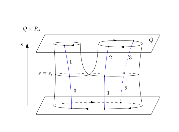
Figure 7. The image of $\bm{\Gamma}$ viewed as the graph in $Q\times\mathbb{R}_{s}$, where $\kappa=3$ and $\bm{s}_{\bm{t},\bm{\sigma},\bm{\rho}}$ with $\sigma_{i}=\begin{pmatrix}1&2&3\\ 1&3&2\end{pmatrix}$, $\sigma_{i+1}=\begin{pmatrix}1&2&3\\ 2&3&1\end{pmatrix}$, $\rho_{i+1}=\begin{pmatrix}1&2&3\\ 3&1&2\end{pmatrix}$ and $(a_{i}b_{i})=(12)$. The blue arcs labelled by $j=1,\ldots,\kappa$ denote the image of $\Gamma(s)_{j}(0)$. Each such $\Gamma(\cdot)_{j}(0)$ is allowed to have singularities at switching points.

Note that with $\bm{\Gamma}$ there is an associated sequence $\bm{t}$ of $t_{i}$’s corresponding to “moments of switching” as in (5).

Proposition 3.4.

For a generic choice of collections of pseudo-gradients $\bm{X}^{0},\ldots,\bm{X}^{\ell}$ and any $\bm{\gamma},\bm{\gamma}^{\prime}\in CM_{*}(\Lambda^{1}_{\kappa}(Q))$, the space $\widetilde{\mathcal{P}}(\bm{\gamma},\bm{\gamma}^{\prime};\bm{X}^{0},\ldots,\bm{X}^{\ell})$ is a smooth manifold of dimension $|\bm{\gamma}|-|\bm{\gamma}^{\prime}|-(n-2)\ell$. Furthermore, given some orientations of unstable manifolds of $\bm{\gamma}$ and $\bm{\gamma}^{\prime}$ there is a canonical orientation on $\widetilde{\mathcal{P}}(\bm{\gamma},\bm{\gamma}^{\prime};\bm{X}^{0},\ldots,\bm{X}^{\ell})$.

This proposition is a consequence of the discussion that follows. For $\{a,b\}\subset\{1,\ldots\kappa\}$ consider the subset $\Delta_{ab}\Omega^{1}_{\sigma}(Q)\subset\Omega^{1}_{\sigma}(Q)$ given by

(3.14) $$\Delta_{ab}\Omega^{1}_{\sigma}(Q)=\{\bm{\gamma}\in\Omega^{1}_{\sigma}(Q)\,|\,\text{ there exists }t\in(0,1)\text{ s.t. }\gamma_{a}(t)=\gamma_{b}(t)\}.$$

Let us consider the submersion

$$ev^{\kappa}_{[0,1]}\colon[0,1]\times\Omega^{1}_{\sigma}\to Q^{\kappa},$$

$$(t,\gamma_{1},\ldots,\gamma_{\kappa})\mapsto(\gamma_{1}(t),\ldots,\gamma_{\kappa}(t)).$$

Then $\Delta_{ab}\Omega^{1}_{\sigma}(Q)$ is obtained from the inverse image of

$$\Delta_{ab}Q^{\kappa}=\{(q_{1},\ldots,q_{\kappa})\in Q^{\kappa}\,|\,q_{a}=q_{b}\}\subset Q^{\kappa}$$

under $ev^{\kappa}_{[0,1]}$ by projecting to $\Omega^{1}_{\sigma}(Q)$. Therefore, $\Delta_{ab}\Omega^{1}_{\sigma}(Q)$ is a codimension $(n-1)$ submanifold of the Hilbert manifold $\Omega^{1}_{\sigma}(Q)$. Moreover, an orientation on $Q$ then induces an orientation on $\Delta_{ab}\Omega^{1}_{\sigma}(Q)$ (as it induces a coorientation on $\Delta_{ab}Q^{\kappa}$).

The diagonal $\Delta_{ab}\Omega^{1}_{\sigma}(Q)$ has an open subset $\Delta^{\text{sm}}_{ab}\Omega^{1}_{\sigma}(Q)\subset\Delta_{ab}\Omega^{1}_{\sigma}(Q)$ given by

(3.15) $$\Delta^{\text{sm}}_{ab}\Omega^{1}_{\sigma}(Q)=\{\bm{\gamma}\in\Omega^{1}_{\sigma}(Q)\,|\,\text{ there exists a unique }t\in(0,1)\text{ s.t. }\gamma_{a}(t)=\gamma_{b}(t)\}.$$

For $\bm{\gamma}\in\Delta^{\text{sm}}_{ab}\Omega^{1}_{\sigma}(Q)$ we denote by $t_{\Delta}(\bm{\gamma})$ the associated $t\in(0,1)$ for which $\gamma_{a}(t)=\gamma_{b}(t)$. The switching described in (5) of Definition 3.3 comes from the following smooth map

(3.16) $$sw_{ab}\colon\Delta^{\text{sm}}_{ab}\Omega^{1}_{\sigma}(Q)\to\Delta^{\text{sm}}_{ab}\Omega^{1}_{(\sigma(a)\sigma(b))\circ\sigma}(Q),$$

$$\bm{\gamma}\mapsto\bm{\gamma}^{\text{sw}}=(\gamma^{\text{sw}}_{1},\ldots,\gamma^{\text{sw}}_{\kappa}),\text{ where }$$

$$\gamma_{a}^{\text{sw}}(t)=\left\{\begin{array}[]{ll}\text{$\gamma_{a}(t)$ for $t\in[0,t_{\Delta}(\bm{\gamma})]$}\\ \text{$\gamma_{b}(t)$ for $t\in[t_{\Delta}(\bm{\gamma}),1]$}\end{array},\right.\quad\gamma_{b}^{\text{sw}}(t)=\left\{\begin{array}[]{ll}\text{$\gamma_{b}(t)$ for $t\in[0,t_{\Delta}(\bm{\gamma})]$}\\ \text{$\gamma_{a}(t)$ for $t\in[t_{\Delta}(\bm{\gamma}),1]$}\end{array},\right.$$

$$\gamma_{i}^{\text{sw}}=\gamma_{i},\text{ for }i\neq a,b.$$

We claim that $\text{sw}_{ab}$ is, moreover, a diffeomorphism. There is a conjugation action on $\Lambda^{1}_{\kappa}(Q)$ by any $\rho\in\mathfrak{S}_{\kappa}$ given by the following map

(3.17) $$\text{c}_{\rho}\colon\Lambda^{1}_{\kappa}(Q)\to\Lambda^{1}_{\kappa}(Q),$$

$$\bm{\gamma}\mapsto(\gamma_{\rho(1)},\ldots,\gamma_{\rho(\kappa)}).$$

Notice that

$$c_{\rho}\left(\Omega^{1}_{\sigma}(Q)\right)=\left(\Omega^{1}_{\rho\circ\sigma\circ\rho^{-1}}(Q)\right).$$

We now state, without proof, two general lemmas from the Morse theory on Hilbert manifolds. For more details we refer the reader to [AS10, Appendix A.2] and [AM06].

Lemma 3.5.

1. Let $\mathcal{M}$ be a Hilbert manifold with a pair $(X,f)$ that satisfies the conditions of Theorem 3.1. Let $x\in\text{crit}(f)$, $N$ be an $m$-dimensional submanifold of $\mathcal{M}$, and $\mathcal{M}_{0}$ be a codimension $m_{0}$ submanifold, such that both of them are disjoint from $\text{crit}(f)$. Then for a generic perturbation of $X$ supported away from the set of critical points the following sets

   (3.18) $$\mathcal{M}_{0}^{x}=W^{u}(x;X)\cap\mathcal{M}_{0},$$

   (3.19) $$\mathcal{M}_{0}^{N}=W^{u}(N;X)\cap\mathcal{M}_{0}$$

   are submanifolds of respective dimensions $\operatorname{ind}(x)-m_{0}$ and $(m+1)-m_{0}$.

2. Denote by $\widetilde{\mathcal{M}}_{0}^{x}$ and $\widetilde{\mathcal{M}}_{0}^{N}$ the stable manifolds of $\mathcal{M}_{0}^{x}$ and $\mathcal{M}_{0}^{N}$ under $X$, respectively. Then, if the submanifolds $W^{u}(x;X)$ and $N$ are oriented, and the submanifold $\mathcal{M}_{0}$ is cooriented, then the manifolds $\widetilde{\mathcal{M}}_{0}^{x}$ and $\widetilde{\mathcal{M}}_{0}^{N}$ carry canonical orientations. This can be expressed in terms of orientation lines (see Section 2.14) as

   (3.20) $$\zeta^{-1}\otimes|\eta_{\mathcal{M}_{0}}|\otimes|\widetilde{\mathcal{M}}_{0}^{x}|\cong|W^{u}(x)|,$$

   (3.21) $$\zeta^{-1}\otimes|\eta_{\mathcal{M}_{0}}|\otimes|\widetilde{\mathcal{M}}_{0}^{N}|\cong|W^{u}(N)|.$$

Lemma 3.6.

1. Let $\varphi\colon\mathcal{M}_{1}\to\mathcal{M}_{2}$ be a smooth map between Hilbert manifolds with $\mathcal{M}_{2}$ admitting a pair $(f_{2},X_{2})$ as in Theorem 3.1. Then for a given smooth $m$-dimensional submanifold $N$ of $\mathcal{M}_{1}$ and a critical point $y\in\mathcal{M}_{2}$ the set

   (3.22) $$N^{y}=N\cap\varphi^{-1}(W^{s}(y;X_{2}))$$

   is a submanifold of dimension $m-\operatorname{ind}(y)$ for generic perturbation of $X_{2}$ supported away from the critical points.

2. Denote by $\widetilde{N}$ and $\widetilde{N}^{y}$ the stable manifolds of $N$ and $N^{y}$, respectively. Then, if the manifold $W^{s}(y;X_{2})$ is cooriented and the manifold $N$ is oriented, the manifold $N^{y}$ carries canonical orientation. This can be expressed in terms of orientation lines as

   (3.23) $$|\eta_{W^{s}(y)}|\otimes|\widetilde{N}^{y}|\cong|\widetilde{N}|.$$

Remark 3.7.

There is a $(-1)^{\operatorname{ind}(y)}$ sign difference between the isomorphism in (3.23) and the one dictated by our convention for orienting a submanifold.

Proof of Proposition 3.4.

Let $\bm{\Gamma}=\left((\Gamma_{0},\ldots,\Gamma_{\ell}),\bm{s},\bm{\sigma},\bm{\rho}\right)\in\mathcal{P}(\bm{\gamma},\bm{\gamma}^{\prime};l)$ be a piecewise pseudo-gradient trajectory. Let us consider the following sequence of manifolds (see Figure 8 for an example with $\ell=2$):

$$W^{0}_{\bm{\sigma},\bm{\rho}}=W^{u}(\bm{\gamma};\bm{X}^{0})\cap\Delta^{\text{sm}}_{a_{0}b_{0}}\Omega^{1}_{\sigma_{0}}(Q),$$

$$W^{i+1}_{\bm{\sigma},\bm{\rho}}=W^{u}(c_{\rho_{i+1}}\circ sw_{a_{i}b_{i}}(W^{i}_{\bm{\sigma},\bm{\rho}});\bm{X}^{i+1})\cap\Delta^{\text{sm}}_{a_{i+1}b_{i+1}}\Omega^{1}_{\sigma_{i+1}}(Q)\text{ for }i=0,\ldots,\ell-2,$$

$$W^{\ell}_{\bm{\sigma},\bm{\rho}}=W^{\ell-1}_{\bm{\sigma},\bm{\rho}}\cap(c_{\rho_{\ell}}\circ sw_{a_{\ell-1}b_{\ell-1}})^{-1}\left(W^{s}(\bm{\gamma}^{\prime};\bm{X}^{\ell})\right).$$

Let us denote by $\widetilde{W}^{i}_{\bm{\sigma},\bm{\rho}}$ the manifold consisting of all points on piecewise pseudo-gradient trajectories connecting $\bm{\gamma}$ and $W^{i}_{\bm{\sigma},\bm{\rho}}$.

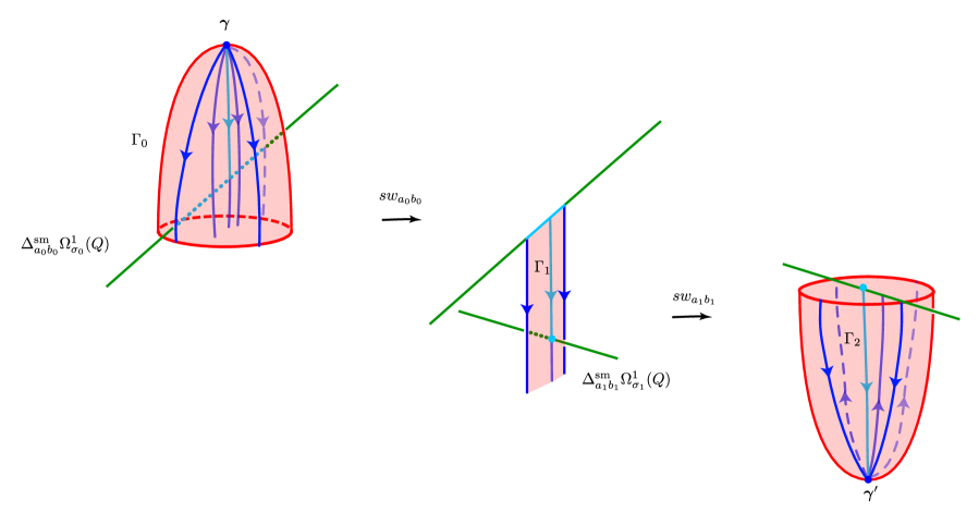
Figure 8. A cartoon depiction of $\mathcal{P}(\bm{\gamma},\bm{\gamma}^{\prime};2)$ with $n=3,|\bm{\gamma}|=3$ and $|\bm{\gamma}^{\prime}|=0$. A sample piecewise pseudo-gradient trajectory $\bm{\Gamma}=\leavevmode\nobreak\ (\Gamma_{0},\Gamma_{1},\Gamma_{2})\in\mathcal{P}(\bm{\gamma},\bm{\gamma}^{\prime};2)$ is depicted in turquoise. Portions of manifolds $W^{u}(\bm{\gamma};\bm{X}^{0}),W^{u}(c_{\rho_{1}}\circ sw_{a_{0}b_{0}}(W^{0}_{\bm{\sigma},\bm{\rho}});\bm{X}^{1})$ and $W^{s}(\bm{\gamma}^{\prime};\bm{X}^{2})$ are given in red. We also depict $W^{0}_{\bm{\sigma},\bm{\rho}}$ and $W^{1}_{\bm{\sigma},\bm{\rho}}$ in turquoise. The various diagonals in $\Lambda^{1}_{\kappa}(Q)$ are given in green.

Then from Lemma 3.5 it follows that $\widetilde{W}^{0},\ldots,\widetilde{W}^{\ell-1}$ are smooth manifolds and each $W^{i}$ has dimension

$$|\bm{\gamma}|-(n-2)(i+1).$$

Since each diagonal $\Delta^{\text{sm}}_{a_{i}b_{i}}\Omega^{1}_{\sigma_{0}}(Q)$ has a natural coorientation induced by the orientation of $Q$, by Lemma 3.5 there is a canonical orientation on each of $\widetilde{W}^{0},\ldots,\widetilde{W}^{\ell-1}$ given an orientation of $W^{u}(\bm{\gamma};\bm{X}^{0})$. More explicitly there are isomorphisms

(3.24) $$|\widetilde{W}^{0}|\cong\zeta^{2-n}\otimes o_{\bm{\gamma}},$$

(3.25) $$|\widetilde{W}^{i+1}|\cong\zeta^{2-n}\otimes|W^{i}|.$$

In the above, we use the isomorphism

(3.26) $$|\eta_{\Delta_{a_{i}b_{i}}^{\text{sm}}\Omega^{1}_{\sigma_{i+1}}(Q)}|\cong\zeta^{n-1},$$

given by the choice of orientation on $Q$.

By Lemma 3.6 the set $\widetilde{W}^{\ell}$ is then a smooth manifold of dimension

$$|\bm{\gamma}|-|\bm{\gamma}^{\prime}|-(n-2)\ell$$

with a canonical orientation induced by coorientation of $W^{s}(\bm{\gamma}^{\prime};\bm{X}^{\ell})$ and the orientation of $W^{\ell-1}$ as above, namely,

(3.27) $$o_{\bm{\gamma}^{\prime}}\otimes|\widetilde{W}^{\ell}|\cong|\widetilde{W}^{\ell-1}|.$$

We note that $\bm{\Gamma}\in\widetilde{W}^{\ell}$. Finally, we notice that $\widetilde{\mathcal{P}}(\bm{\gamma},\bm{\gamma}^{\prime};\ell)$ is a disjoint union of these $\widetilde{W}^{\ell}$ for all possible pairs $(\bm{\sigma},\bm{\rho})$. ∎

Note that there is an $\mathbb{R}$-action on $\widetilde{\mathcal{P}}(\bm{\gamma},\bm{\gamma}^{\prime};\ell)$ by the simultaneous shift of $(s_{1},\ldots,s_{l})$ and a simultaneous shift on all of the pseudo-gradient trajectories of a given piecewise pseudo-gradient trajectory. We denote the quotient by $\mathcal{P}(\bm{\gamma},\bm{\gamma}^{\prime};\ell)$. Given $\Gamma\in\widetilde{\mathcal{P}}(\bm{\gamma},\bm{\gamma}^{\prime};\ell)$, we denote its class in $\mathcal{P}(\bm{\gamma},\bm{\gamma}^{\prime};\ell)$ by $[\Gamma]$.

We are now ready to define the Morse free multiloop complex. For a critical multiloop $\bm{\gamma}\in\mathcal{P}^{\bm{L}}_{\kappa}$ we associate rank-$1$ abelian group $o_{\bm{\gamma}}$ generated by orientations of $W^{u}(\bm{\gamma};\bm{X})$ and we set as before

(3.28) $$o_{\bm{\gamma}}^{\mathbb{Q}}=\mathbb{Q}\otimes_{\mathbb{Z}}o_{\bm{\gamma}}.$$

Then we set

(3.29) $$V^{\kappa}=\bigoplus_{\bm{\gamma}\in\mathcal{P}_{\kappa}^{\bm{L}}}o_{\bm{\gamma}}^{\mathbb{Q}},$$

and

(3.30) $$V^{\kappa}_{i}=\bigoplus_{|\bm{\gamma}|=i}o_{\bm{\gamma}}^{\mathbb{Q}}.$$

Definition 3.8.

The Morse chain free multiloop complex $CM_{*}\left(\Lambda^{1}_{\kappa}(Q)\right)$ is a graded vector subspace of $W_{\kappa}\llbracket\hbar\rrbracket$ given by

(3.31) $$CM_{m}\left(\Lambda^{1}_{\kappa}(Q)\right)=\sum_{i+(n-2)j=m}V_{i}^{\kappa}\hbar^{j}=\sum_{i+(n-2)j=m}V_{i}^{\kappa}[(2-n)j].$$

By composing isomorphisms in equations (3.24), (3.25), (3.27) and permuting the terms (respecting the Koszul sign rule; see Section 2.14) we get a canonical isomorphism

(3.32) $$\big{|}\widetilde{\mathcal{P}}(\bm{\gamma},\bm{\gamma}^{\prime};\ell)\big{|}^{-1}\otimes o_{\bm{\gamma}}\cong o_{\bm{\gamma}^{\prime}}\otimes\zeta^{(n-2)\ell}\cong o_{\bm{\gamma}^{\prime}}\bigl{[}(2-n)\ell\bigr{]}.$$

When $|\bm{\gamma}|-|\bm{\gamma}^{\prime}|-(n-2)\ell=1$, given a piecewise pseudo-gradient trajectory $[\bm{\Gamma}]\leavevmode\nobreak\ \in\leavevmode\nobreak\ \mathcal{P}(\bm{\gamma},\bm{\gamma}^{\prime};\ell)$, the above isomorphism can be rewritten as

(3.33) $$|\mathbb{R}\partial_{s}|^{-1}\otimes o_{\bm{\gamma}}\cong o_{\bm{\gamma}^{\prime}}\bigl{[}(2-n)\ell\bigr{]}.$$

Fixing the upward orientation (arising from the positive gradient direction), which corresponds to the opposite orientation on $\mathbb{R}$, induces a morphism

(3.34) $$\partial_{[\bm{\Gamma}]}\colon o_{\bm{\gamma}}^{\mathbb{Q}}\to o_{\bm{\gamma}^{\prime}}^{\mathbb{Q}}\bigl{[}(2-n)\ell\bigr{]}.$$

We extend this map to any generator $[\bm{\gamma}]\hbar^{j}$ of $CM_{*}\bigl{(}\Lambda^{1}_{\kappa}(Q)\bigr{)}$ by tensoring the above isomorphism with $\zeta^{(n-2)j}$ on the right:

(3.35) $$\partial_{[\bm{\Gamma}]}\colon o_{\bm{x}}\otimes\zeta^{(n-2)j}\to\otimes o_{\bm{x}^{\prime}}\bigl{[}(2-n)\ell\bigr{]}\otimes\zeta^{(n-2)j}\cong o_{\bm{x}^{\prime}}\bigl{[}(2-n)(\ell+j)\bigr{]}.$$

We may now define the differential on Morse free multiloop complex $CM_{*}\bigl{(}\Lambda^{1}_{\kappa}(Q)\bigr{)}$ by

(3.36) $$\partial\colon CM_{*}(\Lambda^{1}_{\kappa}(Q))\to CM_{*-1}(\Lambda^{1}_{\kappa}(Q)),$$

$$\partial([\bm{\gamma}]\hbar^{j})=\sum_{\begin{subarray}{c}\ell\geq 0,|\bm{\gamma}^{\prime}|=|\bm{\gamma}|-(n-2)\ell-1,\\ [\bm{\Gamma}]\in\mathcal{P}(\bm{\gamma},\bm{\gamma}^{\prime};\ell)\end{subarray}}\partial_{[\bm{\Gamma}]}([\bm{\gamma}]\hbar^{j}).$$

where $[\bm{\gamma}]\hbar^{j}$ is some generator of $o_{\bm{\gamma}}^{\mathbb{Q}}[(2-n)j]$ for $j\geq 0$. We devote the following section to showing that this is indeed a chain complex.

For the later use we define the reflected cochain complex $CM^{*}_{-}(\Lambda^{1}_{\kappa}(Q))$ as follows. First, set

$$V_{\kappa,-}^{i}=\bigoplus_{|\bm{\gamma}|=-i}(o_{\bm{\gamma}}^{-1})^{\mathbb{Q}}.$$

Then

$$CM^{m}_{-}(\Lambda^{1}_{\kappa}(Q))=\sum_{-(i+(n-2)j)=m}V^{i}_{\kappa,-}[(n-2)j].$$

Applying our conventions (2.136) we notice that

$$o_{\bm{\gamma}}^{-1}[(n-2)j]\cong\zeta^{(2-n)j}\otimes o_{\bm{\gamma}}^{-1}\cong(o_{\bm{\gamma}}[(2-n)j])^{-1}.$$

Then clearly the isomorphism (3.33) also induces a morphism

(3.37) $$d_{[\bm{\Gamma}]}\colon(o_{\bm{\gamma}}^{-1})^{\mathbb{Q}}\to o_{\bm{\gamma}}^{-1}[(n-2)j]^{\mathbb{Q}}.$$

The differential on the reflected Morse miltiloop complex is then given by

(3.38) $$\partial\colon CM^{*}_{-}(\Lambda^{1}_{\kappa}(Q))\to CM^{*+1}_{-}(\Lambda^{1}_{\kappa}(Q)),$$

$$d([\bm{\gamma}_{-}]\hbar^{-j})=\sum_{\begin{subarray}{c}\ell\geq 0,|\bm{\gamma}^{\prime}|=|\bm{\gamma}|-(n-2)\ell-1,\\ [\bm{\Gamma}]\in\mathcal{P}(\bm{\gamma},\bm{\gamma}^{\prime};\ell)\end{subarray}}d_{[\bm{\Gamma}]}([\bm{\gamma}]\hbar^{-j}).$$

At last, we claim that there is a natural reflection chain map between the two complexes, inducing a homology isomorphism

(3.39) $$\mathcal{I}\colon CM_{-}^{*}\bigl{(}\Lambda^{1}_{\kappa}(Q)\bigr{)}\to CM_{-*}\bigl{(}\Lambda^{1}_{\kappa}(Q)\bigr{)},$$

which one obtains by applying the isomorphism $\ell\cong\ell^{-1}$ for orientation lines and inspecting Koszul sign rule, see Section 2.14.

3.3. Compactness

Since a piecewise gradient trajectory is not action-decreasing, the nonemptiness of $\mathcal{P}(\bm{\gamma},\bm{\gamma}^{\prime};\ell)$ does not imply $\mathcal{A}_{\bm{L}}(\bm{\gamma})\geq\mathcal{A}_{\bm{L}}(\bm{\gamma}^{\prime})$. However, we can still show that $\mathcal{A}_{\bm{L}}(\bm{\gamma}^{\prime})-\mathcal{A}_{\bm{L}}(\bm{\gamma})$ is $C^{0}$-bounded, so for each $\ell\geq 0$, $\mathcal{P}(\bm{\gamma},\bm{\gamma}^{\prime};\ell)$ is empty for all but finitely many $\bm{\gamma}^{\prime}$. Therefore, the chain complex $CM^{*}_{\kappa}(\Lambda Q)$ is locally finite.

Lemma 3.9.

Fix a generic choice of a collection of pseudo-gradient vector field tuples $\bm{X}^{0},\ldots,\bm{X}^{\ell}$, given $|\bm{\gamma}|-|\bm{\gamma}^{\prime}|-(n-2)\ell\leq 2$, the space $\mathcal{P}(\bm{\gamma},\bm{\gamma}^{\prime};\ell)$ admits a compactification.

Sketch of the proof.

Given $(2-n)l+|\bm{\gamma}^{\prime}|-|\bm{\gamma}|\leq 2$, $\mathcal{P}(\bm{\gamma},\bm{\gamma}^{\prime};l)$ is a smooth manifold of dimension $\leq 1$ by Lemma 3.4. We need to consider all possible limiting behaviors of a sequence of elements in $\mathcal{P}_{*}(\bm{\gamma},\bm{\gamma}^{\prime};l)$. The proof is similar to [HKTY, Lemma A.9]. We sketch the cases similar to [HKTY, Lemma A.9] and emphasize the difference.

Let

$$[\Gamma^{r}]=[((\Gamma^{r}_{0},\ldots,\Gamma^{r}_{l}),(\bm{s}^{r},\bm{\sigma}^{r},\bm{\rho}^{r})]$$

be a sequence of piecewise gradient trajectories in $\mathcal{P}(\bm{\gamma},\bm{\gamma}^{\prime};l)$ parametrized by $r\in\mathbb{N}$. We can assume that the premutation data $((\sigma_{1}^{r},\ldots,\sigma_{\ell}^{r}),(\rho^{r}_{1},\ldots,\rho^{r}_{\ell}))=(\bm{\sigma},\bm{\rho})$ is constant for this sequence. As $r\to\infty$, if $[\Gamma^{r}]$ does not limit to an interior element of $\mathcal{P}_{*}(\bm{\gamma},\bm{\gamma}^{\prime};l)$, then there are four possibilities:

(1) $s^{r}_{i}-s^{r}_{i+1}\to+\infty$ for some $1\leq i\leq l-1$. This corresponds to breaking along $\Gamma^{r}_{i}$. Breaking along $\Gamma^{r}_{0}$ or $\Gamma^{r}_{l}$ is similar. In the limit $r\to\infty$, $\Gamma_{r}$ degenerates to a broken piecewise pseudo-gradient trajectory which lies in $\mathcal{P}(\bm{\gamma},\bm{\gamma}^{\prime\prime};\ell_{1})\times\mathcal{P}(\bm{\gamma}^{\prime\prime},\bm{\gamma}^{\prime};\ell_{2})$, where $\ell_{1}+\ell_{2}=\ell$. The sum of the expected dimensions of $\mathcal{P}_{*}(\bm{\gamma},\bm{\gamma}^{\prime\prime};\ell_{1})$ and $\mathcal{P}(\bm{\gamma}^{\prime\prime},\bm{\gamma}^{\prime};\ell_{2})$ is equal to $|\bm{\gamma}|-|\bm{\gamma}^{\prime}|-(n-2)\ell-2$. Therefore, if $|\bm{\gamma}|-|\bm{\gamma}^{\prime}|-(n-2)\ell\leq 1$, $s^{r}_{i}-s^{r}_{i+1}\to+\infty$ does not occur for a generic choice of pseudo-gradient vector fields. If $|\bm{\gamma}|-|\bm{\gamma}^{\prime}|-(n-2)\ell=2$, this is the required degeneration for the differential on $CM^{*}_{\kappa}(\Lambda_{\kappa}^{1}Q)$ to be well-defined.

(2) $s^{r}_{i}-s^{r}_{i+1}\to 0$ for some $1\leq i\leq\ell-1$. In the limit $r\to\infty$, two switchings occur at the same $s$. This case is discussed in [HKTY, Lemma A.9]. We refer the reader to Figure 9 for an illustration.

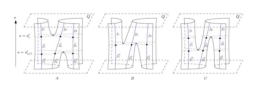
Figure 9. The image of $\sqcup_{i,s}\Gamma_{i}(s)$ viewed as the graph in $Q\times\mathbb{R}_{s}$. The blue arc labelled by $j$ denotes the image of $\Gamma_{i}(s)_{j}(0)$. As $r\to\infty$, $s^{r}_{i}-s^{r}_{i+1}\to 0$ as shown by (A); the limit is shown by (B), where two switchings occur simultaneously; the family (A) is paired up with another family (C). Note that the allowance of all permutation sequences in Definition 3.3 is necessary for the existence of (C).

(3) Generically, a 1-parameter family of piecewise pseudo-gradient trajectories may undergo a birth-death bifurcation. This is also discussed in [HKTY, Lemma A.9] and we omit the proof here.

(4) $t_{i+1}^{r}\to 0$ for some $i=0,\ldots,\ell-1$. Let us assume that $t_{i}\to 0^{+}$, meaning that all these times are in $[0,\epsilon)$ for $i\gg 0$ and a small $\epsilon>0$. For the limit of the paths $\Gamma^{r}_{i}(s_{i+1})_{a_{i}}$ and $\Gamma^{r}_{i}(s_{i+1})_{b_{i}}$ we have that $\Gamma^{\infty}_{i}(s_{i+1})_{a_{i}}$ and $\Gamma^{\infty}_{i}(s_{i+1})_{b_{i}}$ intersect at $t_{i+1}^{\infty}=0$.

We consider a subset of the closure $\overline{\Delta}_{ab}\Omega^{1}_{\sigma}(Q)\subset\Omega^{1}_{\sigma}(Q)$ given by

(3.40) $$\Delta^{\text{sm},0,1}_{ab}\Omega^{1}_{\sigma}(Q)=\{\bm{\gamma}\in\Omega^{1}_{\sigma}(Q)\,|\,\text{ there exists a unique }t\in[0,1]\text{ s.t. }\gamma_{a}(t)=\gamma_{b}(t)\}$$

which can be also given as a disjoint union

$$\Delta^{\text{sm},0,1}_{ab}\Omega^{1}_{\sigma}(Q)=\Delta^{\text{sm}}_{ab}\Omega^{1}_{\sigma}(Q)\sqcup\Delta^{\text{sm},0}_{ab}\Omega^{1}_{\sigma}(Q)\sqcup\Delta^{\text{sm},1}_{ab}\Omega^{1}_{\sigma}(Q)\text{, where }$$

$$\Delta^{\text{sm},0}_{ab}\Omega^{1}_{\sigma}(Q)=\{\bm{\gamma}\in\Delta^{\text{sm},0,1}_{ab}\Omega^{1}_{\sigma}(Q)\,|\,\gamma_{a}(0)=\gamma_{b}(0)\},$$

$$\Delta^{\text{sm},1}_{ab}\Omega^{1}_{\sigma}(Q)=\{\bm{\gamma}\in\Delta^{\text{sm},0,1}_{ab}\Omega^{1}_{\sigma}(Q)\,|\,\gamma_{a}(1)=\gamma_{b}(1)\}.$$

Notice that both $\Delta^{0}_{ab}\Omega^{1}_{\sigma}(Q)$ and $\Delta^{1}_{ab}\Omega^{1}_{\sigma}(Q)$ are codimension $n$ submanifolds. Additionally, we point out that

(3.41) $$\Delta^{\text{sm},0}_{ab}\Omega^{1}_{\sigma}(Q)=\Delta^{\text{sm},1}_{\sigma^{-1}(a)\sigma^{-1}(b)}\Omega^{1}_{\sigma}(Q).$$

With these notations we then have $\Gamma_{i}^{\infty}(s_{i+1})\in\Delta^{0}_{a_{i}b_{i}}\Omega^{1}_{\sigma_{i}}(Q)$. Using notations from the proof of Proposition 3.4 we consider the following set

$$W^{i}_{\bm{\sigma},\bm{\rho},i_{0,1}}=W^{u}(c_{\rho_{i}}\circ sw_{a_{i-1}b_{i-1}}(W^{i-1}_{\bm{\sigma},\bm{\rho}});\bm{X}^{i})\cap\Delta^{\text{sm},0,1}_{a_{i}b_{i}}\Omega^{1}_{\sigma_{i}}(Q).$$

Replacing $W^{i}_{\bm{\sigma},\bm{\rho}}$ with this set we then obtain $W^{\ell}_{\bm{\sigma},\bm{\rho},i_{0,1}}$ following the procedure in the proof of Proposition 3.4. Note that $\bm{\Gamma}^{\infty}$ corresponds to a point of $W^{\ell}_{\bm{\sigma},\bm{\rho},i_{0}}\subset W^{\ell}_{\bm{\sigma},\bm{\rho},i_{0,1}}$. Consider a new collection $\bm{\rho}^{\prime}$ with $\rho^{\prime}_{j}=\rho_{j}$ for $j\neq i+1$ and $\rho^{\prime}_{i+1}$ satisfying:

(3.42) $$\rho^{\prime}_{i+1}(a_{i})=\rho_{i+1}(b_{i}),\,\rho^{\prime}_{i+1}(b_{i})=\rho_{i+1}(a_{i}),\,\rho^{\prime}_{i+1}(c)=\rho_{i+1}(c)\text{ for }c\neq a_{i},b_{i}.$$

Expediting (3.13) and (3.42) one can see that

$$(\rho^{\prime-1}_{i+1}\circ\sigma_{i+1}\circ\rho^{\prime}_{i+1})\circ\sigma_{i}^{-1}=(a_{i}b_{i}).$$

Hence, $W^{\ell}_{\bm{\sigma},\bm{\rho}^{\prime}}$ and $W^{\ell}_{\bm{\sigma},\bm{\rho}^{\prime},i_{0,1}}$ are well-defined. Now applying (3.41) we have

$$\bm{\Gamma}^{\infty}\in W^{\ell}_{\bm{\sigma},\bm{\rho}^{\prime},i_{1}}\subset W^{\ell}_{\bm{\sigma},\bm{\rho}^{\prime},i_{0,1}}.$$

Finally, since $W^{\ell}_{\bm{\sigma},\bm{\rho}^{\prime},i_{0,1}}$ is of dimension $1$ as $W^{\ell}_{\bm{\sigma},\bm{\rho},i_{0,1}}$ for generic choice of pseudo-gradient vector fields $\bm{X}^{i}$’s, there must be a $1$-dimensional family of pseudo-gradient trajectories in $W^{\ell}_{\bm{\sigma},\bm{\rho}^{\prime}}$ limiting to $\bm{\Gamma}^{\infty}$ (see Figure 10 for an example of such a family near $s_{i+1}$). Therefore, we may represent $\bm{\Gamma}^{\infty}$ as a limit of a sequence $\bm{\Gamma}^{-r}\in W^{\ell}_{\bm{\sigma},\bm{\rho}^{\prime}}.$ The constructed above sequence corresponds to $t_{i+1}^{-r}\to 1$ which implies that such singular behaviors are paired up and do not constitute part of the boundary of $\mathcal{P}(\bm{\gamma},\bm{\gamma}^{\prime};\ell)$.

We notice that the choice of $\bm{\rho}^{\prime}$ in the argument above is the main reason why in Definition 3.3 we have introduced permutation data $\bm{\rho}$.

Figure 10. On the left side trajectory $[\Gamma^{r}]$ is depicted near $s_{i+1}$. On the right side, we depict trajectory $[\Gamma^{-r}]$ that is constructed in the proof.

Finally, we note that the compactification of $\mathcal{P}(\bm{\gamma},\bm{\gamma}^{\prime};\ell)$ exists since $\bm{\gamma}$ is of finite Morse index. ∎

As an immediate corollary of Lemma 3.9 we obtain

Proposition 3.10.

$\partial^{2}=0$.

Proof.

By Lemma 3.9, $\#\mathcal{P}(\bm{\gamma},\bm{\gamma}^{\prime};\ell)$ is finite whenever $|\bm{\gamma}^{\prime}|=|\bm{\gamma}|-(n-2)\ell-1$. We also point out that for a given $\gamma$ the space $\#\mathcal{P}(\bm{\gamma},\bm{\gamma}^{\prime};\ell)$ is empty for all but finitely many $\bm{\gamma}^{\prime}$ by the Palais-Smale condition 24. Given $|\bm{\gamma}|-|\bm{\gamma}^{\prime}|-(n-2)\ell=2$, applying the continuation procedure described in Lemma 3.9 the boundary of the compactification of $\mathcal{P}(\bm{\gamma},\bm{\gamma}^{\prime};l)$ may be regarded as a finite number of broken pseudo-gradient trajectories, i.e.,

$$\partial\overline{\mathcal{P}}(\bm{\gamma},\bm{\gamma}^{\prime};\ell)=\bigsqcup_{\begin{subarray}{c}\ell_{1}+\ell_{2}=\ell,\\ |\bm{\gamma}|-|\bm{\gamma}^{\prime\prime}|=|\bm{\gamma}^{\prime\prime}|-|\bm{\gamma}^{\prime}|=(n-2)\ell+1\end{subarray}}\mathcal{P}(\bm{\gamma},\bm{\gamma}^{\prime\prime};\ell_{1})\times\mathcal{P}(\bm{\gamma}^{\prime\prime},\bm{\gamma}^{\prime};\ell_{2}).$$

To finish the proof it is enough to compare the composition map $\partial_{[\bm{\Gamma}_{2}]}\circ\partial_{[\bm{\Gamma}_{1}]}$ and the map induced by boundary orientation. That is,

(3.43) $$|\mathbb{R}\partial_{s}|^{-1}\otimes\big{|}\mathcal{P}(\bm{\gamma},\bm{\gamma}^{\prime};\ell)\big{|}^{-1}\otimes o_{\bm{\gamma}}\cong o_{\bm{\gamma}^{\prime}}\bigl{[}(2-n)\ell\bigr{]},$$

(3.44) $$|\mathbb{R}\partial_{s}\bm{\Gamma}_{2}|^{-1}\otimes|\mathbb{R}\partial_{s}\bm{\Gamma}_{1}|^{-1}\otimes o_{\bm{\gamma}}\cong|\mathbb{R}\partial_{s}\bm{\Gamma}_{2}|^{-1}\otimes o_{\bm{\gamma}^{\prime\prime}}\bigl{[}(2-n)\ell_{1}\bigr{]}\cong o_{\bm{\gamma}^{\prime}}\bigl{[}(2-n)\ell\bigr{]}.$$

Now it remains to notice that $\partial_{s}\bm{\Gamma}_{1}$ with the preferred orientation as in (3.33) is an outward pointing vector. Therefore, $\partial|_{o_{\bm{\gamma}}}^{2}=0$. We leave it to the reader to verify that $\partial|_{o_{\bm{\gamma}}[(2-n)j]}^{2}=0$ for any $j>0$. ∎

We write $CM_{*}(\Lambda^{1}_{\kappa}(Q);\bm{L},\bm{X})$ and $HM_{*}(\Lambda^{1}_{\kappa}(Q);\bm{L},\bm{X})$ to indicate the specific choice of $\bm{L}=\{L_{1},\ldots,L_{\kappa}\}$ and pseudo-gradient vector fields $\bm{X}$.

Proposition 3.11.

The homology groups $HM_{*}(\Lambda^{1}_{\kappa}(Q);\bm{L},\bm{X})$ do not depend on the choice of $\bm{L}=\{L_{1},\ldots,L_{\kappa}\}$ and pseudo-gradient vector fields $\bm{X}$.

Proof.

According to [AS10] changing $\bm{L}$ or pseudo-gradient fields $\bm{X}$ induces chain homotopy at the level of standard Morse chain complexes. Hence, if we were considering only pseudo-gradient trajectories with $\ell=0$ the statement would immediately follow. We then claim that showing that changing one of $L_{i}$’s or $\bm{X}_{j}$’s alone induces a chain homotopy in the presence of switchings is similar to the above-mentioned line of the argument. ∎

4. The isomorphism between the Heegaard Floer symplectic cohomology and the homology of the free multiloop complex

In this section, we define a chain map from the Floer complex to the Morse complex

$$\mathcal{F}\colon SC^{*}_{\kappa,\text{unsym}}(T^{*}Q)\to CM_{\kappa n-*}^{\kappa}(\Lambda Q),$$

by counting rigid elements in a mixed moduli space which combines holomorphic curves and piecewise gradient trajectories. We establish an analogue of the Viterbo isomorphism theorem in the context of Heegaard Floer symplectic cohomology by showing that $\mathcal{F}$ is a quasi-isomorphism.

In this section, we assume that $Q$ is an orientable closed manifold with vanishing second Stiefel-Whitney class

$$w_{2}(TQ)\leavevmode\nobreak\ \in\leavevmode\nobreak\ H^{2}(T^{*}Q;\mathbb{Z}/2).$$

This allows one to fix a spin structure on $Q$ regarded as a Lagrangian submanifold in $T^{*}Q$. We also note that the approach in this section is parallel to [HKTY, Section 3].

We point out that we work here with the unsymmetrized version of HFSH introduced in Section 2.13 and sometimes we abuse notations and do not specify that we work in this context as it is understood throughout this section.

4.1. The half-cylinder Hurwitz space

We start by introducing the space of branched covers of a half-cylinder in the context of Section 2.13.

Definition 4.1.

Let $\sigma,\sigma_{0}\in\mathfrak{S}_{\kappa}$. For given $\chi>0$ define $\mathcal{H}^{\sigma,\sigma_{0},\geq 0}_{\kappa,\chi}$ to be the set of tuples

$$\left(\pi\colon S\to\mathbb{R}_{\geq 0}\times S^{1},\bm{p}^{+},\bm{a}^{+},\bm{P}^{0},\bm{a}^{0},B\right)\text{, where}$$

1. $S$ is a Riemann surface of Euler characteristic $\chi$ with positive punctures $\bm{p}^{+}=\{p^{+}_{1},\ldots,p^{+}_{l(\bm{\mu})}\}$ and boundary components $\bm{P}^{0}=\{P^{0}_{1},\ldots,P^{0}_{\ell(\sigma_{0})}\}$. Denote by $\overline{S}$ the compactification of $S$ such that $S=\overline{S}\setminus\bm{p}^{+}$.

2. $\bm{a}^{+}=(a_{1}^{+},\ldots,a_{\kappa}^{+})$ is a collection of positive asymptotic markers at positive punctures $p_{i}^{+}$ such that for each $p_{i}^{+}$ there are exactly $\mu_{i}(\sigma)$ asymptotic markers $a_{i_{1}}^{+},\ldots,a_{i_{\mu_{i}}}^{+}\in\mathcal{S}^{1}_{p_{i}^{+}}S=(T_{p_{i}^{+}}S\setminus\{0\})/\mathbb{R}_{>0}$, and these are exactly the indices permuted by $c_{i}(\sigma)$ abd they appear on $\mathcal{S}^{1}_{p_{i}^{+}}$ in the order prescribed by the cycle $c_{i}(\sigma)$.

   Analogously we choose marked points, which we simply call markers, on $\bm{P}^{0}$ such that for each boundary component $P^{0}_{i}$ there are exactly $\mu_{i}(\sigma_{0})$ markers.The permutation on the set of markers induced by walking along $P_{i}^{0}$ in the boundary orientation direction is required to be equal to $c_{i}(\sigma_{0})$.

3. $\pi\colon S\longrightarrow\mathbb{R}_{\geq 0}\times S^{1}$ is a holomorphic branched cover with simple branched points away from $+\infty$ and boundary $\partial S=\bm{P}^{0}$. At $+\infty$ the branching profile is given by $\bm{\mu}$ and for each boundary component $P^{0}_{i}$ the restriction $\pi|_{P^{0}_{i}}$ is the $\mu_{i}^{0}$-cover of $\{0\}\times S^{1}$.

4. The map induced by $\pi$ from $\mathcal{S}^{1}_{p_{i}^{+}}S$ to $\mathcal{S}^{1}_{+\infty}(\mathbb{R}_{\geq 0}\times S^{1})$ sends all asymptotic markers assigned to $p_{i}^{+}$ to the asymptotic marker $1\in\mathcal{S}^{1}_{+\infty}(\mathbb{R}_{\geq 0}\times S^{1})$. The markers $a_{i}^{0}$’s are all sent to $(0,0)\in R_{\geq 0}\times S^{1}$ under $\pi$.

5. $B=(q_{1},\ldots q_{b})$, is an ordered collection of points in $\mathbb{R}_{>0}\times S^{1}$ of simple branching, where $b=-\chi$.

Figure 11. The tuple $((s,\pi),\bm{s}_{\bm{t},\bm{\sigma},\bm{\rho}})$ above is an element of $\mathcal{T}^{\sigma,\sigma_{0},\sigma^{\prime}}_{-3,\ell}$ for $\kappa=4$ with $\sigma=(1342)$, $\sigma_{0}=(14)(23)$, and we do not specify $\sigma^{\prime}$.

Following the approach of Section 2.5 we define a portion $\widehat{\mathcal{H}}^{\sigma,\sigma_{0},\geq 0}_{\kappa,\chi}$ of the compactification $\overline{\mathcal{H}}^{\sigma,\sigma_{0},\geq 0}_{\kappa,\chi}$ (which we will not specify here). Namely, an element of $\widehat{\mathcal{H}}^{\sigma,\sigma_{0},\geq 0}_{\kappa,\chi}$ may have several levels of covers of the cylinder $\mathbb{R}\times S^{1}$ above the cover of half cylinder. That is

Definition 4.2.

The space of smooth half-cylindrical buildings $\widehat{\mathcal{H}}^{\sigma,\sigma_{0},\geq 0}_{\kappa,\chi}$ consists of

$$[(\overrightarrow{C}=(C_{0},\ldots,C_{n}),S=S_{0}\cup\ldots\cup S_{n},(\bm{v}^{n-1},\ldots,\bm{v}^{0}),(\bm{m}^{n-1},\ldots,\bm{m}^{0}),\pi]$$

where

1. $\pi|_{S_{0}}\colon S_{0}\to\mathbb{R}_{\geq 0}\times S^{1}$ is a branched cover of a half cylinder with data of markers on the boundary, but without asymptotic markers. In other words, it comes from an element of ${\mathcal{H}^{\sigma^{\prime},\sigma_{0},\geq 0}_{\kappa,\chi_{2}}}$ for some $\sigma^{\prime}\in\mathfrak{S}_{\kappa}$ by forgetting asymptotic markers;

2. $\bm{m}^{0}$ is a tuple of matching markers corresponding to the nodes $\bm{v}^{0}$ connecting $S_{0}$ and $S_{1}$ (see (4) of Definition 2.5 for more details);

3. $[(\overrightarrow{C}_{>0}=(C_{n},\ldots,C_{1}),S_{>0}=S_{n}\cup\ldots\cup S_{1},(\bm{v}^{n-1},\ldots,\bm{v}^{1}),(\bm{m}^{n-1},\ldots,\bm{m}^{1}).\pi|_{S_{>0}}]$ comes from an element of $\widehat{\mathcal{H}}^{\sigma,\sigma^{\prime}}_{\kappa,\chi_{1}}$ with forgotten asymptotic markers at negative punctures of $C_{1}$ (see Definition 2.5).

4. It holds that $\chi_{1}+\chi_{2}=\chi$.

Similarly to $\widehat{\mathcal{H}}^{\bm{\mu},\bm{\mu}^{\prime}}_{\kappa,\chi}$ (see Definition 2.20) a codimension $1$ boundary of $\widehat{\mathcal{H}}^{\sigma,\sigma_{0},\geq 0}_{\kappa,\chi}$ can be given as the images under natural embeddings of spaces

(4.1) $$\bigsqcup_{\begin{subarray}{c}\chi_{1}+\chi_{2}=\chi,\\ \sigma^{\prime}\in\mathfrak{S}_{\kappa}\end{subarray}}\mathcal{H}^{\sigma,\sigma^{\prime}}_{\kappa,\chi_{1}}\times_{\bm{m}}\mathcal{H}^{\sigma^{\prime},\sigma_{0},\geq 0}_{\kappa,\chi_{2}}.$$

4.2. Floer data for the half-cylinder Hurwitz space

We set up the perturbation data on the half-cylinder Hurwitz space following Section 2.8. First, we note that there is a wnbc groupoid $\widehat{\mathscr{H}}^{\sigma,\sigma_{0},\geq 0}_{\kappa,\chi}$ built via construction similar to the one given in Section 2.6.

As in the Section 2.8 there is a smooth choice of positive cylindrical ends $\{\delta^{i}_{+}\}_{i=1}^{i=\ell(\bm{\sigma})}$ and finite cylinders $\delta^{j}_{i,r}$ over the whole $\widehat{\mathscr{H}}^{\sigma,\sigma_{0},\geq 0}_{\kappa,\chi}$.

A Floer datum on $(S,\pi)\in(\widehat{\mathscr{H}}^{\sigma,\sigma_{0},\geq 0}_{\kappa,\chi})^{\vee}_{H}$ (here $(S,\pi)$ is assumed to be away from the boundary) is a collection $(H_{(S,\pi)},F_{(S,\pi)},J_{(S,\pi)})$, where

1. $H_{(S,\pi)}\colon S\to\mathcal{H}(\hat{M})$ is a domain-dependent Hamiltonian function, required to coincide with $H_{0}$ on cylindrical ends and finite cylinders and is equal to $0$ near the boundary $\partial S$;

2. a domain-dependent function $F_{(S,\pi)}\in C^{\infty}(\hat{M})$ on $S$ such that conditions given in 2 are satisfied (we note that on a cylinder with assigned cycle $c\in\mathfrak{S}_{\kappa}$ the function $F$ has to coincide with $F_{c}$ away from the collars) and additionally $F$ vanishes near $\partial S$;

3. a domain-dependent almost complex structure $J_{(S,\pi)}\colon S\to\mathcal{J}_{\hat{M}}$ coinciding with $J_{t}$ as in (2.21) at each cylindrical end and at each finite cylinder

As in the case of Hurwitz spaces, there exists a choice of consistent Floer data $(H,F,J)$ on $\widehat{\mathscr{H}}^{\sigma,\sigma_{0},\geq 0}_{\kappa,\chi}$ in the sense of Section 2.8. As before we will use the notation $H^{\text{tot}}=H+F$.

4.3. The mixed moduli space

Consider $\bm{x}\in\mathcal{P}_{\text{unsym}}(T^{*}Q)$, $\bm{\gamma}\in\mathcal{P}_{\kappa}^{\bm{L}}$ and a permutation $\sigma_{0}\in\mathfrak{S}_{\kappa}$. We set $\sigma=\sigma(\bm{x})$ and $\sigma^{\prime}=\sigma(\bm{\gamma})$.

We define the mixed moduli space $\mathcal{T}^{\sigma_{0}}_{\chi,\ell}(H^{\text{tot}},J,\bm{X};\bm{x},\bm{\gamma})$ to be the space of tuples

(4.2) $$\left((S,\pi\colon S\to\mathbb{R}_{\geq 0}\times S^{1}),u=(\pi,v),\bm{\Psi}\right),$$

where $(S,\pi)\in\mathcal{H}^{\sigma,\sigma_{0},\geq 0}_{\kappa,\chi}$, and $u$ is a map

$$u\colon S\to\mathbb{R}_{\geq 0}\times S^{1}\times T^{*}Q,$$

and $\bm{\Psi}=((\Psi_{0},\ldots,\Psi_{\ell}),\bm{s},\bm{\sigma},\bm{\rho})$ is a collection of maps

$$\Psi_{i}\colon[s_{i+1},s_{i}]\to\Omega^{1}_{\sigma_{i}}(Q),$$

where $\bm{s}=(s_{0},\ldots,s_{\ell+1})$ with $s_{0}=0$, $s_{\ell+1}=-\infty$ and $0>s_{1}>\ldots>s_{\ell}>-\infty$, $\bm{\sigma}$ and $\bm{\rho}$ are two collections of permutations in $\mathfrak{S}_{\kappa}$ with a leading term of $\bm{\sigma}$ being exactly the $\sigma_{0}$ as above (here we allow ourselves slight abuses of notation).

The map $u=(\pi,v)$ satisfies

(4.3) $$\begin{dcases}(dv-Y_{(S,\pi)})^{0,1}=0,\text{ with respect to }J_{(S,\pi)};\\ \lim_{s\to+\infty}v\circ\delta_{i}^{+}(s,\cdot)=x^{c_{i}(\sigma)}(\cdot)\text{ for }i=1,\ldots,\ell(\sigma);\\ \operatorname{Im}(v|_{\partial S})\subset Q.\end{dcases}$$

Here $Y_{(S,\pi)}$ is $1$-form associated $H^{\text{tot}}_{(S,\pi)}$ as in (2.73). We point out that as in Lemma 2.31 the map $u$ can be regarded as a pseudo-holomorphic map with respect to the almost complex structure $\underline{J}^{H^{\text{tot}}}_{(S,\pi)}$ defined as in Section 2.8.

Let us denote the space of pairs $\left((S,\pi),u\right)$ satisfying (4.3) by $\mathcal{H}^{\sigma,\sigma_{0},\geq 0}_{\kappa,\chi}(H^{\text{tot}},J;\bm{x})$. Then there is a natural evaluation map

(4.4) $$\mathcal{EV}\colon\mathcal{H}^{\sigma,\sigma_{0},\geq 0}_{\kappa,\chi}(H^{\text{tot}},J;\bm{x})\to\Omega^{1}_{\sigma_{0}}(Q)$$

given by sending a pair $\left((S,\pi),u\right)$ to the restriction of $u$ to $\partial S$.

We then require for collection $\Psi$ to satisfy the following:

1. $\Psi_{0}(0)=\mathcal{EV}(u)$, $\Psi_{l}(-\infty)=\bm{\gamma}$.

2. $\Psi_{i}^{\prime}(s)=\bm{X}^{i}(\Psi_{i}(s))$.

3. For each $i$ such that $0\leq i\leq\ell-1$ there is a transposition $(a_{i}b_{i})\in\mathfrak{S}_{\kappa}$ such that

   $$(\rho^{-1}_{i+1}\circ\sigma_{i+1}\circ\rho_{i+1})\circ\sigma_{i}^{-1}=(\sigma_{i}(a_{i})\sigma_{i}(b_{i})).$$

4. For $a_{i},b_{i}\in\{1,\ldots,\kappa\}$ satisfying the above for $i=0,\ldots,\ell-1$ there exists $t_{i}\in(0,1)$, so that

   $$\Psi_{i+1}(s_{i+1})_{\rho_{i+1}(a_{i})}(t)=\left\{\begin{array}[]{ll}\text{$\Psi_{i}(s_{i+1})_{a_{i}}(t)$ for $t\in[0,t_{i+1}]$}\\ \text{$\Psi_{i}(s_{i+1})_{b_{i}}(t)$ for $t\in[t_{i+1},1]$}\end{array},\right.$$

   $$\Psi_{i+1}(s_{i+1})_{\rho_{i+1}(b_{i})}(t)=\left\{\begin{array}[]{ll}\text{$\Psi_{i}(s_{i+1})_{b_{i}}(t)$ for $t\in[0,t_{i+1}]$}\\ \text{$\Psi_{i}(s_{i+1})_{a_{i}}(t)$ for $t\in[t_{i+1},1]$}\end{array}.\right.$$

5. $\Psi_{i+1}(s_{i+1})_{\rho_{i+1}(j)}=\Psi_{i+1}(s_{i+1})_{j}$ for $j\neq a_{i},b_{i}$.

Lemma 4.3.

For a tuple of Hamiltonian orbits $\bm{x}\in\mathcal{P}_{unsym}(T^{*}Q)$, a multiloop $\bm{\gamma}\in\mathcal{P}_{\kappa}^{\bm{L}}$, and a generic choice of Floer data on $\mathcal{H}^{\sigma,\sigma_{0},\geq 0}_{\kappa,\chi}$, and a generic collection $\bm{X}$ of pseudo-gradient vector fields $\bm{X}$, the space $\mathcal{T}^{\sigma_{0}}_{\chi,\ell}(H^{\text{tot}},J,\bm{X};\bm{x},\bm{\gamma})$ is a smooth manifold of dimension

$$\kappa n-|\bm{x}|-|\bm{\gamma}|-(n-2)(\ell-\chi).$$

Moreover, given an orientation of $Q$ and a spin structure on the pull-back of tangent bundle $TQ$ to $T^{*}Q$ there is an induced orientation $\mathcal{T}^{\sigma_{0}}_{\chi,\ell}(H^{\text{tot}},J,\bm{X};\bm{x},\bm{\gamma})$.

Proof.

First, we show that $\mathcal{H}^{\sigma,\sigma_{0},\geq 0}_{\kappa,\chi}(H^{\text{tot}},J;\bm{x})$ is a smooth manifold along the lines of the argument in Theorem 2.33 (compare with [Abo11, Section 3] for the $\kappa=1$ case). For index calculation, we glue the operator $D_{u}$ associated with a given element of $\mathcal{H}^{\sigma,\sigma_{0},\geq 0}_{\kappa,\chi}(H^{\text{tot}},J;\bm{x})$ to the operator $D_{\bm{x}}$ associated with a tuple of Hamiltonian orbits $\bm{x}$, obtained by the direct product of operators $D_{x^{c_{i}(\sigma)}}$ (see (2.118)) to obtain an operator $D_{u}\#D_{\bm{x}}$ from a surface with no punctures. Then

$$\operatorname{ind}(D_{u}\#D_{\bm{x}})=n(\chi+\ell(x))$$

by [Sei08a, Proposition 11.13] and

$$\operatorname{ind}(D_{\bm{x}})=n(\ell(\bm{x})-\kappa)-|\bm{x}|.$$

Hence

$$\operatorname{ind}(D_{u})=\kappa n-|\bm{x}|+n\chi$$

and then one concludes as in Lemma 2.35 that the dimension of $\mathcal{H}^{\sigma,\sigma_{0},\geq 0}_{\kappa,\chi}(H^{\text{tot}},J;\bm{x})$ is equal to

(4.5) $$\kappa n-|\bm{x}|+(n-2)\chi.$$

Given a spin structure on $TQ$ regarded as a subbundle of $TT^{*}Q$, following [Sei08a, Proposition 11.13] and [Abo11, Appendix A], there are isomorphisms

(4.6) $$\big{|}\mathcal{H}^{\sigma,\sigma_{0},\geq 0}_{\kappa,\chi}(H^{\text{tot}},J;\bm{x})\big{|}\cong o_{\bm{x}}^{-1}\otimes\big{|}\mathcal{H}^{\sigma,\sigma_{0},\geq 0}_{\kappa,\chi}\big{|}\otimes|Q|^{\ell(\sigma_{0})}\otimes\zeta^{\kappa n+n(\chi-\ell(\sigma_{0})}\cong\zeta^{(n-2)\chi}\otimes o_{\bm{x}}^{-1}\otimes\zeta^{\kappa n}.$$

For the later isomorphism, we use the fixed orientation on $Q$ to get trivialization $|Q|\cong\zeta^{n}$ and the standard orientation on $\mathcal{H}^{\sigma,\sigma_{0},\geq 0}_{\kappa,\chi}$ to get $|\mathcal{H}^{\sigma,\sigma_{0},\geq 0}_{\kappa,\chi}|\cong\zeta^{-2\chi}$; we note that in the second isomorphism, there is a Koszul sign involved that we do not mention explicitly.

Next, we claim that for generic Floer data, the image of the space $\mathcal{H}^{\sigma,\sigma_{0},\geq 0}_{\kappa,\chi}(H^{\text{tot}},J;\bm{x})$ under the evaluation map $\mathcal{EV}$ is a smooth submanifold of $\Omega^{1}_{\sigma_{0}}(Q)$. It is implied by [AS06, Theorem 3.8] and more generally by the discussion in [AS10, Section 5]. Finally, one may conclude the proof by applying the argument of Proposition 3.4 to show that for a generic choice of pseudo-gradient vector fields $\bm{X}^{i}$ the piecewise pseudo-gradient trajectories connecting the image of $\mathcal{H}^{\sigma,\sigma_{0},\geq 0}_{\kappa,\chi}(H^{\text{tot}},J;\bm{x})$ under $\mathcal{EV}$ with $\bm{\gamma}$ constitute a smooth manifold.

As for the orientation on $\mathcal{T}^{\sigma_{0}}_{\chi,\ell}(H^{\text{tot}},J,\bm{X};\bm{x},\bm{\gamma})$, one may argue as in the proof of Proposition 3.4 that

(4.7) $$o_{\bm{\gamma}}\otimes\big{|}\mathcal{T}^{\sigma_{0}}_{\chi,\ell}(H^{\text{tot}},J,\bm{X};\bm{x},\bm{\gamma})\big{|}\cong\zeta^{(2-n)\ell}\otimes\big{|}\mathcal{H}^{\sigma,\sigma_{0},\geq 0}_{\kappa,\chi}(H^{\text{tot}},J;\bm{x})\big{|}.$$

By combining (4.6) and (4.7) one gets an orientation on $\mathcal{T}^{\sigma_{0}}_{\chi,\ell}(H^{\text{tot}},J,\bm{X};\bm{x},\bm{\gamma})$ induced by a choice of a generator of $o_{\bm{x}}$. ∎

Lemma 4.4.

For a generic choice of Floer data on $\mathcal{H}^{\sigma,\sigma_{0},\geq 0}_{\kappa,\chi}$, and a collection $\bm{X}$ of pseudo-gradient vector fields, and an arbitrary tuple of Hamiltonian orbits $\bm{x}\in\mathcal{P}_{\text{unsym}}(T^{*}Q)$ and $m\geq 0$, the space

$$\underset{\ell-\chi=m,\,\sigma_{0}\in\mathfrak{S}_{\kappa}}{\bigsqcup}\mathcal{T}^{\sigma_{0}}_{\chi,\ell}(H^{\text{tot}},J,\bm{X};\bm{x},\bm{\gamma})$$

is empty for all but finitely many $\bm{\gamma}\in\mathcal{P}_{\kappa}^{\bm{L}}$.

Proof.

We omit the proof as it follows from the Palais-Smale condition 24, see [AS06] for details. ∎

From now on we will omit the auxiliary data in the notation for the mixed moduli spaces.

Asside on Kuranishi replacements. As in Section 2.9, for $n\geq 3$ a sequence of elements in the mixed moduli space may converge to an pair with Floer side admitting ghost bubbles. More precisely, a sequence of curves $(u_{i},\Psi_{(i)})$, $i=1,2,\dots$, in $\mathcal{T}^{\sigma_{0}}_{\chi,\ell}(H^{\text{tot}},J,\bm{X};\bm{x},\bm{\gamma})$, after passing to a subsequence, can limit to

$$(u_{\infty}=u_{\infty,1}\cup u_{\infty,2},\Psi_{(\infty)}),$$

where:

• the main part $u_{\infty,1}$ is the union of components that are not ghost bubbles; each component of the $u_{\infty,1}$ is somewhere injective; and

• $u_{\infty,2}$ is a union of ghost bubbles, i.e., locally constant maps where the domain is a possibly disconnected compact Riemann surface (possibly with boundary) and $u_{\infty,2}$ maps to points on $\operatorname{Im}(u_{\infty,1})$.

To remedy this we introduce we introduce Kuranishi replacements $\mathcal{T}^{\sigma_{0},\sharp}_{\chi,\ell}(H^{\text{tot}},J,\bm{X};\bm{x},\bm{\gamma})$ satisfying similar requirements to 1-3 (see [HKTY, Section 3.2.2] for more specifics). As before, we will pass to Kuranishi replacements whenever neccessary and drop $\sharp$ from the notation.

Before diving into the discussion of the compactification of mixed moduli spaces of dimension $1$ we introduce two new types of boundary behavior. Let us fix tuples $\bm{x}\in\mathcal{P}_{\text{unsym}}(T^{*}Q)$ and $\bm{\gamma}\in\mathcal{P}^{\bm{L}}_{\kappa}$ satisfying for some $\chi\leq 0,\ell\geq 0$:

$$\kappa n-|\bm{x}|-1=|\bm{\gamma}|+(n-2)(\ell-\chi).$$

Definition 4.5.

The Type I singular mixed moduli space $\mathcal{T}^{\sigma_{0},\mathrm{I}}_{\chi,\ell}(\bm{x},\bm{\gamma})$ is a space of tuples

$$\left((S,\pi),u,\bm{\Psi}\right)$$

as in (4.2) with the following differences:

1. $(S,\pi)$ represents a point in $\overline{\mathcal{H}}^{\sigma,\sigma_{0},\geq 0}_{\kappa,\chi}$, such that (only) one of the branch points in $B$ has $s$-coordinate equal to $0$;

2. $\bm{\Psi}=\left((\Psi_{1},\ldots,\Psi_{\ell}),\bm{s}=(s_{0},s_{1},\ldots,s_{\ell+2}),\bm{\sigma}=(\sigma_{1},\ldots,\sigma_{\ell}),\bm{\rho}=(\rho_{2},\ldots,\rho_{\ell+1})\right)$ is a tuple (note the different number of elements in each tuple) with conditions that $s_{0}=s_{1}$ and $\sigma_{1}=\sigma_{0}$.

(a)

Figure 12. Approaching a Type I singularity.

Remark 4.6.

Heuristically, a Type I boundary singularity is a result of a ramification point approaching the boundary and adding a new switching point on the Morse side at $s=0$ (see Figure 12). The number of switching points of the curves in $\mathcal{T}^{\sigma_{0},\mathrm{I}}_{\chi,\ell}(\bm{x},\bm{\gamma})$ is equal to $\ell+1$. We point out here that $s_{1}$ is not a genuine switching point since there is no naturally assigned permutation $\rho_{1}$ with it and the pseudo-gradient flows from $s_{1}=s_{0}$ to $s_{2}$ are prescribed by the old $\sigma_{0}$.

Definition 4.7.

The Type II singular mixed moduli space $\mathcal{T}^{\sigma_{0},\mathrm{II}}_{\chi,\ell}(\bm{x},\bm{\gamma})$ is the space of tuples

$$\left((S,\pi),u,\bm{\Psi}\right)$$

as in (4.2) with the following differences:

1. $(S,\pi\colon S\to\mathbb{R}_{\geq 0}\times S^{1})$ is a branched cover with a set of branched points consisting of $|B|=-\chi+1$ points with (only) one of these points having $s$-coordinate equal to $0$;

2. $\bm{\Psi}=\left((\Psi_{1},\ldots,\Psi_{\ell}),\bm{s}=(s_{0},s_{1},\ldots,s_{\ell+1}),\bm{\sigma}=(\sigma_{0},\sigma_{1},\ldots,\sigma_{\ell}),\bm{\rho}=(\rho_{1},\ldots,\rho_{\ell})\right)$ is a tuple with conditions that $s_{0}=s_{1}$, and for markers $a^{0}_{a_{0}}$, $a^{0}_{b_{0}}$ such that positive arcs connecting these markers to the next (in counterclockwise order) markers on $\partial S$ contain the ramification point it holds that

   $$(\rho^{-1}_{1}\circ\sigma_{1}\circ\rho_{1})\circ\sigma_{0}^{-1}=(\sigma_{0}(a_{0})\sigma_{0}(b_{0})).$$

(a)

Figure 13. Approaching a Type II singularity.

Remark 4.8.

A Type II boundary singularity is a result of $s_{1}$ approaching $s_{0}$ accompanied by the creation of a new ramification point on $S$ (as well as a branch point on the target; see Figure 13 for a schematic picture). The Euler characteristic of curves in $\mathcal{T}^{\sigma_{0},\mathrm{II}}_{\chi,\ell}(\bm{x},\bm{\gamma})$ is equal to $\chi-1$.

Remark 4.9.

Following discussion of Remarks 4.6 and 4.8, we note that given a curve in $\mathcal{T}^{\sigma_{0},\mathrm{I}}_{\chi,\ell}(\bm{x},\bm{\gamma})$ we may obtain a curve in $\mathcal{T}^{\sigma_{0}^{\prime},\mathrm{II}}_{\chi+1,\ell+1}(\bm{x},\bm{\gamma})$ by arbitrary adding $\sigma_{0}^{\prime}$ and $\rho_{1}$ to the data in Definition 4.5 satisfying condition (2) in Definition 4.7. Hence one geometrical curve of $\mathcal{T}^{\sigma_{0},\mathrm{I}}_{\chi,\ell}(\bm{x},\bm{\gamma})$ corresponds to $\kappa!$ curves of

$$\bigsqcup_{\sigma_{0}^{\prime}\in\mathfrak{S_{\kappa}}}\mathcal{T}^{\sigma_{0}^{\prime},\mathrm{II}}_{\chi+1,\ell+1}(\bm{x},\bm{\gamma}).$$

This phenomenon is crucial for the map defined via counting mixed curves to be a chain map.

Lemma 4.10.

For a generic choice of consistent Floer data on $\widehat{\mathscr{H}}^{\sigma,\sigma_{0},\geq 0}_{\kappa,\chi}$ and a collection of pseudo-gradient vector fields $\bm{X}$, a tuple of Hamiltonian orbits $\bm{x}\in\mathcal{P}_{\text{unsym}}(T^{*}Q)$ and a multiloop $\bm{\gamma}\in\mathcal{P}_{\kappa}^{\bm{L}}$ satisfying

(4.8) $$\kappa n-|\bm{x}|-|\bm{\gamma}|-(n-2)(\ell-\chi)=1,$$

the wnb groupoid $\mathscr{T}^{\sigma_{0}}_{\chi,\ell}(H^{\text{tot}},J,\bm{X};\bm{x},\bm{\gamma})(U)$ admits a compactification $\overline{\mathscr{T}}^{\sigma_{0}}_{\chi,\ell}(H^{\text{tot}},J,\bm{X};\bm{x},\bm{\gamma})$.

Sketch of the proof.

As in the proof of 2.38 one may show that there is a portion of the boundary corresponding to the vertical stretching, and we leave it to the reader to fill in the details. Points of this type on the boundary of $\overline{\mathscr{T}}^{\sigma_{0}}_{\chi,\ell}(H^{\text{tot}},J,\bm{X};\bm{x},\bm{\gamma})$ correspond to elements of

(4.9) $$\bigsqcup_{\begin{subarray}{c}\bm{x}^{\prime}\in SC^{*}_{\kappa}(T^{*}Q),\\ \chi_{1}+\chi_{2}=\chi\end{subarray}}\mathscr{M}^{\chi_{1},\text{ind}=1}(\bm{x},\bm{x}^{\prime})\times\mathcal{T}^{\sigma_{0},\text{ind}=0}_{\chi_{2},\ell}(\bm{x}^{\prime},\bm{\gamma})$$

counted with weights $\frac{1}{\kappa!}$.

The second type of boundary degeneration corresponds to stretching on the Morse side and is treated in Lemma 3.9. These points of the boundary are elements of

(4.10) $$\bigsqcup_{\begin{subarray}{c}\bm{\gamma}^{\prime}\in CM_{\kappa n-*}(\Lambda^{1}_{\kappa}(Q)),\\ \ell_{1}+\ell_{2}=\ell\end{subarray}}\mathcal{T}^{\sigma_{0},\text{ind}=0}_{\chi,\ell_{1}}(\bm{x},\bm{\gamma}^{\prime})\times\mathcal{P}^{\text{ind}=1}(\bm{\gamma}^{\prime},\bm{\gamma};\ell_{2}).$$

One last case that we have to analyze is the boundary nodal degeneration with a possible occurrence of almost ghost bubbles attached along the boundary. Let us first treat this scenario. Namely, assume that $(u_{i},\Psi_{i})$ limits to $(u_{\infty}=u_{\infty,1}\cup u_{\infty,2},\Psi_{\infty})$, where $u_{\infty,2}$ is null-homologous (see 2) has domain attached to the domain of $u_{\infty,1}$ along $k$ boundary nodes. We then have

$$\operatorname{ind}u_{\infty}=\operatorname{ind}u_{i}+k(n-2)$$

by (4.5). On the other hand, the appearance of a boundary node along the Lagrangian $\{0\}\times S^{1}\times Q$ is a codimension $(n+1)-2\cdot 1=n-1$ condition since the Lagrangian is $(n+1)$-dimensional and the boundary of the domain is mapped to a real $1$-dimensional curve. In total, we get a dimension drop of

$$k(n-1)-k(n-2)=k.$$

Hence, $u_{\infty,2}$ can be attached only along the boundary node $1$ and it must have only $1$ boundary component. This component can not be a disk, since there have to be at least two ramification points on it. Therefore, $\operatorname{ind}(u_{\infty,2})<0$ and it violates 3 and 2.

Finally, from the above analysis, it follows that there could be no more than $1$ boundary node. If no ghost bubbles appear, this leaves us with the two singular types of boundary points $\mathcal{T}^{\sigma_{0},\mathrm{I}}_{\chi,\ell}(\bm{x},\bm{\gamma})$ and $\mathcal{T}^{\sigma_{0},\mathrm{II}}_{\chi,\ell}(\bm{x},\bm{\gamma})$. ∎

4.4. Chain map

To define a morphism $\mathcal{F}$

(4.11) $$\mathcal{F}\colon SC^{*}_{\kappa,\text{unsym}}(T^{*}Q)\to CM_{\kappa n-*}\bigl{(}\Lambda^{1}_{\kappa}(Q)\bigr{)},\\$$

we first consider the canonical isomorphism

(4.12) $$o_{\bm{\gamma}}[(2-n)(\ell-\chi)]\otimes o_{\bm{x}}\cong\big{|}\mathcal{T}^{\sigma_{0}}_{\chi,\ell}(\bm{x},\bm{\gamma})\big{|}^{-1}\otimes\zeta^{\kappa n}.$$

When the dimension of the mixed moduli space is $0$ the above provides the isomorphism

(4.13) $$o_{\bm{x}}\cong\bigl{(}o_{\bm{\gamma}}[(2-n)(\ell-\chi)]\bigr{)}^{-1}\otimes\zeta^{\kappa n},$$

which induces a morphism

(4.14) $$f_{[u,\bm{\Psi}]}\colon o_{\bm{x}}\rightarrow\bigl{(}o_{\bm{\gamma}}[(2-n)(\ell-\chi)]\bigr{)}^{-1}[-\kappa n].$$

We extend it to $o_{\bm{x}}[(n-2)j]$ for $j>0$ by simply multiplying the above with $\zeta^{(2-n)j}$ on the left. We first define $\mathcal{F}^{-}\colon SC^{*}_{\kappa}(T^{*}Q)\to CM_{-}^{*}\bigl{(}\Lambda^{1}_{\kappa}(Q)\bigr{)}[-\kappa n]$ as above to be

(4.15) $$\mathcal{F}^{-}([\bm{x}]\hbar^{j})=\sum_{\begin{subarray}{c}|\bm{\gamma}|=\kappa n-|\bm{x}|-(n-2)(\ell-\chi),\\ \ell\geq 0,\chi\leq 0,\,\sigma_{0}\in\mathfrak{S}_{\kappa},\\ (u,\bm{\Psi})\in\mathcal{T}^{\sigma_{0}}_{\chi,\ell}(\bm{x},\bm{\gamma})\end{subarray}}(-1)^{|\bm{x}|+(n-2)j}\cdot\frac{f_{(u,\bm{\Psi})}([x]\hbar^{j})}{(\kappa!)^{\ell}}.$$

The morphism $\mathcal{F}$ is then obtained by composing $\mathcal{F}^{-}$ with a $\kappa n$-shift of $CM_{-}^{*-\kappa n}\bigl{(}\Lambda^{1}_{\kappa}(Q)\bigr{)}[-\kappa n]$ and the reflection chain map $\mathcal{I}\colon CM_{-}^{*}\bigl{(}\Lambda^{1}_{\kappa}(Q)\bigr{)}\to CM_{-*}\bigl{(}\Lambda^{1}_{\kappa}(Q)\bigr{)}$; see (3.39).

By Lemma 4.10, $\mathcal{T}^{\sigma_{0}}_{\chi,\ell}(\bm{x},\bm{\gamma})$ is finite, hence the maps $\mathcal{F}^{-}$ and $\mathcal{F}$ are well-defined.

Theorem 4.11.

The map $\mathcal{F}^{-}$ is a chain map.

Proof.

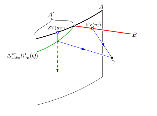
Figure 14. The neighborhood of a nodal degeneration. Each point on the thick lines $A$ and $B$ denotes the 1-dimensional family of image of the evaluation map $\mathcal{EV}(u)$ for some $u$ defined above. The intersection of $A$ and $B$ represents $\mathcal{EV}(u_{*})$ where $u_{*}$ is a nodal curve. The blue arcs denote pseudo-gradient trajectories. The green arc denotes $\Delta^{\text{sm}}_{a_{0}b_{0}}\Omega^{1}_{\sigma_{0}}(Q)$. The entire quadrilateral denotes the image of the gradient trajectories starting from $A$.

We analyze the codimension 1 boundary of $\mathcal{T}^{\sigma_{0}}_{\chi,\ell}(\bm{x},\bm{\gamma})$. A special codimension 1 phenomenon is the nodal degeneration along the zero section $Q$ which corresponds to a point $\left((S,\pi_{*}),u_{*},\bm{\Psi}_{*}\right)$ of the Type II singular space $\mathcal{T}^{\sigma_{0},\mathrm{II}}_{\chi+1,\ell+1}(\bm{x},\bm{\gamma})$. This point can also be regarded (by dropping $\sigma_{0}$ and $\rho_{1}$ from the $\bm{\Psi}$ data) as a point of the Type I singular mixed moduli space $\mathcal{T}^{\sigma_{1},\mathrm{I}}_{\chi,\ell}(\bm{x},\bm{\gamma})$. Here $\sigma_{1}$ is a permutation from $\bm{\sigma}$-data of $\bm{\Psi}_{*}$. We give a sketch of the proof that there is a $1$-dimensional family of points in $\mathcal{T}^{\sigma_{1}}_{\chi,\ell}(\bm{x},\bm{\gamma})$ converging to such a point.

For $\left((S,\pi_{*}),u_{*},\bm{\Psi}\right)$ as above, we assume that the multiloop $\mathcal{EV}\left(u_{*}\right)\in\Omega^{1}_{\sigma_{0}}(Q)$ is sufficiently generic. Let $R\left(\mathcal{EV}\left(u_{*}\right)\right)\in\Omega^{1}_{\sigma_{1}}(Q)$ be the switching of the multiloop $\mathcal{EV}\left(u_{*}\right)$. Refer to Figure 3.2, which gives a schematic description of a neighborhood of $\mathcal{EV}\left(u_{*}\right)\in\Lambda^{1}_{\kappa}(Q)$; in the figure $\mathcal{EV}\left(u_{*}\right)$ is identified with $R\left(\mathcal{EV}\left(u_{*}\right)\right)$.

Let

1. $B$ be the set of $\mathcal{EV}\left(u_{\mathrm{I}}\right),u_{\mathrm{I}}\in\mathcal{H}^{\sigma,\sigma_{1},\geq 0}_{\kappa,\chi}(\bm{x})$, such that there is a piecewise smooth pseudo-gradient trajectory $\bm{\Psi}$ from $\mathcal{EV}\left(u_{\mathrm{I}}\right)$ to $\bm{\gamma}$;

2. $A$ be the set of $\mathcal{EV}\left(u_{\mathrm{II}}\right),u_{\mathrm{II}}\in\mathcal{H}^{\sigma,\sigma_{0},\geq 0}_{\kappa,\chi+1}(\bm{x})$; and

3. $A^{\prime}\subset A$ be the subset consisting of $\mathcal{EV}\left(u_{\mathrm{II}}\right),u_{\mathrm{II}}\in\mathcal{H}^{\sigma,\sigma_{0},\geq 0}_{\kappa,\chi+1}(\bm{x})$, for which there is a piecewise smooth pseudo-gradient trajectory $\bm{\Psi}$ from $\mathcal{EV}\left(u_{\mathrm{II}}\right)$ to $\bm{\gamma}$.

We have $u_{*}\in\mathcal{H}^{\sigma,\sigma_{0},\geq 0}_{\kappa,\chi+1}(\bm{x}),\mathcal{EV}\left(u_{*}\right)\in A$, and $R\left(\mathcal{EV}\left(u_{*}\right)\right)\in\partial B$.

Step 1 (Description of $\mathcal{H}^{\sigma,\sigma_{0},\geq 0}_{\kappa,\chi+1}$ and $\mathcal{H}^{\sigma,\sigma_{1},\geq 0}_{\kappa,\chi}(\bm{x})$ near $u_{*}$) If $\operatorname{dim}\mathcal{H}^{\sigma,\sigma_{1},\geq 0}_{\kappa,\chi}(\bm{x})=b+1$, then

$$\operatorname{dim}\mathcal{H}^{\sigma,\sigma_{0},\geq 0}_{\kappa,\chi+1}(\bm{x})=b+1+(n-2),$$

by (4.5).

The following theorem generalizes the gluing result of Ekholm and Shende [ES19, Section 4.4.4]. Let $U\left(u_{*}\right)$ be a neighborhood of $u_{*}$ in $\mathcal{H}^{\sigma,\sigma_{0},\geq 0}_{\kappa,\chi+1}(\bm{x})$ and let

$$Z=\{u_{\mathrm{II}}\in\mathcal{H}^{\sigma,\sigma_{0},\geq 0}_{\kappa,\chi+1}(\bm{x})\mid u_{\mathrm{II}}\text{ has a node along }s=0\}.$$

Theorem 4.12.

There exists a neighborhood of $Z\cap U(u_{*})$ in $\mathcal{H}^{\sigma,\sigma_{0},\geq 0}_{\kappa,\chi+1}(\bm{x})$ of the form $D^{b}\times D^{n-1}$, such that $Z\cap U(u_{*})=D^{b}\times\{0\}$. Moreover, $Z\cap U(u_{*})$ can be viewed as an open subset of $\partial\overline{\mathcal{H}}^{\sigma,\sigma_{1},\geq 0}_{\kappa,\chi}(\bm{x})$.

Sketch of proof of Theorem 4.12.

We convert the desired perturbations of a nodal curve into a smooth one into a commonly used SFT-type gluing result (see, for example, [FOOO] which treats holomorphic curves before/after Lagrangian surgery). “Zooming in” near the intersection point, we consider the following local model:

1. the ambient symplectic/almost complex manifold is $\mathbb{C}^{n}$ with the standard symplectic form,

2. the Lagrangian boundary condition is the standard $\mathbb{R}^{n}\subset\mathbb{C}^{n}$, and

3. the punctures of the finite energy holomorphic curves under consideration limit to chords (in a Morse-Bott family) from $S^{n-1}$ to itself, where $S^{n-1}\subset S^{2n-1}$ is the Legendrian boundary at infinity of $\mathbb{R}^{n}$.

We consider pairs of half-planes of the form

$$\begin{gathered}P_{1}\left(z_{3},\ldots,z_{n-1}\right)\coloneqq\left\{\left(z_{1},\ldots,z_{n-1}\right)\in\mathbb{C}^{n-1}\mid z_{2}=z_{1},z_{1}\in\mathbb{H},z_{3},\ldots,z_{n-1}\in\mathbb{R}\right\},\\ P_{2}\coloneqq\left\{\left(z_{1},\ldots,z_{n-1}\right)\in\mathbb{C}^{n-1}\mid z_{2}=-z_{1},z_{1}\in\mathbb{H},z_{3}=\cdots=z_{n-1}=0\right\}.\end{gathered}$$

For the pair $P_{1}(0,\ldots,0)$ and $P_{2}$ we consider gluing along the node using model

$$C_{c}\coloneqq\left\{\left(z_{1},z_{2},z_{3},\ldots,z_{n-1}\right)\in\mathbb{C}^{n-1}\mid z_{1}\in\mathbb{H},z_{2}^{2}-z_{1}^{2}=c,\,z_{3}=\ldots=z_{n-1}=0\right\}_{c\in\mathbb{R}_{\geq 0}}.$$

Writing

$$i_{\dot{F}_{z_{3},\ldots,z_{n-1};c}}\colon\dot{F}_{z_{3},\ldots,z_{n-1};c}\to\mathbb{C}^{n-1}$$

for the holomorphic embedding with image $(P_{1}(z_{3},\ldots,z_{n-1}),P_{2})$ whenever one of $z_{i}$’s is not equal to $0$ and with the image $C_{c}$ otherwise. We also take a double cover

$$\pi_{z_{3},\ldots,z_{n-1};c}\colon\dot{F}_{z_{3},\ldots,z_{n-1};c}\rightarrow\mathbb{C}$$

with image $\mathbb{H}$. The map

$$\left(i_{\dot{F}_{z_{3},\ldots,z_{n-1};c}},\pi_{z_{3},\ldots,z_{n-1};c}\right)\colon\dot{F}_{z_{3},\ldots,z_{n-1};c}\rightarrow\mathbb{C}^{n-1}\times\mathbb{C}$$

is the holomorphic map to $\mathbb{C}^{n}$ with boundary on $\mathbb{R}^{n}$.

Half-planes are Morse-Bott regular, since they can be doubled into standard complex lines in $\mathbb{C}^{n-1}$ and a curve is regular if and only if its double is; the same also holds for $C_{c}$. Finally, we leave it to the reader to verify the necessary SFT-type gluing result for finite energy holomorphic curves with Lagrangian boundary in this Morse-Bott case. ∎

Step 2 (Descriptions of $A$ and $B$) Now suppose that having a gradient trajectory that goes to $\bm{\gamma}$ is a codimension $b$ condition for some $b\geq 0$. Recalling the definitions of $A$ and $B$ from earlier in the proof, $\operatorname{dim}B=1$. Theorem 4.12 and the genericity of the evaluation map $\mathcal{EV}$ give:

Claim 4.13.

There exists an identification $A\cap\mathcal{EV}\left(U\left(u_{*}\right)\right)\simeq D^{b}\times D^{n-1}$ with respect to which $\mathcal{EV}\left(u_{*}\right)=(0,0),\,\mathcal{EV}\left(Z\cap U\left(u_{*}\right)\right)=D^{b}\times\{0\}$, and $R\left(\mathcal{EV}\left(u_{*}\right)\right)$ is the unique point on $\partial B$ on a neighborhood of $R\left(\mathcal{EV}\left(u_{*}\right)\right)$.

Step 3 (Description of $A^{\prime}$)

Claim 4.14.

Under the identification from Claim 3.5, $A^{\prime}\cap\mathcal{EV}\left(U\left(u_{*}\right)\right)=\{0\}\times r$, where $r$ is a radial ray in $D^{n-1}$ emanating from $0$.

Proof of Claim 4.14.

By transversality for mixed moduli, we know that $A^{\prime}$ is a $1$-dimensional manifold (see Lemma 4.3). By definition, for any point of $A^{\prime}$ finite time flow of $\bm{X}^{0}$ hits a point of $\Delta^{\text{sm}}_{a_{0}b_{0}}\Omega^{1}_{\sigma_{0}}(Q)$ and $\mathcal{EV}(u_{*})\in\Delta^{\text{sm}}_{a_{0}b_{0}}\Omega^{1}_{\sigma_{0}}(Q)$. Since $\bm{X}^{0}$ is transversal to $\Delta^{\text{sm}}_{a_{0}b_{0}}\Omega^{1}_{\sigma_{0}}(Q)$ along $W^{u}(A^{\prime};\bm{X}^{0})\cap\Delta^{\text{sm}}_{a_{0}b_{0}}\Omega^{1}_{\sigma_{0}}(Q)$ the point $u_{*}$ has to be a boundary point of $A^{\prime}$. This implies the claim. ∎

This finishes the proof of the fact that any point of $\mathcal{T}^{\sigma_{0},\mathrm{II}}_{\chi+1,\ell+1}(\bm{x},\bm{\gamma})$ is paired by continuation with a specific point of $\mathcal{T}^{\sigma_{1},\mathrm{I}}_{\chi,\ell}(\bm{x},\bm{\gamma})$.

Conversely, one may show in a similar way that for a $1$-dimensional family converging to a point of $\mathcal{T}^{\sigma_{0},\mathrm{I}}_{\chi,\ell}(\bm{x},\bm{\gamma})$ and any $\rho,\sigma_{0}^{\prime}\in\mathfrak{S}_{\kappa}$ as in Remark 4.9 there is a continuation via a family of curves in $\mathcal{T}^{\sigma_{0}^{\prime}}_{\chi+1,\ell+1}(\bm{x},\bm{\gamma}).$

Together, the above two statements imply that counting points of singular type I moduli spaces $\mathcal{T}^{\sigma_{0},\mathrm{I}}_{\chi,\ell}(\bm{x},\bm{\gamma})$ with weights $\kappa!$ and the signs induced by boundary orientation of $\mathcal{T}^{\sigma_{0}}_{\chi,\ell}(\bm{x},\bm{\gamma})$ gives the opposite of the sum of points of $\mathcal{T}^{\sigma_{0},\mathrm{II}}_{\chi+1,\ell+1}(\bm{x},\bm{\gamma})$ with signs. That is

(4.16) $$\kappa!\cdot\sum_{\begin{subarray}{c}\sigma_{0}\in\mathfrak{S}_{\kappa},\\ (u_{\mathrm{I}},\bm{\Psi}_{\mathrm{I}})\in\mathcal{T}^{\sigma_{0},\mathrm{I}}_{\chi,\ell}(\bm{x},\bm{\gamma})\end{subarray}}\varepsilon^{\mathrm{I}}_{(u_{\mathrm{I}},\bm{\Psi}_{\mathrm{I}})}+\sum_{\begin{subarray}{c}\sigma_{0}\in\mathfrak{S}_{\kappa},\\ (u_{\mathrm{II}},\bm{\Psi}_{\mathrm{II}})\in\mathcal{T}^{\sigma_{0},\mathrm{II}}_{\chi+1,\ell+1}(\bm{x},\bm{\gamma})\end{subarray}}\varepsilon^{\mathrm{II}}_{(u_{\mathrm{II}},\bm{\Psi}_{\mathrm{II}})}=0.$$

According to Lemma 4.10, the remaining codimension-$1$ degenerations correspond to stretching along the $s$-direction, and correspond to composing $\mathcal{F}^{-}$ with differentials of the Heegaard Floer symplectic cochain complex and of the Morse multiloop complex, see (4.9) and (4.10).

Now, by counting elements of the boundaries of the spaces $\mathcal{T}^{\sigma_{0}}_{\chi,\ell}(\bm{x},\bm{\gamma})$ for all $\ell,-\chi\geq 0$ and $\sigma_{0}\in\mathfrak{S}_{\kappa}$ with signs induced by boundary orientations and respective weights $\frac{1}{(\kappa!)^{\ell}}$ we obtain

(4.17) $$(-1)^{\kappa n}\partial\circ\mathcal{F}^{-}-(-1)^{\kappa n}\mathcal{F}^{-}\circ d=0,$$

where vanishing of terms corresponding to points of singular moduli spaces follows from (4.16). It only remains to show that boundary orientation of $\overline{\mathcal{T}}^{\sigma_{0}}_{\chi,\ell}(\bm{x},\bm{\gamma})$ indeed provides the sign as stated above.

Let us consider a pair

$$(u,(v,\bm{\Psi}))\in\mathscr{M}^{\chi_{1}}(\bm{x},\bm{x}^{\prime})\times\mathcal{T}^{\sigma_{0}}_{\chi_{2},\ell}(\bm{x}^{\prime},\bm{\gamma})\subset\partial\overline{\mathcal{T}}^{\sigma_{0}}_{\chi,\ell}(\bm{x},\bm{\gamma})\text{ with }$$

(4.18) $$|\bm{x}^{\prime}|-|\bm{x}|+(n-2)\chi_{1}=1,\,\kappa n-|\bm{x}^{\prime}|-|\bm{\gamma}|-(n-2)(\ell-\chi_{2})=0\text{ and }\chi_{1}+\chi_{2}=\chi,$$

and compare the map $f_{(v,\bm{\Psi})}\circ d_{u}$ with the map $o_{\bm{x}}\to(o_{\bm{\gamma}}[(2-n)(\ell-\chi)])^{-1}[-\kappa n]$ induced by boundary orientation at this pair. We notice that under the condition $\kappa n-|\bm{x}|-|\bm{\gamma}|-(n-2)(\ell-\chi)=1$ the isomorphism (4.12) is equivalent to

(4.19) $$(-1)^{|\bm{\gamma}|+(n-2)(\ell-\chi)+1}\big{|}\mathcal{T}^{\sigma_{0}}_{\chi,\ell}(\bm{x},\bm{\gamma})\big{|}\otimes o_{\bm{x}}\cong\bigl{(}o_{\bm{\gamma}}[(2-n)(\ell-\chi)]\bigr{)}^{-1}\otimes\zeta^{\kappa n}.$$

Recalling (2.85) we note that composition $f_{(v,\bm{\Psi})}\circ d_{u}$ is given by isomorphisms

(4.20) $$|\mathbb{R}\partial_{s}u|\otimes o_{\bm{x}}\cong o_{\bm{x}^{\prime}}[(2-n)\chi_{1}]\cong\bigl{(}o_{\bm{\gamma}}[(2-n)(\ell-\chi)]\bigr{)}\otimes\zeta^{\kappa n}.$$

Clearly, $\partial_{s}u$ is an outward pointing vector on $\partial\overline{\mathcal{T}}^{\sigma_{0}}_{\chi,\ell}(\bm{x},\bm{\gamma})$, which implies that $|\mathbb{R}\partial_{s}u|\cong\big{|}\mathcal{T}^{\sigma_{0}}_{\chi,\ell}(\bm{x},\bm{\gamma})\big{|}$. We also point out that

(4.21) $$|\bm{\gamma}|+(n-2)(\ell-\chi)+1=\kappa n+1-|\bm{x}^{\prime}|-(n-2)\chi_{1},$$

which follows from (4.18). Now recalling the sign in front of $f_{(v,\bm{\Psi})}$ in (4.15) we conclude that the map induced by (4.19) is equal to the restriction of $-(-1)^{\kappa n}\mathcal{F}^{-}\circ d$.

As for the other type of boundary contributions we consider

$$((u,\bm{\Psi}),[\bm{\Gamma}])\in\mathcal{T}^{\sigma_{0}}_{\chi,\ell_{1}}(\bm{x},\bm{\gamma}^{\prime})\times\mathcal{P}(\bm{\gamma}^{\prime},\bm{\gamma};\ell_{2})\text{ with}$$

(4.22) $$\kappa n-|\bm{x}|-|\bm{\gamma}^{\prime}|-(n-2)(\ell_{1}-\chi_{2})=0,\,|\bm{\gamma}^{\prime}|-|\bm{\gamma}|-(n-2)\ell_{2}=1,\text{ and }\ell_{1}+\ell_{2}=\ell.$$

The composition $\partial_{[\bm{\Gamma}]}\circ f_{(u,\Psi)}$ is then given by the composition

(4.23) $$(-|\mathbb{R}\partial_{s}\bm{\Gamma}|)\otimes o_{\bm{x}}\cong(-|\partial_{s}\bm{\Gamma}|)\otimes\big{(}o_{\bm{\gamma}^{\prime}}[(2-n)(\ell_{1}-\chi)]\big{)}^{-1}[-\kappa n]\cong\big{(}o_{\bm{\gamma}^{\prime}}[(2-n)(\ell-\chi)]\big{)}^{-1}\otimes[-\kappa n]$$

The vector $-\partial_{s}\bm{\Gamma}$ is outward pointing, hence $-|\mathbb{R}\partial_{s}\bm{\Gamma}|\cong\big{|}\mathcal{T}^{\sigma_{0}}_{\chi,\ell}(\bm{x},\bm{\gamma})\big{|}$, which means that $\partial_{[\bm{\Gamma}]}\circ f_{(u,\Psi)}$ differs from the map induced by boundary orientation only by a term $(-1)^{|\bm{\gamma}|+(n-2)(\ell-\chi)+1}$. Now, noting that $|\bm{\gamma}|+(n-2)(\ell-\chi)+1=\kappa n-|\bm{x}|$, we conclude that boundary induced map coincides with $(-1)^{\kappa n}\partial\circ\mathcal{F}^{-}$. ∎

Remark 4.15.

We point out that our proof of Theorem 4.11 is based on the proof of the analogous statement for HDHF that is worked out in [HKTY].

4.5. The isomorphism

For $\kappa=1$, the complex $SC_{\kappa,\text{unsym}}^{*}(T^{*}Q)$ coincides with the symplectic chain complex $SC^{*}(T^{*}Q)$ computing the symplectic cohomology of $T^{*}Q$, whereas the complex $CM^{*}_{\kappa}(\Lambda Q)$ coincides with the Morse chain complex $CM^{*}(\Lambda)$. Originally due to Viterbo [Vit95, Vit99], the homology groups of these two chain complexes are known to be isomorphic. In [Abo11] Abouzaid gives a refined proof of this fact accounting for the twisting of the symplectic homology depending on the second Stiefel-Whitney class of $Q$. We claim that the map constructed there (see [Abo11, Section 3.2]) coincides with $\mathcal{F}$ on the level of homology. First, we notice that the morphism $\mathcal{V}$ in [Abo11] on the chain level has as its target generic (in Morse-theoretic sense) singular chains $C_{*}(\Lambda Q)$ of the loop space. We claim that $\mathcal{F}$ is chain homotopic to a composition of $\mathcal{V}$ with a map $\mathcal{A}_{L}$ from generic singular chains to Morse complex given by counting rigid flows from singular chains to critical points of the appropriate Morse function (see, e.g. [HL99, Section 2]; we also refer the reader to a similar discussion in the case of based loop space in [Abo12, Section 5]). Therefore, we conclude:

Theorem 4.16.

For $\kappa=1$, $\mathcal{F}$ induces a homology isomorphism.

Remark 4.17.

In the context of linear Hamiltonians the map constructed in [Abo15, Section 4] is heuristically the same map that we construct for quadratic at infinity Hamiltonians. One may argue that the limit of the maps given there is equal to $\mathcal{F}$.

We also point out that the morphism $\mathcal{EV}$ is proved to be an isomorphism in [Abo11] by showing that it is an inverse of the map constructed in [AS06] and is known to be an isomorphism. It would be of its own interest to construct an analogue of this morphism for HFSH.

Lemma 4.18.

The restriction of $\mathcal{F}$ to $\hbar=0$ is an isomorphism.

Proof.

The proof is similar to that of [HTY ̵a, Lemma 6.5]. We only sketch the difference here. Recall that with each tuple $\bm{x}\in\mathcal{P}_{\text{unsym}}(T^{*}Q)$ (resp. $\bm{\gamma}\in CM^{*}_{\kappa}(\Lambda Q)$) there is an associated permutation $\sigma(\bm{x})\in\mathfrak{S}_{\kappa}$ (resp. $\sigma(\bm{\gamma})\in\mathfrak{S}_{\kappa}$). By definition the restriction of $SC^{*}_{\kappa,\text{unsym}}(T^{*}Q)$ to $\hbar=0$ is split according to permutation type:

$$(SC^{*}_{\kappa}(T^{*}Q)|_{\hbar=0},d^{0})=\bigoplus_{\sigma\in S_{\kappa}}(SC^{*}_{\kappa}(T^{*}Q)|_{\hbar=0,\sigma},d^{0}),$$

where $SC^{*}_{\kappa}(T^{*}Q)|_{\hbar=0,\sigma}$ is generated by tuples of Hamiltonian orbits with associated permutation equal to $\sigma$. Similarly,

$$(CM_{*}^{\kappa}(\Lambda Q)|_{\hbar=0},\partial_{0})=\bigoplus_{\sigma\in S_{\kappa}}(CM_{*}^{\kappa}(\Lambda Q)|_{\hbar=0,\sigma},\partial_{0}).$$

Note that $\mathcal{F}|_{\hbar=0}$ also respects the splitting according to permutation type. It suffices to show

(4.24) $$\mathcal{F}|_{\hbar=0}\colon SC^{*}_{\kappa}(T^{*}Q)|_{\hbar=0,\sigma}\to CM^{\kappa}_{\kappa n-*}(\Lambda Q)|_{\hbar=0,\sigma}$$

is an isomorphism. Note that for any generator $[\bm{x}]\in SC^{*}_{\kappa}(T^{*}Q)|_{\hbar=0,\sigma}$ with $[\bm{x}]\in o_{\bm{x}}^{\mathbb{Q}}$ for some $\bm{x}\in\mathcal{P}_{\text{unsym}}(T^{*}Q)$ the count $\mathcal{F}|_{\hbar=0}(\bm{x})$ has non-zero entries only for elements in $o_{\bm{\gamma}}^{\mathbb{Q}}$ with $\bm{\gamma}$ such that $\sigma(\bm{\gamma})=\sigma(\bm{x})$. We denote by $\gamma^{c_{1}(\sigma)},\ldots,\gamma^{c_{\ell(\sigma)}(\sigma)}$ the loops constituting $\bm{\gamma}$. Then we have the following.

$$\mathcal{T}^{\text{Id}}_{0,0}(\bm{x},\bm{\gamma})\simeq\prod_{i=1}^{i=\ell(\sigma)}\mathcal{T}_{0,0}(x^{c_{i}(\sigma)},\gamma^{c_{i}(\sigma)}).$$

It then suffices to show (4.24) holds when $\sigma$ is a cycle, which is given by Theorem 4.16. ∎

Lemma 4.19.

Given cochain complex $(C^{*},d^{0})$ and a chain complex $(D_{*},\partial_{0})$. Let $F$ be a degree $m$ chain map

$$F\colon(\widetilde{C}^{*},d)\to(\widetilde{D}_{*},\partial)$$

between associated complexes as in Construction 2.39 given by

$$F=F_{0}+F_{1}\hbar+F_{2}\hbar^{2}+\ldots.$$

If $F_{0}\colon(C^{*},d^{0})\to(D_{*},\partial_{0})$ is a quasi-isomorphism, then $F$ is a quasi-isomorphism as well.

Proof.

For simplicity, we replace $(D_{*},\partial_{0})$ with the associated cochain complex $(D_{s}^{*},\partial^{0})$ obtained by first “reversing arrows” and replacing the degree with its negative and then shifting the degree by $m$. Similarly, we obtain $(\widetilde{D}_{s}^{*},\partial)$. Then $F_{s}\colon(\widetilde{C}^{*},d)\to(\widetilde{D}_{s}^{*},\partial)$ is a chain map of degree $0$.

Now, we notice that

$$Cone(F_{s})|_{\hbar=0}=Cone(F_{0}).$$

We recall that a chain map is a quasi-isomorphism if and only if its cone is acyclic. According to the conditions of the lemma, $Cone(F_{0})$ is acyclic, and hence $Cone(F_{s})|_{\hbar=0}$ is acyclic. It remains to show that it implies that $Cone(F_{s})$ is acyclic. From now on, denote this cochain complex via $(E^{*},d_{E})$. Let

$$v=v_{0}+v_{1}\hbar+v_{2}\hbar^{2}+\ldots$$

be a cocycle of degree $k$ in $E^{k}$. Here $|v_{i}|=k+i(n-2)$. Let us show that there is $w\in E^{k-1}$ such that $d_{E}w=v$. First, since $(E^{*}|_{\hbar=0},d_{E}^{0})$ is a quasi-isomorphism, there is $w_{0}\in E^{k-1}|_{\hbar=0}$ such that

(4.25) $$d_{E}^{0}w_{0}=v_{0}.$$

Then we may write

$$v-d_{E}w_{0}=\tilde{v}_{1}\hbar+\tilde{v}_{2}\hbar+\ldots.$$

Clearly, $v-d_{E}w_{0}$ is a cocycle, and since multiplication by $\hbar$ is a chain injective map, hence $\tilde{v}=\tilde{v}_{1}+\tilde{v}_{2}\hbar+\ldots$ is a cocycle. Arguing as in (4.25) there is a $w_{1}\in E^{k+(n-2)-1}$ satisfying

$$d_{E}^{0}w_{1}=\tilde{v}_{1}.$$

Clearly, one has

$$v-d_{E}(w_{0}+w_{1}\hbar)=\tilde{\tilde{v}}_{2}\hbar^{2}+\ldots.$$

Repeating the procedure above one obtains a sequence $w_{0},w_{1},\ldots,$ such that

$$d_{E}(w_{0}+w_{1}\hbar+w_{2}\hbar^{2}+\ldots)=v.$$

∎

Theorem 4.20.

$\mathcal{F}$ induces an isomorphism on homology.

Proof.

This statement follows from Lemmas 4.18 and 4.19. ∎

References

- [Abo10] Mohammed Abouzaid “A geometric criterion for generating the Fukaya category” In Publ. Math. Inst. Hautes Études Sci., 2010, pp. 191–240 DOI: 10.1007/s10240-010-0028-5
- [Abo11] Mohammed Abouzaid “A cotangent fibre generates the Fukaya category” In Advances in Math. 228.2 Elsevier, 2011, pp. 894–939
- [Abo12] Mohammed Abouzaid “On the wrapped Fukaya category and based loops” In J. Symplectic Geom. 10.1, 2012, pp. 27–79 URL: http://projecteuclid.org/euclid.jsg/1332853049
- [Abo15] Mohammed Abouzaid “Symplectic cohomology and Viterbo’s theorem” In Free loop spaces in geometry and topology 24, IRMA Lect. Math. Theor. Phys. Eur. Math. Soc., Zürich, 2015, pp. 271–485
- [ACV03] Dan Abramovich, Alessio Corti and Angelo Vistoli “Twisted bundles and admissible covers” Special issue in honor of Steven L. Kleiman In Comm. Algebra 31.8, 2003, pp. 3547–3618 DOI: 10.1081/AGB-120022434
- [AD14] Michèle Audin and Mihai Damian “Morse theory and Floer homology” Translated from the 2010 French original by Reinie Erné, Universitext Springer, London; EDP Sciences, Les Ulis, 2014, pp. xiv+596 DOI: 10.1007/978-1-4471-5496-9
- [AM06] Alberto Abbondandolo and Pietro Majer “Lectures on the Morse complex for infinite-dimensional manifolds” In Morse theoretic methods in nonlinear analysis and in symplectic topology 217, NATO Sci. Ser. II Math. Phys. Chem. Springer, Dordrecht, 2006, pp. 1–74 DOI: 10.1007/1-4020-4266-3“˙01
- [AS06] Alberto Abbondandolo and Matthias Schwarz “On the Floer homology of cotangent bundles” In Comm. Pure Appl. Math. 59.2, 2006, pp. 254–316 DOI: 10.1002/cpa.20090
- [AS09] Alberto Abbondandolo and Matthias Schwarz “A smooth pseudo-gradient for the Lagrangian action functional” In Adv. Nonlinear Stud. 9.4, 2009, pp. 597–623 DOI: 10.1515/ans-2009-0402
- [AS10] Alberto Abbondandolo and Matthias Schwarz “Floer homology of cotangent bundles and the loop product” In Geom. Topol. 14.3, 2010, pp. 1569–1722 DOI: 10.2140/gt.2010.14.1569
- [AS10a] Mohammed Abouzaid and Paul Seidel “An open string analogue of Viterbo functoriality” In Geom. Topol. 14.2, 2010, pp. 627–718 DOI: 10.2140/gt.2010.14.627
- [BEHWZ03] F. Bourgeois et al. “Compactness results in symplectic field theory” In Geom. Topol. 7, 2003, pp. 799–888 DOI: 10.2140/gt.2003.7.799
- [Bou02] Frederic Bourgeois “A Morse-Bott approach to contact homology” Thesis (Ph.D.)–Stanford University ProQuest LLC, Ann Arbor, MI, 2002, pp. 123 URL: http://gateway.proquest.com/openurl?url_ver=Z39.88-2004&rft_val_fmt=info:ofi/fmt:kev:mtx:dissertation&res_dat=xri:pqdiss&rft_dat=xri:pqdiss:3048497
- [CHT20] Vincent Colin, Ko Honda and Yin Tian “Applications of higher-dimensional Heegaard Floer homology to contact topology”, 2020 arXiv:2006.05701 [math.SG]
- [CM07] Kai Cieliebak and Klaus Mohnke “Symplectic hypersurfaces and transversality in Gromov-Witten theory” In J. Symplectic Geom. 5.3, 2007, pp. 281–356 URL: http://projecteuclid.org/euclid.jsg/1210083200
- [CP14] Cheol-Hyun Cho and Mainak Poddar “Holomorphic orbi-discs and Lagrangian Floer cohomology of symplectic toric orbifolds” In J. Differential Geom. 98.1, 2014, pp. 21–116 URL: http://projecteuclid.org/euclid.jdg/1406137695
- [Deo14] Anand Deopurkar “Compactifications of Hurwitz spaces” In Int. Math. Res. Not. IMRN, 2014, pp. 3863–3911 DOI: 10.1093/imrn/rnt060
- [DW19] Aleksander Doan and Thomas Walpuski “Counting embedded curves in symplectic 6-manifolds”, 2019 arXiv:1910.12338
- [EGH00] Y. Eliashberg, A. Givental and H. Hofer “Introduction to symplectic field theory” GAFA 2000 (Tel Aviv, 1999) In Geom. Funct. Anal., 2000, pp. 560–673 DOI: 10.1007/978-3-0346-0425-3“˙4
- [ES19] Tobias Ekholm and Vivek Shende “Skeins on branes”, 2019 arXiv:1901.08027 [math.SG]
- [ES22] Tobias Ekholm and Vivek Shende “Ghost bubble censorship”, 2022 arXiv:2212.05835
- [Fab10] Oliver Fabert “Contact homology of Hamiltonian mapping tori” In Comment. Math. Helv. 85.1, 2010, pp. 203–241 DOI: 10.4171/CMH/193
- [FOOO] Kenji Fukaya, Yong-Geun Oh, Hiroshi Ohta and Kaoru Ono “Lagrangian surgery and holomorphic discs” Chapter 10 of the preprint version of [FOOO09a]
- [FOOO09] Kenji Fukaya, Yong-Geun Oh, Hiroshi Ohta and Kaoru Ono “Lagrangian intersection Floer theory: anomaly and obstruction. Part I” 46.1, AMS/IP Studies in Advanced Mathematics American Mathematical Society, Providence, RI; International Press, Somerville, MA, 2009, pp. xii+396 DOI: 10.1090/amsip/046.1
- [FOOO09a] Kenji Fukaya, Yong-Geun Oh, Hiroshi Ohta and Kaoru Ono “Lagrangian intersection Floer theory: anomaly and obstruction. Part II” 46.2, AMS/IP Studies in Advanced Mathematics American Mathematical Society, Providence, RI; International Press, Somerville, MA, 2009, pp. i–xii and 397–805 DOI: 10.1090/amsip/046.2
- [FOOO20] Kenji Fukaya, Yong-Geun Oh, Hiroshi Ohta and Kaoru Ono “Kuranishi structures and virtual fundamental chains”, Springer Monographs in Mathematics Springer, Singapore, [2020] ©2020, pp. xv+638 DOI: 10.1007/978-981-15-5562-6
- [Ful69] William Fulton “Hurwitz schemes and irreducibility of moduli of algebraic curves” In Ann. of Math. (2) 90, 1969, pp. 542–575 DOI: 10.2307/1970748
- [Gan12] Sheel Ganatra “Symplectic Cohomology and Duality for the Wrapped Fukaya Category” Thesis (Ph.D.)–Massachusetts Institute of Technology ProQuest LLC, Ann Arbor, MI, 2012, pp. (no paging) URL: http://gateway.proquest.com/openurl?url_ver=Z39.88-2004&rft_val_fmt=info:ofi/fmt:kev:mtx:dissertation&res_dat=xri:pqm&rft_dat=xri:pqdiss:0828785
- [HK14] John H. Hubbard and Sarah Koch “An analytic construction of the Deligne-Mumford compactification of the moduli space of curves” In J. Differential Geom. 98.2, 2014, pp. 261–313 URL: http://projecteuclid.org/euclid.jdg/1406552251
- [HKTY] Ko Honda, Roman Krutowski, Yin Tian and Tianyu Yuan “A Morse model for the higher-dimensional Heegaard Floer homology of cotangent fibers” in preparation
- [HL99] Michael Hutchings and Yi-Jen Lee “Circle-valued Morse theory, Reidemeister torsion, and Seiberg-Witten invariants of -manifolds” In Topology 38.4, 1999, pp. 861–888 DOI: 10.1016/S0040-9383(98)00044-5
- [HM82] Joe Harris and David Mumford “On the Kodaira dimension of the moduli space of curves” With an appendix by William Fulton In Invent. Math. 67.1, 1982, pp. 23–88 DOI: 10.1007/BF01393371
- [HM98] Joe Harris and Ian Morrison “Moduli of curves” 187, Graduate Texts in Mathematics Springer-Verlag, New York, 1998, pp. xiv+366
- [HT07] Michael Hutchings and Clifford Henry Taubes “Gluing pseudoholomorphic curves along branched covered cylinders. I” In J. Symplectic Geom. 5.1, 2007, pp. 43–137 URL: http://projecteuclid.org/euclid.jsg/1197491304
- [HTY ̵a] Ko Honda, Yin Tian and Tianyu Yuan “Higher-dimensional Heegaard Floer homology and Hecke algebras” In J. Eur. Math. Soc., to appear
- [HWZ17] H. Hofer, K. Wysocki and E. Zehnder “Applications of polyfold theory I: The polyfolds of Gromov-Witten theory” In Mem. Amer. Math. Soc. 248.1179, 2017, pp. v+218 DOI: 10.1090/memo/1179
- [Ion02] Eleny-Nicoleta Ionel “Topological recursive relations in ” In Invent. Math. 148.3, 2002, pp. 627–658 DOI: 10.1007/s002220100205
- [IP04] Eleny-Nicoleta Ionel and Thomas H. Parker “The symplectic sum formula for Gromov-Witten invariants” In Ann. of Math. (2) 159.3, 2004, pp. 935–1025 DOI: 10.4007/annals.2004.159.935
- [Kra18] Thomas Kragh “The Viterbo transfer as a map of spectra” In J. Symplectic Geom. 16.1, 2018, pp. 85–226 DOI: 10.4310/JSG.2018.v16.n1.a3
- [Lip06] Robert Lipshitz “A cylindrical reformulation of Heegaard Floer homology” In Geom. Topol. 10, 2006, pp. 955–1096 DOI: 10.2140/gt.2006.10.955
- [McD06] Dusa McDuff “Groupoids, branched manifolds and multisections” In J. Symplectic Geom. 4.3, 2006, pp. 259–315 URL: http://projecteuclid.org/euclid.jsg/1180135649
- [McD19] Dusa McDuff “Constructing the virtual fundamental class of a Kuranishi atlas” In Algebr. Geom. Topol. 19.1, 2019, pp. 151–238 DOI: 10.2140/agt.2019.19.151
- [Moc95] Shinichi Mochizuki “The geometry of the compactification of the Hurwitz scheme” In Publ. Res. Inst. Math. Sci. 31.3, 1995, pp. 355–441 DOI: 10.2977/prims/1195164048
- [MS21] Cheuk Yu Mak and Ivan Smith “Non-displaceable Lagrangian links in four-manifolds” In Geom. Funct. Anal. 31.2, 2021, pp. 438–481 DOI: 10.1007/s00039-021-00562-8
- [MW17] Dusa McDuff and Katrin Wehrheim “Smooth Kuranishi atlases with isotropy” In Geom. Topol. 21.5, 2017, pp. 2725–2809 DOI: 10.2140/gt.2017.21.2725
- [Par16] John Pardon “An algebraic approach to virtual fundamental cycles on moduli spaces of pseudo-holomorphic curves” In Geom. Topol. 20.2, 2016, pp. 779–1034 DOI: 10.2140/gt.2016.20.779
- [Prü17] Sven Prüfer “Symplectic Geometry of Moduli Spaces of Hurwitz Covers”, 2017 arXiv:1711.07048
- [Rit10] Alexander F. Ritter “Deformations of symplectic cohomology and exact Lagrangians in ALE spaces” In Geom. Funct. Anal. 20.3, 2010, pp. 779–816 DOI: 10.1007/s00039-010-0074-7
- [Rit13] Alexander F. Ritter “Topological quantum field theory structure on symplectic cohomology” In J. Topol. 6.2, 2013, pp. 391–489 DOI: 10.1112/jtopol/jts038
- [Sei08] Paul Seidel “A biased view of symplectic cohomology” In Current developments in mathematics, 2006 Int. Press, Somerville, MA, 2008, pp. 211–253
- [Sei08a] Paul Seidel “Fukaya categories and Picard-Lefschetz theory”, Zurich Lectures in Advanced Mathematics European Mathematical Society (EMS), Zürich, 2008, pp. viii+326 DOI: 10.4171/063
- [Sie97] Bernard Siebert “Gromov-Witten invariants of general symplectic manifolds” preprint, 1997
- [Vit95] Claude Viterbo “Generating functions, symplectic geometry, and applications” In Proceedings of the International Congress of Mathematicians, Vol. 1, 2 (Zürich, 1994) Birkhauser, Basel, 1995, pp. 537–547
- [Vit99] C. Viterbo “Functors and computations in Floer homology with applications. I” In Geom. Funct. Anal. 9.5, 1999, pp. 985–1033 DOI: 10.1007/s000390050106