Forecasting the BAO Measurements of the CSST galaxy and AGN Spectroscopic Surveys

Abstract

The spectroscopic survey of the China Space Station Telescope (CSST) is expected to obtain a huge number of slitless spectra, including more than one hundred million galaxy spectra and millions of active galactic nuclei (AGN) spectra. By making use of these spectra, we can measure the Baryon Acoustic Oscillation (BAO) signals over large redshift ranges with excellent precisions. In this work, we predict the CSST measurements of the post-reconstruction galaxy power spectra at $0<z<1.2$ and pre-reconstruction AGN power spectra at $0<z<4$, and derive the BAO signals at different redshift bins by constraining the BAO scaling parameters using the Markov Chain Monte Carlo method. Our result shows that the CSST spectroscopic survey can provide accurate BAO measurements with precisions higher than 1% and 3% for the galaxy and AGN surveys, respectively. By comparing with current measurements in the same range at low redshifts, this can improve the precisions by a factor of $2\sim 3$, and similar precisions can be obtained in the pessimistic case. We also investigate the constraints on the cosmological parameters using the measured BAO data by the CSST, and obtain stringent constraint results for the energy density of dark matter, Hubble constant, and equation of state of dark energy.

1 Introduction

Nowadays, the observations of the cosmic large-scale structure (LSS) are becoming more and more important. Various LSS observations provide us an insight into the evolution and components of the Universe (Weinberg et al., 2013). As a main probe of the LSS observations, the Baryon Acoustic Oscillation (BAO) can be an ideal tool used to measure the geometry and expansion rate of the Universe. BAO is an imprint in the distributions of galaxies of primordial sound waves that propagate from the pre-recombination Universe (Peebles & Yu, 1970; Sunyaev & Zeldovich, 1970; Hu & Sugiyama, 1996; Eisenstein & Hu, 1998). The BAO feature depends on the sound scale at the radiation drag epoch, $r_{\rm drag}$, and the expansion history of the Universe. It provides a standard ruler to probe cosmic distances at different redshifts, and hence allows us to test cosmological models and make precise constraints on the cosmological parameters.

The first detections of the BAO signal were measured in the 2-degree Field Galaxy Redshift Survey (2dFGRS, Cole et al., 2005) and Sloan Digital Sky Survey (SDSS, Eisenstein et al., 2005). Then, the BAO feature was further detected in higher precision by 6-degree Field Galaxy Survey (6dFGS, Jones et al., 2009), WiggleZ Dark Energy Survey (WiggleZ, Parkinson et al., 2012), the Baryon Oscillation Spectroscopic Survey (BOSS, Anderson et al., 2012, 2014; Gil-Marín et al., 2016; Beutler et al., 2017a, b), and the extend BOSS (eBOSS, Gil-Marín et al., 2020; Bautista et al., 2021; Tamone et al., 2020; Wang et al., 2020b; Raichoor et al., 2021; de Mattia et al., 2021; Neveux et al., 2020; Hou et al., 2021; Zhao et al., 2021). Recently, the Dark Energy Spectroscopic Instrument (DESI) has released their data (DESI Collaboration et al., 2023), which will help us to improve the precision and extract more statistical information on the BAO. Combining with other observations, e.g. the cosmic microwave background (CMB), the BAO signal has been extensively applied to constrain the cosmological parameters (Percival et al., 2007; Alam et al., 2017, 2021; Planck Collaboration et al., 2020).

Traditionally, the BAO signal could be found in the configuration space by the two-point correlation function with a bump, or in the Fourier space by the power spectrum with wiggles. For the clustering analysis of the power spectrum of real data, BAO information is compressed into two Alcock-Paczynski (AP, Alcock & Paczynski, 1979) scaling factors $\alpha_{\parallel}$ and $\alpha_{\perp}$ for the line elements along and across the line-of-sight direction, respectively. There are basically two methods for analyzing the BAO signal. The first one is based on the full shape of the power spectrum, which can make use of all the information contained in the power spectrum to perform the cosmological analysis, including BAO, AP, redshift-space distortions (Ivanov et al., 2020), and the horizon at matter-radiation equality (Philcox et al., 2021, 2022). For example, the methods that use the matter-radiation equality horizon information from galaxy surveys to determine the Hubble constant (e.g. Philcox et al., 2021), and researches about full shape analysis based on the Effective Field Theory of LSS (EFTofLSS) are recently discussed (d’Amico et al., 2020; Philcox & Ivanov, 2022; Zhang et al., 2022; Ivanov, 2022; Carrilho et al., 2023; Simon et al., 2023; Semenaite et al., 2023; Zhao et al., 2023).

However, we should note that the BAO is also subject to some non-linear effects. Although these effects are relatively small, they can affect the accuracy of the BAO measurement, which is especially important in the next-generation Stage-IV surveys. In order to reduce the potential error introduced by the nonlinear effects and obtain a more precise measurement, the reconstruction technique was proposed (Eisenstein et al., 2007a; Eisenstein et al., 2007b). This method can change the broadband shape of the power spectrum, so it is usually used for the BAO-only analysis (Padmanabhan et al., 2012; Anderson et al., 2012). Although some shape information of the power spectrum is lost, the BAO-only analysis enables us to obtain more precise information about BAO. Besides, the joint analysis of the pre-reconstruction (i.e. full shape) and post-reconstruction was also proposed (Philcox et al., 2020b), and was further studied with different methods (Gil-Marín, 2022; Chen et al., 2022a).

As we know, galaxies are one of the most important tracers for detecting BAO signals. Given the spatial distribution of galaxies, we can derive the matter distribution of the Universe in an effective way. In addition to galaxy, active galactic nuclei (AGN) can also be used to probe the large-scale distribution of underlying dark matter. Because of their high luminosity, AGNs can be observed at very high redshifts, and could map the matter distribution over a large redshift range given a certain number density. Owing to the enormously large and deep spatial volume that could be probed by recent surveys, AGN is becoming increasingly important tracer in studies of the LSS, and the analysis of AGN clustering is more and more practical in recent years (Ata et al., 2018; Hou et al., 2018; Smith et al., 2020; Neveux et al., 2020; Hou et al., 2021; Merz et al., 2021; Neveux et al., 2022; Chudaykin & Ivanov, 2023; Simon et al., 2022). Especially, with the advance of Stage-IV galaxy surveys, AGN precise cosmology is coming (Bargiacchi et al., 2022).

In the next decade, ongoing or upcoming next-generation galaxy surveys such as Vera C. Rubin Observatory (or LSST, Ivezić et al., 2019), Nancy Grace Roman Space Telescope (RST) (or WFIRST, Akeson et al., 2019), Euclid (Laureijs et al., 2011; Amendola et al., 2018), and China Space Station Telescope (CSST) (Zhan, 2011, 2018, 2021; Gong et al., 2019; Miao et al., 2023) will perform wider and deeper observations. For instance, the CSST will cover a 17500 $\mathrm{deg^{2}}$ survey area in ten years, and complete photometric and slitless spectroscopic surveys simultaneously with multi-band photometric imaging and slitless gratings. It has seven photometric bands ($NUV,u,g,r,i,z,y$) and three spectroscopic bands ($GU,GV,\mathrm{~{}and~{}}GI$), covering the wavelength range from $\sim 250$-$1000$ nm. The CSST photometric bands can achieve a magnitude limit of $i\simeq 26$ mag, and about 23 mag with a spectral resolution $R\simeq 200$ for the three spectroscopic bands. CSST is expected to obtain more than one hundred million galaxy spectra and millions of AGN spectra, respectively.

In this work, we explore the BAO-only method based on the post-reconstruction galaxy and pre-reconstruction AGN power spectra, and study the measurements of the scaling factors $\alpha_{\parallel}$ and $\alpha_{\perp}$, as well as the constraints on the relevant cosmological parameters by the CSST spectroscopic surveys. In Section 2, we briefly introduce the Lagrangian perturbation theory and reconstruction. The theoretical forecast of the CSST galaxy and AGN distribution is given in Section 3. We also discuss the generation of the galaxy and AGN mock data from the theoretical power spectra in this section. The Bayesian analysis of the BAO scaling parameters and cosmological parameters by those mock data are discussed in Section 4. We show our results in Section 5, and the conclusions are given in Section 6. We adopt a flat Universe with $\{\Omega_{\mathrm{c}},\Omega_{\mathrm{b}},h,A_{\mathrm{s}},n_{\mathrm{s}}\}=\{0.264,\ 0.049,\ 0.673,\ 2.099\times 10^{-9},\ 0.965\}$ as the fiducial cosmology (Planck Collaboration et al., 2020).

2 Lagrangian perturbation theory and Reconstruction

In this section, we briefly introduce the Lagrangian perturbation theory (LPT) and reconstruction method that is used to reconstruct the galaxy power spectrum for the BAO analysis.

2.1 Background of LPT

The LPT has been extensively applied to relevant cosmological studies (Zel’dovich, 1970; Buchert, 1989, 1992; Hivon et al., 1995; Taylor & Hamilton, 1996; Bernardeau et al., 2002; Matsubara, 2008a, b, 2015; Carlson et al., 2013; White, 2014; McQuinn & White, 2016; Vlah et al., 2015a, b, 2016b; Vlah & White, 2019; Tassev, 2014a, b; Chen et al., 2019a, b, 2020; Chen et al., 2021; Schmidt, 2021; Chen et al., 2022b; Kokron et al., 2022; DeRose et al., 2023). In the Lagrangian scenario, the perturbation of a cosmological fluid element located at position $\mathbf{q}$ at some conformal time $t$ is described by a displacement field $\boldsymbol{\Psi}(\mathbf{q},t)$, which maps a fluid element from initial Lagrangian coordinates $\mathbf{q}$ to Eulerian coordinates $\mathbf{x}$ by $\mathbf{x}(\mathbf{q},t)=\mathbf{q}+\mathbf{\Psi}(\mathbf{q},t)$.

The dynamic of the displacement field is determined by the equation $\ddot{\boldsymbol{\Psi}}(\mathbf{q})+\mathcal{H}\dot{\boldsymbol{\Psi}}(\mathbf{q})=-\nabla_{\mathbf{x}}\Phi(\mathbf{x})$, where $\Phi(\mathbf{x})$ is the gravitational potential, $\mathcal{H}$ is the conformal Hubble parameter, and dots represent derivatives to the conformal time $t$. The gravitational potential follows the Poisson equation $\nabla^{2}\Phi(\mathbf{x},t)=\frac{3}{2}\Omega_{m}(t)\mathcal{H}^{2}(t)\delta(\mathbf{x},t)$]. The Lagrangian displacement is given by Taylor expansion $\boldsymbol{\Psi}=\sum\limits_{n=1}\boldsymbol{\Psi}^{(n)}$ in the initial overdensity $\delta_{0}(\mathbf{q})$, and we have the linear solution $\boldsymbol{\Psi}^{(1)}=-D(z)\nabla_{\mathbf{q}}^{-1}\delta_{0}(\mathbf{q})$, i.e. the so-called Zeldovich approximation, which only considers the linear order term of $\Psi$ but resums the effects of the displacement of all orders in a Galilean-invariant manner. For a statistically uniform initial density field, the connection of the Eulerian and Lagrangian coordinates is given by continuity relation $\rho(\mathbf{x})d^{3}\mathbf{x}=\bar{\rho}d^{3}\mathbf{q}$, where $\bar{\rho}$ represents the mean density in comoving coordinates. Based on this relation, the matter overdensity $\delta_{m}$ is given by

$$1+\delta_{m}(\mathbf{x})=\int d^{3}\mathbf{q}\delta_{D}(\mathbf{x}-\mathbf{q}-\boldsymbol{\Psi}(\mathbf{q}))\,,$$ (1)

$$\quad(2\pi)^{3}\delta_{D}(\mathbf{k})+\tilde{\delta}_{m}(\mathbf{k})=\int d^{3}\mathbf{q}e^{i\mathbf{k}\cdot(\mathbf{q}+\boldsymbol{\Psi})}\,.$$

In fact, we could not directly observe the potential matter distribution, but rather the biased tracers in the non-linear density field. In the analysis of LSS, one can perturbatively expand the observed galaxy or AGN density field relying on the perturbation approach (McDonald & Roy, 2009; Desjacques et al., 2018). Considering biased tracers, $a$, within the Lagrangian framework, the initial overdensities are modeled as $F^{a}(\mathbf{q})=F^{a}\left[\partial^{2}\Phi(\mathbf{q}),\ldots\right]$ at Lagrangian positions $\mathbf{q}$, and the observed overdensities are given by

$$1+\delta^{a}(\mathbf{x},t)=\int d^{3}\mathbf{q}F^{a}(\mathbf{q})\delta_{D}(\mathbf{x}-\mathbf{q}-\boldsymbol{\Psi}(\mathbf{q},t))\,.$$ (2)

Then the cross-power spectrum between different biased traces is given by

$$P^{ab}(k)=\int d^{3}\mathbf{q}e^{i\mathbf{k}\cdot\mathbf{q}}\langle F^{a}(\mathbf{q}_{2})F^{b}(\mathbf{q}_{1})e^{i\mathbf{k}\cdot\Delta^{ab}}\rangle_{q=|q_{2}-q_{1}|}\,,$$ (3)

where$\Delta^{ab}=\Psi^{a}(\mathbf{q}_{2})-\Psi^{b}(\mathbf{q}_{1})$, and the expectation value should only depend on $q=|q_{2}-q_{1}|$, due to the statistical isotropic. The bias functionals, $F^{a,b}$, can be written as Taylor power in terms of bias coefficients

$$F^{a}(\mathbf{q}) =1+b_{1}^{a}\delta_{0}(\mathbf{q})+\frac{1}{2}b_{2}^{a}\left(\delta_{0}(\mathbf{q})^{2}-\langle\delta_{0}^{2}\rangle\right)$$ (4)

$$+b_{s}^{a}\left(s^{2}(\mathbf{q})-\langle s^{2}\rangle\right)+b_{\nabla^{2}}^{a}\nabla_{q}^{2}\delta_{0}(\mathbf{q})+\cdots\,,$$

where $s^{2}=s_{ij}s_{ij}$ is the square of the shear tensor. $b_{\nabla^{2}}^{a}$ is the derivative bias that corrects the bias expansion at scales close to the halo radius.

Here we consider modeling reconstruction within the Zeldovich approximation. The final expression of the cross power spectrum is given by calculating the exponential term in equation (3) via the cumulant expansion and evaluating the bias expansion using functional derivatives (Matsubara, 2008b; Carlson et al., 2013; Vlah et al., 2016a; Chen et al., 2019b), and then we have

$$\begin{aligned} P^{ab}(k)&=\int d^{3}\mathbf{q}e^{i\mathbf{k}\cdot\mathbf{q}}e^{-\frac{1}{2}k_{i}k_{j}A_{ij}^{ab}}\left[1+\alpha_{0}k^{2}+ib_{1}^{b}\mathbf{k}\cdot U^{a}\right.\\ &+ib_{1}^{a}\mathbf{k}\cdot U^{a}+b_{1}^{a}b_{1}^{b}\xi_{L}+\frac{1}{2}b_{2}^{a}b_{2}^{b}\xi_{L}^{2}\\ &-\frac{1}{2}k_{i}k_{j}(b_{2}^{b}U_{i}^{a}U_{j}^{a}+b_{2}^{a}U_{i}^{b}U_{j}^{b}+2b_{1}^{a}b_{1}^{b}U_{i}^{a}U_{j}^{b})\\ &+ik_{i}(b_{2}^{b}b_{1}^{a}U_{i}^{a}+b_{1}^{b}b_{2}^{a}U_{i}^{b})\xi_{L}\\ &-\frac{1}{2}k_{i}k_{j}(b_{s}^{a}\Upsilon_{ij}^{b}+b_{s}^{a}\Upsilon_{ij}^{b})+ik_{i}(b_{1}^{a}b_{s}^{b}V_{i}^{ab}+b_{1}^{b}b_{s}^{a}V_{i}^{ba})\\ &+\left.\frac{1}{2}(b_{2}^{a}b_{s}^{b}+b_{2}^{b}b_{s}^{a})\chi^{12}+b_{s}^{a}b_{s}^{b}\zeta+\cdots\right]\,,\end{aligned}$$ (5)

where

$$A_{ij}^{ab}=\langle\Delta_{i}^{ab}\Delta_{j}^{ab}\rangle\,,U_{i}^{b}=\langle\Delta_{i}^{ab}\delta_{0}(\mathbf{q}_{2})\rangle\,,\xi_{L}=\langle\delta_{0}(\mathbf{q}_{2})\delta_{0}(\mathbf{q}_{1})\rangle\,,$$ (6)

$$\zeta=\langle s^{2}(\mathbf{q}_{2})s^{2}(\mathbf{q}_{1})\rangle\,,\Upsilon_{ij}^{b}=\langle\Delta_{i}^{ab}\Delta_{j}^{ab}s^{2}(\mathbf{q}_{2})\rangle\,,$$

$$V_{i}^{ab}=\langle\Delta_{i}^{ab}\delta_{0}(\mathbf{q}_{2})s^{2}(\mathbf{q}_{1})\rangle\,,\chi^{12}=\langle\delta_{0}^{2}(\mathbf{q}_{1})s^{2}(\mathbf{q}_{2})\rangle\,.$$

The two-point functions of vector and tensor defined above can be decomposed into scalar components, e.g. $A_{ij}=X(q)\delta_{ij}+Y(q)\hat{q}_{i}\hat{q}_{j}\mathrm{~{}and~{}}U_{i}=U(q)\hat{q}_{i}$, via rotational symmetry.

In redshift space, for Zeldovich approximation, the Lagrangian displacements are replaced by $\boldsymbol{\Psi}\to\boldsymbol{\Psi}+(\hat{n}\cdot\mathbf{v})\hat{n}/\mathcal{H}$, where $\hat{n}$ represents the line of sight (LOS) direction. Within the Einstein-de Sitter approximation and considering the assumption of parallel approximation, we could have a further simplification that $\boldsymbol{\Psi}_{i}\to\boldsymbol{\Psi}_{i}^{R}=R_{ij}\boldsymbol{\Psi}_{j}$, where $R_{ij}=\delta_{ij}+f\hat{n}_{i}\hat{n}_{j}$, and $f=\mathrm{d}\ln D(z)/\mathrm{d}a$ is the linear growth rate.

2.2 Reconstruction

Although the BAO is robust as a standard ruler to measure the expansion of the Universe, it can be affected by the non-linear structure evolution, which will degrade the BAO feature and erase the higher harmonics in the power spectrum (Meiksin et al., 1999; Springel et al., 2005; White, 2005; Seo & Eisenstein, 2005; Jeong & Komatsu, 2006; Eisenstein et al., 2007a; Crocce & Scoccimarro, 2006, 2008; Angulo et al., 2008; Seo et al., 2008; Taruya et al., 2009; Sherwin & Zaldarriaga, 2012; Senatore & Zaldarriaga, 2015; Vlah et al., 2016a; Blas et al., 2016; Ding et al., 2018). In order to improve the BAO measurement precision, the density field reconstruction technique was proposed (Eisenstein et al., 2007b), and then reanalyzed within the framework of the LPT (Padmanabhan et al., 2009; Noh et al., 2009). It has been widely used for the analysis of real observational data (Padmanabhan et al., 2012; Anderson et al., 2012, 2014; Burden et al., 2014; Kazin et al., 2014; Ross et al., 2015; Beutler et al., 2016; Gil-Marín et al., 2016; Alam et al., 2017). There are also considerable literatures further exploring BAO reconstruction, such as a reconstruction algorithm in Eulerian frame Schmittfull et al. (2015), the iterative methods (Schmittfull et al., 2017; Zhu et al., 2017; Yu et al., 2017; Wang et al., 2017; Hada & Eisenstein, 2018; Wang et al., 2020a; Ota et al., 2021, 2023; Seo et al., 2022; Chen & Padmanabhan, 2023), the Laguerre reconstruction algorithm (Nikakhtar et al., 2021), and the optimal transport theory (von Hausegger et al., 2022; Nikakhtar et al., 2022, 2023).

In addition, an analytical method for reconstruction built on the Zeldovich approximation was proposed (White, 2015; Chen et al., 2019b). Compared to other methods mentioned above, it includes a complete set of counterterms and bias terms up to quadratic order, and can derive more accurate results. Here we follow Chen et al. (2019b) and White (2015), and will only adopt the “Rec-Sym” method, which indicates a symmetric treatment of $\delta_{\mathrm{d}}$ and $\delta_{\mathrm{s}}$. The reconstruction is performed in the following steps (Padmanabhan et al., 2009; White, 2015; Chen et al., 2019b):

• Smooth the density field with a kernel $\mathcal{S}(k)=\exp[-(kR_{\rm s})^{2}/2]$ to filter out small-scale modes, where $R_{\rm s}$ is a Gaussian smoothing scale and set to be $R_{\rm s}=15$ $h^{-1}\,{\rm Mpc}$ (White, 2015).

• Based on the smoothed density field, compute the shift field, $\chi$, in redshift space using the Zeldovich approximation. It was calculated by dividing the smoothed galaxy density field by an Eulerian bias $b_{1}^{E}$ and a linear RSD factor, and then taking the inverse gradient. In Fourier space, it corresponds to

  $$\chi_{\mathbf{k}}=-\frac{i\mathbf{k}}{k^{2}}\mathcal{S}(k)\left(\frac{\delta_{g}(\mathbf{k})}{b_{1}^{E}+f\mu^{2}}\right)\approx-\mathcal{S}(k)\Psi^{(1)}(\mathbf{k})\,,$$ (7)

  where $\mu=\bar{n}\cdot\bar{\hat{k}}$ is the cosine of the angle of light-of-sight.

• Shift galaxies by $\chi_{\mathrm{d}}=\mathbf{R}\chi$, where the matrix $\mathbf{R}$ means mapping the density field to redshift space and computing the displaced density field, $\delta_{d}$.

• The same as galaxies, shift an initially spatially uniform distribution of particles (i.e. reference field) by $\chi_{\mathrm{s}}=\mathbf{R}\chi$ to form the "shifted" density field, $\delta_{\rm s}$.

• The two density fields, i.e. the displaced field of galaxies and shifted field of the reference field, are derived, respectively, and the reconstructed density field is given by $\delta_{\mathrm{r}}\equiv\delta_{\rm d}-\delta_{\rm s}$ with the power spectrum $P_{\mathrm{r}}(k)\propto\langle\left|\delta_{\mathrm{r}}^{2}\right|\rangle$.

2.3 Reconstructed power spectrum

As shown in Chen et al. (2019b), the reconstructed power spectrum is given by $P_{\mathrm{r}}=P^{dd}+P^{ss}-2P^{ds}$, where $P^{dd}$ and $P^{ss}$ are the auto-spectra of displaced shifted fields and $P^{ds}$ is the cross-spectra. Within the Lagrangian framework, the displaced density field is given by

$$\begin{aligned} &1+\delta_{d}(\mathbf{r})=\int d^{3}\mathbf{x}\left(1+\delta(\mathbf{x})\right)\delta_{D}\left[\mathbf{r}-\mathbf{x}-\chi_{d}(\mathbf{x})\right]\\ &=\int d^{3}\mathbf{x}\int d^{3}\mathbf{q}F(\mathbf{q})\delta_{D}\left[\mathbf{x}-\mathbf{q}-\Psi(\mathbf{q})\right]\delta_{D}\left[\mathbf{r}-\mathbf{x}-\chi_{d}(\mathbf{x})\right]\\ &=\int d^{3}\mathbf{q}F(\mathbf{q})\delta_{D}\left[\mathbf{r}-\mathbf{q}-\Psi(\mathbf{q})-\chi_{d}(\mathbf{q}+\Psi(\mathbf{q}))\right]\,.\end{aligned}$$ (8)

Here, the displacement, $\Psi$, is evaluated in the Lagrangian coordinate and the shift field is evaluated at the shifted Eulerian coordinate. When the appropriate shift field $\chi_{\mathrm{d}}$ is given, one can further generalize the above equalities in the redshift space with the map $\Psi\to\mathrm{R}\Psi$. By the Fourier transformation, it can be translated to

$$\begin{aligned} &(2\pi)^{3}\delta_{D}(\mathbf{k})+\delta_{d}(\mathbf{k})=\int d^{3}\mathbf{q}e^{-i\mathbf{k}\cdot\mathbf{q}}F(\mathbf{q})e^{-i\mathbf{k}\cdot\left[\Psi(\mathbf{q})+\chi_{d}(\mathbf{q}+\Psi(\mathbf{q}))\right]},\\ &(2\pi)^{3}\delta_{D}(\mathbf{k})+\delta_{s}(\mathbf{k})=\int d^{3}\mathbf{q}e^{-i\mathbf{k}\cdot\mathbf{q}}e^{-i\mathbf{k}\cdot\chi_{s}(\mathbf{q})}\,.\end{aligned}$$ (9)

When the approximation $\chi(\mathbf{q}+\boldsymbol{\Psi})\approx\chi(\mathbf{q})$ is adopted, the displaced and shifted field can be described as tracers with displacements

$$\qquad\qquad\qquad\boldsymbol{\Psi}^{d}=\boldsymbol{\Psi}+\chi_{d}\,,\qquad\boldsymbol{\Psi}^{s}=\chi_{s}\,.$$ (10)

In real space, the displaced and shifted fields are moved the same smoothed negative Zeldovich displacement, i.e. $\chi_{d}=\chi_{s}=-S*\Psi$. So in Fourier space, we have

$$\qquad\boldsymbol{\Psi}^{d}(\mathbf{k})=[1-\mathcal{S}(k)]\boldsymbol{\Psi}(\mathbf{k}),\quad\boldsymbol{\Psi}^{s}(\mathbf{k})=-\mathcal{S}(k)\boldsymbol{\Psi}(\mathbf{k})\,.$$ (11)

Given that the map from real space to redshift space by a matrix factor $R_{ij}$, the smoothed and displaced fields with Fourier modes in redshift space can be written as

$$\qquad\mathbf{\Psi}^{d}(\mathbf{k})=\left[1-\mathcal{S}(k)\right]\mathbf{R}\boldsymbol{\Psi}(\mathbf{k}),\quad\boldsymbol{\Psi}^{s}(\mathbf{k})=-\mathcal{S}(k)\mathbf{R}\boldsymbol{\Psi}(\mathbf{k}).$$ (12)

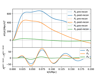
Figure 1: The multipoles of galaxy power spectra at $z=0.15$ for pre-reconstruction (dotted curves) and post-reconstruction (solid curves) cases. The differences between the two kinds of power spectra are shown in the lower panel.

A complete reconstructed power spectrum calculation can be found in Chen et al. (2019b). Here, we only adopt the form after decomposing the power spectrum into wiggle and no-wiggle parts. We use the method of splitting the power spectrum from Hinton et al. (2017). When we get a linear power spectrum, for example, it can be split as $P_{\mathrm{L}}(k)=P_{\mathrm{nw}}(k)+P_{\mathrm{w}}(k)$. For the reconstructed power spectrum, the no-wiggle parts reproduce the broadband depending on the linear power spectrum. And we can get the wiggle parts from Chen et al. (2019b) under some approximations, that we have

$$\begin{aligned} P^{dd}_{\mathrm{w}}(\mathbf{k})\approx&e^{-\frac{1}{2}K^{2}\Sigma_{dd}^{2}}\left[(1+f\mu^{2})(1-\mathcal{S}(k))+b_{1}\right]^{2}P_{\mathrm{w}}(k)\,,\\ P_{\mathrm{w}}^{ds}(\mathbf{k})=&-e^{-\frac{1}{2}K^{2}\Sigma_{ds}^{2}}\bigg{(}(1+f\mu^{2})(1-\mathcal{S}(k))+b_{1}\bigg{)}\\ &\times(1+f\mu^{2})\mathcal{S}(k)P_{\mathrm{w}}(k)\,,\\ P_{\mathrm{w}}^{ss}(\mathbf{k})=&e^{-\frac{1}{2}K^{2}\Sigma_{ds}^{2}}(1+f\mu^{2})^{2}\mathcal{S}(k)^{2}P_{\mathrm{w}}(k)\,,\end{aligned}$$ (13)

where $K^{2}=(1+f(f+2)\mu^{2})k^{2}$, the bias $b_{1}$ is relate to Eulerian bias by $b_{1}=b_{1}^{E}-1$, and $\Sigma_{dd}^{2}$, $\Sigma_{ds}^{2}$, $\Sigma_{ds}^{2}$ could also be found as (Ding et al., 2018)

$$\Sigma_{dd}^{2}(q,z)= \frac{2}{3}\int\frac{\mathrm{d}k}{2\pi^{2}}\left(1-j_{0}(q)\right)(1-S(k))^{2}P_{L}(k,z)\,,$$ (14)

$$\Sigma_{sd}^{2}(q,z)= \frac{2}{3}\int\frac{\mathrm{d}k}{2\pi^{2}}\left(\frac{1}{2}\left(S(k)^{2}+(1-S(k))^{2}\right)\right.$$

$$\left.+j_{0}(qk)(1-S(k))S(k)\right)P_{L}(k,z)\,,$$

$$\Sigma_{ss}^{2}(q,z)= \frac{2}{3}\int\frac{\mathrm{d}k}{2\pi^{2}}\left(1-j_{0}(qk)\right)S(k)^{2}P_{L}(k,z)\,.$$

Then, the reconstructed power spectrum is given by

$$\begin{aligned} P_{\mathrm{r}}=&\left[\left((1+f\mu^{2})(1-\mathcal{S}(k))+b_{1}\right)^{2}\left(P_{\mathrm{nw}}+e^{-\frac{1}{2}K^{2}\Sigma_{dd}^{2}}P_{\mathrm{w}}(k)\right)\right.\\ &+(1+f\mu^{2})^{2}\mathcal{S}(k)^{2}\left(P_{\mathrm{nw}}+e^{-\frac{1}{2}K^{2}\Sigma_{ds}^{2}}P_{\mathrm{w}}(k)\right)\\ &-2(1+f\mu^{2})\mathcal{S}(k)\bigg{(}(1+f\mu^{2})(1-\mathcal{S}(k))+b_{1}\bigg{)}\\ &\left.\left(P_{\mathrm{nw}}+e^{-\frac{1}{2}K^{2}\Sigma_{ds}^{2}}P_{\mathrm{w}}(k)\right)\right]\exp\left[-(k\mu\Sigma_{\mathrm{FoG}})^{2}\right].\end{aligned}$$ (15)

We show the multipoles of the pre-reconstruction and post-reconstruction galaxy power spectrum at $z=0.15$ in Fig. 1. The linear multipoles of the power spectra are calculated by CAMB (Lewis et al., 2000). Here, we also consider the Fingers-of-God (FoG) effect, and adopt a redshift-dependent value $\Sigma_{\rm FoG}=7/(1+z)\,h^{-1}\mathrm{Mpc}$ (Gong et al., 2019).

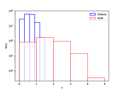
Figure 2: The expected galaxy and AGN redshift distributions in the CSST spectroscopic survey are shown in blue and red histograms, respectively. We divide the redshift ranges into five bins for these two surveys.

Table 1: The galaxy and AGN surface and volume number densities, and Eulerian biases in the five redshift bins for the CSST spectroscopic survey.

$z_{\rm min}$	$z_{\rm max}$	$z_{\rm mean}$	d$N$/d$\Omega{\rm[arcmin^{-2}]}$	$\bar{n}(z)[h^{3}{\rm Mpc^{-3}}]$	$b(z)$
			Galaxy
0	0.3	0.15	0.46	2.82 $\times 10^{-2}$	0.91
0.3	0.6	0.45	1.00	1.17 $\times 10^{-2}$	1.06
0.6	0.9	0.75	0.95	5.7 $\times 10^{-3}$	1.23
0.9	1.2	1.05	0.27	1.17 $\times 10^{-3}$	1.41
1.2	1.5	1.35	0.03	9.79 $\times 10^{-5}$	1.60
			AGN
0	1.0	0.5	1.72 $\times 10^{-2}$	3.85 $\times 10^{-5}$	1.20
1.0	2.0	1.5	3.67 $\times 10^{-2}$	2.85 $\times 10^{-5}$	2.31
2.0	3.0	2.5	2.09 $\times 10^{-2}$	1.39 $\times 10^{-5}$	3.98
3.0	4.0	3.5	3.65 $\times 10^{-3}$	2.23 $\times 10^{-6}$	6.20
4.0	5.0	4.5	1.11 $\times 10^{-4}$	5.99 $\times 10^{-8}$	8.98

3 Mock Data

Here, we consider two tracers of the matter density field, i.e. galaxy and AGN. The CSST spectroscopic observation can measure more than one hundred million galaxy spectra as shown in previous studies (e.g. Gong et al., 2019), and is also expected to identify millions of AGNs covering large redshift range, based on the CSST multi-band photometric survey.

3.1 Galaxy and AGN Mock Catalogs

For the CSST galaxy spectroscopic survey, we take the galaxy redshift distribution given in Gong et al. (2019) and Miao et al. (2023). It is created based on the zCOSMOS catalog (Lilly et al., 2007, 2009) in 1.7 $\mathrm{deg^{2}}$ with a magnitude limit $I_{\mathrm{AB}}\sim 22.5$. This catalog contains more than 20,000 galaxies, and about 16,600 sources have high-quality spectroscopic redshifts (spec-$z$). The derived galaxy surface and volume number densities of the CSST spectroscopic survey are listed in Table 1, and the galaxy redshift distribution is plotted in Figure 2. The galaxy distribution was given in five tomographic bins with a redshift range from 0 to 1.5.

For the AGN survey, CSST will significantly increase the number of observed AGNs by detecting and identifying them with the photometric and spectroscopic surveys. For calculating the expected number of AGN, we utilize the quasar luminosity function (QLF) from Palanque-Delabrouille et al. (2016). The QLF is given in g-band, which is often fitted by a double power law (Boyle et al., 2000; Richards et al., 2006):

$$\Phi\left(M_{g},z\right)=\frac{\Phi^{*}}{10^{0.4(\alpha+1)\left(M_{g}-M_{g}^{*}\right)}+10^{0.4(\beta+1)\left(M_{g}-M_{g}^{*}\right)}}\,,$$ (16)

where $M_{g}^{*}$ represents a characteristic or break magnitude. The slopes $\alpha$ and $\beta$ describe the evolution of the QLF on either side of the break magnitude. The slope $\alpha$ reproduces the bright end part of the QLF, and $\beta$ is for the faint end. Here, we have chosen to convert all the AGNs and their selection functions to the absolute AB magnitude at a g-band wavelength,

$$M_{g}\left(z\right)=m-5\log\left(\frac{d_{L}\left(z\right)}{\text{Mpc}}\right)-25-K_{m,g}\left(z\right)\,,$$ (17)

where

$$d_{L}(z)=(1+z)\frac{c}{H_{0}}\int_{0}^{z}\frac{\mathrm{d}z^{\prime}}{\sqrt{\Omega_{\mathfrak{m}}(1+z^{\prime})^{3}+\Omega_{\Lambda}}}\,,$$ (18)

and $K_{m,g}\left(z\right)\$ is the $K$ correction (McGreer et al., 2013; Caditz, 2017). Considering the pure luminosity-evolution (PLE) model (Croom et al., 2009), a redshift dependence of the luminosity is introduced through an evolution in $M_{g}^{*}$ given by

$$M_{g}^{*}(z)=M_{g}^{*}\left(z_{\mathrm{p}}\right)-2.5\left[k_{1}\left(z-z_{\mathrm{p}}\right)+k_{2}\left(z-z_{\mathrm{p}}\right)^{2}\right]\,,$$ (19)

where $z_{\mathrm{p}}=2.2$ is a pivot redshift. The redshift-evolution parameters ($k_{1}$ and $k_{2}$) and the slopes parameters ($\alpha$ and $\beta$) could be different on either side of the pivot redshift. The PLE model contains ten free parameters $[\Phi^{*},M_{g}^{*}(z_{\mathrm{p}}),\alpha_{l},\beta_{l},k_{1l},k_{2l},\alpha_{h},\beta_{h},k_{1h},\mathrm{~{}and~{}}k_{2h}]$, which are fit using eBOSS data (Dawson et al., 2016). The best-fit values of these parameters are given in Palanque-Delabrouille et al. (2016) and corrected in Caditz (2017) due to the different k-correction. We use the corrected best-fit values that are given in Table  2.

Table 2: The values of the free parameters we adopt in the PLE models of the QLF.

Redshift	Parameters
range
	$M_{g}^{*}(z_{p})$	$\log(\Phi^{*})$
$0.68-5.0$	$-26.5{\scriptstyle\pm 0.04}$	$-5.81{\scriptstyle\pm 0.01}$
	$\alpha$	$\beta$	$k_{1}$	$k_{2}$
$0.68-2.2$	$-3.4{\scriptstyle\pm 0.19}$	$-1.53{\scriptstyle\pm 0.25}$	$-0.03{\scriptstyle\pm 0.02}$	$-0.35{\scriptstyle\pm 0.02}$
$2.2-5.0$	$-2.62{\scriptstyle\pm 0.12}$	$-1.48{\scriptstyle\pm 0.05}$	$-0.36{\scriptstyle\pm 0.04}$	$0.01{\scriptstyle\pm 0.03}$

Based on the above QLF, one can assess the number of observed AGNs by

$$N_{\rm AGN}=\int{\rm d}M_{g}\int{\rm d}z\,\Phi\,\frac{{\rm d}V}{{\rm d}z}\,,$$ (20)

where $M_{g}$ is the magnitude in the g-band. The comoving volume element $\frac{{\rm d}V}{{\rm d}z}$ is given by

$$\frac{\mathrm{d}V}{\mathrm{~{}d}z}=\frac{\mathrm{d}V}{\mathrm{~{}d}z\mathrm{~{}d}\Omega}\times A\times\frac{4\pi}{41253}\,,$$ (21)

where A is the survey area in $\mathrm{deg}^{2}$, and

$$\frac{\mathrm{d}V}{\mathrm{d}z\mathrm{d}\Omega}=\frac{c}{H_{0}}\frac{d_{L}^{2}\left(z\right)}{\left(1+z\right)^{2}\left[\Omega_{\mathrm{m}}\left(1+z\right)^{3}+\Omega_{\Lambda}\right]^{1/2}}\,,$$ (22)

represents the comoving volume element per unit solid angle. We find that more than four million AGNs can be identified by the CSST, and the AGN redshift distribution is plotted in Figure 2. The AGN surface and volume number densities at different redshift bins from $z=0$ to 4 are given in Table 1.

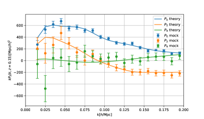
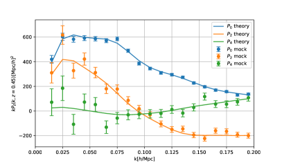
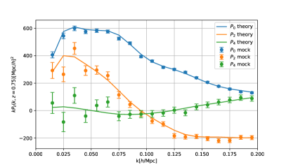
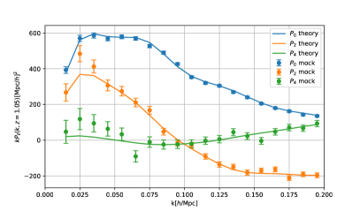
Figure 3: The mock data of multipoles of the galaxy post-reconstruction power spectra in four redshift bins from $z=0$ to 1.2 for the CSST spectroscopic survey. The corresponding theoretical power spectra are also shown as solid curves for comparison.

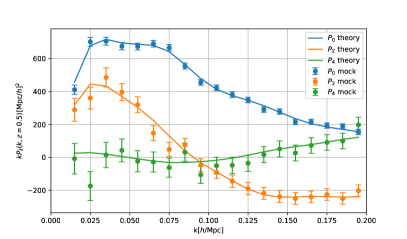
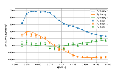
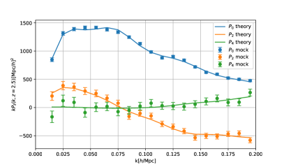
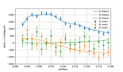
Figure 4: The mock data of the multipoles of the AGN power spectra in four redshift bins from $z=0$ to 4 for the CSST spectroscopic survey. The corresponding theoretical power spectra are also shown in solid curves for comparison.

3.2 BAO template

The BAO information can be derived by fitting the mock data of the galaxy and AGN power spectra in redshift space. For the CSST galaxy survey, we adopt the reconstructed power spectrum discussed in Sec. 2.3, and the smearing factor caused by the low spectral resolution of the slitless spectroscopic survey is also considered. The final galaxy power spectrum is then given by

$$P(k,\mu)=\exp\left[-(k\mu\sigma_{\mathrm{zerr}})^{2}\right]P_{\mathrm{r}}(k,\mu)\,,$$ (23)

where $\sigma_{\mathrm{zerr}}=\frac{c}{H(z)}\left(1+z\right)\sigma_{0,z}$, and $\sigma_{0,z}=0.002$ denotes the redshift accuracy of spectral calibration (Gong et al., 2019). We make use of the galaxy bias given by DESI Collaboration et al. (2016), and we have

$$b_{\mathrm{g}}(z)=\frac{0.84}{D(z)}\,,$$ (24)

where $D(z)$ is the growth factor. Note that $b_{\mathrm{g}}$ is the Eulerian bias, i.e. $b_{\mathrm{g}}=b_{1}^{E}$. We have listed the values of the galaxy biases in the five redshift bins in Table 1, and set them as free parameters in the fitting process.

For the AGN observation, as shown in Table 1, we can find that the volume number density is always $<10^{-4}\,h^{3}{\rm Mpc^{-3}}$ in the CSST spectroscopic survey. Given such low AGN number density, the reconstruction method probably cannot be used to restore the BAO feature as the case in the CSST galaxy survey (Neveux et al., 2020). So we would not adopt the reconstruction method in the AGN analysis, and then the AGN power spectrum can be modeled by

$$P(k,\mu)= (b_{A}+f\mu^{2})^{2}\exp\left[-(k\mu\sigma_{\mathrm{zerr}})^{2}\right]\exp\left[-(k\mu\Sigma_{\mathrm{FoG}})^{2}\right]$$ (25)

$$\left[P_{\mathrm{nw}}(k,\mu)+P_{\mathrm{w}}(k,\mu)e^{-\Sigma_{\mathrm{nl}}k^{2}}\right]\,,$$

where $\Sigma_{\mathrm{nl}}=\left(1-\mu^{2}\right)\Sigma_{\perp}^{2}/2+\mu^{2}\Sigma_{\parallel}^{2}/2$ denotes the anisotropic non-linear damping effect of the BAO, and we fix $\Sigma_{\perp}=8\,h^{-1}\mathrm{Mpc}$ and $\Sigma_{\parallel}=3\,h^{-1}\mathrm{Mpc}$ (Neveux et al., 2020). $b_{A}$ is the bias of AGN, and we take the form given in Laurent et al. (2017),

$$b_{\mathrm{A}}(z)=\alpha[(1+z)^{2}-6.565]+\beta\,,$$ (26)

with $\alpha=0.278$ and $\beta=2.3993$. The values of $b_{\mathrm{A}}$ in the five redshift bins can be found in Table 1, and we set them as free parameters when extracting the BAO signal.

To perform the measurements of the BAO scaling parameters, in general, a fiducial cosmology is adopted to measure the distances in radial and transverse directions. Then we can introduce the two scaling parameters in the two directions as

$$\begin{aligned} \alpha_{\parallel}(z)=\frac{D_{\mathrm{H}}(z)r_{\mathrm{drag}}^{\mathrm{ref}}}{D_{\mathrm{H}}^{\mathrm{ref}}(z)r_{\mathrm{drag}}}\,,\\ \alpha_{\perp}(z)=\frac{D_{\mathrm{M}}(z)r_{\mathrm{drag}}^{\mathrm{ref}}}{D_{\mathrm{M}}^{\mathrm{ref}}(z)r_{\mathrm{drag}}}\,.\end{aligned}$$ (27)

Here $D_{\mathrm{H}}\equiv c/H(z)$, $D_{\mathrm{M}}(z)$ is the comoving angular diameter distance, and ‘ref’ superscript represents the reference cosmology. The sound horizon, $r_{\mathrm{drag}}$, is determined by early-time physics and given by (Brieden et al., 2023).

$$r_{\mathrm{drag}} =\int_{\infty}^{z_{\mathrm{drag}}}\frac{c_{s}(z)}{H(z)}dz$$ (28)

$$\simeq\frac{147.05}{\mathrm{Mpc}}\left(\frac{\Omega_{\rm m}h^{2}}{0.1432}\right)^{-0.23}\left(\frac{N_{\mathrm{eff}}}{3.04}\right)^{-0.1}\left(\frac{\Omega_{\mathrm{b}}h^{2}}{0.02235}\right)^{-0.13}\,,$$

where $N_{\mathrm{eff}}$ is the effective number of neutrino species.

When we assume a reference cosmology that is different from the true cosmology, it will produce additional anisotropies, which is known as the AP effect (Alcock & Paczynski, 1979). It can be parametrized as

$$F_{\mathrm{AP}}(z)=F_{\epsilon}^{-1}(z)D_{\mathrm{M}}(z)^{\mathrm{ref}}/D_{\mathrm{H}}(z)^{\mathrm{ref}}\,,$$ (29)

where $F_{\epsilon}=\alpha_{\parallel}/\alpha_{\perp}$. Although the sound horizon $r_{\mathrm{drag}}$ is used as a reference scale, $F_{\mathrm{AP}}(z)$ is not dependent on it. Since the AP effect can distort the true wavenumbers of the power spectrum, the true wavenumbers $k_{\parallel}^{\prime}$ and $k_{\perp}^{\prime}$ are then related to the observed wavenumbers $k$ by $k_{\parallel}^{\prime}=k_{\parallel}/\alpha_{\parallel}$ and $k_{\perp}^{\prime}=k_{\perp}/\alpha_{\perp}$. Given the total wavenumber $k^{\prime}=\sqrt{k^{\prime}{}_{\parallel}^{2}+{k^{\prime}}_{\perp}^{2}}$ and the cosine of the angle to the line-of-sight $\mu$, we can write the relations between the true ($k^{\prime},\mu^{\prime}$) and observed values ($k,\mu$), that we have (Ballinger et al., 1996)

$$\begin{aligned} k^{\prime}=\frac{k}{\alpha_{\perp}}\left[1+\mu^{2}\left(\frac{1}{F_{\epsilon}^{2}}-1\right)\right]^{1/2}\,,\\ \mu^{\prime}=\frac{\mu}{F_{\epsilon}}\left[1+\mu^{2}\left(\frac{1}{F_{\epsilon}^{2}}-1\right)\right]^{-1/2}\,.\end{aligned}$$ (30)

Finally, the multipoles of the power spectrum are given by (Gil-Marín et al., 2020)

$$P_{\ell}(k)=\frac{2\ell+1}{2}\int_{-1}^{1}\mathrm{d}\mu\mathcal{L}_{\ell}(\mu)P[k^{\prime}(k,\mu),\mu^{\prime}(\mu)]+\sum_{i=1}^{n}A_{\ell,i}k^{i}\,.$$ (31)

Here the last term denotes a polynomial added to fit the broadband power spectrum, and we find 5th-order is good enough for fitting. Since we only focus on the BAO signal, we set the linear bias and the linear growth rate as free parameters, and the extra normalization factor $\frac{1}{\alpha_{\parallel}\alpha_{\perp}^{2}}$ is absorbed into the amplitude of the broadband power spectrum. Then we can generate the mock data of the power spectrum for monopole $P_{0}$, quadrupole $P_{2}$, and hexadecapole $P_{4}$. We create our mock data based on the Gaussian distribution, the mean value is given by the theoretical value, and the sigma is given by the square root of the diagonal elements of the covariance from Sec. 3.3.

3.3 Covariance Matrix

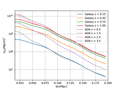
Figure 5: The effective volumes of the $P_{0}$ for the galaxy (solid curves) and AGN (dashed curves) in different redshift bins in the CSST spectroscopic surveys.

Generally, the covariance matrix can be estimated using analytical computation, simulation or observational data (Hamilton et al., 2006; Takahashi et al., 2009; Mohammed & Seljak, 2014; Mohammed et al., 2017; O’Connell & Eisenstein, 2019; Philcox et al., 2020a; Chudaykin & Ivanov, 2019; Wadekar & Scoccimarro, 2020; Wadekar et al., 2020; Hikage et al., 2020; Taruya et al., 2021; Mohammad & Percival, 2022; Philcox & Slepian, 2022; Hou et al., 2022; Ding et al., 2023b). Here we adopt the analytical computation method and estimate the covariance matrix by (Wadekar & Scoccimarro, 2020; Chudaykin & Ivanov, 2019),

$$C_{k_{i}k_{j}}^{(\ell_{1}\ell_{2})} =\delta_{ij}\frac{2}{N_{k}}\frac{(2\ell_{1}+1)}{2}\left(2\ell_{2}+1\right)$$ (32)

$$\times\int_{-1}^{1}d\mu L_{\ell_{1}}(\mu)L_{\ell_{2}}(\mu)\left[P(k_{i},\mu)+\frac{1}{\bar{n}}+N_{\mathrm{sys}}\right]^{2}\,,$$

where $N_{k}=V_{\mathrm{survey}}k^{2}dk/(4\pi^{2})$ is the number of modes, and $\bar{n}$ is the average source volume density. A potential systematical noise term $N_{\mathrm{sys}}$ is also considered (Gong et al., 2019), which can include the instrumental effects of the CSST slitless gratings, e.g. the success rate of achieving the required spec-$z$ accuracy. We will explore the results assuming $N_{\mathrm{sys}}=0$ and $10^{4}\,h^{-3}\,\mathrm{Mpc^{3}}$ as the optimistic and pessimistic cases, respectively.

In Figure 3 and Figure 4, we show the mock data of the multipoles of the galaxy post-reconstruction and AGN power spectra in different redshift bins for the CSST spectroscopic survey. Note that we do not use the mock data in the last redshift bins of the CSST galaxy and AGN surveys in the fitting process, since the number densities of galaxy and AGN are quite low in the two bins, as shown in Table 1. For the galaxy survey, the reconstruction cannot be performed in the redshift bin of $z$=1.2-1.5 with $\bar{n}_{\rm g}<10^{-4}\ h^{3}{\rm Mpc}^{-3}$. For the AGN survey, the density is less than $10^{-7}\ h^{3}{\rm Mpc}^{-3}$, and there is no effective measurement on the BAO signal in the redshift bin of $z$=3-4. For each of the other four redshift bins, we generate 19 data points from $k=0.015\,h/\mathrm{Mpc}$ to $0.195\,h/\mathrm{Mpc}$ with $\mathrm{d}k=0.01\,h/\mathrm{Mpc}$, and a random shift are added to each data point which is generated from a Gaussian distribution based on the covariance matrix.

We also calculate the effective volumes for the galaxy and AGN surveys in different redshift bins. The corresponding effective volume $V_{\mathrm{eff}}\equiv V_{\mathrm{survey}}\frac{P_{0}^{2}}{C^{(00)}}$ for the galaxies and AGNs, where $C^{(00)}$ is the diagonal element of the covariance matrix which contains the cosmic variance, shot noise and systematical noise. In Figure 5, we plot the corresponding effective volume for both the CSST galaxy and AGN spectroscopic surveys. We can see that our result is consistent with Gong et al. (2019) for the galaxy survey, and it is basically a factor of 3 larger compared to eBOSS surveys (Foroozan et al., 2021). On the other hand, the effective volume of AGN is comparable to the CSST galaxy survey, and even higher at large scales with $k<0.05\ h{\rm Mpc}^{-1}$. Therefore, we also expect to obtain precise BAO measurements in the CSST AGN spectroscopic survey.

4 Bayesian analysis

After obtaining the mock data of the multipole power spectra for the galaxy and AGN in the CSST spectroscopic surveys, we use the Markov Chain Monte Carlo (MCMC) method to fit the mock data and extract the BAO information. The Gaussian likelihood function can be written as

$$\mathcal{L}_{G}(\theta)\propto\mathrm{e}^{-\chi^{2}(\theta)/2}\,,$$ (33)

where $\theta$ denotes the model parameters, and $\chi^{2}(\theta)$ is given by

$$\chi^{2}(\theta)\equiv(P_{\ell}^{\mathrm{data}}-P_{\ell}^{\mathrm{model}})^{\mathrm{T}}C_{\rm P}^{-1}(P_{\ell}^{\mathrm{data}}-P_{\ell}^{\mathrm{model}})\,.$$ (34)

Here $C_{\rm P}$ is the covariance matrix of the mock data, which is given by Eq. (32), and the model and mock data vectors are composed of $\{P_{0}\,,P_{2}\,,P_{4}\}$, and the parameter vector $\theta$ stands for the 14 parameters in each redshift bin. Here we consider the two physical parameters, $\{\alpha_{\parallel},\alpha_{\perp}\}$, and 12 nuisance parameters,$\{b_{\rm g}\ {\rm or}\ b_{\rm A},f,A_{i}^{0},A_{i}^{2}\}$, where $f$ is the growth rate and $i=1,...5$ denotes the order of the polynomial. Note that we only consider the polynomial term in Eq. (31) for $P_{0}$ and $P_{2}$ here, and ignore it for $P_{4}$ since it is relatively small compared to the monopole and quadrupole power spectra.

Then, based on the extracted BAO information, i.e. $\alpha_{\parallel}$ and $\alpha_{\perp}$ derived from the above MCMC results, we also perform the Bayesian analysis of the cosmological parameters for exploring the constraint power. Here we investigate the constraints on the cosmological parameters for the $\Lambda$CDM and $w$CDM models. The $\chi^{2}$ is given by

$$\chi^{2}(\theta)\equiv\Sigma_{i}(D_{\mathrm{data}}-D_{\mathrm{model}})^{\mathrm{T}}C_{\rm D}^{-1}(D_{\mathrm{data}}-D_{\mathrm{model}})\,,$$ (35)

where $\Sigma_{i}$ represents the sum of all redshift bins, and the parameter vector $\theta$ stands for the cosmological parameters i.e. $\theta=\{h,\Omega_{\mathrm{m}},w,\Omega_{\mathrm{b}}h^{2}\}$. Here we adopt the prior information of baryon density from Big Bang nucleosynthesis (BBN), i.e. $\Omega_{\mathrm{b}}h^{2}=0.02235\pm 0.00037$ in our analysis (Schöneberg et al., 2019, 2022). The data vector $D_{\mathrm{data}}=\{\alpha_{\parallel},\alpha_{\perp}\}$, and the $D_{\mathrm{model}}$ can be estimated by Eq. (27). $C_{\rm D}$ is the covariance matrix for $\alpha_{\parallel}$ and $\alpha_{\perp}$ which can be derived from the MCMC chains. We use Cobaya (Torrado & Lewis, 2021) to complete the Bayesian inference, and set $R-1=0.005$ for the stopping criterion when generating chains. The first 30 percent of the chain points are removed in our analysis, and the rest chain points are used to generate the probability distribution of the parameters.

5 Results

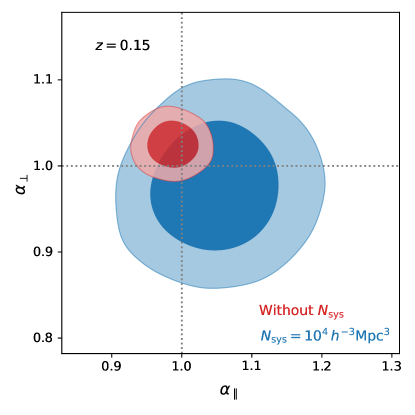
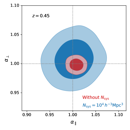
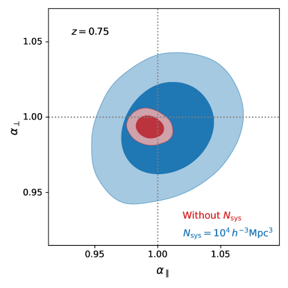
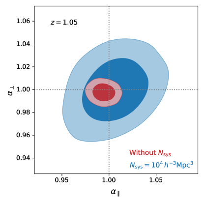
Figure 6: The predicted constraint results on the BAO scaling parameters in the CSST galaxy spectroscopic survey in the four redshift bins. The red and blue contours show the results assuming $N_{\rm sys}=0$ and $10^{4}\,h^{-3}\,\mathrm{Mpc^{3}}$ as the optimistic and pessimistic cases, respectively. The gray dotted lines denote the fiducial values.

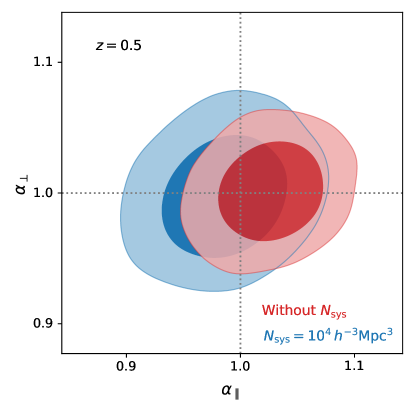
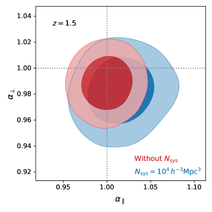
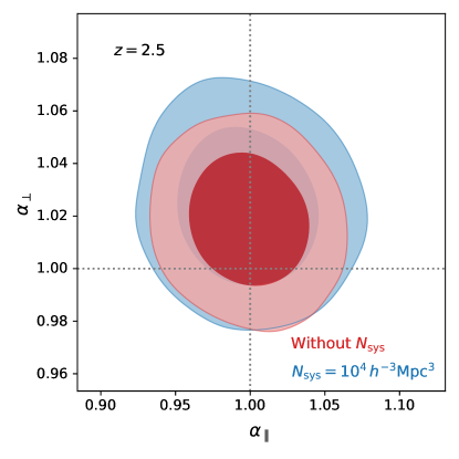
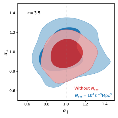
Figure 7: The predicted constraint results on the BAO scaling parameters in the CSST AGN spectroscopic survey in the four redshift bins. The red and blue contours show the results assuming $N_{\rm sys}=0$ and $10^{4}\,h^{-3}\,\mathrm{Mpc^{3}}$ as the optimistic and pessimistic cases, respectively. The gray dotted lines denote the fiducial values.

Table 3: The predicted best-fit values and 1$\sigma$ errors of $\alpha_{\parallel}$ and $\alpha_{\perp}$ from the CSST galaxy and AGN spectroscopic surveys. We have considered both the optimistic and pessimistic cases with $N_{\rm sys}=0$ and $10^{4}\,h^{-3}\,\mathrm{Mpc^{3}}$, respectively. The derived $D_{\mathrm{H}}/r_{\mathrm{drag}}$, $D_{\mathrm{M}}/r_{\mathrm{drag}}$, and reduce $\chi^{2}$ (57 data points and 14 parameters in each redshift bin) are also listed.

	$z_{\rm min}$	$z_{\rm max}$	$z_{\rm mean}$	$\alpha_{\parallel}$ (precision)	$\alpha_{\perp}$ (precision)	$D_{\mathrm{H}}/r_{\mathrm{drag}}$	$D_{\mathrm{M}}/r_{\mathrm{drag}}$	reduced $\chi^{2}$
Galaxy
$N_{\mathrm{sys}}=0$	0	0.3	0.15	$0.987\pm 0.024$ (2.4%)	$1.025\pm 0.018$ (1.8%)	$27.69\pm 0.67$	$4.48\pm 0.079$	1.28
	0.3	0.6	0.45	$1.0079\pm 0.0098$ (0.97%)	$0.9983\pm 0.0069$ (0.69%)	$23.79\pm 0.23$	$12.10\pm 0.084$	1.17
	0.6	0.9	0.75	$0.9936\pm 0.0074$ (0.74%)	$0.9934\pm 0.0050$ (0.5%)	$19.53\pm 0.15$	$18.47\pm 0.093$	1.51
	0.9	1.2	1.05	$0.9944\pm 0.0080$ (0.8%)	$0.9976\pm 0.0051$ (0.51%)	$16.34\pm 0.13$	$23.93\pm 0.122$	1.44
$N_{\mathrm{sys}}=10^{4}$	0	0.3	0.15	$1.050\pm 0.061$ (5.8%)	$0.976\pm 0.050$ (5.1%)	$29.45\pm 1.71$	$4.27\pm 0.22$	1.36
	0.3	0.6	0.45	$1.003\pm 0.028$ (2.8%)	$1.008\pm 0.022$ (2.2%)	$23.68\pm 0.66$	$12.21\pm 0.27$	1.20
	0.6	0.9	0.75	$1.007\pm 0.025$ (2.5%)	$0.993\pm 0.020$ (2.0%)	$19.80\pm 0.49$	$18.50\pm 0.37$	1.21
	0.9	1.2	1.05	$1.006\pm 0.023$ (2.3%)	$0.9996\pm 0.018$ (1.8%)	$16.53\pm 0.38$	$23.98\pm 0.43$	1.43
AGN
$N_{\mathrm{sys}}=0$	0	1.0	0.5	$1.026\pm 0.031$ (3.0%)	$1.001\pm 0.025$ (2.5%)	$23.50\pm 0.71$	$13.29\pm 0.33$	1.04
	1.0	2.0	1.5	$0.9999\pm 0.019$ (1.9%)	$0.989\pm 0.014$ (1.4%)	$12.79\pm 0.24$	$30.18\pm 0.43$	1.43
	2.0	3.0	2.5	$0.999\pm 0.027$ (2.7%)	$1.018\pm 0.017$ (1.7%)	$8.03\pm 0.22$	$41.38\pm 0.69$	1.10
	3.0	4.0	3.5	$1.007^{+0.097}_{-0.12}$ (11.4%)	$0.973^{+0.11}_{-0.089}$ (11.2%)	$5.63^{+0.54}_{-0.67}$	$46.07^{+5.21}_{-4.21}$	1.12
$N_{\mathrm{sys}}=10^{4}$	0	1.0	0.5	$0.986\pm 0.036$ (3.7%)	$0.998^{+0.029}_{-0.032}$ (3.1%)	$22.58\pm 0.83$	$13.26\pm 0.39$	1.15
	1.0	2.0	1.5	$1.016\pm 0.025$ (2.5%)	$0.982\pm 0.017$ (1.7%)	$13.0\pm 0.32$	$29.96\pm 0.52$	1.48
	2.0	3.0	2.5	$0.998\pm 0.031$ (3.1%)	$1.024\pm 0.02$ (2%)	$8.03\pm 0.25$	$41.62\pm 0.81$	1.26
	3.0	4.0	3.5	$0.97^{+0.11}_{-0.19}$ (16.0%)	$0.99^{+0.12}_{-0.16}$ (14.7%)	$5.42^{+0.61}_{-1.06}$	$46.87^{+5.68}_{-7.57}$	1.31

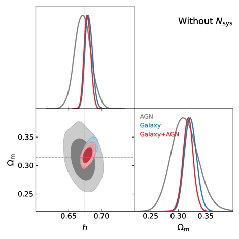
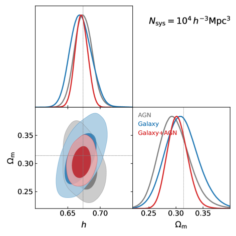
Figure 8: The predicted contour maps and 1D PDFs of $\Omega_{\rm m}$ and $h$ in the $\Lambda$CDM model for the CSST galaxy and AGN spectroscopic surveys. The constraint results by assuming $N_{\rm sys}=0$ and $10^{4}\,h^{-3}\,\mathrm{Mpc^{3}}$ are shown in the left and right panels, respectively. The gray, blue, and red contours and PDFs denote the results from the CSST galaxy, AGN, and joint surveys, respectively.

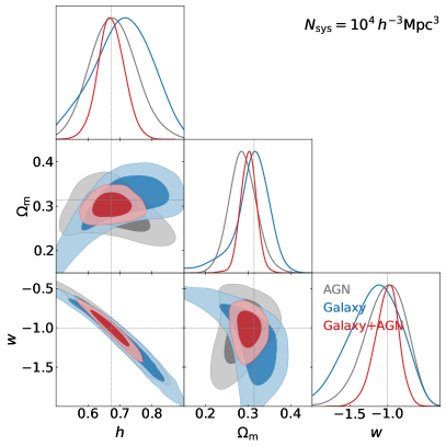
Figure 9: The predicted contour maps and 1D PDFs of $\Omega_{\rm m}$, $h$ and $w$ in the $w$CDM model for the CSST galaxy and AGN spectroscopic surveys. The constraint results by assuming $N_{\rm sys}=0$ and $10^{4}\,h^{-3}\,\mathrm{Mpc^{3}}$ are shown in the left and right panels, respectively. The gray, blue, and red contours and PDFs denote the results from the CSST galaxy, AGN, and joint surveys, respectively.

Table 4: The best-fit values and 1$\sigma$ errors of the relevant cosmological parameters in the $\Lambda$CDM and $w$CDM models derived from the mock BAO data ($\alpha_{\parallel}$ and $\alpha_{\perp}$) for the CSST galaxy and AGN spectroscopic surveys. The constraint results assuming $N_{\rm sys}=0$ and $10^{4}\,h^{-3}\,\mathrm{Mpc^{3}}$ are listed.

		$\Omega_{\mathrm{m}}$ (precision)	$H_{0}$ (precision)	w (precision)
$\Lambda$CDM
$N_{\mathrm{sys}}=0$	Galaxy BAO + BBN	$0.323^{+0.010}_{-0.012}$ (3.4%)	$68.07^{+0.51}_{-0.59}$ (0.81%)	-
	AGN BAO + BBN	$0.312^{+0.023}_{-0.026}$ (7.9%)	$67.2^{+1.1}_{-1.3}$ (1.9%)	-
	All BAO + BBN	$0.3182\pm 0.0094$ (3.0%)	$67.88^{+0.47}_{-0.53}$ (0.75%)	-
$N_{\mathrm{sys}}=10^{4}$	Galaxy BAO + BBN	$0.311^{+0.028}_{-0.032}$ (9.7%)	$67.0^{+1.5}_{-1.7}$ (2.4%)	-
	AGN BAO + BBN	$0.294^{+0.025}_{-0.030}$ (9.5%)	$67.4\pm 1.4$ (2.1%)	-
	All BAO + BBN	$0.302^{+0.016}_{-0.019}$ (5.9%)	$67.0\pm 0.99$ (1.5%)	-
$w$CDM
$N_{\mathrm{sys}}=0$	Galaxy BAO + BBN	$0.317^{+0.024}_{-0.013}$ (6.8%)	$67.7^{+4.3}_{-3.8}$ (6%)	$-0.99\pm 0.14$ (14%)
	AGN BAO + BBN	$0.295\pm 0.032$ (10.8%)	$71.5^{+6.6}_{-7.6}$ (9.8%)	$-1.19^{+0.34}_{-0.26}$ (24.4%)
	All BAO + BBN	$0.314^{+0.013}_{-0.011}$ (3.9%)	$66.7\pm 2.5$ (3.7%)	$-0.963^{+0.091}_{-0.079}$ (8.7%)
$N_{\mathrm{sys}}=10^{4}$	Galaxy BAO + BBN	$0.306^{+0.050}_{-0.026}$ (16.3%)	$70.6^{+10}_{-8.2}$ (13.2%)	$-1.16^{+0.38}_{-0.31}$ (28.6%)
	AGN BAO + BBN	$0.286\pm{0.032}$ (11.5%)	$67.9^{+6.4}_{-7.6}$ (10.7%)	$-1.03^{+0.31}_{-0.22}$ (26.7%)
	All BAO + BBN	$0.299\pm 0.019$ (6.5%)	$66.7\pm 4.1$ (6.2%)	$-0.995^{+0.17}_{-0.13}$ (16%)

We show the constraint results of $\alpha_{\parallel}$ and $\alpha_{\perp}$ for the CSST galaxy and AGN spectroscopic surveys in Figure 6 and 7, respectively. The best-fit values and 1$\sigma$ error of $\alpha_{\parallel}$, $\alpha_{\perp}$, and derived $D_{\mathrm{H}}/r_{\mathrm{drag}}$ and $D_{\mathrm{M}}/r_{\mathrm{drag}}$ in each redshift bin are also listed in Table 3. We investigate the constraint power with $N_{\rm sys}=0$ (red contours) and $10^{4}\,h^{-3}\,\mathrm{Mpc^{3}}$ (blue contours) as the optimistic and pessimistic cases, respectively.

We find that the constraint precision of the BAO scaling parameters can be higher than 1% and 3% at $0.3<z<1.2$ for the optimistic (without $N_{\rm sys}$) and pessimistic ($N_{\rm sys}=10^{4}\,h^{-3}\,\mathrm{Mpc^{3}}$) cases in the CSST galaxy spectroscopic survey. In $z<0.3$, the precision becomes lower by a factor of $\sim 2$ because of the small effective volume as shown in Figure 5. The constraint on $\alpha_{\perp}$ is basically better than $\alpha_{\parallel}$, due to the relatively low precision of spectroscopic redshift measured by the CSST slitless gratings. Our result is also consistent with that given by Ding et al. (2023a), where they predict the measurement precisions of $H(z)r_{\mathrm{drag}}$ and $D_{\mathrm{M}}/r_{\mathrm{drag}}$ in the CSST spectroscopic and photometric surveys. Compared to the current measurements, e.g. eBOSS (Gil-Marín et al., 2020), our result indicates that the CSST galaxy spectroscopic survey can effectively probe the BAO signal at higher redshifts up to $z\simeq 1.2$. Besides, it could improve the precision of the BAO measurement by a factor of $\sim$3 at least in the optimistic case, and can achieve similar precision in the pessimistic case.

We notice that, as shown in Figure 6, there is about 1$\sigma$ deviation from the fiducial values for the best-fits of the BAO scaling parameters in some redshift bins in the optimistic case (red contours). This is due to the Gaussian random shifts we add to the mock data (as shown in Figure 3) and degeneracies with the nuisance parameters, such as $b_{\rm g}$ and $A_{i}$. In the following discussions, we can see that this deviation is not statistically large enough to affect the constraints on the cosmological parameters.

In the CSST AGN spectroscopic survey, the precisions of the BAO measurements can be higher than 3% and 4% at $0<z<3$ for $N_{\rm sys}=0$ and $10^{4}\,h^{-3}\,\mathrm{Mpc^{3}}$, respectively. We can see that the effect of including $N_{\rm sys}$ is not as large as that in the CSST galaxy survey. This is because that the AGN power spectrum is higher than the galaxy power spectrum due to the larger AGN bias as shown in Figure 4, and it cannot significantly affect the AGN power spectrum by adding a $N_{\rm sys}$ around $10^{4}\,h^{-3}\,\mathrm{Mpc^{3}}$. At $3<z<4$, the constraint precision becomes much worse by a factor of $\sim 4$, which is due to a much lower AGN number density and effective volume as shown in Table 1 and Figure 5. When comparing our result with the current eBOSS measurements (Neveux et al., 2020), we can find that the CSST AGN spectroscopic survey can reach much higher redshift up to $z\sim 4$, and could improve the constraints on both $\alpha_{\parallel}$ and $\alpha_{\perp}$ by a factor of $\sim 2$ at least.

By making use of the mean values and covariance matrices of $\alpha_{\parallel}$ and $\alpha_{\perp}$ derived from the MCMC chains as the mock BAO data, we also explore the constraint power on the cosmological parameters in the $\Lambda$CDM and $w$CDM models. In Figure 8 and Figure 9, we show the contour maps and 1D probability distribution functions (PDFs) of the relevant cosmological parameters of the two models for $N_{\rm sys}=0$ and $10^{4}\,h^{-3}\,\mathrm{Mpc^{3}}$ cases in the CSST galaxy and AGN spectroscopic surveys.

For the $\Lambda$CDM model without considering $N_{\rm sys}$, we find that the constraint precisions of $\Omega_{\mathrm{m}}$ and $H_{0}$ can reach 3.4% and 0.81% in the CSST galaxy survey, respectively, and they are about 8% and 2% for the AGN survey. When combining both the galaxy and AGN data, we can further improve the constraint precisions to be 3% and 0.75%. After including $N_{\rm sys}=10^{4}\,h^{-3}\,\mathrm{Mpc^{3}}$, the parameter constraints become worse by a factor of $\sim$3 for the galaxy survey, $\sim$20% worse for the AGN survey, and a factor of $\sim$2 for the joint survey.

For the $w$CDM model, the constraint power becomes weaker for the cosmological parameters, especially for $H_{0}$, since an additional parameter $w$ is included. We find that, without $N_{\rm sys}$, the constraint precisions of $\Omega_{\mathrm{m}}$ and $H_{0}$ are 7% and 6% for the galaxy survey, 11% and 10% for the AGN survey, and 4% and 4% for the joint survey, respectively. When considering $N_{\rm sys}10^{4}\,h^{-3}\,\mathrm{Mpc^{3}}$, the precisions are worse by a factor of $\sim$2 for the galaxy survey, similar for the AGN survey, and 50% worse for the joint survey. The constraint precisions of $w$ are 14%, 24% and 9% for the galaxy, AGN and joint surveys, respectively, in the optimistic case without $N_{\rm sys}$, and 29%, 27% and 16% when considering $N_{\rm sys}=10^{4}\,h^{-3}\,\mathrm{Mpc^{3}}$ as the pessimistic case.

We also notice that the degeneracy directions of $\Omega_{\mathrm{m}}$ vs. $H_{0}$ are different for the CSST galaxy and AGN surveys in both Figure 8 and Figure 9. This is because that these two surveys mainly explore different redshift ranges, that $0<z\lesssim 1.2$ for the galaxy survey and $0<z\lesssim 4$ for the AGN survey, and the expansion of the Universe at $z\lesssim 1$ and $z>1$ are different, which are basically dominated by dark energy and dark matter, respectively. This can affect the degeneracy of $\Omega_{\mathrm{m}}$ vs. $H_{0}$, which is also indicated by previous studies (e.g. Alam et al., 2021). This indicates that the joint analysis of galaxies and AGNs can somehow break the degeneracy between parameters $w$ and $\Omega_{\mathrm{m}}$, and effectively improve the constraints.

6 Conclusions

In this work, we have studied the constraints on the BAO scaling parameters $\alpha_{\parallel}$ and $\alpha_{\perp}$ from the CSST galaxy and AGN spectroscopic surveys. We first forecast and generate the observed galaxy and AGN mock data of the multipole power spectra. For the galaxy survey, we perform reconstruction to reduce the non-linear effect on the BAO signal at $0<z<1.2$. For the AGN survey, we adopt the pre-reconstruction power spectra at $0<z<4$, since the AGN number density is too low to perform the reconstruction. We equally divided the redshift range into four bins for both of the CSST galaxy and AGN surveys. We find that more than one hundred million galaxies and four million AGNs will be observed by the CSST spectroscopic surveys.

Then we applied those mock power spectrum data to derive the BAO signal based on the BAO-only analysis by constraining the BAO scaling parameters, i.e. $\alpha_{\parallel}$ and $\alpha_{\perp}$. The MCMC technique is adopted to derive the constraint results. We explore the constraint power in the optimistic and pessimistic cases by excluding and including a systematical error $N_{\rm sys}$, which can account for the instrumental effects including the success rate of spec-$z$ accuracy. We find that the constraint precisions of $\alpha_{\parallel}$ and $\alpha_{\perp}$ can be higher than 1% and 3% for the galaxy and AGN surveys, respectively, in the optimistic case, which can improve the precision by a factor of 2-3 compared to the current measurements in the same redshift range. On the other hand, the CSST can provide similar constraint power as the current result in the pessimistic case, but can cover higher redshifts.

We also investigate the constraints on the cosmological parameters in the $\Lambda$CDM and $w$CDM models using the derived BAO data of $\alpha_{\parallel}$ and $\alpha_{\perp}$. We find that, for the $\Lambda$CDM model, the CSST joint galaxy and AGN spectroscopic surveys can provide stringent constraints on $\Omega_{\mathrm{m}}$ and $H_{0}$ with precisions $\sim$3% and 1%, respectively, in the optimistic case, and $\sim$6% and 1.5% in the pessimistic case. For the $w$CDM model including the dark energy equation of state $w$, the constraint precision becomes lower, especially for $H_{0}$ which is worse by a factor of $\sim$4, and it is 9% and 16% for $w$ in the optimistic and pessimistic cases, respectively. In addition, we only consider the case of CSST BAO measurements assisted by a prior of $\Omega_{\rm b}h^{2}$ from the BBN measurements. However, the constraint precision can be further improved by incorporating additional measurements, such as those from the CMB and the other CSST cosmological probes. This would enable unprecedented precise probing of the LSS as well as the properties of dark matter and dark energy.

Data Availability

The data that support the findings of this study are available from the corresponding author upon reasonable request.

References

- Akeson et al. (2019) Akeson R., et al., 2019, arXiv e-prints, p. arXiv:1902.05569
- Alam et al. (2017) Alam S., et al., 2017, MNRAS, 470, 2617
- Alam et al. (2021) Alam S., et al., 2021, Phys. Rev. D, 103, 083533
- Alcock & Paczynski (1979) Alcock C., Paczynski B., 1979, Nature, 281, 358
- Amendola et al. (2018) Amendola L., et al., 2018, Living Reviews in Relativity, 21, 2
- Anderson et al. (2012) Anderson L., et al., 2012, MNRAS, 427, 3435
- Anderson et al. (2014) Anderson L., et al., 2014, MNRAS, 441, 24
- Angulo et al. (2008) Angulo R. E., Baugh C. M., Frenk C. S., Lacey C. G., 2008, MNRAS, 383, 755
- Ata et al. (2018) Ata M., et al., 2018, MNRAS, 473, 4773
- Ballinger et al. (1996) Ballinger W. E., Peacock J. A., Heavens A. F., 1996, MNRAS, 282, 877
- Bargiacchi et al. (2022) Bargiacchi G., Benetti M., Capozziello S., Lusso E., Risaliti G., Signorini M., 2022, MNRAS, 515, 1795
- Bautista et al. (2021) Bautista J. E., et al., 2021, MNRAS, 500, 736
- Bernardeau et al. (2002) Bernardeau F., Colombi S., Gaztañaga E., Scoccimarro R., 2002, Phys. Rep., 367, 1
- Beutler et al. (2016) Beutler F., Blake C., Koda J., Marín F. A., Seo H.-J., Cuesta A. J., Schneider D. P., 2016, MNRAS, 455, 3230
- Beutler et al. (2017a) Beutler F., et al., 2017a, MNRAS, 464, 3409
- Beutler et al. (2017b) Beutler F., et al., 2017b, MNRAS, 466, 2242
- Blas et al. (2016) Blas D., Garny M., Ivanov M. M., Sibiryakov S., 2016, J. Cosmology Astropart. Phys., 2016, 028
- Boyle et al. (2000) Boyle B. J., Shanks T., Croom S. M., Smith R. J., Miller L., Loaring N., Heymans C., 2000, MNRAS, 317, 1014
- Brieden et al. (2023) Brieden S., Gil-Marín H., Verde L., 2023, J. Cosmology Astropart. Phys., 2023, 023
- Buchert (1989) Buchert T., 1989, A&A, 223, 9
- Buchert (1992) Buchert T., 1992, MNRAS, 254, 729
- Burden et al. (2014) Burden A., Percival W. J., Manera M., Cuesta A. J., Vargas Magana M., Ho S., 2014, MNRAS, 445, 3152
- Caditz (2017) Caditz D. M., 2017, A&A, 608, A64
- Carlson et al. (2013) Carlson J., Reid B., White M., 2013, MNRAS, 429, 1674
- Carrilho et al. (2023) Carrilho P., Moretti C., Pourtsidou A., 2023, J. Cosmology Astropart. Phys., 2023, 028
- Chen & Padmanabhan (2023) Chen X., Padmanabhan N., 2023, arXiv e-prints, p. arXiv:2311.09531
- Chen et al. (2019a) Chen S.-F., Castorina E., White M., 2019a, J. Cosmology Astropart. Phys., 2019, 006
- Chen et al. (2019b) Chen S.-F., Vlah Z., White M., 2019b, J. Cosmology Astropart. Phys., 2019, 017
- Chen et al. (2020) Chen S.-F., Vlah Z., White M., 2020, J. Cosmology Astropart. Phys., 2020, 062
- Chen et al. (2021) Chen S.-F., Vlah Z., Castorina E., White M., 2021, J. Cosmology Astropart. Phys., 2021, 100
- Chen et al. (2022a) Chen S.-F., Vlah Z., White M., 2022a, J. Cosmology Astropart. Phys., 2022, 008
- Chen et al. (2022b) Chen S.-F., White M., DeRose J., Kokron N., 2022b, J. Cosmology Astropart. Phys., 2022, 041
- Chudaykin & Ivanov (2019) Chudaykin A., Ivanov M. M., 2019, J. Cosmology Astropart. Phys., 2019, 034
- Chudaykin & Ivanov (2023) Chudaykin A., Ivanov M. M., 2023, Phys. Rev. D, 107, 043518
- Cole et al. (2005) Cole S., et al., 2005, MNRAS, 362, 505
- Crocce & Scoccimarro (2006) Crocce M., Scoccimarro R., 2006, Phys. Rev. D, 73, 063520
- Crocce & Scoccimarro (2008) Crocce M., Scoccimarro R., 2008, Phys. Rev. D, 77, 023533
- Croom et al. (2009) Croom S. M., et al., 2009, MNRAS, 392, 19
- DESI Collaboration et al. (2016) DESI Collaboration et al., 2016, arXiv e-prints, p. arXiv:1611.00036
- DESI Collaboration et al. (2023) DESI Collaboration et al., 2023, arXiv e-prints, p. arXiv:2306.06308
- Dawson et al. (2016) Dawson K. S., et al., 2016, AJ, 151, 44
- DeRose et al. (2023) DeRose J., Chen S.-F., Kokron N., White M., 2023, J. Cosmology Astropart. Phys., 2023, 008
- Desjacques et al. (2018) Desjacques V., Jeong D., Schmidt F., 2018, Phys. Rep., 733, 1
- Ding et al. (2018) Ding Z., Seo H.-J., Vlah Z., Feng Y., Schmittfull M., Beutler F., 2018, MNRAS, 479, 1021
- Ding et al. (2023a) Ding Z., Yu Y., Zhang P., 2023a, arXiv e-prints, p. arXiv:2305.00404
- Ding et al. (2023b) Ding J., Li S., Zheng Y., Luo X., Zhang L., Li X.-D., 2023b, arXiv e-prints, p. arXiv:2311.00981
- Eisenstein & Hu (1998) Eisenstein D. J., Hu W., 1998, ApJ, 496, 605
- Eisenstein et al. (2005) Eisenstein D. J., et al., 2005, ApJ, 633, 560
- Eisenstein et al. (2007a) Eisenstein D. J., Seo H.-J., White M., 2007a, ApJ, 664, 660
- Eisenstein et al. (2007b) Eisenstein D. J., Seo H.-J., Sirko E., Spergel D. N., 2007b, ApJ, 664, 675
- Foroozan et al. (2021) Foroozan S., Krolewski A., Percival W. J., 2021, J. Cosmology Astropart. Phys., 2021, 044
- Gil-Marín (2022) Gil-Marín H., 2022, J. Cosmology Astropart. Phys., 2022, 040
- Gil-Marín et al. (2016) Gil-Marín H., et al., 2016, MNRAS, 460, 4210
- Gil-Marín et al. (2020) Gil-Marín H., et al., 2020, MNRAS, 498, 2492
- Gong et al. (2019) Gong Y., et al., 2019, ApJ, 883, 203
- Hada & Eisenstein (2018) Hada R., Eisenstein D. J., 2018, MNRAS, 478, 1866
- Hamilton et al. (2006) Hamilton A. J. S., Rimes C. D., Scoccimarro R., 2006, MNRAS, 371, 1188
- Hikage et al. (2020) Hikage C., Takahashi R., Koyama K., 2020, Phys. Rev. D, 102, 083514
- Hinton et al. (2017) Hinton S. R., et al., 2017, MNRAS, 464, 4807
- Hivon et al. (1995) Hivon E., Bouchet F. R., Colombi S., Juszkiewicz R., 1995, A&A, 298, 643
- Hou et al. (2018) Hou J., et al., 2018, MNRAS, 480, 2521
- Hou et al. (2021) Hou J., et al., 2021, MNRAS, 500, 1201
- Hou et al. (2022) Hou J., Cahn R. N., Philcox O. H. E., Slepian Z., 2022, Phys. Rev. D, 106, 043515
- Hu & Sugiyama (1996) Hu W., Sugiyama N., 1996, ApJ, 471, 542
- Ivanov (2022) Ivanov M. M., 2022, arXiv e-prints, p. arXiv:2212.08488
- Ivanov et al. (2020) Ivanov M. M., Simonović M., Zaldarriaga M., 2020, J. Cosmology Astropart. Phys., 2020, 042
- Ivezić et al. (2019) Ivezić Ž., et al., 2019, ApJ, 873, 111
- Jeong & Komatsu (2006) Jeong D., Komatsu E., 2006, ApJ, 651, 619
- Jones et al. (2009) Jones D. H., et al., 2009, MNRAS, 399, 683
- Kazin et al. (2014) Kazin E. A., et al., 2014, MNRAS, 441, 3524
- Kokron et al. (2022) Kokron N., Chen S.-F., White M., DeRose J., Maus M., 2022, J. Cosmology Astropart. Phys., 2022, 059
- Laureijs et al. (2011) Laureijs R., et al., 2011, arXiv e-prints, p. arXiv:1110.3193
- Laurent et al. (2017) Laurent P., et al., 2017, J. Cosmology Astropart. Phys., 2017, 017
- Lewis et al. (2000) Lewis A., Challinor A., Lasenby A., 2000, ApJ, 538, 473
- Lilly et al. (2007) Lilly S. J., et al., 2007, ApJS, 172, 70
- Lilly et al. (2009) Lilly S. J., et al., 2009, ApJS, 184, 218
- Matsubara (2008a) Matsubara T., 2008a, Phys. Rev. D, 77, 063530
- Matsubara (2008b) Matsubara T., 2008b, Phys. Rev. D, 78, 083519
- Matsubara (2015) Matsubara T., 2015, Phys. Rev. D, 92, 023534
- McDonald & Roy (2009) McDonald P., Roy A., 2009, J. Cosmology Astropart. Phys., 2009, 020
- McGreer et al. (2013) McGreer I. D., et al., 2013, ApJ, 768, 105
- McQuinn & White (2016) McQuinn M., White M., 2016, J. Cosmology Astropart. Phys., 2016, 043
- Meiksin et al. (1999) Meiksin A., White M., Peacock J. A., 1999, MNRAS, 304, 851
- Merz et al. (2021) Merz G., et al., 2021, MNRAS, 506, 2503
- Miao et al. (2023) Miao H., Gong Y., Chen X., Huang Z., Li X.-D., Zhan H., 2023, MNRAS, 519, 1132
- Mohammad & Percival (2022) Mohammad F. G., Percival W. J., 2022, MNRAS, 514, 1289
- Mohammed & Seljak (2014) Mohammed I., Seljak U., 2014, MNRAS, 445, 3382
- Mohammed et al. (2017) Mohammed I., Seljak U., Vlah Z., 2017, MNRAS, 466, 780
- Neveux et al. (2020) Neveux R., et al., 2020, MNRAS, 499, 210
- Neveux et al. (2022) Neveux R., et al., 2022, MNRAS, 516, 1910
- Nikakhtar et al. (2021) Nikakhtar F., Sheth R. K., Zehavi I., 2021, Phys. Rev. D, 104, 043530
- Nikakhtar et al. (2022) Nikakhtar F., Sheth R. K., Lévy B., Mohayaee R., 2022, Phys. Rev. Lett., 129, 251101
- Nikakhtar et al. (2023) Nikakhtar F., Padmanabhan N., Lévy B., Sheth R. K., Mohayaee R., 2023, arXiv e-prints, p. arXiv:2307.03671
- Noh et al. (2009) Noh Y., White M., Padmanabhan N., 2009, Phys. Rev. D, 80, 123501
- O’Connell & Eisenstein (2019) O’Connell R., Eisenstein D. J., 2019, MNRAS, 487, 2701
- Ota et al. (2021) Ota A., Seo H.-J., Saito S., Beutler F., 2021, Phys. Rev. D, 104, 123508
- Ota et al. (2023) Ota A., Seo H.-J., Saito S., Beutler F., 2023, Phys. Rev. D, 107, 123523
- Padmanabhan et al. (2009) Padmanabhan N., White M., Cohn J. D., 2009, Phys. Rev. D, 79, 063523
- Padmanabhan et al. (2012) Padmanabhan N., Xu X., Eisenstein D. J., Scalzo R., Cuesta A. J., Mehta K. T., Kazin E., 2012, MNRAS, 427, 2132
- Palanque-Delabrouille et al. (2016) Palanque-Delabrouille N., et al., 2016, A&A, 587, A41
- Parkinson et al. (2012) Parkinson D., et al., 2012, Phys. Rev. D, 86, 103518
- Peebles & Yu (1970) Peebles P. J. E., Yu J. T., 1970, ApJ, 162, 815
- Percival et al. (2007) Percival W. J., Cole S., Eisenstein D. J., Nichol R. C., Peacock J. A., Pope A. C., Szalay A. S., 2007, MNRAS, 381, 1053
- Philcox & Ivanov (2022) Philcox O. H. E., Ivanov M. M., 2022, Phys. Rev. D, 105, 043517
- Philcox & Slepian (2022) Philcox O. H. E., Slepian Z., 2022, Proceedings of the National Academy of Science, 119, e2111366119
- Philcox et al. (2020a) Philcox O. H. E., Eisenstein D. J., O’Connell R., Wiegand A., 2020a, MNRAS, 491, 3290
- Philcox et al. (2020b) Philcox O. H. E., Ivanov M. M., Simonović M., Zaldarriaga M., 2020b, J. Cosmology Astropart. Phys., 2020, 032
- Philcox et al. (2021) Philcox O. H. E., Sherwin B. D., Farren G. S., Baxter E. J., 2021, Phys. Rev. D, 103, 023538
- Philcox et al. (2022) Philcox O. H. E., Farren G. S., Sherwin B. D., Baxter E. J., Brout D. J., 2022, Phys. Rev. D, 106, 063530
- Planck Collaboration et al. (2020) Planck Collaboration et al., 2020, A&A, 641, A6
- Raichoor et al. (2021) Raichoor A., et al., 2021, MNRAS, 500, 3254
- Richards et al. (2006) Richards G. T., et al., 2006, AJ, 131, 2766
- Ross et al. (2015) Ross A. J., Samushia L., Howlett C., Percival W. J., Burden A., Manera M., 2015, MNRAS, 449, 835
- Schmidt (2021) Schmidt F., 2021, J. Cosmology Astropart. Phys., 2021, 033
- Schmittfull et al. (2015) Schmittfull M., Feng Y., Beutler F., Sherwin B., Chu M. Y., 2015, Phys. Rev. D, 92, 123522
- Schmittfull et al. (2017) Schmittfull M., Baldauf T., Zaldarriaga M., 2017, Phys. Rev. D, 96, 023505
- Schöneberg et al. (2019) Schöneberg N., Lesgourgues J., Hooper D. C., 2019, J. Cosmology Astropart. Phys., 2019, 029
- Schöneberg et al. (2022) Schöneberg N., Verde L., Gil-Marín H., Brieden S., 2022, J. Cosmology Astropart. Phys., 2022, 039
- Semenaite et al. (2023) Semenaite A., et al., 2023, MNRAS, 521, 5013
- Senatore & Zaldarriaga (2015) Senatore L., Zaldarriaga M., 2015, J. Cosmology Astropart. Phys., 2015, 013
- Seo & Eisenstein (2005) Seo H.-J., Eisenstein D. J., 2005, ApJ, 633, 575
- Seo et al. (2008) Seo H.-J., Siegel E. R., Eisenstein D. J., White M., 2008, ApJ, 686, 13
- Seo et al. (2022) Seo H.-J., Ota A., Schmittfull M., Saito S., Beutler F., 2022, MNRAS, 511, 1557
- Sherwin & Zaldarriaga (2012) Sherwin B. D., Zaldarriaga M., 2012, Phys. Rev. D, 85, 103523
- Simon et al. (2022) Simon T., Zhang P., Poulin V., 2022, arXiv e-prints, p. arXiv:2210.14931
- Simon et al. (2023) Simon T., Zhang P., Poulin V., Smith T. L., 2023, Phys. Rev. D, 107, 123530
- Smith et al. (2020) Smith A., et al., 2020, MNRAS, 499, 269
- Springel et al. (2005) Springel V., et al., 2005, Nature, 435, 629
- Sunyaev & Zeldovich (1970) Sunyaev R. A., Zeldovich Y. B., 1970, Ap&SS, 7, 3
- Takahashi et al. (2009) Takahashi R., et al., 2009, ApJ, 700, 479
- Tamone et al. (2020) Tamone A., et al., 2020, MNRAS, 499, 5527
- Taruya et al. (2009) Taruya A., Nishimichi T., Saito S., Hiramatsu T., 2009, Phys. Rev. D, 80, 123503
- Taruya et al. (2021) Taruya A., Nishimichi T., Jeong D., 2021, Phys. Rev. D, 103, 023501
- Tassev (2014a) Tassev S., 2014a, J. Cosmology Astropart. Phys., 2014, 008
- Tassev (2014b) Tassev S., 2014b, J. Cosmology Astropart. Phys., 2014, 012
- Taylor & Hamilton (1996) Taylor A. N., Hamilton A. J. S., 1996, MNRAS, 282, 767
- Torrado & Lewis (2021) Torrado J., Lewis A., 2021, J. Cosmology Astropart. Phys., 2021, 057
- Vlah & White (2019) Vlah Z., White M., 2019, J. Cosmology Astropart. Phys., 2019, 007
- Vlah et al. (2015a) Vlah Z., Seljak U., Baldauf T., 2015a, Phys. Rev. D, 91, 023508
- Vlah et al. (2015b) Vlah Z., White M., Aviles A., 2015b, J. Cosmology Astropart. Phys., 2015, 014
- Vlah et al. (2016a) Vlah Z., Seljak U., Yat Chu M., Feng Y., 2016a, J. Cosmology Astropart. Phys., 2016, 057
- Vlah et al. (2016b) Vlah Z., Castorina E., White M., 2016b, J. Cosmology Astropart. Phys., 2016, 007
- Wadekar & Scoccimarro (2020) Wadekar D., Scoccimarro R., 2020, Phys. Rev. D, 102, 123517
- Wadekar et al. (2020) Wadekar D., Ivanov M. M., Scoccimarro R., 2020, Phys. Rev. D, 102, 123521
- Wang et al. (2017) Wang X., Yu H.-R., Zhu H.-M., Yu Y., Pan Q., Pen U.-L., 2017, ApJ, 841, L29
- Wang et al. (2020a) Wang Y., Li B., Cautun M., 2020a, MNRAS, 497, 3451
- Wang et al. (2020b) Wang Y., et al., 2020b, MNRAS, 498, 3470
- Weinberg et al. (2013) Weinberg D. H., Mortonson M. J., Eisenstein D. J., Hirata C., Riess A. G., Rozo E., 2013, Phys. Rep., 530, 87
- White (2005) White M., 2005, Astroparticle Physics, 24, 334
- White (2014) White M., 2014, MNRAS, 439, 3630
- White (2015) White M., 2015, MNRAS, 450, 3822
- Yu et al. (2017) Yu Y., Zhu H.-M., Pen U.-L., 2017, ApJ, 847, 110
- Zel’dovich (1970) Zel’dovich Y. B., 1970, A&A, 5, 84
- Zhan (2011) Zhan H., 2011, Scientia Sinica Physica, Mechanica & Astronomica, 41, 1441
- Zhan (2018) Zhan H., 2018, in 42nd COSPAR Scientific Assembly. pp E1.16–4–18
- Zhan (2021) Zhan H., 2021, Chinese Science Bulletin, 66, 1290
- Zhang et al. (2022) Zhang P., D’Amico G., Senatore L., Zhao C., Cai Y., 2022, J. Cosmology Astropart. Phys., 2022, 036
- Zhao et al. (2021) Zhao G.-B., et al., 2021, MNRAS, 504, 33
- Zhao et al. (2023) Zhao R., et al., 2023, arXiv e-prints, p. arXiv:2308.06206
- Zhu et al. (2017) Zhu H.-M., Yu Y., Pen U.-L., Chen X., Yu H.-R., 2017, Phys. Rev. D, 96, 123502
- d’Amico et al. (2020) d’Amico G., Gleyzes J., Kokron N., Markovic K., Senatore L., Zhang P., Beutler F., Gil-Marín H., 2020, J. Cosmology Astropart. Phys., 2020, 005
- de Mattia et al. (2021) de Mattia A., et al., 2021, MNRAS, 501, 5616
- von Hausegger et al. (2022) von Hausegger S., Lévy B., Mohayaee R., 2022, Phys. Rev. Lett., 128, 201302