Periodic finite-band solutions to the focusing nonlinear Schrödinger equation by the Riemann–Hilbert approach: inverse and direct problems

Abstract.

We consider the Riemann–Hilbert (RH) approach to the construction of periodic finite-band solutions to the focusing nonlinear Schrödinger (NLS) equation, addressing the question of how the RH problem parameters can be retrieved from the solution. Within the RH approach, a finite-band solution to the NLS equation is given in terms of the solution of an associated RH problem, the jump conditions for which are characterized by specifying the endpoints of the arcs defining the contour of the RH problem and the constants (so-called phases) involved in the jump matrices. In our work, we solve the problem of retrieving the phases given the solution of the NLS equation evaluated at a fixed time. Our findings are corroborated by numerical examples of phases computation, demonstrating the viability of the method proposed.

1. Introduction

About fifty years ago, the inverse scattering transform (IST) method was introduced. This method allows us to solve certain one-dimensional nonlinear evolution equations, called integrable equations, on the entire line of a spatial variable. This is achieved by analysing the corresponding linear problems constituting the associated Lax pair [1, 2, 3, 4].

The IST method can be divided into three main steps. (i) First, given the initial data, it involves solving a linear auxiliary set of equations and establishing a spectral (direct) problem. This spectral problem maps the initial data to a set of special quantities known as spectral data. (ii) Next, the method focuses on understanding the evolution of these spectral characteristics over time. (iii) Finally, it tackles an inverse problem, which allows retrieving the partial differential equation (PDE) solution at any desired value of time (evolution) variable.

For the initial value problems (for which the IST method was originally developed), where the data and the solution are assumed to vanish sufficiently fast as the spatial variable approach infinities, the direct spectral problem takes the form of a scattering problem. As for the inverse problem, the IST method in the original formulation uses the Gelfand–Levitan–Marchenko integral equations [5]. An alternative approach to the inverse problem is to consider a factorization problem of the Riemann–Hilbert (RH) type, formulated in the complex plane of the spectral parameter involved in the Lax pair equations [6].

The extension of the IST method to problems formulated on the half-line or on an interval proved to be a challenging task. A systematic approach to these problems known as the Unified Transform Method (a.k.a. the Fokas Method) was introduced by Fokas [7] and further developed by many researchers; see [8] and references therein. The method is based on the simultaneous spectral analysis of both equations of the Lax pair and the subsequent analysis of the so-called Global Relation coupling, in the spectral terms, the appropriate spectral transforms of the initial data and all boundary values. In certain cases of boundary conditions (called linearizable), the Global Relation can be “solved” in a way that allows us to formulate the associated RH problem in terms of the data for a well-posed problem alone.

In some recent papers [9, 10], it was shown that the initial boundary value problem on a finite interval $[0,L]\subset\mathbb{R}$ with $x$-periodic boundary conditions [$q(0,t)=q(L,t)$, $q_{x}(0,t)=q_{x}(L,t)$] for the nonlinear Schrödinger (NLS) equation, the focusing NLS,

$$iq_{t}+q_{xx}+2|q|^{2}q=0,$$ (1)

as well as the defocusing NLS belong to the class of linearizable problems: the solution $q(x,t)$ can be expressed in terms of the solution of an RH problem, the data for which (the jump matrix across a certain contour and the residue conditions) can be expressed in terms of the entries of the scattering matrix for a spectral problem on the whole line, associated with $q(x,0)$, $x\in[0,L]$ (continued by $0$ on ${\mathbb{R}}\setminus[0,L]$). Particularly, the contour for the RH problem is a union of the real and the imaginary axes and a number (possibly infinite) of finite segments symmetric w.r.t. the real axis.

The NLS equation is known to be a key model governing under specific conditions the signal propagation in single-mode optical fibres [11, 12]. The linearization of problems for the NLS equation provided by the IST method was the basis for the development of the nonlinear Fourier transform (NFT) based optical communication systems[11, 13]. The central idea of such an approach is to use, in order to carry the encoded data, the so-called nonlinear spectrum of a signal and to take advantage of the linear evolution of the spectrum. Most of the NFT-based optical communication systems studied so far deal with the rapidly-vanishing signals and suffer from the burst mode operation and high computational complexity of the involved processing elements, which reduces the practicality of the approach [11, 14]. Over recent years, there has been a growing interest in the development of optical communication methods based on the utilization of non-decaying solutions to the NLS equation [15, 16, 17, 18, 19, 20] as a more efficient alternative to the ”conventional“ NFT-based communications [21]. The IST operations associated with periodic finite-genus NLS solutions were named periodic nonlinear Fourier transform (PNFT) in these works. In Refs. [18, 19], an optical signal modulation and digital signal processing method has been proposed for a PNFT-based transmission, where the inverse problem step (the constructing of a signal in the physical domain at the transmitter side) harnesses the numerical solution to the RH problem.

The data for the RH the problem associated with the NLS equation are $2\times 2$ jump matrices, which are off-diagonal matrices satisfying a certain symmetry condition with constant entries on each separated part of the jump contour (consisting of a finite number of arcs). The solution of such an RH problem gives rise to a finite-band (finite-genus) solution to the NLS equation [22, 23]: the endpoints of the arcs fix the associated Riemann surface, while the constants in the jump matrices specify an individual solution. The present paper mainly addresses the direct part of the approach: given the profile $q(x,T)$ associated with some fixed $t=T$, recover the constants in the jump matrices of the RH problem generating $q(x,T)$ via the solution of an RH problem having the form as described above. We note that this direct problem for the general quasi-periodic solutions was solved approximately using neural networks in Ref. [24].

The outline of the paper is as follows. In Section 2, we review the inverse part consisting of generating a finite-band solution to the NLS equation by solving the RH problem with appropriate data (jump conditions). In Section 3, we briefly describe the ideas behind the development of the RH problem formalism for the periodic problem for the NLS equation presented in Refs. [9] and [10]. In Section 4, we present the details of the sequence of transformations of the RH problem leading to our main results on the direct problem stated in Theorems 4.3–4.5. The evolution of the spectral data is discussed in Section 5. Finally, in Section 6, we illustrate numerically the recovery of the phases (the constants in the jump matrices for the RH problem) using our direct problem algorithm.

2. The inverse problem by the RH approach

A wide variety of solutions of an integrable nonlinear evolution equation can be constructed in terms of solutions to a family of RH problems (parameterized by the independent variables of the nonlinear equation, say, $x$ and $t$) whose data depends on $x$ and $t$ in a way specific to the integrable nonlinear equation in question. Specifically, in the case of the focusing NLS equation (1), we have the following.

Proposition 2.1.

([22, 23]) Given $\{z_{j}\}_{0}^{N}$ with $\operatorname{Im}z_{j}>0$ and $\{\phi_{j}\}_{0}^{N}$ with $\phi_{j}\in[0,2\pi)$, define

• the oriented contour $\Sigma^{N}=\cup_{j=0}^{N}\Sigma_{j}$, where $\Sigma_{j}=(z_{j},\bar{z}_{j})$ (an arc connecting $z_{j}$ with $\bar{z}_{j}$), and

• the $2\times 2$-valued function

  $$J(x,t,z)=\begin{pmatrix}0&ie^{-i\phi_{j}-2izx-4iz^{2}t}\\ ie^{i\phi_{j}+2izx+4iz^{2}t}&0\end{pmatrix},\quad z\in\Sigma_{j}$$ (2)

and consider the following RH problem: find a $2\times 2$-valued function $\Psi(x,t,z)$ such that:

1. For all $x\in\mathbb{R}$ and $t\in\mathbb{R}$, $\Psi(x,t,z)$ is analytic w.r.t. $z$ for $z\in{\mathbb{C}}\setminus\bar{\Sigma}^{N}$ and continuous up to $\Sigma^{N}$ from the both sides of $\Sigma^{N}$;

2. The limiting values $\Psi^{+}(x,t,z)$ and $\Psi^{-}(x,t,z)$, $z\in\Sigma^{N}$ of $\Psi(x,t,z)$, as $z$ approaches $\Sigma^{N}$ from the $+$ and $-$ side respectively, are related by $J(x,t,z)$:

   $$\Psi^{+}(x,t,z)=\Psi^{-}(x,t,z)J(x,t,z),\qquad z\in\Sigma^{N};$$ (3)

3. At $z_{j}$ and $\bar{z}_{j}$, $\Psi(x,t,z)$ has the inverse fourth root singularities;

4. As $z\to\infty$,

   $$\Psi(x,t,z)=I+O(1/z),\qquad I=\left(\begin{smallmatrix}1&0\\ 0&1\end{smallmatrix}\right).$$ (4)

Then

1. For all $x$ and $t$, the RH problem (2)–(4) has a unique solutions $\Psi(x,t,z)$, which satisfies $\overline{\Psi(x,t,\bar{z})}=\sigma_{2}\Psi(x,t,z)\sigma_{2}$, where $\sigma_{2}=\left(\begin{smallmatrix}0&-i\\ i&0\end{smallmatrix}\right)$;

2. Defining $\Phi(x,t,z):=\Psi(x,t,z)e^{(-izx-2iz^{2}t)\sigma_{3}}$, where $\sigma_{3}=\left(\begin{smallmatrix}1&0\\ 0&-1\end{smallmatrix}\right)$, determining $\Psi_{1}(x,t)$ from $\Psi(x,t,z)=I+\frac{\Psi_{1}(x,t)}{z}+\dots$ as $z\to\infty$, and determining $q(x,t)$ by

   $$q(x,t)=2i[\Psi_{1}]_{12}(x,t)$$ (5)

   (where $[\cdot]_{12}$ stands for the $12$ entry of a matrix), we have:

   1. $q(x,t)$ is a solution of (1);

   2. $\Phi(x,t,z)$ satisfies the system of linear differential equations (Lax pair)

      $$\Phi_{x}=U\Phi$$ (6a)

      $$\Phi_{t}=V\Phi$$ (6b)

      with

      $$U(x,t,z)=-iz\sigma_{3}+\begin{pmatrix}0&q(x,t)\\ -\bar{q}(x,t)&0\end{pmatrix},$$ (7a)

      $$V(x,t,z)=-2iz^{2}\sigma_{3}+2z\begin{pmatrix}0&q(x,t)\\ -\bar{q}(x,t)&0\end{pmatrix}+\begin{pmatrix}i|q|^{2}&iq_{x}\\ i\bar{q}_{x}&-i|q|^{2}\end{pmatrix};$$ (7b)

3. $q(x,t)$ given by (5) is a solution of the NLS equation of finite-genus type: it can be expressed in terms of Riemann theta functions associated with the Riemann surface of genus $N$, with the branch points at $z_{j}$ and $\bar{z}_{j}$, $j=0,\dots,N$.

The last statement of Proposition 2.1 follows from the possibility to express $q(x,t)$ in terms of the solution of another RH problem (see Proposition 2.2 below), which can be considered as a transformation of the original RH problem evoking the so-called ”$g$-function mechanism“ [25, 26].

In order to formulate the modified RH problem, we need a set of parameters uniquely defined by the set of the branch points $z_{j}$ and $\bar{z}_{j}$, $j=0,\dots,N$. First, define $w(z)$ by

$$w(z)=\prod_{j=0}^{N}\sqrt{(z-z_{j})(z-\bar{z}_{j})}$$ (8)

as a function analytic in ${\mathbb{C}}\setminus\Sigma^{N}$ whose branch is fixed by the asymptotic condition $w(z)\simeq z^{N+1}$ as $z\to\infty$. Let each arc $\Sigma_{j}$ be oriented upward and let $w^{+}(z)$ be the values of $w$ at the “+” side of the corresponding $\Sigma_{j}$. Further, define the $N\times N$ matrix ${\mathbf{K}}$ by

$${\mathbf{K}}_{mj}:=\int_{\Sigma_{j}}\dfrac{\xi^{m-1}d\xi}{w^{+}(\xi)},\qquad m,j=1,\,\dots\,N,$$ (9)

and determine the vectors ${\mathbf{C}}^{f}:=(C^{f}_{1},\dots,C^{f}_{N})^{T}$ and ${\mathbf{C}}^{g}:=(C^{g}_{1},\dots,C^{g}_{N})^{T}$ as the solutions of the following linear equations:

$${\mathbf{K}}\cdot{\mathbf{C}}^{f}=\left[0,\dots,0,-2\pi i\right]^{T},\qquad{\mathbf{K}}\cdot{\mathbf{C}}^{g}=-4\pi i\left[0,\dots,0,2,\sum_{j=0}^{N}(z_{j}+\bar{z}_{j})\right]^{T},$$ (10)

(in the case $N=1$ or $N=2$, the last (respectively, two last) equations from (10) are to be considered).

Finally, determine the constants $f_{0}$ and $g_{0}$ from the large-$z$ developments of two scalar functions, $f(z)$ and $g(z)$, analytic in ${\mathbb{C}}\setminus\Sigma^{N}$:

$$f(z):=\frac{w(z)}{2\pi i}\sum_{j=1}^{N}\int_{\Sigma_{j}}\frac{C^{f}_{j}d\xi}{w^{+}(\xi)(\xi-z)}=z+f_{0}+O(1/z),$$ (11)

$$g(z):=\frac{w(z)}{2\pi i}\sum_{j=1}^{N}\int_{\Sigma_{j}}\frac{C^{g}_{j}d\xi}{w^{+}(\xi)(\xi-z)}=2z^{2}+g_{0}+O(1/z).$$ (12)

Proposition 2.2.

([23]) Given $\{z_{j}\}_{0}^{N}$ with $\operatorname{Im}z_{j}>0$ and $\{\phi_{j}\}_{0}^{N}$ with $\phi_{j}\in[0,2\pi)$, the genus-$N$ solution $q(x,t)$ of the NLS equation, which can be obtained as the solution of the RH problem of Proposition 2.1, can also be expressed by

$$q(x,t)=2i[\hat{\Phi}_{1}]_{12}(x,t)e^{2if_{0}x+2ig_{0}t},$$ (13)

where $\hat{\Phi}_{1}$ enters the large-$z$ development

$$\hat{\Phi}(x,t,z)=I+\frac{\hat{\Phi}_{1}(x,t)}{z}+\dots$$ (14)

of the solution $\hat{\Phi}(x,t,z)$ of the following RH problem: find $\hat{\Phi}(x,t,z)$ analytic in ${\mathbb{C}}\setminus\Sigma^{N}$ satisfying the jump conditions

$$\hat{\Phi}^{+}(x,t,z)=\hat{\Phi}^{-}(x,t,z)\hat{J}_{j}(x,t),\qquad z\in\Sigma_{j},\ j=0,\dots,N$$ (15)

with

$$\hat{J}_{j}(x,t)=\begin{pmatrix}0&ie^{-i(\phi_{j}+C^{f}_{j}x+C^{g}_{j}t)}\\ ie^{i(\phi_{j}+C^{f}_{j}x+C^{g}_{j}t)}&0\end{pmatrix}$$ (16)

and the normalization condition

$$\hat{\Phi}(x,t,z)=I+O(1/z),\qquad z\to\infty.$$ (17)

Here $C^{f}_{0}=C^{g}_{0}=0$ whereas the constants $f_{0}$ and $g_{0}$ in (13) and $C^{f}_{j}$, $C^{g}_{j}$, $j=1,\dots,N$ in (16) are determined by $\{z_{j}\}_{0}^{N}$ via (9)–(12).

Remark 2.1.

The solution $\Psi(x,t,z)$ of the RH problem in Proposition 2.1 is related to the solution $\hat{\Phi}(x,t,z)$ of the RH problem (15)–(17) as follows:

$$\Psi(x,t,z)=e^{(if_{0}x+ig_{0}t)\sigma_{3}}\hat{\Phi}(x,t,z)e^{(i(z-f(z))x+i(2z^{2}-g(z))t)\sigma_{3}}.$$ (18)

Remark 2.2.

It is the RH problem (15)–(17) that can be solved explicitly [22, 23], in terms of Riemann theta functions associated with the genus-$N$ Riemann surface associated with $w(z)$ (8) and characterized by the branch points $z_{j}$ and $\bar{z}_{j}$, $j=0,\dots,N$.

Remark 2.3.

If all $C^{f}_{j}$ together with $f_{0}$ turn to be commensurable, then the underlying solution of the NLS equation is periodic in $x$.

3. Direct problem in the periodic case: a sketch

The direct problem associated with the RH problem (2)–(4) (i.e., with the problem: given $\{\phi_{j}\}_{0}^{N}$, construct $q(x,t)$) consists in the following: given a $N$-genus solution $q(x,t)$ of the NLS equation associated with the prescribed branch points $\{{z}_{j}\}_{0}^{N}$ and evaluated as a function of $x$ at some fixed $t=t^{*}$, determine the underlying phase parameters $\phi_{j}$.

In the case where $C^{f}_{j}$ together with $f_{0}$ (see (10)–(12)) are commensurable and thus the underlying solution of the NLS equation is periodic in $x$, a possible way to solve the direct problem is based on the idea of finding a RH representation for the solution of the initial boundary value problem (IBVP) for the NLS equation, where the initial data given for $x$ varying on an interval (of the periodicity length $L$), i.e., $q(x,0)=q_{0}(x)$ for $x\in(0,L)$, are supplemented by the periodicity conditions:

$$q(0,t)=q(L,t),\quad q_{x}(0,t)=q_{x}(L,t)\quad\text{for all}\ t\geq 0.$$ (19)

If the RH problem in this representation had the same structure as the original RH problem (2)–(4), then the constants $\phi_{j}$ appearing in the jump construction would give the sought solution of our direct problem.

To get the appropriate representation, one can proceed in two steps: (i) first, provide some RH representation (with some contour and jumps), where the data for the RH problem can be constructed from the data of the periodic IBVP, i.e., the initial data $q_{0}(x)$ for $x\in(0,L)$; (ii) second, using the flexibility of the RH representation for the solution of nonlinear equations, transform this (original) RH problem to that having the above-mentioned desired form (2).

The first step has been recently addressed in [9] and [10], where it was shown that in the case (in particular) of the focusing NLS equation, the solution of the periodic IBVP (not necessarily finite-band) can be given in terms of the solution of a RH problem, where (i) the contour is the union of a (possibly infinite) number of finite arcs and the real and imaginary axes, and (ii) the jump matrices can be constructed in terms of the entries $a({z})$ and $b({z})$ of the scattering matrix:

$$s({z})=\begin{pmatrix}\overline{a(\bar{z})}&b({z})\\ -\overline{b(\bar{z})}&a({z})\end{pmatrix}\equiv\begin{pmatrix}a^{*}(z)&b({z})\\ -b^{*}(z)&a({z})\end{pmatrix},$$ (20)

where we adopt the notation $a^{*}(z)=\overline{a(\bar{z})}$ etc. Here $s(z)$ is the scattering matrix of the Zakharov–Shabat spectral problem (the $x$-equation of the Lax pair for the NLS equation) (6a) considered on the whole line, with the potential $q=q(x,0)$ involved in $U$ being continued on the whole line by setting it to $0$ for $x$ outside $[0,L]$.

To ensure the consistency of presentation, we briefly describe this step that can be performed in two sub-steps. In sub-step 1, an RH problem is constructed using the spectral functions $a({z})$ and $b({z})$ supplemented by the spectral functions $A({z})$, $B({z})$, $A_{1}({z})$, $B_{1}({z})$, that enter the scattering matrices

$$S({z})=\begin{pmatrix}A^{*}(z)&B({z})\\ -B^{*}(z)&A({z})\end{pmatrix},\qquad S_{1}({z})=\begin{pmatrix}A_{1}^{*}(z)&B_{1}({z})\\ -B_{1}^{*}(z)&A_{1}({z})\end{pmatrix}$$

associated with the $t$-equation from the Lax pair (6b) considered for $x=0$ and $x=L$ respectively [27, 28].

Namely, assuming for a moment that $q(0,t)$ and $q_{x}(0,t)$ are given for $t\in(0,T)$ with some $T>0$, Eq. (6b) can be considered, similarly to (6a), as a spectral problem for a matrix equation with coefficients determined in terms of $q(0,t)$ and $q_{x}(0,t)$, giving rise to $S(z)$ as the associated scattering matrix. Similarly, $q(L,t)$ and $q_{x}(L,t)$ give rise to $S_{1}(z)$. Then the periodicity condition (19) implies that $S(z)=S_{1}(z)$. Since $V$ in Eq. (6b) is a polynomial of the second order w.r.t. ${z}$, it follows that the contour where the scattering relation is established consists of two lines, the real and imaginary axes (where $\operatorname{Im}{z}^{2}=0$).

Since neither $q(0,t)$ nor $q_{x}(0,t)$ are given as the data for the periodic IBVP, sub-step 2 addresses the problem of replacing the RH problem constructed in terms of $a({z})$, $b({z})$, $A({z})$, and $B({z})$ by an equivalent one (in the sense that $q(x,t)$ obtained following (5) from the both problems are the same), whose formulation involves $a({z})$ and $b({z})$ only. A key for performing this sub-step is the so-called Global Relation [8, 9, 27, 28], which is a relation amongst $a({z})$, $b({z})$, $A({z})$, and $B({z})$ reflecting the fact that the IBVP with periodic boundary conditions is well-posed (particularly, has a unique solution) without prescribing the boundary values $q(0,t)$ and $q_{x}(0,t)$.

In the current setting (i.e., for the periodic problem in $x$), the global relation takes the form of the equation:

$$e^{2i{z}L}\left(A({z})a^{*}({z})+B({z})b^{*}({z})\right)B({z})+\left(A({z})b({z})-a({z})B({z})\right)A({z})=$$ (21)

$$=e^{4i{z}^{2}T}O\left(\frac{1+e^{2i{z}L}}{{z}}\right),$$

where the r.h.s. is not given precisely but only asymptotically, as ${z}\to\infty$. Noticing that the r.h.s. in (21) approaches $0$ as ${z}\to\infty$ staying in the first quadrant of the complex ${z}$-plane suggests replacing the r.h.s. by zero, which leads to a quadratic equation for the ratio $B({z})/A({z})$, with the coefficients given in terms of $a({z})$ and $b({z})$. Define $R({z})$ as the solution of the resulting equation,

$$e^{2izL}b^{*}(z)R^{2}(z)+\left(e^{2izL}a^{*}(z)-a(z)\right)R(z)+b(z)=0,$$ (22)

by

$$R({z})=\frac{e^{-i{z}L}a({z})-e^{i{z}L}a^{*}(z)+\sqrt{(e^{-i{z}L}a({z})-e^{i{z}L}a^{*}(z))^{2}-4b^{*}(z)b({z})}}{2e^{i{z}L}b^{*}(z)},$$ (23)

where the branch of the square root is chosen such that the branch cuts are the arcs connecting the pairs of complex conjugate points (actually, they are ${z}_{j}$ and $\bar{z}_{j}$) and that $R({z})\to 0$ as ${z}\to\infty$. Then, one can show that the RH problem sought in sub-step 2 is that obtained from the original RH problem, where $B({z})/A({z})$ is replaced by $R({z})$. Due to the jumps of $R({z})$ across the arcs connecting ${z}_{j}$ and $\bar{z}_{j}$, additional jump conditions on these arcs arise and thus the jump contour takes the form: $\cup_{j=0}^{N}\Sigma_{j}\cup{\mathbb{R}}\cup i{\mathbb{R}}$, whereas the jump matrix on all parts of the contour can be algebraically given in terms of $a({z})$, $b({z})$, and $R({z})$. To complete the formulation of the RH problem from step 1, the jump conditions have to be complemented by the residue conditions at the singularities of $R({z})$, if any (these are also given in terms of spectral quantities determined by the initial data only). For the exact formulation of the RH problem of step 1, see [10], Theorem 4.6 and Theorem 4.1 below.

Assumptions. In order to fix ideas while avoiding technicalities, we assume that (i) $a(z)$ has a finite number of simple zeros in the upper complex half-plane and these zeros do not coincide with the poles of $R({z})$ and $R^{*}({z})$ and (ii) $\operatorname{Re}z_{j}\neq 0$ for all $j$.

The second step consists of transforming the RH problem described above (with jumps across $\cup_{j=0}^{N}\Sigma_{j}\cup{\mathbb{R}}\cup i{\mathbb{R}}$ and residue conditions) to a RH problem of the form (2)–(4) with some constants $\phi_{j}$. We will show that this step can also be divided into several sub-steps: (i) transforming the RH problem to that with jumps across $\mathbb{R}$ and $i\mathbb{R}$ having the diagonal structure; (ii) reducing the jump conditions to those across $\Sigma^{N}=\cup_{j=0}^{N}\Sigma_{j}$ only and getting rid of singularity conditions; (iii) making the jumps on each $\Sigma_{j}$ to have the structure as in (2).

In the case $N=0$, this step has been done in [9, 10]; in this case, the contour for the RH problem consists of a single arc, and there are no singularity conditions. The associated ($0$-genus) solution of the NLS equation is a simple exponential function: $q(x,t)=\alpha e^{-2i\beta x+2i\omega t+i\phi_{0}}$, where $\alpha=\operatorname{Im}{z}_{0}$, $\beta=\operatorname{Re}{z}_{0}$, and $\omega=\alpha^{2}-2\beta^{2}$.

The cases with $N\geq 1$ turn out to be more involved. Particularly, in the realization of sub-step (ii) we need to get rid of singularity conditions at the singularity points of $R({z})$. In terms of the spectral theory of the Zakharov–Shabat equation with periodic coefficients, the (possibly empty) set of such singularity points $\{\mu_{j}\}_{1}^{N_{1}}$, $N_{1}\leq N$ consists of those conjugated auxiliary spectrum points for this problem which are located on the sheet (of the two-sheeted Riemann surface of $R$) characterized by the condition $R({z})\to 0$ as ${z}\to\infty$.

The resulting (${z}$-dependent) jump matrix is as follows:

$$\check{J}(x,t,{z})=\begin{pmatrix}0&iJ_{00}({z})e^{-2i{z}x-4i{z}^{2}t}\\ iJ_{00}^{-1}({z})e^{2i{z}x+4i{z}^{2}t}&0\end{pmatrix},\qquad{z}\in\Sigma^{N},$$ (24)

where $J_{00}({z})$ can be expressed in terms of $R(z)$ (see (100) below).

Having $J_{00}({z})$ obtained, sub-step (iii) can be done using the solution of the scalar RH problem:

$$d_{+}({z})d_{-}({z})=J_{00}({z})e^{i\phi_{j}},\quad{z}\in\Sigma_{j},\quad j=0,\,\dots,\,N,$$ (25)

$$d({z})\to 1,\quad{z}\to\infty.$$ (26)

In this problem, the constants $\phi_{j}$ are not prescribed but determined uniquely by (26) applied to the Cauchy-type solution of (25); they are the phases sought in the direct problem.

4. Direct problem in the periodic case: details

As we have mentioned above, using the ideas of the Unified Transform Method, it is possible to represent the solution of the periodic problem

$$iq_{t}+q_{xx}+2|q|^{2}q=0,\qquad x\in(0,L),\ t>0;$$ (27a)

$$q(x,0)=q_{0}(x),\qquad x\in[0,L];$$ (27b)

$$q(0,t)=q(L,t),\quad q_{x}(0,t)=q_{x}(L,t)\quad\text{for all}\ \,t\geq 0,$$ (27c)

in terms of the solution of an RH problem, the data for which (jump and residue conditions) can be constructed using the spectral functions $a(z)$ and $b(z)$ uniquely determined by the initial data $q_{0}(x)$. Namely, $a(z)$ and $b(z)$ are the entries of the scattering matrix $s(z)$ (20) relating the dedicated solutions $\Phi^{0}_{2}(x,z)$ and $\Phi^{0}_{3}(x,z)$ of the Zakharov–Shabat equation (6a), (7a) taken at $t=0$: let $U_{1}(x,0):=\begin{pmatrix}0&q_{0}(x)\\ -\bar{q}_{0}(x)&0\end{pmatrix}$; then $s(z)$ is determined by

$$\Phi^{0}_{3}(x,z)=\Phi^{0}_{2}(x,z)s(z),$$

where $\Phi^{0}_{2}(x,z)$ and $\Phi^{0}_{3}(x,z)$ are the solutions of the integral equations

$$\Phi^{0}_{2}(x,z) =e^{-izx\sigma_{3}}+\int_{0}^{x}e^{-iz(x-y)\sigma_{3}}U_{1}(y,0)\Phi^{0}_{2}(y,z)dy,$$

$$\Phi^{0}_{3}(x,z) =e^{-izx\sigma_{3}}-\int_{x}^{L}e^{-iz(x-y)\sigma_{3}}U_{1}(y,0)\Phi^{0}_{3}(y,z)dy.$$

In the construction of the associated RH problem, a key role is played by $R(z)$ (23). Before presenting this RH problem, we discuss some analytic properties of $R(z)$.

4.1. Analytic properties of $R(z)$

The scattering matrix $s({z})$ in our setting is closely related to the monodromy matrix $\mathcal{M}({z})$ of the Zakharov–Shabat equation with periodic conditions defined as $\mathcal{M}({z})=\Phi(L,0,{z})$, where $\Phi(x,0,{z})$ is the solution of Eq. (6a) satisfying the condition $\Phi(0,0,{z})=I$. Particularly, we have

$$\mathcal{M}_{11}(z)=\mathcal{M}^{*}_{22}(z)=e^{-izL}a(z),\quad\mathcal{M}_{12}(z)=-\mathcal{M}^{*}_{21}(z)=-e^{-izL}b(z).$$ (28)

In terms of $\mathcal{M}_{ij}$, equation (22) reads as

$$\mathcal{M}_{21}(z)R^{2}(z)+(\mathcal{M}_{22}(z)-\mathcal{M}_{11}(z))R(z)-\mathcal{M}_{12}(z)=0;$$ (29)

its solutions, $R_{(1)}({z})$ and $R_{(2)}({z})$, can be expressed as follows:

$$R_{(1)}({z})=\frac{\mathcal{M}_{11}({z})-\mathcal{M}_{22}({z})-\sqrt{\Delta^{2}({z})-4}}{2\mathcal{M}_{21}({z})}=\frac{e^{-izL}a(z)-e^{izL}a^{*}(z)-\sqrt{\Delta^{2}({z})-4}}{e^{izL}b^{*}(z)},$$ (30a)

$$R_{(2)}({z})=\frac{\mathcal{M}_{11}({z})-\mathcal{M}_{22}({z})+\sqrt{\Delta^{2}({z})-4}}{2\mathcal{M}_{21}({z})}=\frac{e^{-izL}a(z)-e^{izL}a^{*}(z)+\sqrt{\Delta^{2}({z})-4}}{e^{izL}b^{*}(z)},$$ (30b)

where

$$\Delta({z}):=\mathcal{M}_{11}({z})+\mathcal{M}_{22}({z})=e^{-izL}a(z)+e^{izL}a^{*}(z),$$ (31)

and we have used that

$$\det\mathcal{M}(z)=\mathcal{M}_{11}(z)\mathcal{M}_{22}(z)-\mathcal{M}_{12}(z)\mathcal{M}_{21}(z)=a^{*}(z)a(z)+b^{*}(z)b(z)\equiv 1.$$ (32)

As functions of $z$, $R_{(1)}({z})$ and $R_{(2)}({z})$ can be viewed as the branches of function $R$ meromorphic on the Riemann surface $(z,w)$ of

$$w^{2}=\prod\limits_{j=0}^{N}(z-z_{j})(z-\bar{z}_{j})$$

assuming that there is a finite number (denoted by $N+1$) of conjugated pairs $\{z_{j},\bar{z}_{j}\}$ of simple zeros of function $\Delta^{2}(z)-4$.

In the context of the spectral theory of the Zakharov–Shabat equation with periodic conditions, $\{{z}_{j},\bar{z}_{j}\}_{0}^{N}$ are called the main spectrum; they are the branch points of $R$. On the other hand, the simple zeros of $M_{12}({z})$ which are not double zeros of $\Delta^{2}({z})-4$ (as well as the multiple zeros of $\mathcal{M}_{12}({z})$) constitute the auxiliary spectrum $\{\mu_{j}\}_{1}^{N}$.

Notice that by the definition of $\mathcal{M}$, all zeros of $\mathcal{M}_{12}(z)$ are the eigenvalues of the homogeneous Dirichlet-type problem for the Zakharov–Shabat equation (6a) on $(0,L)$ with $q=q_{0}(x)$: if $\mathcal{M}_{12}(\tilde{z})=0$ for some $\tilde{z}$, then there exists a non-trivial vector solution $\Xi(x,\tilde{z})=(\Xi_{1}(x,\tilde{z}),\Xi_{2}(x,\tilde{z})^{T}$ of (6a) such that $\Xi_{1}(0,\tilde{z})=\Xi_{1}(L,\tilde{z})=0$ (actually, one can take $\Xi(x,\tilde{z})=\Phi^{(2)}(x,\tilde{z})$, where ${M}^{(l)}$ denote the $l$-th column of a $2\times 2$ matrix $M$).

Similarly, all zeros of $\mathcal{M}_{21}(z)$ are the eigenvalues of the homogeneous Neumann-type problem for the Zakharov–Shabat equation (6a) on $(0,L)$: for such $z$ there exists a non-trivial vector solution of (6a) such that its second component equals $0$ at $x=0$ and $x=L$.

One can view $R_{(1)}({z})$ and $R_{(2)}({z})$ as meromorphic functions on ${\mathbb{C}}\setminus\Sigma^{N}$ with the branch cut $\Sigma^{N}$, where $\Sigma^{N}=\cup_{0}^{N}\Sigma_{j}$ and $\Sigma_{j}$ are the vertical segment connecting $z_{j}$ and $\bar{z}_{j}$. Particularly, we specify $R_{(1)}({z})$ by the condition $R_{(1)}({z})\to 0$ as $z\to\infty$.

Let’s list some analytic properties of $R$ that hold for all $z$ including the limiting values at each side, $z_{+}$ and $z_{-}$, of $\Sigma_{j}(z)$:

1. By the definition of $R_{(1)}$ and $R_{(2)}$ (as the solutions of the quadratic equation),

   $$R_{(1)}({z})\cdot R_{(2)}({z})=-\frac{\mathcal{M}_{12}(z)}{\mathcal{M}_{21}(z)}=\frac{e^{-izL}b(z)}{e^{izL}b^{*}(z)};$$ (33)

   $$R_{(1)}(z)+R_{(2)}(z)=\frac{\mathcal{M}_{11}(z)-\mathcal{M}_{22}(z)}{\mathcal{M}_{21}(z)}=\frac{e^{-izL}a(z)-e^{izL}a^{*}(z)}{e^{izL}b^{*}(z)};$$ (34)

2. By the symmetries (28),

   $$R_{(2)}^{*}(z)=-\frac{1}{R_{(1)}(z)},$$ (35)

   (the both sides of (35) satisfy the same quadratic equation) and thus, in view of (33),

   $$\mathcal{M}_{21}(z)R(z)=\mathcal{M}_{12}(z)R^{*}(z)$$ (36)

   or

   $$e^{izL}b^{*}(z)R(z)=-e^{-izL}b(z)R^{*}(z),$$ (37)

   where $R(z)=R_{(1)}(z)$ or $R(z)=R_{(2)}(z)$.

3. $$\left(a(z)+b(z)R^{*}(z)\right)\left(a^{*}(z)+b^{*}(z)R(z)\right)\equiv 1.$$ (38)

   Indeed,

   $$\left(a+bR^{*}\right) \left(a^{*}+b^{*}R\right)=(\mathcal{M}_{11}-\mathcal{M}_{12}R^{*})(\mathcal{M}_{22}+\mathcal{M}_{21}R)=(\mathcal{M}_{11}-\mathcal{M}_{21}R)$$

   $$\times(\mathcal{M}_{22}+\mathcal{M}_{21}R)=1+\mathcal{M}_{12}\mathcal{M}_{21}-\mathcal{M}_{21}\left(\mathcal{M}_{21}R^{2}+(\mathcal{M}_{22}-\mathcal{M}_{11})R\right)$$

   $$=1-\mathcal{M}_{21}\left(\mathcal{M}_{21}R^{2}+(\mathcal{M}_{22}-\mathcal{M}_{11})R-\mathcal{M}_{12}\right)=1,$$

   where we have used (29), (32) and (37).

4. $$a(z)+b(z)R^{*}(z)\neq 0$$ (39)

   for all $z$. This follows from (38) and the fact that $b^{*}(z)R(z)$ is, by (30), non-singular.

   Actually, this also follows from the representation:

   $$a^{*}(z)+b^{*}(z)R(z)=\frac{1}{2}e^{-izL}(\Delta(z)\pm\sqrt{\Delta^{2}(z)-4}).$$

Finally, we list some properties of $R$ involving the limiting values at the different sides of $\Sigma_{j}(z)$ (denoting $R^{\pm}(z):=R(z_{\pm})$):

1. $\frac{R^{+}(z)}{R^{*+}(z)}=\frac{R^{-}(z)}{R^{*-}(z)}$ (follows from (36) and the fact that $M_{ij}(z)$ are entire functions).

2. $$R^{*+}(z)R^{-}(z)=R^{+}(z)R^{*-}(z)=-1$$ (40)

   (follows from (35) and ${R_{(2)}}(z_{+})={R_{(1)}}(z_{-})$, ${R_{(1)}}(z_{+})={R_{(2)}}(z_{-})$);

3. $$a^{*}(z)+b^{*}(z)R^{-}(z)=e^{-2izL}\bigl{(}a(z)+b(z)R^{*+}(z)\bigr{)}$$ (41)

   (follows from (40), (28) and (29) for $R^{-}$).

4.2. RH problem associated with the periodic problem for the NLS

From now on, we denote by $R(z)$ the branch in (30) decaying to $0$ as $z\to\infty$. Define $G(z)$, $G_{1}(z)$, and $G_{2}(z)$ as follows:

$$G(z)=-\frac{R^{*}(z)}{a(z)(a(z)+b(z)R^{*}(z))}=-\frac{R^{*}(z)}{a(z)}(a^{*}(z)+b^{*}(z)R(z))=-e^{-2izL}R^{*}(z)-\frac{b^{*}(z)}{a(z)},$$ (42)

$$G_{1}(z)=\frac{e^{2izL}a(z)R(z)}{a(z)+b(z)R^{*}(z)}=e^{2izL}a(z)R(z)(a^{*}(z)+b^{*}(z)R(z))=a^{2}(z)\left(R(z)-\frac{b(z)}{a(z)}\right),$$ (43)

$$G_{2}(z)=a^{-2}(z)G_{1}(z)=R(z)-\frac{b(z)}{a(z)}.$$ (44)

Using these functions, define a $2\times 2$ function $J_{0}(z)$ for $z\in{\mathbb{R}}\cup i{\mathbb{R}}\cup\Sigma^{N}$:

$$J_{0}(z)=\begin{cases}\begin{pmatrix}1&0\\ G_{2}^{*}(z)&1\end{pmatrix}\begin{pmatrix}1&\tilde{r}(z)\\ \tilde{r}^{*}(z)&1+|\tilde{r}|^{2}(z)\end{pmatrix}\begin{pmatrix}1&G_{2}(z)\\ 0&1\end{pmatrix},&z\in{\mathbb{R}}_{+},\\ \begin{pmatrix}1&G^{*}(z)\\ 0&1\end{pmatrix}\begin{pmatrix}1+|r|^{2}(z)&r^{*}(z)\\ r(z)&1\end{pmatrix}\begin{pmatrix}1&0\\ G(z)&1\end{pmatrix},&z\in{\mathbb{R}}_{-},\\ \begin{pmatrix}1&-G_{2}(z)\\ 0&1\end{pmatrix}\begin{pmatrix}a^{-1}(z)&0\\ 0&a(z)\end{pmatrix}\begin{pmatrix}1&0\\ G(z)&1\end{pmatrix},&z\in i{\mathbb{R}}_{+},\\ \begin{pmatrix}1&G^{*}(z)\\ 0&1\end{pmatrix}\begin{pmatrix}a^{*}(z)&0\\ 0&(a^{*}(z))^{-1}\end{pmatrix}\begin{pmatrix}1&0\\ -G_{2}^{*}(z)&1\end{pmatrix},&z\in i{\mathbb{R}}_{-},\\ \begin{pmatrix}1&R^{+}(z)-R^{-}(z)\\ 0&1\end{pmatrix},&z\in\Sigma^{N}\cap I,\\ \begin{pmatrix}1&0\\ e^{-2izL}({R^{*}}^{-}(z)-{R^{*}}^{+}(z))&1\end{pmatrix},&z\in\Sigma^{N}\cap II,\\ \begin{pmatrix}1&e^{2izL}({R}^{+}(z)-{R}^{-}(z))\\ 0&1\end{pmatrix},&z\in\Sigma^{N}\cap III,\\ \begin{pmatrix}1&0\\ {R^{*}}^{-}(z)-{R^{*}}^{+}(z)&1\end{pmatrix},&z\in\Sigma^{N}\cap IV,\end{cases}$$ (45)

where

$$r(z)=\frac{b^{*}(z)}{a(z)},\qquad\tilde{r}(z)=\frac{b(z)}{a(z)}.$$ (46)

Finally, specify the residue conditions for a $2\times 2$ function $M(x,t,z)$ at the poles of $R(z)$ and $R^{*}(z)$ as follows:

1. At the poles $\xi_{j}$ of $R(z)$ for $z\in I$:

   $$\underset{z=\xi_{j}}{\operatorname{Res}}M^{(2)}(x,t,z)=e^{-2i\xi_{j}x-4i\xi_{j}^{2}t}\underset{z=\xi_{j}}{\operatorname{Res}}R(z)M^{(1)}(x,t,\xi_{j}).$$ (47)

2. At the poles $\xi_{j}$ of $R^{*}(z)$ for $z\in II$:

   $$\underset{z=\xi_{j}}{\operatorname{Res}}M^{(1)}(x,t,z)=-e^{2i\xi_{j}(x-L)+4i\xi_{j}^{2}t}\underset{z=\xi_{j}}{\operatorname{Res}}R^{*}(z)M^{(2)}(x,t,\xi_{j}).$$ (48)

3. At the poles $\xi_{j}$ of $R(z)$ for $z\in III$:

   $$\underset{z=\xi_{j}}{\operatorname{Res}}M^{(2)}(x,t,z)=e^{-2i\xi_{j}(x-L)-4i\xi_{j}^{2}t}\underset{z=\xi_{j}}{\operatorname{Res}}R(z)M^{(1)}(x,t,\xi_{j}).$$ (49)

4. At the poles $\xi_{j}$ of $R^{*}(z)$ for $z\in IV$:

   $$\underset{z=\xi_{j}}{\operatorname{Res}}M^{(1)}(x,t,z)=-e^{2i\xi_{j}x+4i\xi_{j}^{2}t}\underset{z=\xi_{j}}{\operatorname{Res}}R^{*}(z)M^{(2)}(x,t,\xi_{j}).$$ (50)

Theorem 4.1.

Let $a(z)$ and $b(z)$ be the spectral functions associated with $q_{0}(x)$, $x\in(0,L)$ via the solution of the direct scattering problem for the Zakharov–Shabat equation (6a) with $q=q_{0}(x)$. Assume that (i) $a(z)$ has a finite number of simple zeros in ${\mathbb{C}}_{+}$ and (ii) the number of pairs $\{z_{j},\bar{z}_{j}\}$ of simple zeros of the function $\Delta^{2}(z)-4$, where $\Delta(z)$ is defined by (31), is finite. Introduce $\Sigma^{N}$ by $\Sigma^{N}=\cup_{0}^{N}\Sigma_{j}$, where $\Sigma_{j}$ is the vertical segment connecting $z_{j}$ and $\bar{z}_{j}$. Let $R(z)$ be determined by $a$ and $b$ via (30) such that $R(z)$ is analytic in ${\mathbb{C}}\setminus\Sigma^{N}$ and $R(z)\to 0$ as $z\to\infty$, and let $G(z)$ and $G_{2}(z)$ be determined in terms of $a$, $b$, and $R$ by (42) and (43).

Let $q(x,t)$ be defined by $q(x,t)=2i[M_{1}]_{12}(x,t)$, where $M(x,t,z)=I+\frac{M_{1}(x,t)}{z}+\dots$ as $z\to\infty$ and $M(x,t,z)$ is the solution of the Riemann–Hilbert problem specified by (i) the jump conditions

$$M^{+}(x,t,z)=M^{-}(x,t,z)J(x,t,z),\qquad z\in{\mathbb{R}}\cup i{\mathbb{R}}\cup\Sigma^{N},$$ (51)

where contour is oriented such that ${\mathbb{R}}$ is oriented from left to right, $i{\mathbb{R}}_{+}$ and $i{\mathbb{R}}_{-}$ are oriented towards infinities, and $\Sigma_{j}$ are oriented upwards, from $\bar{z}_{j}$ to $z_{j}$, and

$$J(x,t,z)=e^{-(izx+2iz^{2}t)\sigma_{3}}J_{0}(z)e^{(izx+2iz^{2}t)\sigma_{3}},$$ (52)

where $J_{0}$ is given by (45); (ii) the residue conditions (47)–(50), and (iii) the normalization condition $M(x,t,z)\to I$ as $z\to\infty$. Then $q(x,t)$ is the solution of the periodic problem (27).

Remark 4.1.

As we mentioned above, the construction of the RH problem in Theorem 4.1 is motivated by the application of the Unified Transform Method to the periodic problem [9, 10]. On the other hand, one can show directly that $q(x,t)$ obtained via the solution of this RH problem solves problem (27).

Particularly, one can prove that $q(x,t)$ (i) satisfies the initial conditions $q(x,0)=q_{0}(x)$ and (ii) satisfies the periodicity conditions (27c) by proving that (a) the jumps and the residue conditions for $t=0$ can be mapped to those in the RH problem associated with $q_{0}(x)$ and (b) the jumps and the residue conditions for $x=0$ and $x=L$ can be mapped to each other.

4.2.1. Verifying the initial conditions

Recall that the RH problem associated with $q_{0}(x)$ is as follows [27]: find $M^{(x)}(x,z)$ such that

1. $M^{(x)}(x,z)$ is meromorphic in ${\mathbb{C}}\setminus{\mathbb{R}}$ and satisfies the jump condition on $\Sigma^{(x)}:={\mathbb{R}}$:

   $$M^{(x)+}(x,z)=M^{(x)-}(x,z)J^{(x)}(x,z),\qquad z\in\Sigma^{(x)},$$ (53)

   where

   $$J^{(x)}(x,z):=e^{-izx\sigma_{3}}J_{0}^{(x)}(z)e^{izx\sigma_{3}},$$

   with

   $$J_{0}^{(x)}(z)=\begin{pmatrix}1+|r|^{2}(z)&r^{*}(z)\\ r(z)&1\end{pmatrix}.$$ (54)

2. Assuming that $a(z)$ has a finite number of simple zeros $\{\nu_{j}\}_{1}^{Q}$ in ${\mathbb{C}}_{+}$ (generic case), $M^{(x)}(x,z)$ satisfies the residue conditions

   $$\underset{z=\nu_{j}}{\operatorname{Res}}M^{(x)(1)}(x,z)=\frac{e^{2i\nu_{j}x}b^{*}(\nu_{j})}{\dot{a}(\nu_{j})}M^{(x)(2)}(x,\nu_{j}),$$ (55a)

   $$\underset{z=\bar{\nu}_{j}}{\operatorname{Res}}M^{(x)(2)}(x,z)=-\frac{e^{-2i\bar{\nu}_{j}x}b(\bar{\nu}_{j})}{\dot{a}^{*}(\bar{\nu}_{j})}M^{(x)(1)}(x,\bar{\nu}_{j}).$$ (55b)

3. $M^{(x)}(x,z)\to I$ as $z\to\infty$ for all $x\in(0,L)$.

Then $q_{0}(x)$ can be obtained by $q_{0}(x)=2i[M^{(x)}_{1}]_{12}(x)$, where $M_{1}^{(x)}(x)$ is involved in the large-$z$ development of $M^{(x)}(x,z)$: $M^{(x)}(x,z)=I+\frac{M_{1}^{(x)}(x)}{z}+\dots$.

Now we notice that the RH problem in Theorem 4.1 taken at $t=0$ can be mapped to the RH problem associated with $q_{0}(x)$ as follows:

$$M^{(x)}(x,z):=M(x,0,z)\cdot\begin{cases}\begin{pmatrix}a^{-1}(z)&0\\ 0&a(z)\end{pmatrix}\begin{pmatrix}1&-G_{1}(z)e^{-2izx}\\ 0&1\end{pmatrix},&z\in I,\\ \begin{pmatrix}1&0\\ -G(z)e^{2izx}&1\end{pmatrix},&z\in II,\\ \begin{pmatrix}1&G^{*}(z)e^{-2izx}\\ 0&1\end{pmatrix},&z\in III,\\ \begin{pmatrix}a^{*}(z)&0\\ 0&(a^{*})^{-1}(z)\end{pmatrix}\begin{pmatrix}1&0\\ G_{1}^{*}(z)e^{2izx}&1\end{pmatrix},&z\in IV.\end{cases}$$ (56)

Indeed:

1. By straightforward calculations, the jump for $M^{(x)}(x,z)$ across $\mathbb{R}$ is as in (53)–(54);

2. $M^{(x)}(x,z)$ has no jump across $\Sigma^{N}$.

3. All the off-diagonal entries in the r.h.s. of (56) go to $0$ exponentially fast as $z\to\infty$, $\operatorname{Im}z\neq 0$ for $x\in(0,L)$ (by the first expressions in (42) and (43) and since $R(z)\to 0$).

Now consider the mapping of the residue conditions.

(I) For $z\in I$: $M^{(x)}(x,z)=M(x,0,z)\begin{pmatrix}\frac{1}{a(z)}&-\frac{G_{1}(z)}{a(z)}e^{-2izx}\\ 0&a(z)\end{pmatrix}$.

1. At a zero $\nu_{j}$ of $a(z)$,

   $$M^{(x)(1)}(x,z)=M^{(1)}(x,0,z)\frac{1}{a(z)}=\frac{1}{z-\nu_{j}}C^{(1)}(x)+\dots.$$ (57)

   On the other hand, from $G_{1}(z)=-a(z)b(z)+a^{2}(z)R(z)$ it follows that as $z\to\nu_{j}$,

   $$G_{1}(z)=-\dot{a}(\nu_{j})(z-\nu_{j})b(\nu_{j})+O((z-\nu_{j})^{2})$$

   and thus

   $$M^{(x)(2)}(x,z)= -M^{(1)}(x,0,z)\frac{G_{1}(z}{a(z)}e^{-2izx}+a(z)M^{(2)}(x,0,z)$$ (58)

   $$=\frac{1}{z-\nu_{j}}C^{(1)}(x)\dot{a}(\nu_{j})(z-\nu_{j})b(\nu_{j})e^{-2i\nu_{j}x}+O(z-\nu_{j})$$

   $$=C^{(1)}(x)\dot{a}(\nu_{j})b(\nu_{j})e^{-2i\nu_{j}x}+O(z-\nu_{j}).$$

   It follows (also using $b(\nu_{j})=\frac{1}{b^{*}(\nu_{j})}$) that

   $$C^{(1)}(x)=e^{2i\nu_{j}x}\frac{b^{*}(\nu_{j})}{\dot{a}(\nu_{j})}M^{(x)(2)}(x,\nu_{j}).$$

   This, being combined with (57), gives

   $$\underset{z=\nu_{j}}{\operatorname{Res}}M^{(x)(1)}(x,z)=e^{2i\nu_{j}x}\frac{b^{*}(\nu_{j})}{\dot{a}(\nu_{j})}M^{(x)(2)}(x,\nu_{j}),$$

   which is the required residue condition (55a).

2. At a pole $\xi_{j}$ of $R(z)$,

   $$\underset{z=\xi_{j}}{\operatorname{Res}}M^{(x)(2)}(x,z)=-a(\xi_{j})\underset{z=\xi_{j}}{\operatorname{Res}}R(z)e^{-2i\xi_{j}x}M^{(1)}(x,0,\xi_{j})+a(\xi_{j})\underset{z=\xi_{j}}{\operatorname{Res}}M^{(2)}(x,0,z)$$

   $$=-a(\xi_{j})\underset{z=\xi_{j}}{\operatorname{Res}}R(z)e^{-2i\xi_{j}x}M^{(1)}(x,0,\xi_{j})+a(\xi_{j})\underset{z=\xi_{j}}{\operatorname{Res}}R(z)e^{-2i\xi_{j}x}M^{(1)}(x,0,\xi_{j})=0,$$

   where we have used (47).

(II) For $z\in II$: $M^{(x)}(x,z)=M(x,0,z)\begin{pmatrix}1&0\\ -G(z)e^{2izx}&1\end{pmatrix}$. In particular,

$$M^{(x)(2)}(x,\nu_{j})=M^{(2)}(x,0,\nu_{j}),$$

where $\nu_{j}$ is a zero of $a(z)$. On the other hand, by (42),

$$\underset{z=\nu_{j}}{\operatorname{Res}}G(z)=-\frac{b^{*}(\nu_{j})}{\dot{a}(\nu_{j})}$$

and thus

$$\underset{z=\nu_{j}}{\operatorname{Res}}M^{(x)(1)}(x,z) =-\underset{z=\nu_{j}}{\operatorname{Res}}G(z)e^{2i\nu_{j}x}M^{(2)}(x,0,\nu_{j})=-\frac{b^{*}(\nu_{j})}{\dot{a}(\nu_{j})}e^{2i\nu_{j}x}M^{(x)(2)}(x,\nu_{j}),$$

which is again the required residue condition (55a). Similarly for (55b).

Summarizing, transformation (56) produces $M^{(x)}(x,z)$ that satisfies the jump and residue conditions for the RH problem associated with $q_{0}(x)$, which implies that $q(x,0)=q_{0}(x)$.

4.2.2. Verifying the periodicity

In order to verify the periodicity, it is sufficient to relate the RH problem for $M(L,t,z)$ to that for $M(0,t,z)$ in such a way that both the jump residue conditions match correctly.

Introduce the piece-wise analytic matrix functions:

$$P^{(t)}(t,z)=\begin{cases}I,&z\in I\cup IV,\\ \begin{pmatrix}a(z)+b(z)R^{*}(z)&-b(z)e^{-4iz^{2}t}\\ 0&a^{*}(z)+b^{*}(z)R(z)\end{pmatrix},&z\in II,\\ \begin{pmatrix}a(z)+b(z)R^{*}(z)&0\\ b^{*}(z)e^{4iz^{2}t}&a^{*}(z)+b^{*}(z)R(z)\end{pmatrix},&z\in III,\end{cases}$$ (59)

and

$$\hat{P}^{(t)}(t,z)=\begin{cases}I,&z\in II\cup III,\\ \begin{pmatrix}a^{*}(z)+b^{*}(z)R(z)&0\\ -b^{*}(z)e^{2izL}e^{4iz^{2}t}&a(z)+b(z)R^{*}(z)\end{pmatrix},&z\in I,\\ \begin{pmatrix}a^{*}(z)+b^{*}(z)R(z)&b(z)e^{-2izL}e^{-4iz^{2}t}\\ 0&a(z)+b(z)R^{*}(z)\end{pmatrix},&z\in IV.\end{cases}$$ (60)

Then introduce

$$M^{(t)}(t,z):=M(0,t,z)P^{(t)}(t,z),\qquad\hat{M}^{(t)}(t,z):=M(L,t,z)\hat{P}^{(t)}(t,z).$$ (61)

Proposition 4.1.

$M^{(t)}(t,z)\equiv\hat{M}^{(t)}(t,z)$; consequently, $q(0,t)=q(L,t)$ and $q_{x}(0,t)=q_{x}(L,t)$ for all $t$.

To prove the proposition, it is sufficient to prove that $M^{(t)}(t,z)$ and $\hat{M}^{(t)}(t,z)$ satisfy the same jump and residue conditions.

1. Using the definitions of $R$, $G$ and $G_{2}$ as well as the properties (37) and (38) of $R$, it is by straightforward calculations that for $z\in{\mathbb{R}}\cup i{\mathbb{R}}$,

$$M^{(t)+}(t,z)=M^{(t)-}(t,z)J^{(t)}(t,z)\ \text{ and }\ \hat{M}^{(t)+}(t,z)=\hat{M}^{(t)-}(t,z)J^{(t)}(t,z)$$

involving the same $J^{(t)}(t,z)=\begin{pmatrix}1&R(z)e^{-4iz^{2}t}\\ R^{*}(z)e^{4iz^{2}t}&1+R^{*}(z)R(z)\end{pmatrix}$, where ${\mathbb{R}}\cup i{\mathbb{R}}$ is oriented such that quadrants I and III have positive boundaries.

2. Using, additionally, property (41), it follows that on parts of $\Sigma^{N}$, $J^{(t)}$ is given by

$$J^{(t)}(t,z)=\begin{cases}\begin{pmatrix}1&(R^{+}(z)-R^{-}(z))e^{-4iz^{2}t}\\ 0&1\end{pmatrix},&z\in I\cup III,\\ \begin{pmatrix}1&0\\ (R^{*+}(z)-R^{*-}(z))e^{4iz^{2}t}&1\end{pmatrix},&z\in II\cup IV.\end{cases}$$

3. In order to prove that $M^{(t)}(t,z)$ and $\hat{M}^{(t)}(t,z)$ satisfy the same residue conditions, we observe from (22) that if $\xi_{j}$ is a pole of $R(z)$, then $b^{*}(\xi_{j})=0$ and

$$\lim_{z\to\xi_{j}}b^{*}(z)R(z)=e^{-2izL}a(\xi_{j})-a^{*}(\xi_{j});$$ (62)

consequently,

$$(a^{*}+b^{*}R)|_{z=\xi_{j}}=e^{-2i\xi_{j}L}a(\xi_{j}),\qquad(a+bR^{*})|_{z=\xi_{j}}=e^{2i\xi_{j}L}a^{*}(\xi_{j}).$$ (63)

Similarly, if $\xi_{j}$ is a pole of $R^{*}(z)$, then $b(\xi_{j})=0$ and

$$\lim_{z\to\xi_{j}}b(z)R^{*}(z)=e^{2i\xi_{j}L}a^{*}(\xi_{j})-a(\xi_{j})$$ (64)

whereas (63) keep holding. Using these properties, it is again by straightforward calculations that $M^{(t)}(t,z)$ and $\hat{M}^{(t)}(t,z)$ satisfy the same residue conditions:

1. At the poles $\xi_{j}$ of $R(z)$ for $z\in I$ and $z\in III$:

   $$\underset{z=\xi_{j}}{\operatorname{Res}}M^{(t)(2)}(t,z)=e^{-4i\xi_{j}^{2}t}\underset{z=\xi_{j}}{\operatorname{Res}}R(z)M^{(t)(1)}(t,\xi_{j}).$$ (65)

2. At the poles $\xi_{j}$ of $R^{*}(z)$ for $z\in II$ and $z\in IV$:

   $$\underset{z=\xi_{j}}{\operatorname{Res}}M^{(t)(1)}(t,z)=-e^{4i\xi_{j}^{2}t}\underset{z=\xi_{j}}{\operatorname{Res}}R^{*}(z)M^{(t)(2)}(t,\xi_{j}).$$ (66)

4.3. From the basic RH problem to a RH problem with structure (2)-(4)

The reduction of the basic RH problem to the RH problem with structure (2)-(4) as in Proposition 2.1 can be performed in several consecutive steps.

In Step 1, we “undress” the jump matrices on ${\mathbb{R}}\cup i{\mathbb{R}}$ to those having a diagonal structure. This step will require appropriate algebraic factorizations of the jumps.

In Step 2, we reduce the RH problem obtained at Step 1 to that (i) with the contour $\Sigma^{N}$ only and (ii) having no residue conditions. This step will require analytic factorization of a scalar function.

In Step 3, we reduce the RH problem obtained at Step 2 to that having the structure as in Proposition 2.1, i.e., involving only constants $\phi_{j}$ as non-trivial elements in the construction of the jump matrices across $\Sigma^{N}$.

4.3.1. Step 1: Undressing the jump matrices on ${\mathbb{R}}\cup i{\mathbb{R}}$

Recall that in all our RH problem transformations involving multiplication from the right, we need that the diagonal part of the factors approaches the identity matrix as $z\to\infty$ (in all domains) whereas the off-diagonal parts decay exponentially fast to $0$ for all $t>0$ and all $x\in(0,L)$. Since the off-diagonal parts involve $e^{2izx+4iz^{2}t}$ or $e^{-2izx-4iz^{2}t}$, it follows that the appropriate factors should have triangular form, with a single non-zero off-diagonal entry containing the decaying exponential.

Introduce

$$D_{1}(z)=\frac{1}{1+R^{*}(z)R(z)},\quad D_{2}(z)=D_{1}^{-1}(z)=1+R^{*}(z)R(z),$$

$$D_{3}(z)=\frac{1+R^{*}(z)R(z)}{a(z)+b(z)R^{*}(z)},\quad D_{4}(z)=D_{3}^{*}(z)=\frac{1+R^{*}(z)R(z)}{a^{*}(z)+b^{*}(z)R(z)},$$

$$U(z)=-\frac{e^{2izL}R(z)}{1+R^{*}(z)R(z)},\quad L(z)=\frac{R^{*}(z)}{1+R^{*}(z)R(z)}.$$

Proposition 4.2.

The jump matrix $J_{0}(z)$ defined by (45) allows the following algebraic factorizations:

$$J_{0}(z)=\begin{cases}\begin{pmatrix}1&L^{*}(z)\\ 0&1\end{pmatrix}\begin{pmatrix}D_{1}(z)&0\\ 0&D_{1}^{-1}(z)\end{pmatrix}\begin{pmatrix}1&0\\ L(z)&1\end{pmatrix},&z\in{\mathbb{R}}_{+},\\ \begin{pmatrix}1&0\\ U^{*}(z)&1\end{pmatrix}\begin{pmatrix}D_{2}(z)&0\\ 0&D_{2}^{-1}(z)\end{pmatrix}\begin{pmatrix}1&U(z)\\ 0&1\end{pmatrix},&z\in{\mathbb{R}}_{-},\\ \begin{pmatrix}1&0\\ -L(z)&1\end{pmatrix}\begin{pmatrix}D_{3}(z)&0\\ 0&D_{3}^{-1}(z)\end{pmatrix}\begin{pmatrix}1&U(z)\\ 0&1\end{pmatrix},&z\in i{\mathbb{R}}_{+},\\ \begin{pmatrix}1&0\\ U^{*}(z)&1\end{pmatrix}\begin{pmatrix}D_{4}(z)&0\\ 0&D_{4}^{-1}(z)\end{pmatrix}\begin{pmatrix}1&-L^{*}(z)\\ 0&1\end{pmatrix},&z\in i{\mathbb{R}}_{-}.\end{cases}$$ (67)

Proof: by straightforward calculations.

Factorizations (67) suggest the undressing transformation of the RH problem as follows:

$$\tilde{M}(x,t,z)=M(x,t,z)\cdot\begin{cases}\begin{pmatrix}1&0\\ -L(z)e^{2izx+4iz^{2}t}&1\end{pmatrix},&z\in I\\ \begin{pmatrix}1&-U(z)e^{-2izx-4iz^{2}t}\\ 0&1\end{pmatrix},&z\in II\\ \begin{pmatrix}1&0\\ U^{*}(z)e^{2izx+4iz^{2}t}&1\end{pmatrix},&z\in III\\ \begin{pmatrix}1&L^{*}(z)e^{-2izx-4iz^{2}t}\\ 0&1\end{pmatrix},&z\in IV.\end{cases}$$ (68)

Notice that this transformation is appropriate in the sense that all the off-diagonal entries in the factors in (68) decay exponentially fast to $0$ as $z\to\infty$ for all $t>0$ and $x\in(0,l)$.

The jump conditions for $\tilde{M}$ across ${\mathbb{R}}\cup i{\mathbb{R}}$ involve obviously the diagonal matrices from the r.h.s. of (67). Concerning the jump conditions for $\tilde{M}$ across $\Sigma^{N}$ and the residue conditions for the RH problem for $\tilde{M}$, we have the following two propositions.

Proposition 4.3.

$\tilde{M}$ satisfies the following jump conditions across $\Sigma^{N}$:

$\tilde{M}^{+}(x,t,z)=\tilde{M}^{-}(x,t,z)\tilde{J}(x,t,z)$, where $\tilde{J}(x,t,z)=e^{-(izx+2iz^{2}t)\sigma_{3}}\tilde{J}_{0}(z)e^{(izx+2iz^{2}t)\sigma_{3}}$ with

$$\tilde{J}_{0}(z)=\begin{cases}\begin{pmatrix}0&R^{+}(z)-R^{-}(z)\\ \frac{1}{R^{-}(z)-R^{+}(z)}&0\end{pmatrix},&z\in\Sigma^{N}\cap I,\\ \begin{pmatrix}0&\frac{e^{2izL}}{R^{*+}(z)-R^{*-}(z)}\\ (R^{*-}(z)-R^{*+}(z))e^{-2izL}&0\end{pmatrix},&z\in\Sigma^{N}\cap II,\\ \begin{pmatrix}0&(R^{+}(z)-R^{-}(z))e^{2izL}\\ \frac{e^{-2izL}}{R^{-}(z)-R^{+}(z)}&0\end{pmatrix},&z\in\Sigma^{N}\cap III,\\ \begin{pmatrix}0&\frac{1}{R^{*+}(z)-R^{*-}(z)}\\ R^{*-}(z)-R^{*+}(z)&0\end{pmatrix},&z\in\Sigma^{N}\cap IV.\end{cases}$$ (69)

Proof. Consider $\Sigma^{N}\cap I$; here we have

$$\tilde{J}_{0}(z)= \begin{pmatrix}1&0\\ L^{-}&1\end{pmatrix}\begin{pmatrix}1&R^{+}-R^{-}\\ 0&1\end{pmatrix}\begin{pmatrix}1&0\\ -L^{+}&1\end{pmatrix}$$

$$=\begin{pmatrix}1&0\\ \frac{R^{*-}}{1+R^{*-}R^{-}}&1\end{pmatrix}\begin{pmatrix}1&R^{+}-R^{-}\\ 0&1\end{pmatrix}\begin{pmatrix}1&0\\ -\frac{R^{*+}}{1+R^{*+}R^{+}}&1\end{pmatrix}$$

$$=\begin{pmatrix}1&R^{+}-R^{-}\\ \frac{R^{*-}}{1+R^{*-}R^{-}}&1+\frac{(R^{+}-R^{-})R^{*-}}{1+R^{*-}R^{-}}\end{pmatrix}\begin{pmatrix}1&0\\ -\frac{R^{*+}}{1+R^{*+}R^{+}}&1\end{pmatrix}.$$

Now we notice that the $(22)$ entry in the first matrix equals $0$, because

$$1+R^{*-}R^{-}+(R^{+}-R^{-})R^{*-}=1+R^{*-}R^{-}+R^{+}R^{*-}-R^{-}R^{*-}=1+R^{+}R^{*-}=0$$ (70)

due to (40). It follows that

$$\tilde{J}_{0}(z)=\begin{pmatrix}1&R^{+}-R^{-}\\ \frac{R^{*-}}{1+R^{*-}R^{-}}&0\end{pmatrix}\begin{pmatrix}1&0\\ -\frac{R^{*+}}{1+R^{*+}R^{+}}&1\end{pmatrix}=\begin{pmatrix}0&R^{+}-R^{-}\\ \frac{1}{R^{-}-R^{+}}&0\end{pmatrix},$$

where we have again used the equality (70). Similarly for other quadrants.

Proposition 4.4.

$\tilde{M}$ satisfies the following singularity conditions:

1. For $z\in I\cup III$,

   $$\tilde{M}(x,t,z)=M_{reg}(x,t,z)\begin{pmatrix}z-\xi_{j}&0\\ 0&\frac{1}{z-\xi_{j}}\end{pmatrix}$$ (71)

   at all poles of $R(z)$ in $I\cup III$, where $M_{reg}$ is nowhere singular in $I\cup III$.

2. For $z\in II\cup IV$,

   $$\tilde{M}(x,t,z)=M_{reg}(x,t,z)\begin{pmatrix}\frac{1}{z-\xi_{j}}&0\\ 0&z-\xi_{j}\end{pmatrix}$$ (72)

   at all poles $\xi_{j}$ of $R^{*}(z)$ in $II\cup IV$, where $M_{reg}$ is nowhere singular in $II\cup IV$.

Remark 4.2.

The poles of $R^{*}(z)$ in $II\cup IV$ are complex conjugated to those of $R(z)$ in $I\cup III$.

Proof of Proposition 4.4. Consider $z\in I$, where $\tilde{M}=M\begin{pmatrix}1&0\\ -\frac{R^{*}}{1+R^{*}R}e^{2izx+4iz^{2}t}&1\end{pmatrix}$. It follows that $\tilde{M}^{(2)}=M^{(2)}$ and thus $\tilde{M}^{(2)}$ has the required singularity from (71) due to (47).

Now we need to show that $\tilde{M}^{(1)}(z)=O(z-\xi_{j})$ as $z\to\xi_{j}$. Indeed,

$$\tilde{M}^{(1)}(z) =M^{(1)}(z)-\frac{R^{*}(z)}{1+R^{*}(z)R(z)}e^{2izx+4iz^{2}t}M^{(2)}(z)=M^{(1)}(z)$$

$$-\frac{R^{*}(\xi_{j})}{1+R^{*}(\xi_{j})\left(\frac{\underset{z=\xi_{j}}{\operatorname{Res}}R(z)}{z-\xi_{j}}+O(1)\right)}\left(\frac{\underset{z=\xi_{j}}{\operatorname{Res}}R(z)}{z-\xi_{j}}M^{(1)}(\xi_{j})+O(1)\right)=O(z-\xi_{j}).$$

Similarly for other quadrants.

Looking at the diagonal factors in (67), we notice that we can simplify them getting rid of $a+bR^{*}$ and $a^{*}+b^{*}R$ by introducing

$$\hat{M}=\tilde{M}\cdot\begin{cases}I,&z\in II\cup III,\\ \begin{pmatrix}a^{*}+b^{*}R&0\\ 0&a+bR^{*}\end{pmatrix},&z\in I\cup IV.\end{cases}$$

Recall that $a+bR^{*}$ and $a^{*}+b^{*}R$ have neither zeros no singularities, and thus $\hat{M}$ satisfies the same singularity conditions as $\tilde{M}$.

On the other hand, the jump conditions for $\hat{M}$ on $\Sigma^{N}\cap I$ become:

$$\hat{J}_{0}=\begin{pmatrix}a+bR^{*-}&0\\ 0&a^{*}+b^{*}R^{-}\end{pmatrix}\begin{pmatrix}0&R^{+}(z)-R^{-}(z)\\ \frac{1}{R^{-}(z)-R^{+}(z)}&0\end{pmatrix}\begin{pmatrix}a^{*}+b^{*}R^{+}&0\\ 0&a+bR^{*+}\end{pmatrix}.$$ (73)

Using $(a+bR^{*-})(a^{*}+b^{*}R^{+})=e^{2izL}$ (see (41) and (38)), jump (73) becomes:

$$\hat{J}_{0}(z)=\begin{pmatrix}0&(R^{+}(z)-R^{-}(z))e^{2izL}\\ \frac{e^{-2izL}}{R^{-}(z)-R^{+}(z)}&0\end{pmatrix},\qquad z\in\Sigma^{N}\cap I,$$ (74)

which has the same form as for $z\in\Sigma^{N}\cap III$, see (69).

Similarly, the jump for $\hat{M}$ on $\Sigma^{N}\cap IV$ has the same expression as that for $\tilde{M}$ on $\Sigma^{N}\cap IV$, see (69).

Changing the orientation of ${\mathbb{R}}_{+}$ (setting it to go from $+\infty$ to $0$) and summarizing, we arrive at the following

Theorem 4.2.

Assuming that the number of the main spectrum points associated with $q_{0}(x)$ is finite, the solution $q(x,t)$ of the periodic IBVP (27) can be given by $q(x,t)=2i[\hat{M}_{1}]_{12}(x,t)$, where $\hat{M}_{1}(x,t)$ enters the large-$z$ development of $\hat{M}(x,t,z)$: $\hat{M}(x,t,z)=I+\frac{\hat{M}_{1}(x,t)}{z}+\dots$, and $\hat{M}(x,t,z)$ is the solution of the following RH problem: given $R(z)$ (which is constructed by (30) from the scattering coefficients $a(z)$ and $b(z)$ associated with the initial data $q_{0}(x)$, where the branch is chosen such that $R(z)\to 0$ as $z\to\infty$), find $\hat{M}(x,t,z)$ satisfying the following conditions:

1. $\hat{M}(x,t,z)$ is meromorphic in ${\mathbb{C}}\setminus({\mathbb{R}}\cup i{\mathbb{R}}\cup\Sigma^{N})$;

2. $\hat{M}(x,t,z)$ satisfies the jump conditions $\hat{M}^{+}(x,t,z)=\hat{M}^{-}(x,t,z)\hat{J}(x,t,z)$, where $\hat{J}(x,t,z)=e^{-(izx+2iz^{2}t)\sigma_{3}}\hat{J}_{0}(z)e^{(izx+2iz^{2}t)\sigma_{3}}$ and

   $$\hat{J}_{0}(z)=\begin{cases}\begin{pmatrix}1+R^{*}(z)R(z)&0\\ 0&\frac{1}{1+R^{*}(z)R(z)}\end{pmatrix},&z\in{\mathbb{R}}\cup i{\mathbb{R}},\\ \begin{pmatrix}0&(R^{+}(z)-R^{-}(z))e^{2izL}\\ \frac{e^{-2izL}}{R^{-}(z)-R^{+}(z)}&0\end{pmatrix},&z\in\Sigma^{N}\cap(I\cup III),\\ \begin{pmatrix}0&\frac{e^{2izL}}{R^{*+}(z)-R^{*-}(z)}\\ (R^{*-}(z)-R^{*+}(z))e^{-2izL}&0\end{pmatrix},&z\in\Sigma^{N}\cap(II\cup IV)\end{cases}$$ (75)

3. $\hat{M}(x,t,z)$ satisfies the singularity conditions (71) (for $z\in I\cup III$) and (72) (for $z\in II\cup IV$).

4. $\hat{M}(x,t,z)\to I$ as $z\to\infty$.

4.3.2. $R(z)$ in connection with the theory of periodic finite-band solutions of the NLS

Before passing to Step 2 (getting rid of jumps across ${\mathbb{R}}\cup i{\mathbb{R}}$ as well as of the singularity conditions), let us take a look at $R(z)$ taking into account the connection to the theory of finite-band periodic solutions (see, e.g., [29] and references therein).

Fix $(x_{0},t_{0})=(0,0)$ and denote $q=q(0,0)=q_{0}(0)$.

Proposition 4.5.

There exists an entire function $C(z)$ such that $\mathcal{M}_{12}(z)=C(z)g(z)$, $\mathcal{M}_{21}(z)=C(z)h(z)$, and $\frac{i}{2}(\mathcal{M}_{11}(z)-\mathcal{M}_{22}(z))=C(z)F(z)$, where

1. $g(z)=q\prod\limits_{j=1}^{N}(z-\mu_{j})$ and $h(z)=-\bar{q}\prod\limits_{j=1}^{N}(z-\bar{\mu}_{j})$;

2. The points $\{\mu_{j}\}_{1}^{N}$ constitutes the auxiliary spectrum (at $(x,t)=(0,0)$) of the Zakharov–Shabat operator (6a) with a periodic, finite-genus potential $q_{0}(x)$; it consists of the simple zeros of $\mathcal{M}_{12}(z)$ (or $b(z)$), which are not double zeros of $\Delta^{2}(z)-4$, where $\Delta(z)=\mathcal{M}_{11}(z)+\mathcal{M}_{22}(z)$, and of the multiple zeros of $\mathcal{M}_{12}(z)$, if any.

3. $F(z)$ is a polynomial such that the following relation holds:

   $$F^{2}(z)=P(z)+g(z)h(z),$$ (76)

   where $P(z)=w^{2}(z)=\prod\limits_{j=0}^{N}(z-z_{j})(z-\bar{z}_{j})$ and $z_{j}$ and $\bar{z}_{j}$ are simple zeros of $\Delta^{2}(z)-4$. This implies

   $$C^{2}(z)P(z)=\frac{1}{4}(4-\Delta^{2}(z)).$$ (77)

In view of Proposition 4.5, $R(z)$ can be expressed as follows:

• If $F(z)=z^{N+1}+\dots$, then (recalling that $\sqrt{P(z)}\sim z^{N+1}$ as $z\to\infty$)

  $$R(z)=R_{(1)}(z)=\frac{1}{\mathcal{M}_{21}(z)}\left(\frac{\mathcal{M}_{11}(z)-\mathcal{M}_{22}(z)}{2}-\sqrt{\frac{\Delta^{2}(z)}{4}-1}\right)$$ (78)

  $$=\frac{1}{C(z)h(z)}\left(-iC(z)F(z)+\sqrt{-C^{2}(z)P(z)}\right)=-\frac{i}{h(z)}(F(z)-\sqrt{P(z)}).$$

  Accordingly,

  $$R^{(1)*}(z)=-\frac{i}{g(z)}(F(z)-\sqrt{P(z)})$$ (79)

  (notice that $f^{*}=f$, $P^{*}=P$, $C^{*}=C$, $g^{*}=-h$) and

  $$R_{(2)}(z)=-\frac{1}{R^{(1)*}(z)}=-\frac{i}{h(z)}(F(z)+\sqrt{P(z)}).$$ (80)

• If $F(z)=-z^{N+1}+\dots$, then

  $$R_{(1)}(z)=-\frac{i}{h(z)}(F(z)+\sqrt{P(z)}).$$ (81)

Remark 4.3.

Concerning the singularity conditions in Theorem 4.2 we observe the following:

1. The set of poles of $R(z)$ consists of those zeros of $b^{*}(z)$ (i) which are zeros of $h(z)$ (i.e., belong to the conjugated auxiliary spectrum $\{\bar{\mu}_{j}\}_{1}^{N}$), and, at the same time, (ii) which are not zeros of $F(z)\mp\sqrt{P(z)}$ (or, in view of (76), are zeros of $F(z)\pm\sqrt{P(z)}$). Actually, the auxiliary spectrum $\{\bar{\mu}_{j}\}_{1}^{N}$ consists of all poles of $R$ as a function on the two-sheet Riemann surface (or, equivalently, the set of all poles of $R_{(1)}(z)$ and $R_{(2)}(z)$ as functions on the complex plane).

2. Not all poles of $R(z)$ are involved in the singularity conditions (only those in $I$ and $III$).

Consequently, in particular cases it is possible that there are no singularity conditions at all but in general, there can be up to $N$ singularity conditions in $I$ and $III$.

From (78),(79) and (81) it follows that

$$1+R^{*}(z)R(z)=\frac{2\sqrt{P(z)}}{\tilde{F}(z)+\sqrt{P(z)}},$$ (82)

where

$$\tilde{F}(z)=\begin{cases}F(z),&\text{if}\ F(z)=z^{N+1}+\dots,\\ -F(z),&\text{if}\ F(z)=-z^{N+1}+\dots.\end{cases}$$ (83)

Thus the zeros (of order $1/2$) of $1+R^{*}(z)R(z)$ are, generically, the branch points (the main spectrum points) $\{z_{j},\bar{z}_{j}\}_{0}^{N}$.

4.3.3. Step 2: getting rid of the jumps across ${\mathbb{R}}\cup i{\mathbb{R}}$ as well as of the singularities

Due to (75), one can get rid of jumps across ${\mathbb{R}}\cup i{\mathbb{R}}$ by multiplication from the right by diagonal matrices $\begin{pmatrix}f(z)&0\\ 0&f^{-1}(z)\end{pmatrix}$, where $f(z)$ is related to a “square root” of $1+R^{*}(z)R(z)$.

Consider first the particular case, assuming that $R(z)$ has no poles in the whole plane (particularly, this implies that there are no singularity conditions). Define

$$f(z)=\begin{cases}(1+R^{*}(z)R(z))^{\frac{1}{2}},&z\in(I\cup III)\setminus\Sigma^{N},\\ (1+R^{*}(z)R(z))^{-\frac{1}{2}},&z\in(II\cup IV)\setminus\Sigma^{N},\end{cases}$$ (84)

such that $f(z)\to 1$ as $z\to\infty$, and introduce

$$\check{M}(x,t,z)=\hat{M}(x,t,z)\begin{pmatrix}f(z)&0\\ 0&f^{-1}(z)\end{pmatrix},\qquad z\in{\mathbb{C}}\setminus({\mathbb{R}}\cup i{\mathbb{R}}\cup\Sigma^{N}).$$ (85)

Using (75), direct calculations give that $\check{M}(x,t,z)$ has no jumps across ${\mathbb{R}}\cup i{\mathbb{R}}$.

Now we calculate $\check{J}_{0}(z)$ in the jump conditions for $\check{M}(x,t,z)$ across $\Sigma^{N}$: $\check{M}^{+}(x,t,z)=\check{M}^{-}(x,t,z)\check{J}(x,t,z)$ with $\check{J}(x,t,z)=e^{-(izx+2iz^{2}t)\sigma_{3}}\check{J}_{0}(z)e^{(izx+2iz^{2}t)\sigma_{3}}$. We have

$$[\check{J}_{0}]_{12}(z)=[\hat{J}_{0}]_{12}(z)\frac{1}{f_{+}(z)f_{-}(z)}.$$

Consequently, for $z\in\Sigma^{N}\cap(I\cup III)$ we have

$${[\check{J}_{0}]}_{12}(z) =\frac{e^{2izL}(R^{+}(z)-R^{-}(z))}{(1+R^{*+}(z)R^{+}(z))^{\frac{1}{2}}(1+R^{*-}(z)R^{-}(z))^{\frac{1}{2}}}=-e^{2izL}R^{-}(z)\frac{(1+R^{*+}(z)R^{+}(z))^{\frac{1}{2}}}{(1+R^{*-}(z)R^{-}(z))^{\frac{1}{2}}},$$ (86)

where we have used the equality (following from (40))

$$R^{-}-R^{+}=R^{-}(1+R^{*+}R^{+}).$$

Similarly, for $z\in\Sigma^{N}\cap(II\cup IV)$ we have

$${[\check{J}_{0}]}_{12}(z) =\frac{e^{2izL}}{R^{*+}(z)-R^{*-}(z)}(1+R^{*+}(z)R^{+}(z))^{\frac{1}{2}}(1+R^{*-}(z)R^{-}(z))^{\frac{1}{2}}$$ (87)

$$=\frac{e^{2izL}}{R^{*+}(z)}\frac{(1+R^{*+}(z)R^{+}(z))^{\frac{1}{2}}}{(1+R^{*-}(z)R^{-}(z))^{\frac{1}{2}}}=-e^{2izL}R^{-}(z)\frac{(1+R^{*+}(z)R^{+}(z))^{\frac{1}{2}}}{(1+R^{*-}(z)R^{-}(z))^{\frac{1}{2}}}.$$

Thus ${[\check{J}_{0}]}_{12}(z)$ has the same analytic expression (86) across all parts of $\Sigma^{N}$. Accordingly,

$${[\check{J}_{0}]}_{21}(z)=-\left({[\check{J}_{0}]}_{12}(z)\right)^{-1}=-e^{2izL}R^{*+}(z)\frac{(1+R^{*-}(z)R^{-}(z))^{\frac{1}{2}}}{(1+R^{*+}(z)R^{+}(z))^{\frac{1}{2}}}.$$ (88)

Theorem 4.3.

Assuming that $R(z)$ associated with the initial data of a periodic finite-band solution $q(x,t)$ of the NLS equation has no poles, $q(x,t)$ can be given in terms of the solution $\check{M}(x,t,z)$ of a RH problem with the jump conditions across $\Sigma^{N}$ only: given $R(z)$, find $\check{M}(x,t,z)$ satisfying the following conditions:

1. $\check{M}(x,t,z)$ is analytic in ${\mathbb{C}}\setminus\Gamma$;

2. $\check{M}(x,t,z)$ satisfies the jump conditions across $\Gamma$: $\check{M}^{+}(x,t,z)=\check{M}^{-}(x,t,z)\check{J}(x,t,z)$, where $\check{J}(x,t,z)=e^{-(izx+2iz^{2}t)\sigma_{3}}\check{J}_{0}(z)e^{(izx+2iz^{2}t)\sigma_{3}}$ and

   $$\check{J}_{0}(z)=\begin{pmatrix}0&iJ_{00}(z)\\ iJ_{00}^{-1}(z)&0\end{pmatrix},\qquad z\in\Gamma$$ (89)

   with

   $$J_{00}(z)=ie^{2izL}R^{-}(z)\frac{(1+R^{*+}(z)R^{+}(z))^{\frac{1}{2}}}{(1+R^{*-}(z)R^{-}(z))^{\frac{1}{2}}};$$ (90)

3. $\check{M}(x,t,z)\to I$ as $z\to\infty$.

Namely, $q(x,t)=2i[\check{M}_{1}]_{12}(x,t)$, where $\check{M}_{1}(x,t)$ enters the large-$z$ development of $\check{M}(x,t,z)$: $\check{M}(x,t,z)=I+\frac{\check{M}_{1}(x,t)}{z}+\dots$.

Remark 4.4.

$J_{00}(z)$ in (90) looks complicated, but it turns out that its square has a simple expression in terms of $\mathcal{M}_{12}$ and $\mathcal{M}_{21}$ (or $b(z)$ and $b^{*}(z)$). Indeed,

$$J_{00}^{2}(z) =-e^{4izL}(R^{-}(z))^{2}\frac{1+R^{*+}(z)R^{+}(z)}{1+R^{*-}(z)R^{-}(z)}=e^{4izL}(R^{-}(z))^{2}\frac{R^{+}(z)}{R^{-}(z)}$$ (91)

$$=e^{4izL}R^{+}(z)R^{-}(z)=-e^{4izL}\frac{R^{+}(z)}{R^{*+}(z)}=-e^{4izL}\frac{\mathcal{M}_{12}(z)}{\mathcal{M}_{21}(z)}=e^{2izL}\frac{b(z)}{b^{*}(z)},$$

where we have again used (40) as well as (37).

Now consider the general case, where $R(z)$ can have poles. Denote by $P_{1}=\{\xi_{j}\}$ the set of poles of $R(z)$ in ${\mathbb{C}}_{+}$ and by $P_{2}=\{\mu_{j}\}$ the set of poles of $R^{*}(z)$ in ${\mathbb{C}}_{+}$ (thus the set of all poles of $R(z)$ in the whole ${\mathbb{C}}$ is given by $P_{1}\cup\bar{P}_{2}$, where $\bar{P}_{2}=\{\bar{\mu}_{j}\}$). Introduce the function $\nu(z)$ having neither zeros no singularities in ${\mathbb{C}}_{+}\setminus\Sigma^{N}$:

$$\nu(z):=\frac{1}{1+R^{*}(z)R(z)}\prod\limits_{j\in P_{1}}\frac{z-\bar{\xi}_{j}}{z-\xi_{j}}\prod\limits_{j\in P_{2}}\frac{z-\bar{\mu}_{j}}{z-\mu_{j}}.$$ (92)

Then we can define $\nu^{1/2}(z)$ as an analytic function for $z\in{\mathbb{C}}_{+}\setminus\Sigma^{N}$ such that $\nu^{1/2}(z)\to 1$ as $z\to\infty$.

Using $\nu^{1/2}(z)$ we define $f(z)$ in ${\mathbb{C}}\setminus\Sigma^{N}$ as follows:

$$f(z)=\begin{cases}f_{I}(z)=\nu^{1/2}(z)\prod\limits_{j\in P_{2}}\frac{z-\mu_{j}}{z-\bar{\mu}_{j}}(1+R^{*}(z)R(z)),&z\in I\\ f_{II}(z)=\nu^{1/2}(z)\prod\limits_{j\in P_{2}}\frac{z-\mu_{j}}{z-\bar{\mu}_{j}},&z\in II\\ f_{III}(z)=\frac{1}{f^{*}_{II}(z)},&z\in III\\ f_{IV}(z)=\frac{1}{f^{*}_{I}(z)},&z\in IV\end{cases}$$ (93)

Then it is straightforward to check that $\check{M}=\hat{M}\begin{pmatrix}f&0\\ 0&f^{-1}\end{pmatrix}$ has no singularities in ${\mathbb{C}}\setminus\Sigma^{N}$. Particularly, for $z\in II$, it is the first column of $\hat{M}$ that is singular at $\mu_{j}\in P_{2}$. Then, by the definition of $f$ in $II$, this singularity is cancelled for $\check{M}$.

For $z\in I$, the second column of $\hat{M}$ is singular at $\xi_{j}\in P_{1}$; this singularity is cancelled for $\check{M}$ since the second column of $\hat{M}$ is multiplies by $f_{I}^{-1}(z)$, which vanishes at such $\xi_{j}$ due to the factor $(1+R^{*}(z)R(z))^{-1}$.

By symmetry, the singularities of $\hat{M}$ in $II\cup IV$ are cancelled for $\check{M}$ as well.

Let us calculate the jump for $\check{M}$ on $\Sigma^{N}$. For $z\in\Sigma^{N}\cap I$ we have

$${[\check{J}_{0}]}_{12}(z) =e^{2izL}\frac{R^{+}(z)-R^{-}(z)}{f_{I}^{+}(z)f_{I}^{-}(z)}$$ (94)

$$=-e^{2izL}R^{-}(z)\frac{1+R^{*+}(z)R^{+}(z)}{\nu^{\frac{1}{2}+}(z)\nu^{\frac{1}{2}-}(z)\prod\limits_{j\in P_{2}}\left(\frac{z-\mu_{j}}{z-\bar{\mu}_{j}}\right)^{2}(1+R^{*+}(z)R^{+}(z))(1+R^{*-}(z)R^{-}(z))}$$

$$=-e^{2izL}R^{-}(z)\frac{\nu^{-\frac{1}{2}+}(z)\nu^{-\frac{1}{2}-}(z)}{1+R^{*-}(z)R^{-}(z)}\prod\limits_{j\in P_{2}}\left(\frac{z-\bar{\mu}_{j}}{z-\mu_{j}}\right)^{2}.$$

Defining $(1+R^{*+}R^{+})^{\frac{1}{2}}(1+R^{*-}R^{-})^{\frac{1}{2}}$ and $(1+R^{*+}R^{+})^{\frac{1}{2}}(1+R^{*-}R^{-})^{-\frac{1}{2}}$ in accordance with (92):

$$(1+R^{*+}(z)R^{+}(z))^{\frac{1}{2}}(1+R^{*-}(z)R^{-}(z))^{\frac{1}{2}}:=\nu^{-\frac{1}{2}+}(z)\nu^{-\frac{1}{2}-}(z)\prod\limits_{j\in P_{1}}\frac{z-\bar{\xi}_{j}}{z-\xi_{j}}\prod\limits_{j\in P_{2}}\frac{z-\bar{\mu}_{j}}{z-\mu_{j}},$$

$$\frac{(1+R^{*+}(z)R^{+}(z))^{\frac{1}{2}}}{(1+R^{*-}(z)R^{-}(z))^{\frac{1}{2}}}:=\frac{\nu^{-\frac{1}{2}+}(z)\nu^{-\frac{1}{2}-}(z)}{1+R^{*-}(z)R^{-}(z)}\prod\limits_{j\in P_{1}}\frac{z-\bar{\xi}_{j}}{z-\xi_{j}}\prod\limits_{j\in P_{2}}\frac{z-\bar{\mu}_{j}}{z-\mu_{j}},$$ (95)

the expression for ${[\check{J}_{0}]}_{12}(z)$ can be written as

$${[\check{J}_{0}]}_{12}(z)=-e^{2izL}R^{-}(z)\frac{(1+R^{*+}(z)R^{+}(z))^{\frac{1}{2}}}{(1+R^{*-}(z)R^{-}(z))^{\frac{1}{2}}}\prod\limits_{j\in P_{1}}\frac{z-\xi_{j}}{z-\bar{\xi}_{j}}\prod\limits_{j\in P_{2}}\frac{z-\bar{\mu}_{j}}{z-\mu_{j}}.$$ (96)

Now we notice that the set $\{\xi_{j}\}_{j\in P_{1}}\cup\{\bar{\mu}_{j}\}_{j\in P_{2}}$ is the set of all poles of $R(z)$ (in the whole complex plane). Similarly for $z\in\Sigma^{N}\cap II$.

For $z\in\Sigma^{N}\cap III$ we have

$${[\check{J}_{0}]}_{12}(z) =e^{2izL}R^{-}(z)\frac{R^{+}(z)-R^{-}(z)}{f_{III}^{+}(z)f_{III}^{-}(z)}=-e^{2izL}R^{-}(z)(1+R^{*+}(z)R^{+}(z))f_{II}^{*+}(z)f_{II}^{*-}(z)$$ (97)

$$=-e^{2izL}R^{-}(z)(1+R^{*+}(z)R^{+}(z))\nu^{\frac{1}{2}*+}(z)\nu^{\frac{1}{2}*-}(z)\prod\limits_{j\in P_{2}}\left(\frac{z-\bar{\mu}_{j}}{z-\mu_{j}}\right)^{2}$$

$$=-e^{2izL}R^{-}(z)\frac{(1+R^{*+}(z)R^{+}(z))^{\frac{1}{2}}}{(1+R^{*-}(z)R^{-}(z))^{\frac{1}{2}}}\prod\limits_{j\in P_{1}}\frac{z-\xi_{j}}{z-\bar{\xi}_{j}}\prod\limits_{j\in P_{2}}\frac{z-\bar{\mu}_{j}}{z-\mu_{j}},$$

where $\frac{(1+R^{*+}(z)R^{+}(z))^{\frac{1}{2}}}{(1+R^{*-}(z)R^{-}(z))^{\frac{1}{2}}}$ is understood as

$$\frac{(1+R^{*+}(z)R^{+}(z))^{\frac{1}{2}}}{(1+R^{*-}(z)R^{-}(z))^{\frac{1}{2}}}:=\nu^{\frac{1}{2}*+}(z)\nu^{\frac{1}{2}*-}(z)(1+R^{*+}(z)R^{-}(z))\prod\limits_{j\in P_{1}}\frac{z-\bar{\xi}_{j}}{z-\xi_{j}}\prod\limits_{j\in P_{2}}\frac{z-\bar{\mu}_{j}}{z-\mu_{j}},$$ (98)

Summarizing, on all parts of $\Sigma^{N}$, the $(12)$ entry of the jump matrix $\check{M}$ has the same analytic expression (96), where the square roots are understood as (95) in ${\mathbb{C}}_{+}$ and as (98) in ${\mathbb{C}}_{-}$.

Theorem 4.4.

Let $R(z)$ be associated with the initial data of a periodic finite-band solution $q(x,t)$ of the NLS equation. Denote by $P=\{\xi_{j}\}$ the set of all poles of $R(z)$ in $\mathbb{C}$. Then $q(x,t)$ can be given in terms of the solution $\check{M}(x,t,z)$ of the following RH problem: given $R(z)$, find $\check{M}(x,t,z)$ satisfying the following conditions:

1. $\check{M}(x,t,z)$ is analytic in ${\mathbb{C}}\setminus\Sigma^{N}$;

2. $\check{M}(x,t,z)$ satisfies the jump conditions across $\Sigma^{N}$: $\check{M}^{+}(x,t,z)=\check{M}^{-}(x,t,z)\check{J}(x,t,z)$, where $\check{J}(x,t,z)=e^{-(izx+2iz^{2}t)\sigma_{3}}\check{J}_{0}(z)e^{(izx+2iz^{2}t)\sigma_{3}}$ and

   $$\check{J}_{0}(z)=\begin{pmatrix}0&iJ_{00}(z)\\ iJ_{00}^{-1}(z)&0\end{pmatrix},\qquad z\in\Sigma^{N},$$ (99)

   with

   $$J_{00}(z)=ie^{2izL}R^{-}(z)\frac{(1+R^{*+}(z)R^{+}(z))^{\frac{1}{2}}}{(1+R^{*-}(z)R^{-}(z))^{\frac{1}{2}}}\prod\limits_{j\in P}\frac{z-\xi_{j}}{z-\bar{\xi}_{j}};$$ (100)

3. $\check{M}(x,t,z)\to I$ as $z\to\infty$.

Namely, $q(x,t)=2i[\check{M}_{1}]_{12}(x,t)$, where $\check{M}_{1}(x,t)$ enters the large-$z$ development of $\check{M}(x,t,z)$: $\check{M}(x,t,z)=I+\frac{\check{M}_{1}(x,t)}{z}+\dots$.

Remark 4.5.

In accordance with Remark 4.4,

$$J_{00}^{2}(z)=e^{2izL}\frac{b(z)}{b^{*}(z)}\prod\limits_{j\in P}\left(\frac{z-\xi_{j}}{z-\bar{\xi}_{j}}\right)^{2},\qquad z\in\Sigma^{N},$$ (101)

i.e., up to the sign, the entries of the jump matrix (89) have simple expressions in terms of $b(z)$ and the poles of $R(z)$.

4.3.4. Step 3: Reducing the jump across $\Sigma^{N}$ to the form of (2)

This step can also be performed by multiplication from the right by an appropriate diagonal matrix. Namely, consider the following scalar RH-type problem: given $J_{00}(z)$ for $z\in\Sigma^{N}$, find $d(z)$ such that:

1. $d(z)$ is analytic in ${\mathbb{C}}\setminus\Sigma^{N}$;

2. $$d_{+}(z)d_{-}(z)=J_{00}(z)e^{i\phi_{j}},\qquad z\in\Sigma_{j},\ j=0,\dots,N,$$ (102)

   where the constants $\{\phi_{j}\}_{0}^{N}$ are not specified apriori;

3. $d(z)\to 1$ as $z\to\infty$.

Applying the logarithm and dividing by $w(z)=\left(\prod\limits_{j=0}^{N}(z-z_{j})(z-\bar{z}_{j})\right)^{\frac{1}{2}}$, the problem reduces to the standard additive RH problem, which gives $d(z)$ satisfying (102) in terms of the Cauchy integral:

$$d(z)=\exp\left\{\frac{w(z)}{2\pi i}\sum\limits_{j=0}^{N}\int_{\Sigma_{j}}\frac{\log J_{00}(s)+i\phi_{j}}{w_{+}(s)(s-z)}ds\right\}.$$ (103)

Then $\{\phi_{j}\}$ are determined by applying condition (iii). Indeed, since $w(z)=z^{N+1}+\dots$, by writing $\frac{1}{s-z}$ as

$$\frac{1}{s-z}=-\frac{1}{z}\left(1+\frac{s}{z}+\left(\frac{s}{z}\right)^{2}+\dots\right),$$

we arrive at the requirements that

$$\sum\limits_{j=0}^{N}\int_{\Sigma_{j}}\frac{(\log J_{00}(s)+i\phi_{j})s^{l-1}}{w_{+}(s)}ds=0,\quad l=1,\dots,N+1,$$

which gives the system of $N+1$ linear equations for $\{\phi_{j}\}_{0}^{N}$:

$$K\phi=B,\qquad\phi:=(\phi_{0},\dots,\phi_{N})^{T},$$ (104)

where

$$K_{lm}=\int_{\Sigma_{m-1}}\frac{s^{l-1}}{w_{+}(s)}ds,\quad B_{l}=i\sum\limits_{j=0}^{N}\int_{\Sigma_{j}}\frac{\log J_{00}(s)s^{l-1}}{w_{+}(s)}ds,\quad l,\,m=1,\,\dots,\,N+1.$$ (105)

Then, introducing

$$N(x,t,z):=\check{M}(x,t,z)\begin{pmatrix}d(z)&0\\ 0&d^{-1}(z)\end{pmatrix},$$

the jump condition reduces to $N^{+}(x,t,z)=N^{-}(x,t,z)J_{N}(x,t,z)$, where

$$J_{N}(x,t,z)=\begin{pmatrix}0&ie^{-i\phi_{j}-2izx-4iz^{2}t}\\ ie^{i\phi_{j}+2izx+4iz^{2}t}&0\end{pmatrix},\qquad z\in\Sigma_{j},$$

i.e., to the form of (2).

Thus, we arrived at the following algorithm for solving the direct problem.

Theorem 4.5.

Let $q(x,t)$ be the finite-band, periodic solution of the NLS equation, with the spacial period $L$, determined by the real constants $\{\phi_{j}\}_{0}^{N}$, $\phi_{j}\in[0,2\pi)$ and constructed by (5) via the solution of the RH problem (2)–(4). Then the constants $\{\phi_{j}\}_{0}^{N}$ can be retrieved from $q(x,0)$, $x\in(0,L)$ via the solution of the system of linear algebraic equations (104), where the coefficients $K$ and $B$ are determined by $J_{00}(z)$ through (105). Here $J_{00}(z)$ in turn is determined by (100) in terms of the spectral function $R(z)$ constructed from $a(z)$ and $b(z)$ associated with $q(x,0)$ as entries of the scattering matrix for the Zakharov–Shabat equation on the line with a finitely supported potential $q(x,0)$ (continued by $0$ on the whole axis).

Remark 4.6.

From (102) we see that the replacement of $J_{00}(z)$ by $-J_{00}(z)$ on a particular $\Sigma_{j}$ can be compensated by the shift of $\phi_{j}$ by $\pi$. It follows that if we define $J_{00}(z)$ at each $\Sigma_{j}$ as any (continuous) branch of the square root of $J_{00}^{2}(z)$, then we can retrieve $\phi_{j}$ up to a shift by $\pi$.

5. Evolution

In the previous section we have shown that given $q(x,0)$, where $q(x,t)$ is a periodic finite-band solution of the NLS equation, one can retrieve the underlying “phases” $\{\phi_{j}\}_{0}^{N}$ (generating $q(x,t)$ through the solution of the RH problem (2)–(4)).

We first notice that the idea of the backward propagation in the spectral terms using the evolution of the scattering coefficients of the problem on the line:

$$a(z;T)=a(z;0),\qquad b(z;T)=b(z;0)e^{-4iz^{2}t}$$

does not work in our case since $a(z;T)$ and $b(z;T)$ come from the Jost solutions that are normalized differently compared with those used for determining $a(z;0)$ and $b(z;0)$.

On the other hand, it is the representation of $q(x,t)$ in terms of the RH problem (15)–(17) that makes it possible to obtain $\{\phi_{j}\}_{0}^{N}$ from those phases obtained from $q(x,T)$ following the procedure presented in Theorem 4.5 where $q(x,T)$ is considered as the initial data.

Indeed, let us introduce $\tilde{t}=t-T$ and let $\{\phi_{j}^{T}\}_{0}^{N}$ be the “phases” obtained from $q(x,T)$. Then, according to (15)–(17), $q(x,t)$ can be obtained as

$$q(x,t)=2i[\hat{\Phi}_{1}^{T}]_{12}(x,t)e^{2if_{0}x+2ig_{0}\tilde{t}}=2i[\hat{\Phi}_{1}^{T}]_{12}(x,t)e^{2if_{0}x+2ig_{0}t}e^{-2ig_{0}T},$$ (106)

from the solution $\hat{\Phi}^{T}$ of the RH problem of type (15)–(17) with the jump matrices

$$\hat{J}_{j}^{T}(x,t)=\begin{pmatrix}0&ie^{-i(\phi_{j}^{T}+C^{f}_{j}x+C^{g}_{j}(t-T))}\\ ie^{i(\phi_{j}^{T}+C^{f}_{j}x+C^{g}_{j}(t-T))}&0\end{pmatrix}.$$ (107)

Now observe that (i) the expression (106) being compared with (13) contains the factor $e^{-2ig_{0}T}$ and (ii) the multiplication of $q$ by $e^{iC}$ with some real $C$ corresponds to the transformation $\hat{\Phi}\mapsto e^{iC/2\sigma_{3}}\hat{\Phi}e^{-iC/2\sigma_{3}}$, which in turn corresponds to the transformation of the jump matrix $\hat{J}\mapsto e^{iC/2\sigma_{3}}\hat{J}e^{-iC/2\sigma_{3}}$, or, in terms of $\hat{J}_{12}$, to the transformation $\hat{J}_{12}\mapsto\hat{J}_{12}e^{iC}$. It follows that $q(x,t)$ can be expressed exactly as in (13) in terms of the solution of the RH problem with the jump matrix

$$\begin{pmatrix}0&ie^{-i(\phi_{j}^{T}+C^{f}_{j}x+C^{g}_{j}(t-T)-2g_{0}T)}\\ ie^{i(\phi_{j}^{T}+C^{f}_{j}x+C^{g}_{j}(t-T)-2g_{0}T)}&0\end{pmatrix}.$$

Comparing this with (16) we see that the jumps are the same provided $\phi_{j}^{T}$ and $\phi_{j}$ are related by

$$\phi_{j}=\phi_{j}^{T}-(C^{g}_{j}+2g_{0})T.$$ (108)

Expression (108) presents the linear evolution of the phases allowing retrieving the original phases $\phi_{j}$ (corresponding to $t=0$) using the phases $\phi_{j}^{T}$ obtained as the solution of the direct problem following the algorithm presented in Theorem 4.5 and applied to $q(x,T)$, $x\in(0,L)$ instead of $q(x,0)$.

6. Examples

6.1. Case of $N=1$

Let us consider a few examples of genus-$1$ case sharing the same $z_{0}$ and $z_{1}$ but having different phases. For our approach to work, we need the underlying $q(x,t)$ to be periodic in $x$. According to (13), in the case $N=1$ we have to provide the commensurability of $f_{0}$ from (11) and $C_{1}^{f}$ that enters the jump matrix (16). A possible way to achieve this is to provide $f_{0}=0$ by choosing $z_{0}$ and $z_{1}$ appropriately. From (10) and (11) it follows that given $z_{0}$ and $z_{1}$, $f_{0}$ is calculated by

$$f_{0}=-\frac{1}{2}\sum_{j=0}^{1}(z_{j}+\bar{z}_{j})+\int_{\Sigma_{1}}\frac{\xi d\xi}{w_{+}(\xi)}\left(\int_{\Sigma_{1}}\frac{d\xi}{w_{+}(\xi)}\right)^{-1}.$$

Consequently, starting from some $z_{0}$ and $z_{1}$ and calculating the respective $f_{0}$, applying the shift $z_{j}\mapsto z_{j}+f_{0}$, $j=0,1$ produces the needed values of $z_{0}$ and $z_{1}$ (generating $f(z)$ with $f_{0}=0$).

In the following examples, we fix $z_{0}$ and $z_{1}$ by $z_{0}=0.2780+i$, $z_{1}=1.2780+i$ (for which we have $f_{0}$ to be approximately equal to $0$), take three pairs of $\phi_{0}$ and $\phi_{1}$, generate $q(x,0)$ by solving the RH problems (2)–(4) (we implement the RH problem solver [6, 30, 31]), and recover $\phi_{0}$ and $\phi_{1}$ from $q(x,0)$ following the algorithm presented in Theorem 4.5.

According to this algorithm, we have to evaluate $R(z)$ from the scattering matrix (or the monodromy matrix) associated with $q(x,0)$. In this respect, we note that in the case $N=1$, an efficient alternative way to evaluate $R(z)$ is to use its representation $R(z)=-\frac{i}{h(z)}(F(z)-\sqrt{P(z)})$, see (78), where the coefficients of the polynomials $F(z)=z^{2}+a_{1}z+a_{0}$, $g(z)=q(z-\mu)$ and $h(z)=-\overline{q}(z-\overline{\mu})$ (here $q=q(0,0)$) are characterized through (76):

$$a_{1} =-(\operatorname{Re}z_{0}+\operatorname{Re}z_{1});$$ (109)

$$a_{0} =\frac{1}{2}(-(\operatorname{Re}z_{0}+\operatorname{Re}z_{1})^{2}+|z_{0}|^{2}+|z_{1}|^{2}+4\operatorname{Re}z_{0}\operatorname{Re}z_{1}-|q|^{2});$$ (110)

$$\operatorname{Re}\mu =\frac{a_{1}a_{0}+\operatorname{Re}z_{1}|z_{0}|^{2}+\operatorname{Re}z_{0}|z_{1}|^{2}}{|q|^{2}};$$ (111)

$$|\operatorname{Im}\mu| =\sqrt{\left|\frac{|z_{0}|^{2}|z_{1}|^{2}-a_{0}^{2}}{|q|^{2}}-(\operatorname{Re}\mu)^{2}\right|}.$$ (112)

Further, $\operatorname{Im}\mu$ can be specified requiring that $\mathcal{M}_{12}(\mu)=0$.

Then we check whether $\overline{\mu}$ is the pole of $R(z)$ (it is not if $F(\overline{\mu})-\sqrt{P(\overline{\mu})}=0$) and proceed to constructing $J_{00}(z)$ by (90) in the case $R(z)$ has no poles, or by (100) in the case when $R(z)$ has a pole. At this point, it is interesting to compare $J_{00}(z)$ with that obtained as the principal branch of $\sqrt{J_{00}^{2}(z)}$, where $J_{00}^{2}(z)$ is given by simpler formulas, (91) or (101), i.e. directly in terms of the entries of the scattering matrix.

Example 1. Let $\phi_{0}=0.4$ and $\phi_{1}=0.8$. Solving RH problem (2)–(4) gives $q$, whereas equations (109) give $a_{0}$, $a_{1}$; $\mu$ as shown in Table 1 ($\operatorname{Im}\mu$ is chosen such that $\mathcal{M}_{12}(\mu)=0$). Thus, the candidate for a pole of $R(z)$ is $z=\bar{\mu}=0.7780-0.3163i$, but the direct check shows that $F(\overline{\mu})-\sqrt{P(\overline{\mu})}=0$ and thus $R(z)$ has no poles. Consequently, in his case $J_{00}(z)$ is given by (90), and the direct check shows that it coincides with that determined by (91) on both bands, $\Sigma_{0}$ and $\Sigma_{1}$.

Example 2. Let $\phi_{0}=0.4+\pi\approx 3.5416$ and $\phi_{1}=0.8+\pi\approx 3.9416$. Analytically, $q(x,t)$ in this case is that as in Example 1 multiplied by $-1$; the same is for $R(z)$. As for comparing $J_{00}(z)$ obtained from (90) and (91), in this case they are also related by multiplication by $-1$.

Example 3. Let $\phi_{0}=0.4$ and $\phi_{1}=0.8+\pi\approx 3.9416$. As above, $\overline{\mu}$ is not a pole of $R(z)$. In this case, $J_{00}(z)$ obtained from (90) and (91) coincide on $\Sigma_{0}$ and differ by sign on $\Sigma_{1}$.

In all three examples, the results of the reconstruction of the phases are in good agreement with the original $\phi_{0}$ and $\phi_{1}$; see also Fig. 1.

Table 1. Reconstruction of phases in cases with $N=1$.

Ex.	Original phases		$q(0,0)$	Coeff. of $F(z)$		Aux. spectrum	Recovered phases
	$\phi_{0}$	$\phi_{1}$	$q$	$a_{0}$	$a_{1}$	$\mu$	$\phi_{0}$	$\phi_{1}$
1	$0.4$	$0.8$	$1.5844-1.0839i$	$-0.4873$	$-1.5561$	$0.7780+0.3163i$	$0.4005$	$0.7995$
2	$3.5416$	$3.9416$	$-1.5844+1.0839i$	$0.4873$	$1.5561$	$-0.7780-0.3163i$	$3.5420$	$3.9411$
3	$0.4$	$3.9416$	$0.1463+0.2139i$	$1.3218$	$-1.5561$	$0.7780-3.9526i$	$0.4000$	$3.9416$

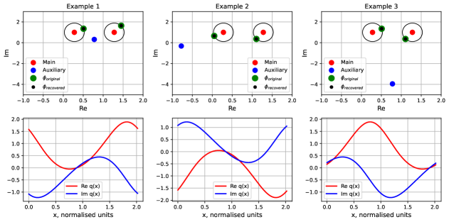
Figure 1. Three examples in the case with $N=1$ with common main spectrum $z_{0}=0.2780+i$ and $z_{1}=1.2780+i$ and different phases $\phi_{0}$ and $\phi_{1}$. The phases are depicted as points $e^{\phi_{j}}$ on the unit circles around the corresponding $z_{j}$.

6.2. Case of $N=2$

In order to provide an example, where $R(z)$ has poles that have to be considered in the phase reconstruction algorithm, we choose a case with $N=2$.

Let $z_{0}=-1+3i$, $z_{1}=5i$, $z_{2}=1+3i$. Ref. [32] shows that the associated $q(x,t)$ is periodic in $x$.

Let $\phi_{0}=0.1$, $\phi_{1}=0.2$ and $\phi_{2}=0.3$. Then the calculated auxiliary spectrum consists of two points, $\mu_{1}=-2.1061+0.4161i$ and $\mu_{2}=2.1061+0.4161i$, and $F(z)=z^{3}-38.4617z$.

In this case, both $\mu_{1}$ and $\mu_{2}$ turn to be the poles of $R(z)$ and thus, we have to proceed using (100) for calculating $J_{00}(z)$. Then, the reconstruction gives $\phi_{0}=0.1007$, $\phi_{1}=0.2000$ and ${\phi_{2}=0.2993}$, which is in good agreement with the original phases. The respective results are depicted in Fig. 2. All data and codes are available on [33].

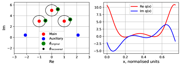
Figure 2. The example in the case with $N=2$ with main spectrum $z_{0}=-1+3i$, $z_{1}=5i$, $z_{2}=1+3i$ and phases $\phi_{0}$, $\phi_{1}$, $\phi_{2}$.

7. Conclusion

A finite-band (finite-genus) solution of the nonlinear Schrödinger equation (in particular, its focusing version) can be characterized in terms of the solution of a Riemann–Hilbert problem specified by (i) the set of endpoints of arcs constituting the contour for the RH problem and (ii) the set of real constants (phases), each being associated with a particular arc. In the present paper we address the problem that can be described as “an inverse problem to the inverse problem”, namely, given the finite-band solution, generated via the solution of the RH problem and specified by a particular set of phases (assuming that the contour endpoints are fixed and that they are such that the finite-band solution is periodic in $x$) and evaluated as a function of $x$ for some fixed $t$, retrieve the phases. Our approach is based on a sequence of consecutive transformations of the RH problem characterizing the solution of the Cauchy problem for the NLS equation in the periodic setting. Particularly, the role of the auxiliary spectrum points in the RH formalism is clarified.

Acknowledgments S. Bogdanov and J. E. Prilepsky acknowledge the support from Leverhulme Trust, Grant No. RP-2018-063.

References

- [1] Gardner CS, Greene JM, Kruskal MD, Miura RM. 1967 Method for solving the Korteweg-de Vries equation. Physical Review Letters 19, 1095–1097.
- [2] Zakharov VE, Shabat AB. 1972 Exact theory of two-dimensional self-focusing and one-dimensional self-modulation of waves in nonlinear media. Journal of Experimental and Theoretical Physics 34, 62–69.
- [3] Ablowitz MJ, Kaup DJ, Newell AC, Segur H. 1974 The inverse scattering transform-Fourier analysis for nonlinear problems. Studies in Applied Mathematics 53, 249–315.
- [4] Ablowitz MJ, Ablowitz M, Clarkson PA. 1991 Solitons, nonlinear evolution equations and inverse scattering vol. 149. Cambridge University Press.
- [5] Novikov S, Manakov SV, Pitaevskii LP, Zakharov VE. 1984 Theory of solitons: the inverse scattering method. Springer Science & Business Media.
- [6] Trogdon T, Olver S. 2015 Riemann–Hilbert problems, their numerical solution, and the computation of nonlinear special functions. Philadelphia, PA: Society for Industrial and Applied Mathematics.
- [7] Fokas AS. 1997 A unified transform method for solving linear and certain nonlinear PDEs. Proceedings of the Royal Society of London. Series A: Mathematical, Physical and Engineering Sciences 453, 61411–1443.
- [8] Fokas AS. 2008 A unified approach to boundary value problems. Society for Industrial and Applied Mathematics.
- [9] Deconinck B, Fokas A, Lenells J. 2021 The implementation of the unified transform to the nonlinear Schrödinger equation with periodic initial conditions. Letters in Mathematical Physics 111, 1–18.
- [10] Fokas A, Lenells J. 2021 A new approach to integrable evolution equations on the circle. Proceedings of the Royal Society A 477, 20200605.
- [11] Turitsyn SK, Prilepsky JE, Le ST, Wahls S, Frumin LL, Kamalian M, Derevyanko SA. 2017 Nonlinear Fourier transform for optical data processing and transmission: advances and perspectives. Optica 4, 307–322.
- [12] Essiambre RJ, Kramer G, Winzer PJ, Foschini GJ, Goebel B. 2010 Capacity limits of optical fiber networks. Journal of Lightwave Technology 28, 662–701.
- [13] Yousefi MI, Kschischang FR. 2014 Information transmission using the nonlinear Fourier transform, Parts I–III. IEEE Transactions on Information Theory 60, 4312–4369.
- [14] Derevyanko SA, Prilepsky JE, Turitsyn SK. 2016 Capacity estimates for optical transmission based on the nonlinear Fourier transform. Nature Communications 7, 12710.
- [15] Goossens JW, Hafermann H, Jaouën Y. 2020 Data transmission based on exact inverse periodic nonlinear Fourier transform, Part I: Theory. Journal of Lightwave Technology 38, 6499–6519.
- [16] Kamalian M, Prilepsky JE, Le ST, Turitsyn SK. 2016a Periodic nonlinear Fourier transform for fiber-optic communications, Part I: theory and numerical methods. Optics Express 24, 18353–18369.
- [17] Kamalian M, Prilepsky JE, Le ST, Turitsyn SK. 2016b Periodic nonlinear Fourier transform for fiber-optic communications, Part II: eigenvalue communication. Optics Express 24, 18370–18381.
- [18] Kamalian M, Vasylchenkova A, Shepelsky D, Prilepsky JE, Turitsyn SK. 2018 Signal modulation and processing in nonlinear fibre channels by employing the Riemann–Hilbert problem. Journal of Lightwave Technology 36, 5714–5727.
- [19] Kamalian-Kopae M, Vasylchenkova A, Shepelsky D, Prilepsky JE, Turitsyn SK. 2020 Full-spectrum periodic nonlinear Fourier transform optical communication through solving the Riemann-Hilbert problem. Journal of Lightwave Technology 38, 3602–3615.
- [20] Goossens JW, Jaouën Y, Hafermann H. 2019 Experimental demonstration of data transmission based on the exact inverse periodic nonlinear Fourier transform. In Optical Fiber Communication Conference pp. M1I–6. Optica Publishing Group.
- [21] Le ST, Prilepsky JE, Turitsyn SK. 2015 Nonlinear inverse synthesis technique for optical links with lumped amplification. Optics Express 23, 8317–8328.
- [22] Belokolos ED, Bobenko AI, Enolskii VZ, Its AR, Matveev VB. 1994 Algebro-geometric approach to nonlinear integrable equations vol. 550. Springer.
- [23] Kotlyarov V, Shepelsky D. 2017 Planar unimodular Baker-Akhiezer function for the nonlinear Schrödinger equation. Annals of Mathematical Sciences and Applications 2, 343–384.
- [24] Bogdanov S, Shepelsky D, Vasylchenkova A, Sedov E, Freire PJ, Turitsyn SK, Prilepsky JE. 2023 Phase computation for the finite-genus solutions to the focusing nonlinear Schrödinger equation using convolutional neural networks. Communications in Nonlinear Science and Numerical Simulation 125, 107311.
- [25] Deift P, Venakides S, Zhou X. 1994 The collisionless shock region for the long-time behavior of solutions of the KdV equation. Communications on Pure and Applied Mathematics 47, 199–206.
- [26] Deift P, Venakides S, Zhou X. 1998 An extension of the steepest descent method for Riemann-Hilbert problems: The small dispersion limit of the Korteweg-de Vries (KdV) equation. Proc. Natl. Acad. Sci. USA 95, 450–454.
- [27] Fokas AS, Its AR. 2004 The nonlinear Schrödinger equation on the interval. Journal of Physics A: Mathematical and General 37, 6091–6114.
- [28] Fokas A, Its AR, Sung L-Y. 2005 The nonlinear Schrödinger equation on the half-line. Nonlinearity 18, 1771.
- [29] Wahls S, Poor HV. 2015 Fast numerical nonnlinear Fourier transforms. IEEE Transactions on Information Theory 61, 6957–6974.
- [30] Olver S. 2012 A general framework for solving Riemann–Hilbert problems numerically. Numerische Mathematik 122, 305–340.
- [31] Olver S. 2019 A Julia package for solving Riemann–Hilbert problems. https://github.com/JuliaHolomorphic/RiemannHilbert.jl.
- [32] Smirnov AO. 2013 Periodic two-phase “rogue waves”. Mathematical Notes 94, 897–907.
- [33] https://github.com/Stepan0001/RHP-Direct-problem.git.