Dynamical Mean Field Theory of the Bilayer Hubbard Model with Inchworm Monte Carlo

Abstract

Dynamical mean-field theory allows access to the physics of strongly correlated materials with nontrivial orbital structure, but relies on the ability to solve auxiliary multi-orbital impurity problems. The most successful approaches to date for solving these impurity problems are the various continuous time quantum Monte Carlo algorithms. Here, we consider perhaps the simplest realization of multi-orbital physics: the bilayer Hubbard model on an infinite-coordination Bethe lattice. Despite its simplicity, the majority of this model’s phase diagram cannot be predicted by using traditional Monte Carlo methods. We show that these limitations can be largely circumvented by recently introduced Inchworm Monte Carlo techniques. We then explore the model’s phase diagram at a variety of interaction strengths, temperatures and filling ratios.

I Introduction

In strongly correlated materials quantum many-body physics shapes the electronic properties. Such materials exhibit a wide variety of unique and interesting phases and transitions [1]. Many of these behaviors are thought to be beyond the predictive power of standard simulation schemes like the density functional theory, where electronic correlation is essentially treated as a static mean field. Embedding methods like the dynamical mean field theory (DMFT) [2]—which contains strong, but local, correlations—have therefore emerged. For model systems, DMFT becomes exact in certain infinite coordination number limits [3]. It can also be used to introduce approximate strong correlation physics into ab initio calculations made by, e.g., density functional theory [4].

DMFT can be phrased as a mapping between an extended model with many-body interactions between orbitals in each unit cell; and a quantum impurity problem representing the correlated orbitals in one unit cell, coupled to an effective noninteracting bath that represents the rest of the system. The coupling density between the impurity and bath, and the connection between the impurity self-energy and the lattice self-energy, are determined by a self-consistency condition [2]. This means that to solve systems with multiple orbitals in each unit cell, a method for solving multiorbital quantum impurity problems is required. In this context, “solving” refers to the calculation of Green’s functions.

While several alternatives exist, the methods most often employed by DMFT practitioners for general multiorbital problems are known collectively as continuous-time quantum Monte Carlo (CT-QMC) algorithms [5]. These methods take perturbative diagrammatic expansions and sum them to very high orders by Monte Carlo integration over diagrams, with most calculations performed in imaginary time on the Matsubara contour. Several different methods exist, based on different expansions and with different regimes of applicability; when these methods do break down, the breakdown typically takes the form of a “sign problem” [6], such that the calculation becomes exponentially harder with decreasing control parameter. For example, the interaction expansion (CT-INT) [7] and auxiliary field (CT-AUX) [8] methods develop sign problems away from half-filling. The hybridization expansion (CT-HYB) [9, 10] can work better in the presence of large, complicated interactions [11], but often develops sign problems when the hybridization in the impurity model has large off-diagonal components. More recently, we proposed an inchworm Monte Carlo method[12] based on the hybridization expansion, which can circumvent some of the sign problems afflicting multiorbital DMFT calculations [13].

One of the earliest models used to investigate multiorbital physics within the framework of DMFT is the bilayer Hubbard model on the infinite dimensional Bethe lattice [14], which we present in detail in Sec. II.1 below. While originally introduced to study the relationship between short-ranged spin correlations and the Mott metal–insulator transition, the model has reemerged over the years: for example, more realistic variations on the model have been used to simulate the metal insulator transition in vanadium dioxide [15, 16, 17]. A two-dimensional version on a square lattice has been considered as a toy model for unconventional superconductivity [18] and realized experimentally using ultracold atoms in an optical lattice [19]. Finally, extensions to hexagonal lattices are currently of great interest in the study of layered 2D materials [20].

The infinite-dimensional bilayer Hubbard model on the Bethe lattice is exactly solvable within DMFT, given an exact solution for the corresponding two-orbital impurity problem. Its phase diagram at half-filling, which includes a Mott metal–insulator transition and an antiferromagnetic regime, was investigated first by Hirsch–Fye Monte Carlo[21] and shortly after by CT-INT [22]. Notably, the 2D model on a square lattice, where DMFT is only approximate, was also probed using an extension of DMFT with a discrete approximation for the bath [23], and by a variational Monte Carlo technique [24]. The paramagnetic regime of the doped system was recently investigated using CT-HYB [25], by taking advantage of a specialized symmetry property to remove the diagonal hybridizations; this suggested the existence of an interesting pseudogap phase at intermediate doping.

Here, we show that the inchworm Monte Carlo method can be used as an impurity solver for the bilayer Hubbard model within DMFT. The robustness of the inchworm scheme to sign problems allows us to extend the phase diagram beyond half-filling without any particular symmetry restrictions, enabling exploration of ferromagnetic and antiferromagnetic response. We use this to investigate the effect of doping on the metallic and magnetic properties of the system, and analyze the results to reveal simple short-ranged mechanisms behind much of the phenomenology. The rest of this work is structured as follows: Sec. II briefly describes the model (II.1) and methodology (II.2). In Sec. III we first compare the CT-HYB impurity solver with its inchworm counterpart (III.1). We then show how we determine phase transitions from our numerical data (III.2), and finally present and discuss the phase diagram (III.3). In Sec. IV we conclude and discuss future prospects.

II Theory

II.1 Model

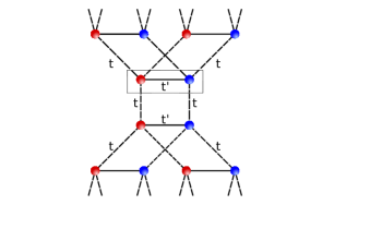
Figure 1: Illustration: a small region in the bilayer Hubbard model on a Bethe lattice with $Z=3$ (we consider the limit $Z\rightarrow\infty$). Blue and red spheres, respectively, represent orbitals in the first and second layer. Orbitals on adjacent sites within a layer are coupled by hopping amplitudes $t$. Within each dimer or unit cell, one of which is marked by a rectangular box, particles can hop between layers with hopping amplitude.

We define the bilayer Hubbard model on the Bethe lattice in the infinite coordination number limit $Z\rightarrow\infty$. In Fig. 1 we provide an illustration with $Z=3$. The model comprises two identical Hubbard models, or layers, on Bethe lattices with hopping $t$, chemical potential $\mu$ and interaction strength $U$. Each site in the first layer is coupled to its counterpart in the second with hopping $t^{\prime}$. The Hamiltonian is given by:

$$H =-t\sum_{\left\langle ij\right\rangle\sigma}\left(a_{i\sigma}^{\dagger}a_{j\sigma}+b_{i\sigma}^{\dagger}b_{j\sigma}\right)+t^{\prime}\sum_{i\sigma}\left(a_{i\sigma}^{\dagger}b_{i\sigma}+b_{i\sigma}^{\dagger}a_{i\sigma}\right)$$

$$-\sum_{i\sigma}\mu\left(n_{i\sigma}^{\left[a\right]}+n_{i\sigma}^{\left[b\right]}\right)+U\sum_{i}\left(n_{i\uparrow}^{a}n_{i\downarrow}^{a}+n_{i\uparrow}^{b}n_{i\downarrow}^{b}\right).$$ (1)

The subscript $\sigma\in\left\{\uparrow,\downarrow\right\}$ denotes spin, and $a^{\dagger}$($b^{\dagger}$) creates an electron in layer $a$($b$). In the second line, $n_{i\sigma}^{a}\equiv a_{i\sigma}^{\dagger}a_{i\sigma}$ and $n_{i\sigma}^{b}\equiv b_{i\sigma}^{\dagger}b_{i\sigma}$. We also define the ratio between the inter-layer and intra-layer hopping, $\alpha\equiv t^{\prime}/t$. To obtain a nontrivial infinite coordination number limit, we rescale $t$ to $\frac{t}{\sqrt{Z-1}}$, then set this to $1$ to define our unit of energy. This scaling is not applied to $t^{\prime}$.

II.2 Methodology

The DMFT method provides a self consistent mapping from Eq. (1) onto a quantum impurity model [2]. In the present model and for antiferromagnetic order, the self consistency requirement takes on a particularly simple form [14, 22]:

$$\mathcal{\boldsymbol{G}}_{\sigma}^{-1}\left(i\omega_{n}\right) \equiv\int_{0}^{\beta}\mathrm{d}\tau e^{i\omega_{n}\tau}\mathcal{\boldsymbol{G}}_{\sigma}^{-1}\left(\tau\right)$$ (2)

$$=\left(\begin{array}[]{cc}i\omega_{n}+\mu&-\alpha t\\ -\alpha t&i\omega_{n}+\mu\end{array}\right)-\boldsymbol{\Delta}_{\sigma}\left(i\omega_{n}\right),$$

where $\mathcal{\boldsymbol{G}}_{\sigma}\left(i\omega_{n}\right)$ is the Weiss field at Matsubara frequency $\omega_{n}$. Here the hybridization function,

$$\boldsymbol{\Delta}_{\sigma}=t^{2}\boldsymbol{G}_{-\sigma}\left(i\omega_{n}\right),$$ (3)

is obtained from the local Green’s function at the (arbitrarily chosen) site $i=0$, such that $a_{\sigma}=a_{0\sigma}$ and $b_{\sigma}=b_{0\sigma}$:

$$\boldsymbol{G}_{\sigma}\left(\tau\right)\equiv-\left(\begin{array}[]{cc}\left\langle\mathrm{T}_{\tau}a_{\sigma}\left(\tau\right)a_{\sigma}^{\dagger}\left(0\right)\right\rangle&\left\langle\mathrm{T}_{\tau}a_{\sigma}\left(\tau\right)b_{\sigma}^{\dagger}\left(0\right)\right\rangle\\ \left\langle\mathrm{T}_{\tau}b_{\sigma}\left(\tau\right)a_{\sigma}^{\dagger}\left(0\right)\right\rangle&\left\langle\mathrm{T}_{\tau}b_{\sigma}\left(\tau\right)b_{\sigma}^{\dagger}\left(0\right)\right\rangle\end{array}\right).$$ (4)

Note that this assumes the spins in adjacent sites can be flipped by antiferromagnetism, forming a bipartite lattice. A small symmetry breaking term was also applied to the Hamiltonian in the initial DMFT iteration when seeking antiferromagnetic solutions.

The impurity model to be solved is then defined by the effective action

$$S_{\mathrm{eff}} =-\sum_{\sigma}\int_{0}^{\beta}\mathrm{d}\tau\mathrm{d}\tau^{\prime}\mathrm{d}\tau^{\prime}\mathbf{c}^{\dagger}\left(\tau\right)\cdot\boldsymbol{\mathcal{G}}_{\sigma}^{-1}\left(\tau-\tau^{\prime}\right)\cdot\mathbf{c}\left(\tau^{\prime}\right)$$ (5)

$$+U\int_{0}^{\beta}\mathrm{d}\tau\left(n_{\uparrow}^{a}\left(\tau\right)n_{\downarrow}^{a}\left(\tau\right)+n_{\uparrow}^{b}\left(\tau\right)n_{\downarrow}^{b}\left(\tau\right)\right),$$

where $\mathbf{c}^{\dagger}\left(\tau\right)\equiv\left(a^{\dagger}\left(\tau\right),b^{\dagger}\left(\tau\right)\right)$, $n_{\sigma}^{a}\left(\tau\right)\equiv a_{\sigma}^{\dagger}\left(\tau\right)a_{\sigma}\left(\tau\right)$ and $n_{\sigma}^{b}\left(\tau\right)\equiv b_{\sigma}^{\dagger}\left(\tau\right)b_{\sigma}\left(\tau\right)$. This is a two-orbital impurity problem. For this particular problem, at $\mu=-U/2$ the system becomes particle–hole symmetric, and CT-INT works without a sign problem [22]. The off-diagonal elements in Eq. (3) lead to sign problems in CT-HYB, which can be eliminated in the paramagnetic case by transforming to the bonding/antibonding orbital basis, where $\boldsymbol{\Delta}_{\sigma}$ is diagonal. Neither algorithm works robustly in the general case. Here, we employed an inchworm Monte Carlo algorithm based on CT-HYB, but able to deal with the multiorbital sign problem emerging from nondiagonal hybridization functions [13]. At their core, inchworm algorithms are a resummation technique for diagrammatic Monte Carlo methods. They were originally developed almost a decade ago to address the dynamical sign problem for populations dynamics in the real time hybridization expansion[12] and related expansions for the spin–boson model [26, 27, 28, 29, 30, 31], but were soon extended to Green’s functions[32] and used to perform real-time DMFT calculations [33]. In addition to a variety of applications in nonequilibrium physics [34, 35, 36, 37, 38, 39, 40, 41, 42], several extensions and generalizations have been aimed at making these methods more useful as imaginary time impurity solvers [43, 44, 45]. Our present implementation includes several optimizations not present in the previous work [13], including fast diagram summations[46] and a sparse representation of local propagators that takes advantage of conserved quantum numbers. We plan to discuss these technical aspects in detail in future work along with a public release of our code.

We note in passing that recent advances in tensor train methods as a substitute for Monte Carlo techniques can also circumvent sign problems, and may offer an alternative route to solving the impurity problems appearing here [47, 48]. Novel decomposition schemes for finite-order diagrammatic methods are another interesting development in this regard [49].

III Results

III.1 Sign problem in CT-HYB and inchworm algorithm

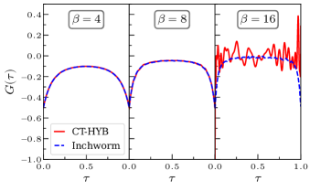
Figure 2: Development of the sign problem in CT-HYB (solid red curves) as temperature is decreased, and comparison to inchworm Monte Carlo (dashed blue curves) at interaction strength $U=4$, $\alpha=1$ and half-filling. The same computation time is used for each of the six simulations shown.

The DMFT algorithm consists of a sequence of iterations, in each of which the impurity solver is used to compute the Green’s function of Eq. (5) for a hybridization function obtained from the previous iteration or—in the first iteration—from the noninteracting problem. In the CT-HYB impurity solver [9], generally a very efficient choice at anything but the smallest interaction strengths [11], sign problems appear when the hybridization function develops large nondiagonal components. To demonstrate this, consider Fig. 2, where the Green’s function is calculated for interaction strength $U=4$ and tunneling amplitude ratio $\alpha=1$, at half-filling. All simulations shown in the figure and in the rest of this subsection, with both methods, were obtained with the same total amount of computer time ($\sim 150$ minutes on 56 CPU cores). We used the implementation of CT-HYB [50] based on the ALPSCore libraries [51]. While CT-HYB (solid red curves) performs well at the higher temperatures $\beta=4$ and $\beta=8$, it breaks down at $\beta=16$. The corresponding data from an inchworm calculation [13] based on the same expansion (dashed blue curves) remains reliable at the entire temperature range shown.

While the example in Fig. 2 is illustrative, it is difficult to ascertain how typical it is without further exploring the parameter space. To facilitate this it is convenient to define a measure of the error, and we choose the jackknife variance over $n=5$ independent realizations of the calculation with different random seeds, averaged over imaginary time:

$$\Delta G\equiv\frac{1}{\beta}\int_{0}^{\beta}\mathrm{d}\tau\frac{1}{n\left(n-1\right)}\sum_{i=1}^{n}\left(G_{i}\left(\tau\right)-\bar{G}\left(\tau\right)\right)^{2}.$$ (6)

In Fig. 3 we plot this measure on a logarithmic scale as a function of $\alpha$, for $U=3$ and two temperatures, still at half-filling. Results from CT-HYB and inchworm are shown in red and blue, respectively; while results at $\beta=16$ and $8$ are shown in solid and dashed curves, respectively. Once again, every data point uses the same overall computer time as in Fig. (2). CT-HYB is substantially more accurate at small $\alpha$, i.e. when there is little or no dimerization. However, its accuracy rapidly deteriorates due to a severe sign problem at larger values of $\alpha$, especially at low temperatures. It recovers slightly at very large values of $\alpha$. The inchworm method, while not as accurate at small $\alpha$ near the part of parameter space corresponding to a normal Hubbard model, generally suffers less from both an increase in both $\alpha$ and the lowering of temperature. It becomes very accurate at large $\alpha$, and generally converges more easily when the system is in an insulating state.

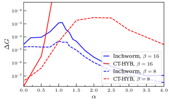
Figure 3: Stochastic error estimates from inchworm (blue curves) and CT-HYB (red curves) as a function of $\alpha$ at two temperatures (solid and dashed curves). The interaction strength is set to $U=3$ and the system is half-filled.

Next, in Fig. (4), we map out the dependence of the sign problem on $\alpha$, $U$ and $\beta$ at half-filling. We carry out calculations of $\Delta G$ as before. The red and blue shaded regions denote parameters where CT-HYB and the inchworm method, respectively, provide a value of $\Delta G$ lower than $10^{-2}$ for the given runtime. Note that this criterion is arbitrary and the results are implementation-dependent; nevertheless, this procedure provides a useful and intuitive description of the limitations of the methods. In the high temperature case $\beta=4$ (left panel), both methods converge for the entire parameter regime. At $\beta=8$ (middle panel), a region forms at $1<\alpha<3$ and $U<4$ where the performance of CT-HYB degrades, but the inchworm method continues to work well. As we go even lower in temperature to $\beta=16$ (right panel), CT-HYB fails for $\alpha\gtrsim 0.5$ except at large $U$. Here a parameter region where inchworm begins to fail as well (white region) is also visible. This appears at small $U$ and around $\alpha=1$; note that this behavior is also seen in Fig. 3, where the highest peak in $\Delta G$ for the inchworm method appears near $\alpha=1$. While the errors in CT-HYB at these parameters make most of the parameter space completely intractable at $\beta=16$, inchworm data could still be obtained here given a reasonable investment in computational resources. We expect that if it becomes necessary to perform simulations at much lower temperatures, further algorithmic improvements will be required even for the inchworm method.

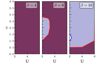
Figure 4: Parameter regions where methods converge easily, as a function of $U$ and $\alpha$. The red and blue shaded regions show where the CT-HYB and inchworm methods, respectively, achieved errors $\Delta G$ below a threshold value of $10^{-2}$ for a given amount of computational resources. Panels show different temperatures, decreasing from left to right.

III.2 Studying phase transitions

We will be interested in two types of order parameter. The first distinguishes between paramagnetic (PM) and antiferromagnetic (AFM) states, and the second between metallic and insulating ones. These are the same distinctions made in previous work [22], where the entire phase diagram at half filling was obtained for $0\leq U\leq 5$ at $\beta=10$ using CT-INT as the impurity solver. As we noted, CT-INT has no sign problem at half filling, and converges rapidly at weak interaction strengths. It is therefore an ideal choice for this problem, and can serve as an excellent benchmark for the hybridization-expansion-based inchworm method.

We will first discuss the PM/AFM transition. One interesting finding in Ref. [22] was that at the limit of low temperature and large interaction strength $U$, the system undergoes a transition from AFM to PM as $\alpha$ increases past $\sqrt{2}$. It was suggested that this is due to the transition happening when the effective intra-layer Heisenberg exchange coupling, $J^{\prime}\sim\frac{t^{\prime 2}}{U}$, is twice the size of its inter-layer counterpart $J\sim\frac{t^{2}}{U}$. This, because every dimer has one $J^{\prime}$ coupling and two $J$ couplings. This low energy argument is correct at low temperatures, but can be expected to break down at higher ones. In particular, for larger values of $U$ we might expect this breakdown to occur when the temperature is comparable to the larger of $J^{\prime}$ and $J$.

In Fig. 5 we plot the zero-field magnetization predicted from our inchworm-based DMFT calculations at $\beta=10$ and half filling, for a range of $U$ values. This is defined simply as

$$M=\left\langle n_{\uparrow}^{a}+n_{\downarrow}^{b}-n_{\downarrow}^{a}-n_{\uparrow}^{b}\right\rangle,$$ (7)

and—being a static property—can be directly obtained from inchworm Monte Carlo calculations [12]. In practice, we apply a small staggered magnetic field during the first DMFT iteration in order to break symmetry; then we turn it off, and allow the DMFT self-consistency to evolve to either a symmetry-broken ($M\neq 0$) or symmetric $\left(M=0\right)$ state. In practice, our numerical criterion for this was that the zero field magnetization, Eq. (7), be over an arbitrary threshold value, $M_{\mathrm{threshold}}\equiv 0.03$.

The $U=4$ result is consistent with results from Ref. [22], where similar data is shown. The phase transition indeed occurs at $\alpha\approx\sqrt{2}$, as expected from the low energy theory. We also present a sequence of curves at higher values of $U$, still at the same temperature. It is clear that the value of $\alpha$ at which the transition occurs at this temperature decreases with $U$. At $\alpha=0$ the system is a normal Hubbard model, and the decrease in magnetization at larger values of $U$ is related to the known decrease in the Curie temperature, which is expected to shift inversely with $U$ [52, 53, 54]. At large values of $U\gtrsim 6$, magnetization increases with $\alpha$ before decreasing again, showing that an intermediate inter-layer coupling can either suppress or enhance magnetic properties.

.

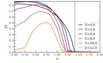
Figure 5: Zero-field magnetization at $\beta=10$ and various values of $U$, plotted as a function of $\alpha$. The theoretical low temperature limit for the AFM–PM transition [22] is shown as a vertical dashed line at $\alpha=\sqrt{2}$. The line widths indicate a confidence interval given by the absolute value of the difference between the last two DMFT iterations.

The second order parameter we will discuss is an approximation for the spectral function at the chemical potential, and therefore a proxy for metallicity:

$$A\left(\omega=\mu\right)\simeq-\frac{\beta}{\pi}G\left(\tau=\beta/2\right).$$ (8)

The approximation becomes increasingly accurate at the low temperature limit $\beta\rightarrow\infty$, but is commonly used in the DMFT literature at finite temperature [2]. One possible alternative is to perform analytical continuation and define the transition according to the formation of a gap, but this requires additional assumptions. A more rigorous, but challenging, route is to solve the problem on the real axis using nonequilibrium dynamical mean field theory [55, 56, 57, 58, 42]; we will explore this in future work. Here, we chose to define a simple, but arbitrary, transition threshold. When $-\frac{\beta}{\pi}G\left(\tau=\beta/2\right)<0.25$, we refer to the system as insulating; otherwise, we refer to is as metallic. This definition should be seen as qualitative.

Fig. 6 shows how this definition can be used to investigate the metal–insulator transition that occurs when the system is doped. The metallic order parameter from Eq. (8) is shown as a function of the chemical potential, at two values of the interaction strength $U$ and two values of the hopping ratio $\alpha$. In all cases, higher doping takes the system from the insulating to the metallic regime. Increasing both $U$ and $\alpha$ drives the transition to higher chemical potentials. When $U=2.5$ and $\alpha=1$, we can observe a drop in the order parameter at larger chemical potentials and an eventual reentrance into insulating behavior due to the reduction of free charge carriers. The latter will happen at high enough chemical potential shift for all parameters.

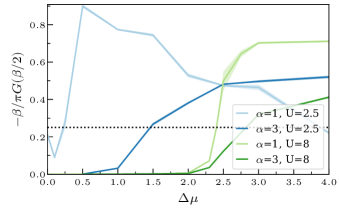
Figure 6: Proxy for metallic behavior as a function of the chemical potential shift $\Delta\mu$, at inverse temperature $\beta=16$. The dotted horizontal black line denotes the (arbitrarily chosen) threshold value we use to indicate the transition from an insulating to a metallic state. The line widths indicate a confidence interval given by the absolute value of the difference between the last two DMFT iterations.

III.3 Phase diagram

Using the order parameters and thresholds discussed in III.2, we performed a set of calculations at $U=2.5$ and $U=8$, mapping out the phase diagram of the model at each of these interaction strengths and temperature $\beta=16$ with respect to the ratio $\alpha$ between inter-layer and intra-layer hoppings; and the chemical potential shift from half filling, $\Delta\mu=\mu+\frac{U}{2}$. Due to symmetry considerations, it is sufficient to examine the $\Delta\mu>0$ part of the diagram. The two maps are presented in the left and right panels of Fig. 7. The shaded red region in each denotes parameters where we found the system to be antiferromagnetic. Similarly, the blue region denotes parameters where we predict metallic behavior. Four combinations of order parameters are possible, embodying four distinct phases: the AFM insulator, AFM metal, PM insulator and PM metal.

We begin by considering previously available results. The $\alpha=0$ case (bottom edge of both panels in Fig. 7) corresponds to the normal Hubbard model. The behavior there is consistent with that known in the literature [59]: for $U=2.5$, the system is in the AFM state for $\Delta\mu\lesssim 0.5$. The metallic regime begins when $\Delta\mu\approx 0.2$ and ends at $\Delta\mu\approx 0.5$. At $U=8$, the AFM regime expands while the insulating regime shifts to larger values of $\Delta\mu$.

Next, we consider the $\Delta\mu=0$ case (left edge of both panels in Fig. 7), which was explored by Hafermann et al. in Ref. [22]. At $U=2.5$, the system is an AFM Mott insulator at $\alpha=0$. Increasing $\alpha$ drives it first to an AFM metallic phase, then to a PM band insulator state. Depending on the thresholds and temperature, a small PM metallic region may exist at $\alpha\approx 1.7$ [22]. At $U=8$, however, the system goes directly from an AFM insulator to a band insulator at $\alpha\approx\sqrt{2}$; this behavior was also found in Ref. [22] at $U\apprge 4$. Note also the difference from the behavior in Fig. 5, where $\beta=10$.

The rest of the phase diagram (everywhere else in the two panels of Fig. 7, where neither $\alpha=0$ nor $\Delta\mu=0$) is where both DMFT calculations based on the standard CT-HYB, CT-INT or CT-AUX methods face sign problems unless special symmetries can be taken advantage of, as in Refs. [16, 17]. Our CT-HYB-based inchworm method works well in the entire parameter space, without any need for symmetrization, and can be used to obtain both the metallic and AFM order parameters. For both values of $U$, an AFM regime appears at small $\alpha$ and $\Delta\mu$. Increasing $U$ extends this regime in $\Delta\mu$, while simultaneously contracting it in $\alpha$. The metallic behavior appears at intermediate values of $\Delta\mu$ and is shifted approximately linearly in $\alpha$. The metallic region always appears to be simply connected. In particular, at small $U$ the AFM metallic state on the $\Delta\mu=0$ line is connected to its counterpart on the $\alpha=0$ line. As a result of this, at small $U$ the metallic and AFM regimes overlap in a narrow band surrounding the AFM insulator at the origin, but this overlap shrinks with increasing $U$ as the metallic phase recedes from the $\Delta\mu=0$ line.

We emphasize that the particular size and shape of the regions and overlaps depends to some degree on our choice of order parameters and thresholds, but we expect the general physical trends to be robust.

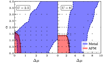
Figure 7: Phase diagram of the bilayer Hubbard model at $\beta=16$ as function of the ratio between the hopping terms $\alpha=t^{\prime}/t$ and the doping $\Delta\mu$. The left and the right panel has coulomb onsite interaction $U$ of $2.5$ and $8$, respectively. Dots indicate parameter combinations where a calculation was made, and bilinear interpolation is used to construct the curves as described in III.2.

Much of the dependence of physical behavior on doping can stem from local mechanisms like energetics and population switching effects within a unit cell. It can therefore be understood to some degree by considering a substantially simplified model: two adjacent dimers (here a dimer refers to two coupled orbitals, one of which is in each layer). This model contains only four spin-half orbitals, and can easily be solve by exact diagonalization (ED); it also becomes equivalent to the lattice model at the fully dimerized limit $\alpha\rightarrow\infty$, and bears some resemblance to a DMFT calculation with a minimal discrete bath, at least with paramagnetic boundary conditions. Since no spontaneous symmetry breaking can occur in the ED solution without a self-consistency condition, we solve the system in the presence of a small staggered field $h=0.1$ that induces an AFM state. In Fig. 8 we present a detailed view of how several local observables depend on the chemical potential, for $U=2.5$ and $U=8$ (red and blue curves, respectively); and for the numerically exact solution on Bethe lattice and the two-dimer model (solid and dashed lines, respectively).

The top row of Fig. 8 shows the mean occupancy of the orbitals within a unit cell. At $\Delta\mu=0$ the system is half filled: there are, on average, two electrons per unit cell. Naturally, the occupancy rises as the chemical potential increases, and at $\Delta\mu=10$ the system becomes completely filled (4 electrons per unit cell) at all the parameter sets shown here. In the lattice model, the increase in occupation is continuous and mostly linear. In the two-dimer model, it increases in a series of steps with a width set by the temperature, but over a similar range of chemical potentials.

The second row of Fig. 8 shows the AFM order parameter $M$. It is clear that as the occupation increases, magnetic behavior is suppressed. This is not surprising when considering that the half-occupied local state $\left|\uparrow\right\rangle_{a}\left|\downarrow\right\rangle_{b}$ has the maximal AFM response. In the two-dimer model, the drop in magnetism is associated with the first jump in population. However, it is clear that the two-dimer model does not fully capture the physics of the AFM–PM transition, even with the addition of a symmetry-breaking field.

We now consider the metal–insulator transition, which is captured by the order parameter of Eq. (8). This is plotted in the third row of Fig. 8. While the two-dimer always produces sharp peaks in the proxy for the density of states, these peaks do appear in the approximate region where the broadened density of states appears in the lattice model. This region appears when the system begins to exit the half-occupied state, which characterizes a Mott insulator; and disappears when it enters the fully-occupied state, which characterizes a band insulator.

Finally, the bottom row of Fig. 8 shows the probability of occupying metal-like local states with 3 electrons. In the lattice model, this probability appears and disappears in tandem with the presence of a metallic order parameter. In the two-dimer model, the association between these observables is still apparent, especially at larger values of $\alpha$; but both the magnitude and extent in chemical potential where this state is likely are significantly underestimated. The large discrepancy between the two-dimer and lattice models in all panels on the bottom row of Fig. 8 illustrates the fact that metallic behavior, in particular where it is associated with Kondo correlations, is where the analogy between these two models breaks down most noticeably.

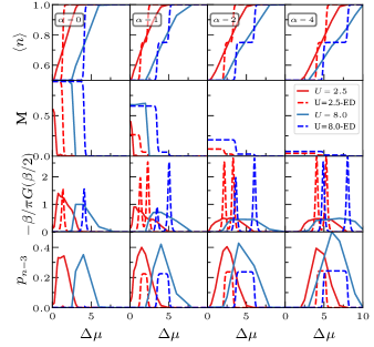
Figure 8: The average occupation (top row), staggered magnetization (second row), metallic order parameter (third row), and probability of occupying states with $3$ electrons in the unit cell (bottom row); all as a function of the chemical potential shift $\Delta\mu$, for two values of the coulomb interaction (red and blue curves) and for four values of the ratio $\alpha$ between inter-band and intra-band hopping amplitudes (in different columns). Solid lines denote the full DMFT solution on the Bethe lattice with inchworm Monte Carlo as the impurity solver. Dashed lines are ED calculations for the two-dimer model (see text).

IV Conclusions

We presented a study of the infinite-dimensional bilayer Hubbard model on the Bethe lattice. The dynamical mean field approximation is exact for this model, given a procedure for solving the associated multiorbital quantum impurity model. We showed that the inchworm quantum Monte Carlo method enables this solution in parameter regimes where other methods fail due to severe sign problems. This allowed us to obtain the model’s phase diagram outside of half-filling.

Our results show that at combinations of temperature and interaction strength where the half-filled model has a metallic regime, it merges with the corresponding metallic regime in the normal Hubbard model, where the two layers are isolated from each other. It can then overlap with the antiferromagnetic regime that exists near half-filling and at weak inter-layer coupling. At stronger interaction strengths the metallic regime is pushed towards higher chemical potentials. We also showed that most, though not all, of the qualitative properties of the phase diagram can be understood from the local energetics and state population probabilities within a unit cell.

In addition to shedding light on the properties of the doped bilayer Hubbard model, our work illustrates some of the limitations of standard quantum Monte Carlo methods in the study of multiorbital strongly correlated electron physics. It then highlights inchworm techniques as a way around such limitations, showing that they enable access to parameter regimes that were previously difficult to simulate. We expect the methodology introduced here may be useful for many other situations where sign problems have limited our ability to answer important scientific questions regarding complex quantum materials.