Maximal Elements of Quantum Communication
Abstract.
A prepare-and-measure scenario is naturally described by a communication matrix which collects all conditional outcome probabilities of the scenario into a row-stochastic matrix. The set of all possible communication matrices is partially ordered via the ultraweak matrix majorization relation. By considering maximal elements in this preorder for a subset of matrices implementable in a given theory, it becomes possible to identify communication matrices of maximum utility, i.e., matrices that are not majorized by any other matrices in the theory. The identity matrix of an appropriate size is the greatest element in classical theories, while the maximal elements in quantum theory have remain unknown. We completely characterize the maximal elements in quantum theory. In particular, we show that the identity matrix is the only maximal element in quantum theory but, as opposed to a classical theory, it is not the greatest element. Quantum theory can hence be seen to be distinct from classical theory by the existence of incompatible communication matrices.
1. Introduction
One of the fundamental pursuits in quantum information science is to identify and investigate different kinds of communication scenarios, with the aim of finding differences to classical communication. Notable examples are super dense coding [1], quantum teleportation [2] and quantum key distribution [3]. Communication scenarios such as these are not only important in the study of entanglement and quantum theory in general, but they also pave the way for new applications in the field of quantum computation and cryptography.
Recently, there has been new findings where a communication advantage for quantum systems has been demonstrated. A quantum advantage is often shown in a setting where the communicating parties share entanglement [4, 5] or shared randomness [6, 7, 8] as a resource. However, a quantum advantage can also be demonstrated in other settings [9, 10, 11, 12, 13] and without any extra resources [14, 15, 16, 17]. Demonstrations such as these are of crucial importance, as it is not clear in which scenarios exactly are quantum systems better than their classical analogues. The same problem arises in quantum computation, too; while some algorithms are known which perform exponentially faster than existing algorithms on a classical computer, such as Shor’s algorithm [18], it is not known exactly for which computational problems an exponential speed-up is possible or if this speed-up is theoretically robust. In fact, a kind of tug-of-war competition seems to be going on between classical and quantum computing –- often when significant advances are made in quantum computing, classical computers are quick to catch up any lost ground on computing time [19, 20].
In this article we take a slightly different approach to previous works on the topic. We focus on the one-way communication scenario between two parties (Alice and Bob), where Alice prepares a classical or quantum system and sends it to Bob, who then performs a measurement on the state of the system. We assume that Alice and Bob do not share any extra resources such as shared randomness or entanglement. Instead of presenting a single communication scenario displaying a quantum advantage, we will give a complete and exhaustive mathematical characterization on one-way communication devices of “maximum utility” in the quantum case. In order to present our results, we are going to expand on the theory of ultraweak matrix majorization [21, 22], which gives a physically motivated preorder in the set of communication matrices. Our results bring new intuitive understanding both mathematically and physically. In particular, our main result sheds new light into the differences between classical and quantum communication devices.
The rest of the article is organized as follows. In Sections 2 and 3 we give a brief introduction to the theory of communication matrices and ultraweak matrix majorization. Section 4 analyzes ultraweak matrix majorization from the point of view of some physically motivated actions, and presents a novel result that is used in the main theorem. Finally, in Section 5 we give a complete characterization on which quantum communication devices are maximal in the preorder defined by the ultraweak matrix majorization. We close the article in Section 6 by discussing the physical significance of our results.
2. Communication tasks
In a one-way communication scenario one party, Alice, attempts to send a message to another party, Bob. Usually the size of the message is taken to be limited. For instance, the message could consist of a fixed number of units of some specified physical communication medium. In the following we are considering an abstract operational description of communication scenarios. In particular, we typically describe the communication medium as a classical -level system or a -level quantum system, i.e., a quantum system associated with -dimensional Hilbert space.
In the operational picture, depicted in Fig. 1, Alice operates a state preparation device with inputs. This means that Alice has in her possession a device capable of preparing states of the communication medium with different labels. Some of the inputs of the device may lead to the same state being outputted. In each round of communication, Alice prepares one state from her device and sends it to Bob. Bob operates a measurement device with outputs. A measurement device is a device that takes as input a state and gives one of its outputs with a probability depending on the input state.
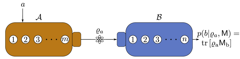
In the quantum setting, we describe Alice’s state preparation device by a finite state ensemble . Each of the states in the state ensemble is a positive operator of unit trace. In general the quantum state space is described by , where is a complex separable Hilbert space, taken to be of finite dimension in this article, and is the set of bounded linear operators acting on .
A quantum mechanical measurement device is described by a normalized positive operator measure, or a POM for short (also called a POVM in the literature). More specifically, a measurement is described by a finite set of effect operators corresponding to different outcomes. The set of effects is defined as . A normalized POM is then a finite collection of effects such that . In this work a POM is always taken to be normalized. Probabilities of different outcomes are given by the Born rule:
| (1) |
where is the conditional probability of observing outcome when performing a measurement of on state . Especially important to us will be POMs whose every effect is a rank-1 operator. Such POMs are simply called rank-1 POMs. A POM is sharp if its every effect is a projection. Rank-1 effects are also sometimes called indecomposable in the literature, as these effects cannot be written as positive linear combinations of other effects [23].
Given a finite state ensemble and a POM with outcomes, we can collect all the conditional outcome probabilities into a row-stochastic matrix:
| (2) |
Such a matrix is called a communication matrix or communication channel, and they arise naturally when considering outcome probabilities in a one-way communication scenario.
In a typical communication scenario, Alice and Bob are trying to accomplish some specific communication task. For instance, Alice and Bob’s goal may be that Bob can unambiguously distinguish which state was sent by Alice, or they may try to minimize the error probability in distinguishing the state, leading to minimum error state discrimination. All communication tasks are hence described by some communication matrix, which defines the desired output probabilities for each state. As an example, communication matrices describing communication tasks of minimum error discrimination of three states with zero error and uniform antidistinguishability [24, 25, 26] of three states are given as follows:
| (3) |
An immediate question that arises when studying communication is which set of communication matrices is implementable in a given physical theory? Implementable here means that there exists a set of states and a measurement that implement the probabilities given by the communication matrix. If we denote a state space by , then the corresponding set of implementable communication matrices of size is denoted by . The set of all such matrices is then . The set of all by row-stochastic matrices is denoted by , or simply for the union of all row-stochastic matrices of finite size.
In the current investigation we focus on two special classes of state spaces. Firstly, we denote by the state space in -dimensional Hilbert space as a short-hand notation for . In main focus will be the set , the set of communication matrices implementable in -dimensional quantum theory via the Born rule defined in Eq. (1). Secondly, we denote a -dimensional classical state space by . A set of communication matrices implementable by a classical -level system is special in the sense that all communication matrices can be seen to be of a particular form [22]. Namely, if , then for some row-stochastic matrices and . For a given communication matrix , the minimum value of for which there exists row-stochastic matrices and such that is called the classical dimension of the matrix . The classical dimension is intimately related to the concept of nonnegative rank [27]. In fact, for communication matrices the two concepts coincide.
Analogously to the classical dimension, the quantum dimension of a communication matrix is defined as the minimum value of for which there exists a state ensemble and a POM with outcomes such that . For an arbitrary communication matrix , the quantum dimension can be seen to be exactly given by the positive semidefinite rank (or psd rank [28, 29]) of .
A second question regarding sets of communication matrices is if some communication matrices are harder to implement than others. As we will see in the next section, this question can be formulated in a precise mathematical way.
3. Ultraweak matrix majorization
Given two communication matrices , we may ask if one of them is harder to implement than the other. Suppose there exist row-stochastic matrices such that . It follows that cannot be any harder to implement than . To see this, suppose has a quantum implementation with some state ensemble and a POM with outcomes. Define new states by and a new POM by . Then we get
That is, the matrix has an implementation by pre- and post-processing the states and measurement outcomes in ’s implementation. The pre- and post-processings are naturally given by the matrices and . Whenever in the above sense, we say that the matrix is ultraweakly majorized by the matrix .
Definition 1.
Let . If there exists row-stochastic matrices and such that , we say that is ultraweakly majorized by and denote . Whenever and we denote and say and are ultraweakly equivalent. Each matrix defines an ultraweak equivalence class given by .
The ultraweak matrix majorization, along with monotone functions characterizing it, have been studied in detail in [21, 22]. It is straightforward to see that the ultraweak matrix majorization is a preorder (i.e. reflexive and transitive) on the set of communication matrices. In the usual way, this preorder determines a partial order in the set of all equivalence classes of communication matrices. We denote by the set of all equivalence classes of matrices in .
We recall the definition of a monotone function for ultraweak matrix majorization and introduce some useful monotones we are going to use. A thorough treatment can be found in [22].
Definition 2.
A function is an ultraweak monotone function if implies for all and in .
Some known ultraweak monotone functions include the following. For all matrices the functions
-
•
-
•
max monotone [30]:
-
•
min monotone [22]:
-
•
distinguishability monotone [22]:
-
•
nonnegative rank [27]:
-
•
positive semidefinite rank [28]:
are ultraweak monotones. We recall that for all we have , and . For we have , and .
As mentioned before, the nonnegative and positive semidefinite ranks correspond to the optimal dimensions of the classical and quantum implementations of the matrix. The regular rank is connected to the linear dimension of the underlying operational theory. is related to the optimal success probability in minimum error discrimination tasks (and the basic decoding theorem [31]), while has an operational interpretation relating to noise. The monotone gives the exact number of distinct code words that are possible to send without error by the devices implementing . In the present article we are going to leverage the monotones , and . The following example demonstrates the usefulness and application of the monotone .
Example 1.
Consider the following communication matrices:
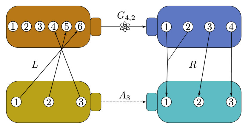
We have , so clearly . However, we see that . Therefore witnesses that , i.e., it is not possible to find such that . The relation is illustrated in Fig. 2.
As we explained earlier, all classical communication matrices belonging to are characterized by being ultraweakly majorized by . Thus the matrix is the unique greatest element in classical -dimensional theory, in the sense that is the greatest element in the partially ordered set of equivalence classes in . Motivated by this we make the following definition.
Definition 3.
Let . We say that is ultraweakly maximal in if implies for all .
We see that the ultraweakly maximal elements in a given theory are the communication matrices of best utility in the sense that there do not exist any communication matrices that are stronger than them. The characterization of all maximal elements of the ultraweak preorder was stated as an open problem in [32]. In the present work we will fully address this problem in the quantum case. Surprisingly, it turns out that quantum and classical theories are similar in that is also the only maximal element in . In order to see this, we will first give additional physical motivation to the ultraweak matrix majorization in the next section.
4. Physically motivated pre- and post-processing actions
For two communication matrices it is straightforward to verify that and are ultraweakly equivalent in the following instances:
-
1)
is obtained from via permuting rows or columns
-
2)
is obtained from by adding a row that is a convex mixture of existing rows of
-
3)
is obtained from by splitting a column according to some convex weights
All of these three actions have a clear operational meaning.
-
1)
Relabel states and measurement outcomes bijectively
-
2)
Add a mixture of existing states into the state ensemble implementing the communication matrix
-
3)
Split a measurement outcome into several outcomes probabilistically
A permutation of rows or columns is a reversible operation, but we also note that the operations in 2) and 3) can be naturally reversed: a new convex combination of rows can be added, but a convex combination of other rows can also be removed. Similarly columns that are scalar multiples can be combined. This reversibility motivates the following definition.
Definition 4.
Let be a communication matrix. We say that is compressible if we can form a new matrix from by removing or combining any rows or columns, so that or , and . Otherwise is incompressible.
Clearly the incompressible communication matrices are the smallest members within any ultraweak equivalence class of matrices. We observe that an incompressible communication matrix cannot have identical rows or rows contained in the convex hull of other rows. An incompressible communication matrix also cannot have zero columns or columns that are scalar multiples of other columns. For any communication matrix , the set will contain incompressible elements.
A measurement device is always normalized in the following sense: we can split existing outcomes into new outcomes probabilistically, but we cannot add arbitrary new outcomes into a measurement device as normalization would be lost. Meanwhile a state ensemble is not restricted in this way; new states can always be added into a state ensemble. Of particular interest to us is the following question: in what situations can the physical action of adding a new state into a state ensemble be simulated via ultraweak matrix majorization? Moreover, if the physical action of adding a new state is simulable via ultraweak matrix majorization, is it sufficient to only modify the state preparation device or is it also necessary to consider non-trivially post-processing the measurement outcomes? In terms of ultraweak matrix majorization, if is obtained from by adding a new state into the state ensemble implementing and , is it sufficient to consider , or is it also necessary to consider ? In general, we cannot rule out solutions where , as the ultraweak matrix majorization might have multiple solutions. However, we are able to prove a weaker result that is sufficient for our purposes (Prop. 1) . First we recall a result from an earlier article regarding quantum communication matrices with a maximal value of .
Lemma 1 ([22], Prop. 1.).
Let and . If does not have any zero columns, then has an implementation with a rank-1 POM. The pure eigenstate of each effect must be included in the state ensemble implementing .
Proof.
If , then the maximum value in each column of is limited by the maximum eigenvalue of the corresponding effect, i.e., , where is the maximum eigenvalue of . The result then follows by observing that
| (4) |
where the second inequality is an equality only if is rank-1 (or zero) for all . If is rank-1, then and the maximum is achieved by the pure eigenstate of . Thus the state ensemble implementing must contain the pure eigenstates of the effects of . ∎
Proposition 1.
Let be incompressible and . If for some and and, additionally, , then is a permutation matrix.
Proof.
We first note that the assumption of incompressibility does not come at the cost of generality, as there always exists incompressible matrices in the ultraweak equivalence class of any communication matrix. Let us denote the quantum implementation of as for some state ensemble and an -outcome POM . Likewise, let us denote the quantum implementation of as for a state ensemble and an -outcome POM .
Since , we know that is rank-1 and contains the pure eigenstates of the effects of by Lemma 1. There are no zero effects since is incompressible. We also note that has no duplicate rows, meaning that all states in are different, and that none of the effects in the POM are scalar multiples of other effects. If this was the case we could remove the duplicate rows and combine the effects that are proportional without affecting the ultraweak equivalence class.
Now, since , and contains the same number of columns as , we know that is rank-1 and the corresponding eigenstates are included in the state ensemble . Based on ultraweak majorization has an implementation with the states and effects . As each of the effects of and are rank-1 and none of the effects of are proportional to other effects of , we conclude that must be a permutation matrix, as otherwise would contain an effect that is not rank-1. ∎
Based on Prop. 1 we are not exactly able to resolve the question of simulating the action of adding a new state into a state ensemble via ultraweak matrix majorization. However, it turns out this result is just strong enough for our purposes. We remark that if is incompressible, , is obtained by adding a new state into the implementation of and , then contains a matrix such that for some row-stochastic matrix because permutation matrices are invertible and the inverse of a permutation matrix is another permutation matrix. The significance of the equation is that the equivalence class should contain a matrix whose rows are contained in the convex hull of the rows of [33, Prop. 3.3].
We are now equipped to prove our main results which are presented in the next section.
5. Maximal quantum communication matrices
An interesting and mathematically basic question is whether a partially ordered set contains the greatest and the least elements. As we explained earlier, a set of classical communication matrices has the greatest element for -dimensional classical theory. It is not difficult to see that any theory has the equivalence class of the communication matrix , for all as the least element. This is because the communication matrix is easily seen to be majorized by all other communication matrices. Operationally we can interpret as a matrix of total uniform noise.
We conclude that every satisfies . This motivates us to define the compatibility of communication matrices.
Definition 5.
A communication matrix is -compatible with another communication matrix if and only if there exists a third communication matrix such that and .
The prefix in -compatible can be dropped when there is no risk of confusion. Operationally Def. 5 means that for compatible communication matrices there exist state preparation and measurement devices that are able to implement both matrices with the aid of pre- and post-processing. As all classical communication matrices are below the identity it follows that all classical communication matrices are compatible.
Although all communication matrices are seen to be compatible in classical theory, a nontrivial question is computing the least upper bound of two communication matrices. This is left for future work. Instead we will focus on characterising the maximal communication matrices in quantum theory. This is an important first step to studying the question of compatibility.
So far we have not seen any evidence, in the current or previous works, that quantum theory should contain maximal elements in the partially ordered set of communication matrices. Indeed, a partially ordered set need not have maximal or minimal elements in general. As we do not yet know if any quantum communication matrix meets the criteria of maximality, we should be vary of assuming such matrices exist. However, we can prove the following requirements for a quantum communication matrix to be maximal.
Lemma 2.
Let be ultraweakly maximal. Then and .
Proof.
Without loss of generality we assume that does not contain any zero columns, i.e., none of the effects in its implementation are zero. Let us first consider . As there exists a state ensemble in and a POM , such that . If contains any decomposable effects we can form a new communication matrix from where all decomposable effects have been decomposed into rank-1 effects. Clearly . If the state preparation device used to implement is not able to prepare the pure eigenstates of the decomposed POM, we can add these eigenstates to the state preparation device, forming a new communication matrix . Clearly . It is now evident that and as we assumed to be maximal it follows that as .
We have now proved that if is maximal then the measurement device implementing consists of rank-1 effects and . Each rank-1 effect has a nontrivial kernel. Based on the dimension of the quantum implementation, for each effect there exists at least one pure state such that . If the preparation device implementing is not able to prepare the states , we can add one such state for each effect into the device forming a new communication matrix . Clearly . Now we have that , and as as was assumed maximal, it follows that . ∎
We have not yet proved that maximal elements exist in . Let us now prove that at least one maximal element exists.
Proposition 2.
Let . If , then , i.e., is maximal in .
Proof.
Let us first recall what we know about . We have that , and . These are the maximal values of the monotones in . Assuming , it follows that must have these maximal values too. Without loss of generality let us assume that is incompressible. From we know that the POM implementing is rank-1 and the state preparation device is able to prepare the pure eigenstates of the POM. We also know from that must have mutually orthogonal rows [22, Proposition 9].
Suppose is implementable with the state ensemble and an -outcome POM . Without loss of generality let the first states ( has at least rows and columns, otherwise ) be the ones that correspond to orthogonal rows in the communication matrix. We observe that the support of each effect on this set is disjoint. Let for . Then we have
| (5) |
Each of the effects in (5) is a rank-1 operator. Let us denote with . Now the communication matrix defined by clearly equals (or a permutation of ). It follows from Lemma 1 that is a rank-1 operator for all and is the unique eigenstate of , i.e. a pure state. Clearly now each of the effects in the sum of must be a scalar multiple of itself. This is contrary to our earlier assumption that is incompressible. As and is rank-1, it follows that must be a projection for all . Finally, as , we have that for all , i.e., the effects of are pairwise orthogonal.
So far we have proved that if and is incompressible, then necessarily has an implementation with a sharp rank-1 POM. As the first rows of were orthogonal, we have that the first rows of actually form (a permutation of) the identity matrix . But can also have other rows. The proof is completed by observing that a rank-1 sharp POM cannot distinguish any state from the mixture , where is the eigenstate of the rank-1 . Thus whatever states were included in the implementation of , we can simply add the mixtures to the implementation of instead. This shows that .
∎
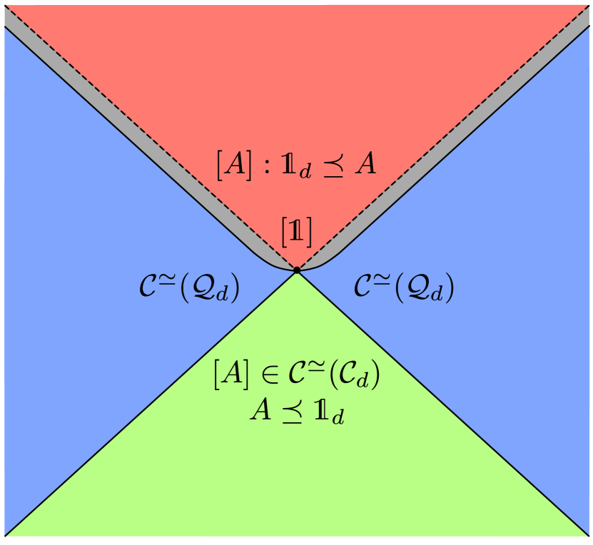
The sets of classical and quantum communication matrices can now be seen to share some structure; the identity matrix is a maximal element in both of them. We have seen that the identity is the greatest element in classical theory. With the following lemma we will prove our main result, namely that the identity is the only maximal element in quantum theory, although not the greatest. Our main result is illustrated in Fig. 3, which depicts the partially ordered set of communication matrices in light of Thm. 1.
Lemma 3.
Let , where , , are non-orthogonal 1-dimensional projections, , , and for some complex separable Hilbert space . The operator has two eigenvalues
where . An unnormalized eigenvector corresponding to the largest eigenvalue is .
Proof.
Let us calculate the eigenvalues of explicitly. Let . Then
| (6) |
This shows that the eigenvectors of are of the form for some complex numbers . Inserting into , we obtain
| (7) | ||||
| (8) |
where . Eliminating the variable yields
If , then the term inside the square root in the above equation must equal zero. Solving for in and requiring to be real ultimately yields which only holds for or as generally .
Finally, setting in Eq. (7), we get , so an unnormalized eigenvector corresponding to the eigenvalue is . We observe that if and only if and , . Notably an eigenvector of corresponding to is different from or whenever .
∎
Theorem 1.
Let . If is an ultraweakly maximal element in , then , i.e., is the only maximal element in .
Proof.
Suppose is maximal. Then and has an implementation , where ’s are either rank-1 or rank zero and the state ensemble contains the eigenstates of the non-zero effects of by Lemma 1. Observe that if the effects of are pairwise orthogonal, then is post-processing equivalent with a sharp rank-1 POM, and in this case by Prop. 2. Without loss of generality let us assume is incompressible.
Assume then that there exists a pair of effects, and , such that . Consider the following post-processing of these effects: , . We do not need to create the new effect via post-processing as we are able to calculate directly from the communication matrix for any . By Lemma 3 the positive operator has a singular maximal eigenvalue whenever . The eigenstate corresponding to this eigenvalue is a superposition of the eigenstates of and . Let us denote this state by . In particular, as is distinct from the eigenstates of and and approaches them as or , we conclude that there is an infinite number of possible eigenstates of corresponding to different values of and .
Let us now fix the values of and , . As was assumed maximal, we must have , where is formed from by adding to the state ensemble . We can always choose such and that is not already contained in the state ensemble. Note that it is not necessary for to contain as an effect. However, we have that is a unique solution. In particular this means that the row corresponding to in cannot be a convex combination of rows in .
The proof is now concluded by observing that and was incompressible. Therefore, if , then has an implementation with the state ensemble and a POM with the effects for some row-stochastic matrices and based on ultraweak majorization. Moreover, by Prop. 1, must be a permutation matrix. Hence the POM still contains the effects and although the outcomes might have been relabelled. Suppose these effects correspond to and so that . However, as we already concluded, is a unique solution where is the pure eigenstate of . Therefore it is not possible that as was not contained in the ensemble . This is a contradiction with the assumption that is maximal. Hence, it follows that the POM implementing is rank-1 and does not contain non-orthogonal effects, which by Prop. 2 implies .
∎
6. Discussion
Our main result showed that is the only maximal element in . The technique we used in our proof gives a mathematically intuitive reason for why this holds. Unless the quantum implementation of a communication matrix is done with a rank-1 sharp POM, we are always able to “strenghten” a communication matrix by adding new pure states into the state ensemble implementing it as long as there are at least some rank-1 effects. As there are infinitely many pure states in quantum theory of any dimension, we will never run out of possible new states to add. We thus run into these sequences of communication matrices , where each communication matrix is obtained from the previous by adding a state and each communication matrix in the sequence is genuinely stronger than the previous.
Although we are able to create these growing sequences of communication matrices, no quantum communication matrix is stronger than the identity. This result is surprising, yet in good agreement with Holevo’s theorem [34] which states that the information transmitted by a quantum system cannot exceed its operational dimension. It is important to stress that the set is not identical to . Therefore, contains communication matrices that are ultraweakly incomparable with . This was already pointed out in [22]. As is maximal it now follows that there must exist sets of incompatible communication matrices in .
Finally, we note that the question of maximal communication matrices can be studied in the framework of general probabilistic theories [35]. An open question is if classical and quantum theories are the only operational theories where the only maximal element is the identity. We leave this question, together with the question of incompatibility, for future works.
Acknowledgments
TH and OK acknowledge financial support from the Business Finland under the project TORQS, Grant 8582/31/2022, and from the Academy of Finland under the project DEQSE, Grant 349945.
References
- [1] C. H. Bennett and S. J. Wiesner. “Communication via one- and two-particle operators on Einstein-Podolsky-Rosen states”. Phys. Rev. Lett. 69, 2881 (1992).
- [2] C. H. Bennett, G. Brassard, C. Crépeau, R. Jozsa, A. Peres, and W. K. Wootters. “Teleporting an unknown quantum state via dual classical and Einstein-Podolsky-Rosen channels”. Phys. Rev. Lett. 70, 1895 (1993).
- [3] C. H. Bennett and G. Brassard. “Quantum cryptography: Public key distribution and coin tossing”. Theoretical Computer Science 560, 7 (2014).
- [4] S. Massar, D. Bacon, N. J. Cerf, and R. Cleve. “Classical simulation of quantum entanglement without local hidden variables”. Phys. Rev. A 63, 052305 (2001).
- [5] B. F. Toner and D. Bacon. “Communication cost of simulating bell correlations”. Phys. Rev. Lett. 91, 187904 (2003).
- [6] M. J. Renner, A. Tavakoli, and M. T. Quintino. “Classical cost of transmitting a qubit”. Phys. Rev. Lett. 130, 120801 (2023).
- [7] A. Ambainis, D. Leung, L. Mancinska, and M. Ozols. “Quantum random access codes with shared randomness” (2009). arXiv:0810.2937.
- [8] T. Guha, M. Alimuddin, S. Rout, A. Mukherjee, S. S. Bhattacharya, and M. Banik. “Quantum Advantage for Shared Randomness Generation”. Quantum 5, 569 (2021).
- [9] R. Gallego, N. Brunner, C. Hadley, and A. Acín. “Device-independent tests of classical and quantum dimensions”. Phys. Rev. Lett. 105, 230501 (2010).
- [10] R. Chaves, J. B. Brask, and N. Brunner. “Device-independent tests of entropy”. Phys. Rev. Lett. 115, 110501 (2015).
- [11] S. Saha, S. S. Bhattacharya, T. Guha, S. Halder, and M. Banik. “Advantage of quantum theory over nonclassical models of communication”. Annalen der Physik 532, 2000334 (2020).
- [12] H. Buhrman, R. Cleve, J. Watrous, and R. de Wolf. “Quantum fingerprinting”. Phys. Rev. Lett. 87, 167902 (2001).
- [13] A. Ambainis, A. Nayak, A. Ta-Shma, and U. Vazirani. “Dense quantum coding and quantum finite automata”. J. ACM 49, 496 (2002).
- [14] C. Perry, R. Jain, and J. Oppenheim. “Communication tasks with infinite quantum-classical separation”. Phys. Rev. Lett. 115, 030504 (2015).
- [15] P. Emeriau, M. Howard, and S. Mansfield. “Quantum advantage in information retrieval”. PRX Quantum 3, 020307 (2022).
- [16] E. F. Galvão and L. Hardy. “Substituting a qubit for an arbitrarily large number of classical bits”. Phys. Rev. Lett. 90, 087902 (2003).
- [17] T. Heinosaari, O. Kerppo, L. Leppäjärvi, and M. Plávala. “Simple information processing tasks with unbounded quantum advantage” (2023). arXiv:2308.07727.
- [18] P. W. Shor. “Polynomial-time algorithms for prime factorization and discrete logarithms on a quantum computer”. SIAM Journal on Computing 26, 1484 (1997).
- [19] F. Arute et al. “Quantum supremacy using a programmable superconducting processor”. Nature 574, 505 (2019).
- [20] F. Pan and Pan P. Zhang. “Simulation of quantum circuits using the big-batch tensor network method”. Phys. Rev. Lett. 128, 030501 (2022).
- [21] T. Heinosaari and O. Kerppo. “Communication of partial ignorance with qubits”. J. Phys. A: Math. Theor. 52, 395301 (2019).
- [22] T. Heinosaari, O. Kerppo, and L. Leppäjärvi. “Communication tasks in operational theories”. J. Phys. A: Math. Theor. 53, 435302 (2020).
- [23] G. Kimura, K. Nuida, and H. Imai. “Distinguishability measures and entropies for general probabilistic theories”. Rep. Math. Phys. 66, 175 (2010).
- [24] S. Bandyopadhyay, R. Jain, J. Oppenheim, and C. Perry. “Conclusive exclusion of quantum states”. Phys. Rev. A 89, 022336 (2014).
- [25] C. M. Caves, C. A. Fuchs, and R. Schack. “Conditions for compatibility of quantum-state assignments”. Phys. Rev. A 66, 062111 (2002).
- [26] T. Heinosaari and O. Kerppo. “Antidistinguishability of pure quantum states”. J. Phys. A: Math. Theor. 51, 365303 (2018).
- [27] J. E. Cohen and U. G. Rothblum. “Nonnegative ranks, decompositions, and factorizations of nonnegative matrices”. Linear Algebra Appl. 190, 149 (1993).
- [28] H. Fawzi, J. Gouveia, P. A. Parrilo, R. Z. Robinson, and R. R. Thomas. “Positive semidefinite rank”. Mathematical Programming 153, 133 (2015).
- [29] T. Lee, Z. Wei, and R. de Wolf. “Some upper and lower bounds on psd-rank”. Math. Program. 162, 495 (2017).
- [30] K. Matsumoto and G. Kimura. “Information storing yields a point-asymmetry of state space in general probabilistic theories” (2022). arXiv:1802.01162.
- [31] B. Schumacher and M. Westmoreland. “Quantum processes, systems, and information”. Cambridge University Press, Cambridge. (2010).
- [32] O. Kerppo. “Quantum communication tasks”. PhD thesis. University of Turku. (2023). url: https://urn.fi/URN:ISBN:978-951-29-9127-3.
- [33] F. D. Martínez Pería, P. G. Massey, and L. E. Silvestre. “Weak matrix majorization”. Linear Algebra Appl. 403, 343 (2005).
- [34] A. S. Holevo. “Bounds for the quantity of information transmitted by a quantum communication channel”. Probl. Peredachi Inf. 9, 3 (1973). url: https://www.mathnet.ru/eng/ppi903.
- [35] M. Plávala. “General probabilistic theories: An introduction”. Physics Reports 1033, 1 (2023).
