STATISTICAL INFERENCE FOR A SERVICE SYSTEM WITH NON-STATIONARY ARRIVALS AND UNOBSERVED BALKING

Abstract

We study a multi-server queueing system with a periodic arrival rate and customers whose joining decision is based on their patience and a delay proxy. Specifically, each customer has a patience level sampled from a common distribution. Upon arrival, they receive an estimate of their delay before joining service and then join the system only if this delay is not more than their patience, otherwise they balk. The main objective is to estimate the parameters pertaining to the arrival rate and patience distribution. Here the complication factor is that this inference should be performed based on the observed process only, i.e., balking customers remain unobserved. We set up a likelihood function of the state dependent effective arrival process (i.e., corresponding to the customers who join), establish strong consistency of the MLE, and derive the asymptotic distribution of the estimation error. Due to the intrinsic non-stationarity of the Poisson arrival process, the proof techniques used in previous work become inapplicable. The novelty of the proving mechanism in this paper lies in the procedure of constructing i.i.d. objects from dependent samples by decomposing the sample path into i.i.d. regeneration cycles. The feasibility of the MLE-approach is discussed via a sequence of numerical experiments, for multiple choices of functions which provide delay estimates. In particular, it is observed that the arrival rate is best estimated at high service capacities, and the patience distribution is best estimated at lower service capacities.

Keywords. Service systems $\circ$ balking $\circ$ periodic arrivals $\circ$ estimation $\circ$ customer patience

Affiliations. SAB is with the Korteweg-de Vries Institute for Mathematics, University of Amsterdam, Science Park 904, 1098 XH Amsterdam, The Netherlands. s.a.bodas@uva.nl

MM is with the Mathematical Institute, Leiden University, P.O. Box 9512, 2300 RA Leiden, The Netherlands. He is also affiliated with Korteweg-de Vries Institute for Mathematics, University of Amsterdam, Amsterdam, The Netherlands; Eurandom, Eindhoven University of Technology, Eindhoven, The Netherlands; Amsterdam Business School, Faculty of Economics and Business, University of Amsterdam, Amsterdam, The Netherlands. m.r.h.mandjes@math.leidenuniv.nl

LR is with the Department of Statistics, University of Haifa, 199 Aba Khoushy Avenue, Mount Carmel, Haifa, Israel. lravner@stat.haifa.ac.il

Acknowledgments. This research was supported by the European Union’s Horizon 2020 research and innovation programme under the Marie Skłodowska-Curie grant agreement no. 945045, by the NWO Gravitation project NETWORKS under grant agreement no. 024.002.003 and by the Israel Science Foundation (ISF), grant no. 1361/23. Date: .

INTRODUCTION

In our modern world, customers interact with service systems on a daily basis. Examples abound across a broad range of economic sectors: besides conventional shops, one can think of online delivery services, communication and computing networks, call centers, and various types of healthcare systems. Seen from a conceptual perspective, in these systems the service capacity is a scarce resource, for which customers compete. When these customers are provided information on the current occupancy level, they may find the anticipated service level too poor, so that they decide not to join, a phenomenon known as ‘balking’. Such balking decisions are typically made based on an estimate of the delay the customer under consideration would be facing, or, more generally, the performance level they would receive.

When operating a service system, it is of crucial importance to have an accurate quantitative description of its underlying dynamics. Often one resorts to a queueing-theoretic framework, encompassing a customer arrival process, a specification of the service requirements, and a service mechanism. In a practical context, this means that the ‘model primitives’ are estimated, by performing statistical inference based on observations of the system over time. A frequently overlooked complication, however, is that often balking customers remain unobserved. Despite the fact that balking customers do not join the system, a system operator still wishes to reliably estimate the effective arrival rate, i.e., the rate of joining customers plus the rate of balking customers. The reason why this total arrival rate is relevant, is that it reflects the demand for the service, which is of key importance in decisions concerning e.g. staffing, dimensioning or pricing. Healthcare service providers, for instance, could use knowledge of the total demand to decide whether extra doctors or beds are required. Along the same lines, delivery services could consider a price adjustment so as to enlarge their market share.

A second complication that is ignored in many studies, is that the demand for service often fluctuates with time, typically following daily or weekly patterns; see for instance [14, 17] for analyses in the call center context. This means that while many modelling frameworks assume a time-independent Poissonian effective arrival rate, it would be more natural to work with a rate that follows some periodic pattern.

When setting up an estimation approach, one would like to be sure it provides reliable output. This concretely means that, ideally, the proposed estimator is consistent (i.e., converge to the true values when the sample size grows large), while in addition we would like to have insight into its asymptotic properties (for instance by proving that the estimator is asymptotically normally distributed).

The main conclusion from the above considerations, is that there is a clear need for a robust methodology to statistically estimate the service system’s model parameters. To make sure it can be used in an operational context, it should fulfil the following three requirements: (a) it should be based on observable data only, i.e., data corresponding to the joining customers, (b) it should be able to deal with a non-constant effective arrival rate, and (c) the proposed procedure should be equipped with provable performance guarantees.

In this paper we choose to model the service system as a first-come-first-served queue of the M_t/G/$s$+H type. We have selected this class of models because of its generality, capturing a broad range of relevant service systems. It can be described as follows:

• In the first place, customers arrive according to a non-homogeneous periodic Poissonian arrival rate $\lambda_{{\bm{\alpha}}}(\cdot)\geq 0$. Acknowledging that this rate typically follows a daily (or weekly) pattern, we throughout impose the natural assumption that we know the length of the corresponding period. In our setup we develop a parametric inference procedure: we let the arrival rate be parametrized by an unknown (finite-dimensional) parameter vector ${\bm{\alpha}}$.

• Each customer brings along a random amount of work. These service requirements for an i.i.d. sequence of non-negative random variable, with cumulative distribution function $G(\cdot)$, sampled independently of the arrival process.

• There are $s\in{\mathbb{N}}$ servers who serve in a first-come-first-serve manner. As it is a design parameter that is under full control of the service provider, throughout this paper we assume we know $s$.

• Our system explicitly takes into account the option of balking by incorporating the following impatience mechanism. Each arriving customer is equipped with a patience level, sampled independently of everything else. The customers’ patience levels are i.i.d., distributed as the non-negative random variable $Y$, characterized through the cumulative distribution function $H_{{\bm{\theta}}}(\cdot)$. Again, we work in a parametric context, with ${\bm{\theta}}$ representing the underlying (finite-dimensional) parameter vector. Upon arrival, and before joining, customers observe the state of the system, which they use to estimate the delay that they will be experiencing. By comparing this delay estimate with their patience, they decide to join or to balk.

• In this paper we consider multiple flavors of the balking mechanism. In certain systems, it is possible for customers to observe the workload, so that they know their exact prospective delay; think of a communication network in which any customer is provided with the volume of traffic to be processed prior to the commencement of their service. In other systems, however, customers are only given information on the number of customers in the system, which they can use to estimate the delay; think of a call center or a physical shop. Once a customer joins the system, they do not leave until service completion.

In the context of this M_t/G/$s$+H setup, our concrete objective is to devise a procedure, endowed with provable performance guarantees, to estimate the parameter vector $({\bm{\alpha}},{\bm{\theta}})$ governing the arrival rate and the patience distribution, relying on information regarding the non-balking customers only. Our procedure is based on maximum likelihood estimation (MLE), exploiting that the system’s key dynamics are dictated by the state-dependent effective arrival rate in the following way. Suppose that at a given point in time, which we associate for ease with time $0$, the virtual waiting time is $v$; this virtual waiting time is defined as the waiting time of a hypothetical customer joining at time $0$. If there are no effective arrivals in $(0,t]$, then the virtual waiting time at time $t$ is $(v-t)^{+}$, so that the effective arrival rate at time $t$ becomes

$$\lambda_{{\bm{\alpha}}}(t)\big{(}1-H_{{\bm{\theta}}}((v-t)^{+})\big{)}.$$

Observe how this arrival rate depends both on time as well as the state of the system (or, more concretely, the current congestion level). Various other variants can be thought of, such as the above-mentioned mechanism in which the number of customers (seen upon arrival) is observed, rather than the exact virtual waiting time. Note that in the latter case, between successive events (which can be arrivals or departures), the arrival rate depends only on time. The idea is then that once we know the state-dependent effective arrival rate, we can calculate the distribution of the effective interarrival times conditioned on the system state, which we use to produce a closed-form expression for the conditional log-likelihood of the arrival process.

When attempting to estimate $({\bm{\alpha}},{\bm{\theta}})$, there are various additional complications to be dealt with. An important challenge is that when the non-homogeneous arrival rate is significantly greater than the service capacity, the system operator only observes the joining customers may incorrectly conclude that the arrival rate is a small constant, as explained in Example 1.1. Another challenge concerns the (possible lack of) identifiability of the arrival and patience distribution functions with respect to the parameters, as explained in Example 1.2.

Example 1.1.

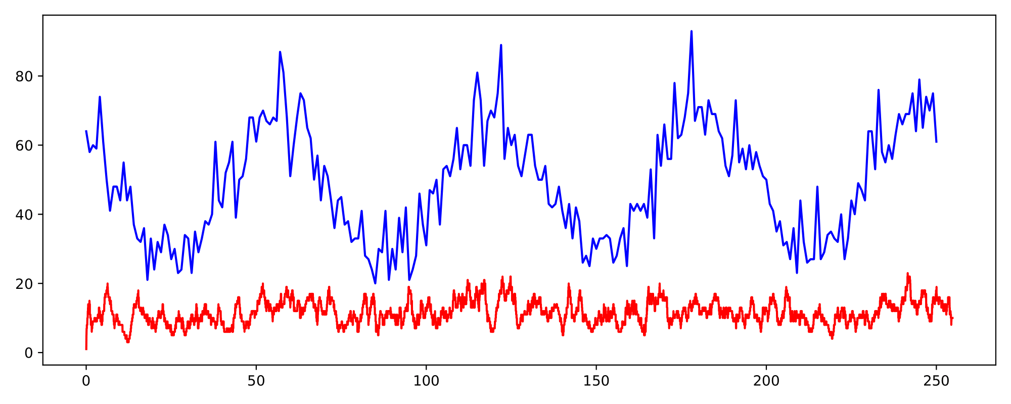
(a) $s=1$, balk = 90%

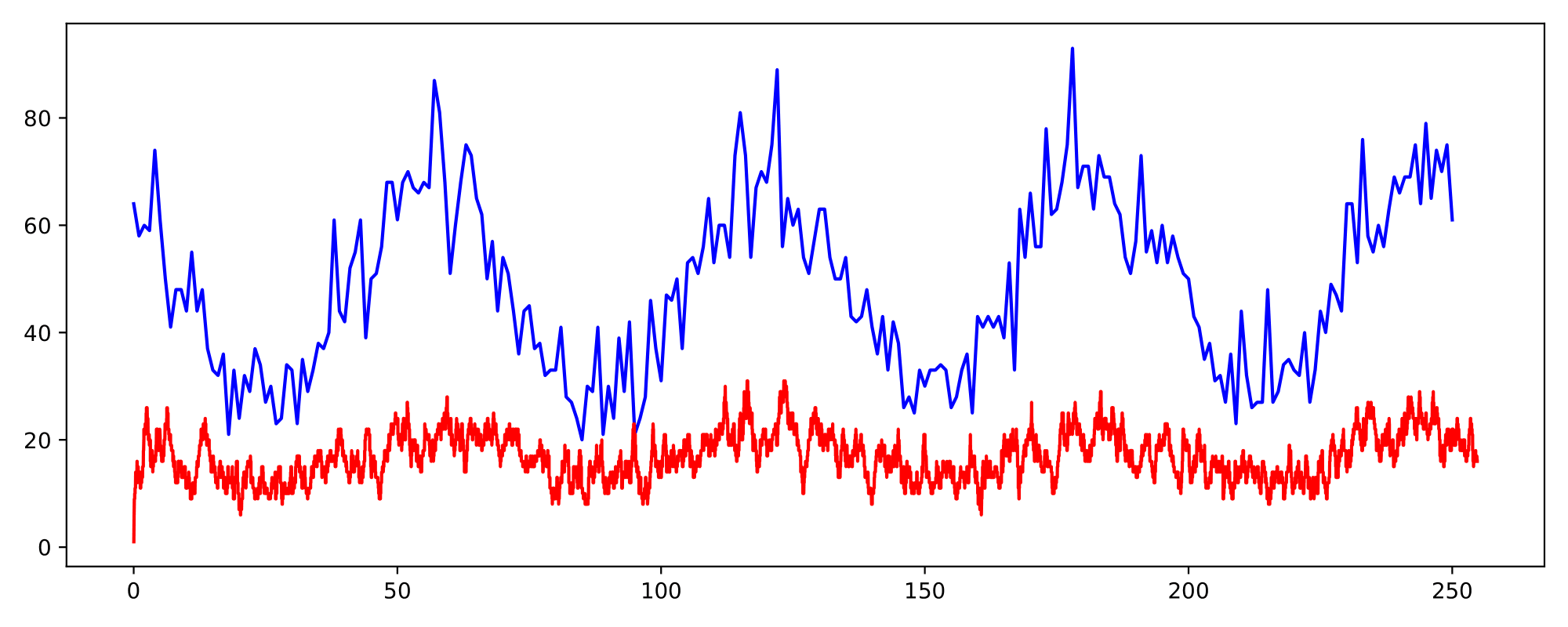
(b) $s=2$, balk = 80%

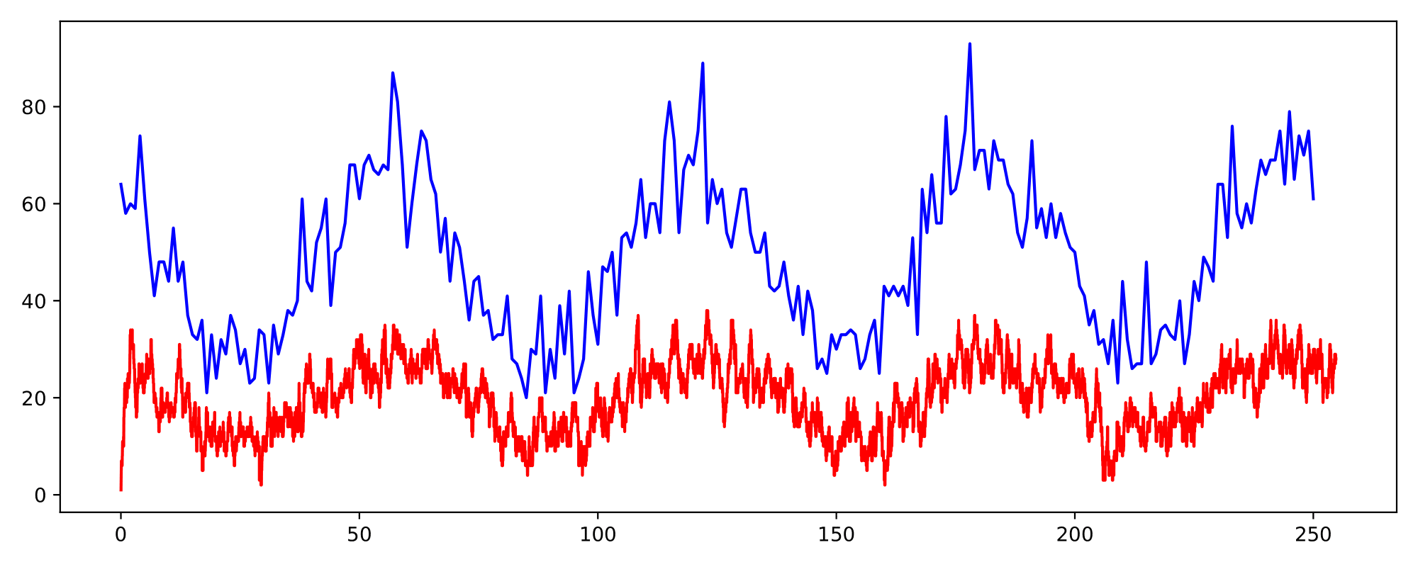
(c) $s=4$, balk = 60%

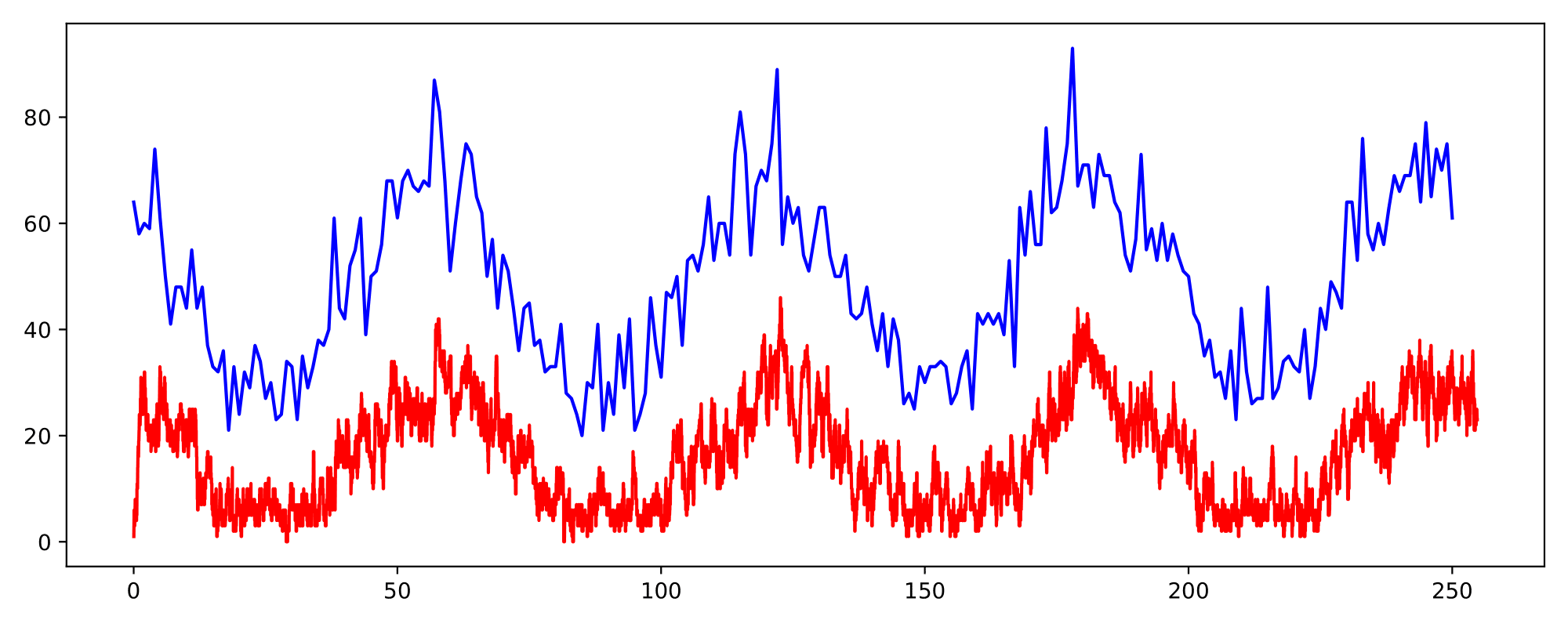
(d) $s=8$, balk = 25.7%

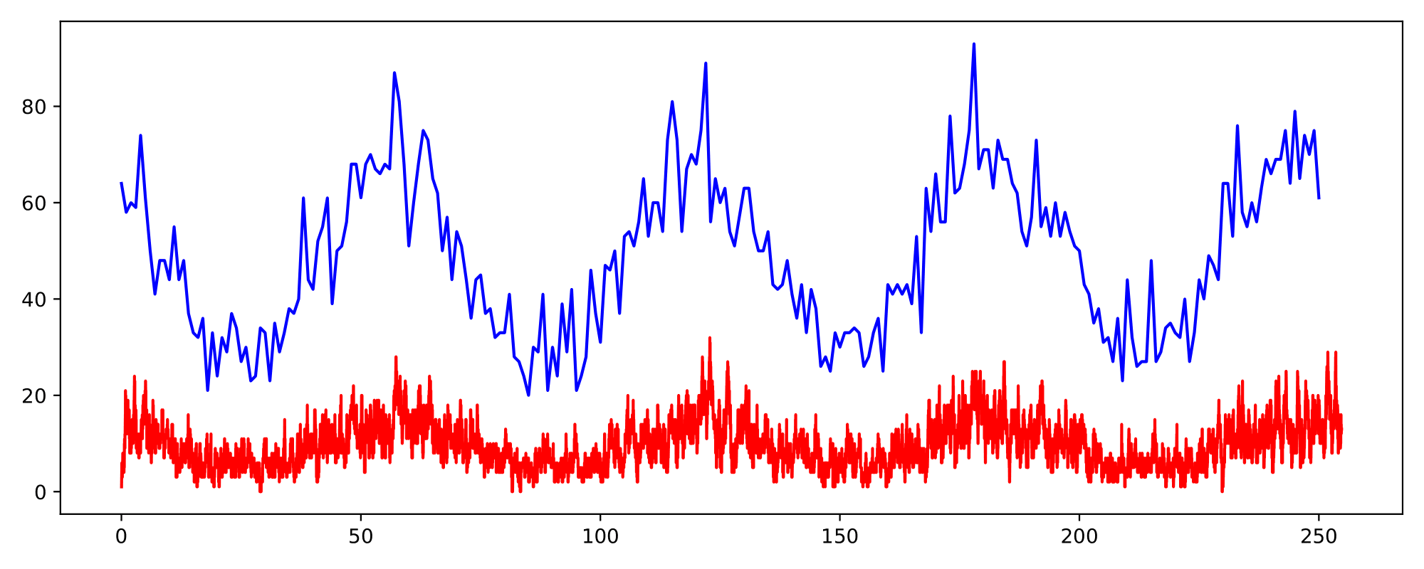
(e) $s=16$, balk = 0.8%

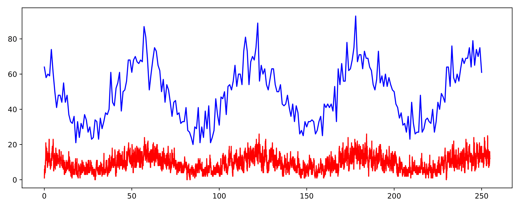
(f) $s=32$, balk = 0%

Figure 1: Effect of impatience and service capacity on state of system. Here ‘balk’ is the percentage of customers balking. Blue lines represents the arrival rate, and red lines the number of customers in the system

Figure 1 shows the time evolution of six M_t/G/$s$+H systems. We throughout assume that the arrival rate is given through a sinusoidal with period $20\,\pi$, given by $\lambda_{{\bm{\alpha}}_{0}}(t)=50+20\sin(1-0.1t)$. Both the patience distribution function $H_{{\bm{\theta}}_{0}}(\cdot)$ and the service requirements distribution function $G(\cdot)$ are taken exponentially with mean 1. The number of servers we vary: we consider $s\in\{1,2,4,8,16,32\}$. The specific realizations of the arrival times, service requirements, and patience times are kept unchanged across all experiments.

The blue line is a realization of the empirical arrival process with rate $\lambda_{{\bm{\alpha}}_{0}}(t)$. For each integer-valued time point $n$, the y-coordinate of the blue line represents the total number of arrivals (balking plus non-balking, that is) that have occurred in $[n,n+1)$. The red line plots the number of customers in the system as a function of time.

We proceed by examining how the red line behaves across the six instances. For the cases $s=1$ and $s=2$, the waiting times are so high that a dominant fraction of customers balk. By observing only the red line in Figures 1(a) and 1(b), one cannot infer that that the arrival rate is actually large and non-homogeneous. In fact, if the administrator is unaware of balking they may even conclude that the arrival process is stationary and not time-dependent. Furthermore, from a statistical perspective, balking customers help estimate the patience parameters ${\bm{\theta}}_{0}$, but not the arrival rate parameters ${\bm{\alpha}}_{0}$. On the other hand, for the cases $s=16$ and $s=32$, the service capacity is much higher than the arrival rate and therefore, so that only a negligible percentage of the arriving customers balk. As a consequence, the estimates of ${\bm{\alpha}}_{0}$ are precise whereas those of ${\bm{\theta}}_{0}$ are poor. In a way, the ‘best’ instances are therefore the middle ones (i.e., $s=4$ and $s=8$), where both ${\bm{\alpha}}_{0}$ and ${\bm{\theta}}_{0}$ allow a reasonably accurate estimation. $\Diamond$

Figure 2: Identifiability challenge while estimating patience distribution

Example 1.2.

We simulate an M_t/G/$s$+H queue characterized by $\lambda_{{\bm{\alpha}}_{0}}(t)=50+15\sin(4-0.1t)+10\sin(1-0.5t)$, $H_{{\bm{\theta}}_{0}}(x)=1-0.8e^{-x}-0.2e^{-0.1x}$, $G\sim\text{Exp}(0.4)$, and $100\,000$ arrivals (balking plus non-balking, that is). The true parameter vectors are therefore ${\bm{\alpha}}_{0}=(50,15,10,4,1)$ and ${\bm{\theta}}_{0}=(0.8,1,0.1)$. By applying our estimation procedure, described later in this paper, the estimates that we obtain are $\hat{{\bm{\alpha}}}=(49.44,14.95,10.41,4.00,0.98)$ and $\hat{{\bm{\theta}}}=(0.85,0.91,0.05)$. Observe that $\hat{{\bm{\alpha}}}$ is reasonably accurate, whereas $\hat{{\bm{\theta}}}$ is relatively far from ${\bm{\theta}}_{0}$. However, now observe in Figure 2, where the blue and red lines plot the distribution functions $H_{{{\bm{\theta}}_{0}}}(x)$ and $H_{\hat{{\bm{\theta}}}}(x)$ respectively, that the estimate $\hat{{\bm{\theta}}}$ being inaccurate does not mean that the corresponding estimate $H_{\hat{{\bm{\theta}}}}(x)$ is. Put differently, the inaccuracy in the estimation of ${\bm{\theta}}_{0}$ is in a way harmless, because $H_{{\bm{\theta}}_{0}}(x)$ is estimated with great precision. One could say that we are facing a ‘quasi-unidentifiability’ issue: multiple parameter vectors lead to ‘almost identical’ models.

The system’s congestion level plays a crucial role in the ability to accurately estimate the patience parameters. In this simulation the maximum virtual waiting time observed by a customer is 5.304. This is less than 6, which is, as revealed by Figure 2, the value beyond which one can really differentiate between $H_{{\bm{\theta}}_{0}}(x)$ and $H_{\hat{{\bm{\theta}}}}(x)$. When increasing the number of arrivals, the maximum observed virtual waiting time will increase, thus reducing the gap between $\hat{{\bm{\theta}}}$ and ${\bm{\theta}}_{0}$. $\Diamond$

Contributions

This paper succeeds in devising an estimation methodology that fulfils the requirements (a), (b), and (c) defined above. The proposed approach parametrically estimates the arrival rate and patience distribution parameter vectors $({\bm{\alpha}},{\bm{\theta}})$ in an M_t/G/$s$+H system by only observing information associated with the non-balking customers. It thus extends previous work [18] by incorporating a time-dependent customer arrival rate. Due to this time-dependence one cannot use a proof technique in which one has assumed that the system has reached stationarity. In greater detail, the contributions are the following:

• Our estimation procedure is based on maximum likelihood. One would initially think that such an approach should make use of closed-form (transient or stationary) results for the M_t/G/$s$+H queue, but those are hardly available; even the (simpler) M/G/$s$ system is essentially intractable. We circumvent this problem, however, by constructing a closed-form expression for the conditional log-likelihood pertaining to the state-dependent arrival process.

• As mentioned before, due to the periodic arrival rate, one cannot assume the system to be in stationarity. We remedy this complication by decomposing the sample path of the queueing system variables into distinct regeneration cycles, which are periods of time after which the system probabilistically resets. This allows us to introduce, out of sequences of dependent observations, an i.i.d. structure, thus facilitating the use of existing results (laws of large numbers, central limit theorems) so as to establish performance guarantees of the resulting estimator. For arrival rate functions and patience distributions satisfying mild regularity conditions and under other natural assumptions, we prove the strong consistency of the maximum likelihood estimator. We also prove asymptotic normality of the corresponding estimation error (scaled by $\sqrt{n}$), which is the fastest convergence rate possible in a parametric setting.

  In addition, we have developed a number of verifiable assumptions, based solely on the model primitives, under which the above asymptotic analysis is valid.

• Our model allows arriving customers to base their joining decision on any reasonable function of the complete state of the system. That is, upon arrival, they do not necessarily need to know their precise waiting time. In particular, suppose a customer with patience level $Y$ arrives at time $t$ and let $\mathcal{R}(t)\in\Omega$ encode the full information of the system at time $t$ (for example, the residual service times and order of service for all customers present in the system at time $t$), and let $\psi:\Omega\mapsto\mathbb{R}$ be a Borel function. Then one can use the rule that a customer joins the system only if $Y\geq\psi(\mathcal{R}(t))$. Concrete examples of such a function $\psi(\cdot)$ include the exact or noisy estimates of the expected waiting time or the number of customers in the system. An important example is that in which any customer (say, arriving at time $t$) bases their decision on the number of customers (say $q$) in the system seen upon arrival. If $q<s$, then there is at least one idle server and hence the delay before getting into service is $0$. If $q\geq s$, then a (biased, but probably reasonable) estimate of this delay could be $(q-s+1)g/s$, where $g$ is the mean service time. We can compile this into an information function of the form $\psi(\mathcal{R}(t))=(L(t)-s+1)^{+}g/s$, where $L(t)$ is the number of customers in the system at time $t$.

• We discuss several interesting insights obtained from numerical experiments, such as the identification of instances where estimation of $({\bm{\alpha}}_{0},{\bm{\theta}}_{0})$ is intrinsically hard (cf. the discussion in Example 1.1), and how ‘near-unidentifiability’ issues play a role in estimation (cf. the discussion in Example 1.2). We also assess the estimation accuracy in situations when exact virtual waiting times are not known.

Relevant Literature

This paper remedies two key shortcomings of the predecessor paper [18], where estimation of constant arrival rate and patience distribution was carried out in the context of service system modelled by an M/G/$s$+H queue. In the first place, we lift the assumption of the customer arrival rate being constant over time by allowing a periodic arrival rate. Second, [18] assumes a complete information setting, in that each arriving customer knows their exact prospective waiting time, which is often infeasible in practical situations. Importantly, our paper demonstrates that our estimation technique works even when customers have incomplete information, and estimate their prospective waiting time based on a partially observed system state.

An intensively studied topic at the intersection of operations research, applied probability and statistics, concerns the estimation of model primitives based on the (potentially partially observed) evolution of a stochastic process. For instance, [35] estimates distribution functions with truncated data. A specific subfield focuses on inference problems for queues, where the objective is to estimate the input process based on queue length or workload observations; see for instance the detailed survey [2]. Each study in this survey is characterized by its own specific underlying model, observation process, and estimation objectives. For instance, [5] studies an M/G/$\infty$ system, observing specific aspects of the evolution of the number of customers present, with the objective to estimate the arrival rate and service-time distribution (making the problem semi-parametric). In [33] the M/M/$s$ queue length is observed in the regime that $c$ is large $c$, and employs a diffusion approximation for estimating the arrival and service rates. In [23] one observes the so-called transactional data (i.e., times of service initiations and completions), and based on these one estimates various queue-related statistics. In [32] the workload process of a Lévy-driven queue is sampled at Poisson instants, providing observations that can be used in a method-of-moments estimator for the characteristic exponent of the driving Lévy process. Finally, [31] studies a discrete time M/G/$\infty$ queue with the objective of estimating the arrival rate and service distribution. It uses an entropy-motivated geometric approximation to employ algorithms used for estimation of hidden Markov models. In general one aims to develop estimation techniques with certain concrete performance guarantees, in particular consistency or asymptotic normality.

A complication we come across in our setting with impatient customers, is that we wish to estimate the total arrival rate, i.e., including the arrival rate corresponding to the customers that balk due to impatience. In the queueing literature, impatience has been studied from several perspectives; in line with the focus of the present paper, we discuss work in which balking is due to arriving customers facing a high prospective waiting time. In [3] stability condition is established for M_t/G/1+H systems with a periodic arrival rate. Then, [24] derives the steady-state workload distribution, and hence implicitly also a stability condition, for the M/Ph/1 queue (in which service requirements are of phase type) with a constant patience level across all customers. In [25] the Laplace-Stieltjes transform of the busy period of M/Ph/1 queues is derived, as a limiting case of an associated fluid model. In [7] the busy period distribution in an M/G/1+H system is identified, for various choices of patience distribution $H(\cdot)$. The problem of estimating customer (im)patience in service systems has also been given significant attention; see e.g., [26], while further references can be found in [18].

Time-varying multi-server queues also have attracted some attention in the queueing literature. Where [34] provides an extensive bibliography on queues time-varying arrival rates, we highlight some key works. In [28] the focus is on the distribution of the number of busy servers in an M_t/G/$s$/$0$ loss system, which has $s$ servers and no extra waiting space (i.e. there can be at most $s$ customers in the system at any time) and a non-homogeneous Poisson arrival process, using a modified offered-load approximation. Reference [29] studies the asymptotic behaviour of arrival, departure and waiting times in unstable queues with non-stationary arrival rates. A branch of research focuses on estimation; in this context, [27] studies the approximation of a non-homogeneous arrival rate by a piecewise linear counterpart. In [20] a time-varying Little’s law is used to develop estimators for waiting times in systems with time-varying arrival rates. The main objective of [19] lies in staffing: it presents an algorithm to select the number of servers as a function of time, so as to meet given performance targets. In [8] it is shown that periodic sinusoidal arrival rates have a good empirical fit with arrival data from various service systems.

Poisson processes play a pivotal role in queueing theory, primarily with a constant rate, but the case of a time-dependent rate has received substantial attention as well. In the statistics literature, the case of non-homogeneous, potentially periodic, Poisson processes has been covered by for instance [10, 11, 12, 21, 36]; these papers differ in terms of the underlying model (which can be either parametric or non-parametric), the nature of the observation process, and the estimation technique relied upon. A textbook treatment of inference techniques for broad classes of Poisson processes can be found in [22].

We conclude this account of the existing literature by mentioning a number of works that have been used in our consistency and asymptotic normality proofs. In the first place, we rely on results that provide insight into our M_t/G/$s$+H queue; in particular, [13] shows how the regeneration cycles can be dealt with in time-varying queues. In addition, we use results from [1] in our strong consistency proof, and results from [4] on establishing the recurrence of specific sets (by which we can derive properties which play a key role in our proofs).

Paper Organization

In Section 2, we provide a model description and present preliminaries. Section 3 details the MLE-based estimator, along with theorems regarding their strong consistency and asymptotic normality. From the methodological perspective, Section 4 can be seen as the heart of this paper: we describe our procedure to decompose the sample path into distinct regeneration cycles, which is a central element in the proofs in Section 5. Section 5 also contains an exhaustive list of model assumptions under which the theorems and proofs hold. In Section 6, we discuss a general model framework where each customer at the time of joining does not know their exact waiting time but rather uses a proxy. We establish here that strong consistency and asymptotic normality of the estimators is valid even in this general setting. In Section 8, we discuss our findings, and provide directions for future research. Section 7 contains a series of simulation experiments, confirming our estimation procedure’s efficacy. In Appendix A, we prove results related to a regeneration structure underlying the M_t/G/$s$+H system, which are required in our proofs. Appendix B contains proofs some lemmas that are required in the proofs of consistency and asymptotic normality.

MODEL AND PRELIMINARIES

For the sake of simplicity and ease of reading, for now, we consider the framework in which arriving customers are given exact information regarding their waiting time. We do note, however, that the estimation procedure and subsequent asymptotic analysis can be carried out even when this is not assumed. In this and the next sections we work under the ‘exact information assumption’, but in Section 6 we discuss how similar computations can be performed to obtain estimators in setups where the joining decision relies on noisy estimates of the waiting time, or on observations of the number of customers present in the system.

We model our service system via a queue with $s\in{\mathbb{N}}$ servers. Potential customers arrive according to a Poisson process with a time-dependent arrival rate $\lambda_{{\bm{\alpha}}}(t)$, parametrized by the vector ${\bm{\alpha}}\equiv(\alpha_{1},\alpha_{2},\ldots,\alpha_{k})\in\mathbb{R}^{k}$ for some $k\in{\mathbb{N}}$. We consider the setting in which the arrival rate is periodic, where the period is known; by normalizing time we can assume without loss of generality the period is one, so that $\lambda_{{\bm{\alpha}}}(t+1)=\lambda_{{\bm{\alpha}}}(t)$ for all $t\geq 0$. Each customer is equipped with (1) a service requirement that has cumulative distribution function $G(\cdot)$, and (2) a patience level that has cumulative distribution function $H_{{\bm{\theta}}}(\cdot)$, where ${\bm{\theta}}\equiv(\theta_{1},\theta_{2},\ldots,\theta_{p})\in\mathbb{R}^{p}$ (for some $p\in{\mathbb{N}}$) represent the parameters of the patience distribution. The service requirements $\{B_{i}\}_{i\in{\mathbb{N}}}$ and patience levels $\{Y_{i}\}_{i\in{\mathbb{N}}}$ are independent sequences of i.i.d. random variables, and the customer interarrival times $\{T_{i}\}_{i\in{\mathbb{N}}}$ are independent of $\{B_{i}\}_{i\in{\mathbb{N}}}$ and $\{Y_{i}\}_{i\in{\mathbb{N}}}$. Note that the interarrival times are neither independent of each other, nor identically distributed because of the arrival rate varying with time.

We proceed by detailing the balking mechanism. Customer $i$ joins the system if and only if their patience $Y_{i}$ is greater than or equal to their prospective waiting time. More specifically, let $V(t)$ denote the virtual waiting time at time $t\geq 0$, which is defined as the waiting time experienced by a hypothetical customer who joins the system immediately after time $t$. The quantity $V(t)$ can alternatively be understood as the time it would take before at least one server becomes idle if no customers join the system after time $t$. That is, for any $t\geq 0$, the virtual waiting time can be defined by

$$V(t)=\inf\big{\{}u\geq 0:L(t)-\big{(}N_{D}(t+u)-N_{D}(t)\big{)}\leq s-1\big{\}}$$ (2.1)

where $L(t)$ is the number of customers in the system (including those in service) at time $t$, and $N_{D}(t)$ the total number of customers that have finished their service by time $t$. The virtual waiting time process $\{V(t)\}_{t\in{\mathbb{R}}}$ is a càdlàg (‘right continuous with left limits’) process. Customer $i\in{\mathbb{N}}$ joins the system if their patience is at least equally large as their virtual delay:

$$Y_{i}\geq V\Biggl{(}\sum_{j=1}^{i}T_{j}-\Biggr{)}.$$ (2.2)

Figure 3 provides an illustration of the virtual waiting time process of an M/G/2+H queueing system with (for ease) a constant arrival rate $\lambda=10$, service requirements with unit mean, and patience levels that are deterministically equal to 1. The green (red) dots represent the non-balking (balking, respectively) customers. In the graph the virtual waiting time just prior to the arrival of non-balking (balking) customers is smaller (larger, respectively) than 1.

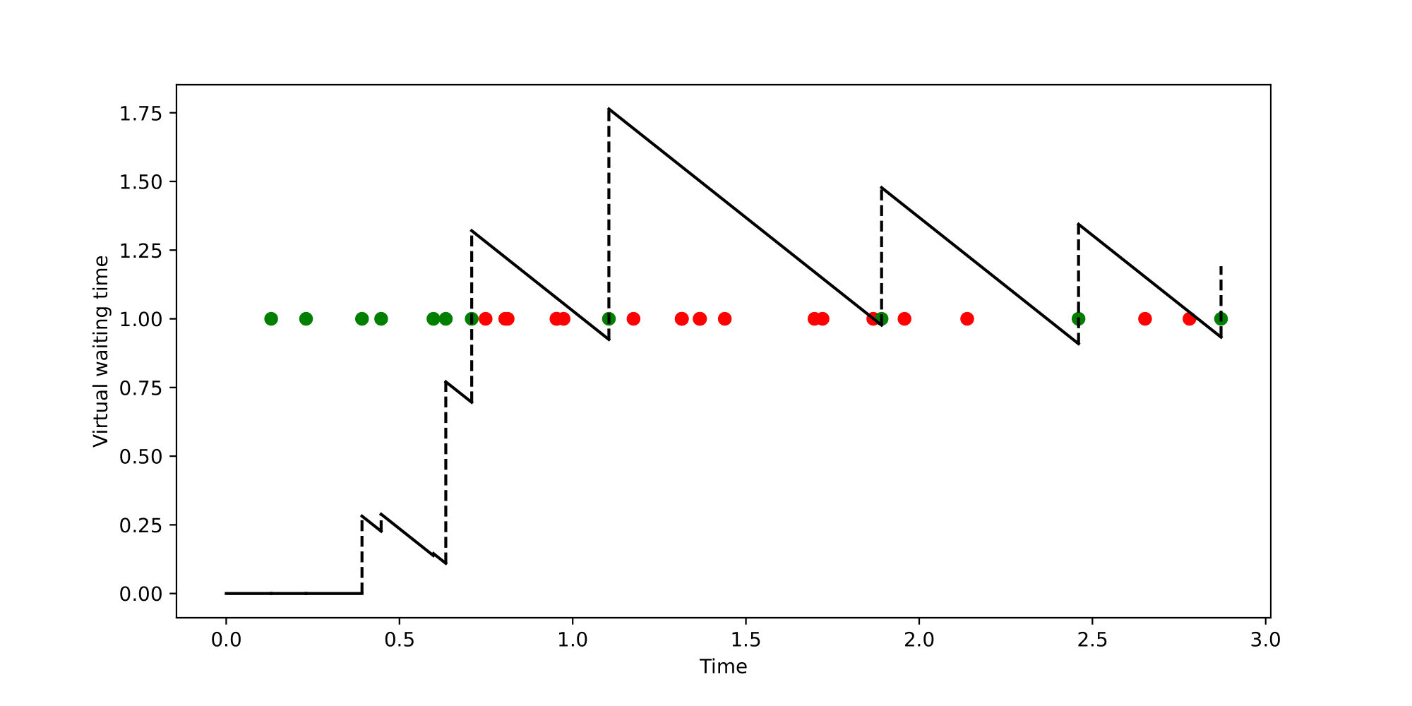
Figure 3: An example of virtual waiting time process $(s=2)$ and joining decisions of customers

We now discuss the inference problem addressed in this paper. The crucial feature is that only non-balking customers can be observed, i.e., the customers corresponding to the green dots in Figure 3. Our estimation procedure relies on the state dependent distribution of the effective interarrival times, i.e., the times between two subsequent non-balking arrivals. In the sequel, we denote the sequence of effective interarrival times by $\{A_{i}\}_{i\in{\mathbb{N}}}$, and the corresponding effective arrival times by $\{\tilde{A}_{i}\}_{i\in{\mathbb{N}}}$, i.e., $\tilde{A}_{i}=\sum_{j=1}^{i}A_{j}$. Each non-balking arrival causes a non-negative increase in the virtual waiting time, which we can be seen as an ‘upward jump’ in the virtual waiting time. We denote the sequence of such upward jumps by $\{X_{i}\}_{i\in{\mathbb{N}}}$. We write

$$X_{i}:=V(\tilde{A}_{i})-V(\tilde{A}_{i}-)=V(\tilde{A}_{i})-W_{i},$$

i.e., $W_{i}$ denotes the virtual waiting time immediately before the $i$-th effective arrival; realize that the waiting time corresponding to the $i$-th effectively arriving customer coincides with the virtual waiting time immediately before this arrival.

In this paper we aim to develop a procedure for estimating the parameter vector ${\bm{\mu}}_{0}\equiv\big{(}{{\bm{\alpha}}_{0}},{{\bm{\theta}}_{0}}\big{)}\in\Theta\subseteq\mathbb{R}^{k+p}$ corresponding the arrival rate function and the patience distribution. Here it is assumed that we observe the full queueing process over time, i.e., all effective arrivals and service times. This in particular means that we observe the arrival and departure epochs of the non-balking customers (and that we do not observe the balking customers at all). The objective is to use this information to somehow learn the parameters of the true arrival rate and the patience-level distribution. More concretely, we wish to devise statistical procedures for estimating ${{\bm{\alpha}}_{0}}$ and ${{\bm{\theta}}_{0}}$ (both corresponding to non-observable quantities) with provable performance guarantees.

PARAMETRIC ESTIMATION PROCEDURE

In the previous section, we specified and explained all the necessary variables for the demonstration of the estimation procedure in this section. Our estimation procedure relies on constructing a conditional likelihood of the state-dependent arrival process.

Let the random variable

$$\left(N\big{(}\tilde{A}_{i-1},\tilde{A}_{i-1}+t\big{]}\ \big{|}\>V\big{(}\tilde{A}_{i-1}\big{)}=v_{i-1}\right)$$

denote the the number of effective (i.e., non-balking) arrivals in time interval $\big{(}\tilde{A}_{i-1},\tilde{A}_{i-1}+t\big{]}$, conditioned on the virtual waiting time immediately after the $(i-1)$-st effective arrival being $v_{i-1}$. Define the tail probability $\tilde{H}_{{\bm{\theta}}}(x)=\operatorname{\mathbb{P}}(Y\geq x)$. Then, relying on standard properties of time-dependent Poisson processes,

$$\left(N\big{(}\tilde{A}_{i-1},\tilde{A}_{i-1}+t\big{]}\ \big{|}\>V\big{(}\tilde{A}_{i-1}\big{)}=v_{i-1}\right)\sim\text{Poisson}\bigg{(}\int_{0}^{t}\lambda_{{\bm{\alpha}}}\big{(}u+\tilde{A}_{i-1}\big{)}\tilde{H}_{{\bm{\theta}}}(v_{i-1}-u)\ \mathrm{d}u\bigg{)},$$

entailing that

$$\operatorname{\mathbb{P}}\Bigl{(}A_{i}>t\ \Big{|}\ V\big{(}\tilde{A}_{i-1}\big{)}=v_{i-1}\Bigr{)} =\operatorname{\mathbb{P}}\bigg{(}N\big{(}\tilde{A}_{i-1},\tilde{A}_{i-1}+t\big{]}=0\ \Big{|}\ V\big{(}\tilde{A}_{i-1}\big{)}=v_{i-1}\bigg{)}$$

$$=\exp\biggl{(}-\int_{0}^{t}\lambda_{{\bm{\alpha}}}\big{(}u+\tilde{A}_{i-1}\big{)}\tilde{H}_{{\bm{\theta}}}(v_{i-1}-u)\ \mathrm{d}u\biggr{)}.$$ (3.1)

The density of the $i$-th effective interarrival time, conditioned on the virtual waiting time just after the $(i-1)$-st effective arrival, thus reads

$$f_{A_{i}\,|\,v_{i-1}}(t) =-\frac{\rm d}{{\rm d}t}\operatorname{\mathbb{P}}\big{(}A_{i}>t\ \big{|}\ V\big{(}\tilde{A}_{i-1}\big{)}=v_{i-1}\big{)}$$

$$=\lambda_{{\bm{\alpha}}}\big{(}t+\tilde{A}_{i-1}\big{)}\tilde{H}_{{\bm{\theta}}}(v_{i-1}-t)\exp\biggl{(}-\int_{0}^{t}\lambda_{{\bm{\alpha}}}\big{(}u+\tilde{A}_{i-1}\big{)}\tilde{H}_{{\bm{\theta}}}(v_{i-1}-u)\,\mathrm{d}u\biggr{)}.$$ (3.2)

We know that $v_{i-1}=V(\tilde{A}_{i-1}-)+X_{i-1}=W_{i-1}+X_{i-1}$. By making this substitution, we arrive at the following conditional likelihood function:

$$L^{\text{exact}}_{n} \big{(}{\bm{\alpha}},{\bm{\theta}};{{\bm{A}}},{{\bm{W}}}\,\big{|}\,{{\bm{X}}}\big{)}=\prod_{i=1}^{n}f_{A_{i}\,|\,v_{i-1}}(A_{i})$$

$$= \prod_{i=1}^{n}\lambda_{{\bm{\alpha}}}\big{(}\tilde{A}_{i}\big{)}\tilde{H}_{{\bm{\theta}}}\big{(}W_{i-1}+X_{i-1}-A_{i}\big{)}\exp\biggl{(}-\int_{0}^{A_{i}}\lambda_{{\bm{\alpha}}}\big{(}u+\tilde{A}_{i-1}\big{)}\tilde{H}_{{\bm{\theta}}}(W_{i-1}+X_{i-1}-u)\,\mathrm{d}u\biggr{)},$$ (3.3)

so that the log-likelihood of the effective arrival process is given by

$$\ell_{n}^{\text{exact}}\equiv\ell_{n}^{\text{exact}}\big{(}{\bm{\alpha}},{\bm{\theta}};{{\bm{A}}},{{\bm{W}}}\,\big{|}\,{{\bm{X}}}\big{)} =\log L^{\text{exact}}_{n}\big{(}{\bm{\alpha}},{\bm{\theta}};{{\bm{A}}},{{\bm{W}}}\,\big{|}\,{{\bm{X}}}\big{)}$$

$$=\sum_{i=1}^{n}\biggl{(}\log\lambda_{{\bm{\alpha}}}\big{(}\tilde{A}_{i}\big{)}+\log\tilde{H}_{{\bm{\theta}}}\big{(}W_{i-1}+X_{i-1}-A_{i}\big{)}\>-$$

$$\hskip 11.9501pt\int_{0}^{A_{i}}\lambda_{{\bm{\alpha}}}\big{(}u+\tilde{A}_{i-1}\big{)}\tilde{H}_{{\bm{\theta}}}(W_{i-1}+X_{i-1}-u)\,\mathrm{d}u\biggr{)}.$$ (3.4)

We use the superscript ‘exact’ to emphasize that these expressions for the likelihood and log likelihood correspond to the model where arriving customers know their exact waiting time; later in this paper we consider versions in which we work with approximations. For any $n\in{\mathbb{N}}$, the maximum likelihood estimator is defined by

$$\hat{{\bm{\mu}}}_{n}:=\big{(}\hat{{\bm{\alpha}}}_{n},\hat{{\bm{\theta}}}_{n}\big{)}=\operatorname*{arg\,max}_{({\bm{\alpha}},{\bm{\theta}})\in\Theta}\ \ell^{\text{exact}}_{n}\big{(}{\bm{\alpha}},{\bm{\theta}};{{\bm{A}}},{{\bm{W}}}\,\big{|}\,{{\bm{X}}}\big{)}.$$ (3.5)

We now state the two main theorems of this paper, which state strong consistency and asymptotic normality of the estimator (3.5). The theorems rely on some mild and natural regularity assumptions on the arrival rate and patience distribution. The extensive list of assumptions has been provided in Section 5. In the asymptotic variance term we use an elaborate construction, to be described in Section 4, featuring regeneration cycles. In particular, we will point out in detail what the objects ${\bm{Z}}_{1}$, $q({\bm{Z}}_{1},{\bm{\mu}}_{0})$, and ${\mathbb{E}}C_{1}$ mean in Section 4.

Theorem 3.1.

If Assumptions (A1)–(A6) are satisfied, then, as $n\rightarrow\infty$,

$$\hat{{\bm{\mu}}}_{n}\overset{\text{\rm a.s.}}{\longrightarrow}{{\bm{\mu}}_{0}}.$$ (3.6)

Proof.

Provided in Section 5. ∎

Theorem 3.2.

If Assumptions (A1)–(A10) are satisfied, then, as $n\rightarrow\infty$,

$$\sqrt{n}\big{(}\hat{{\bm{\mu}}}_{n}-{{\bm{\mu}}_{0}}\big{)}\overset{\text{\rm a.s.}}{\longrightarrow}\mathcal{N}\big{(}0,\,{\mathbb{E}}C_{1}\,I({{\bm{\mu}}_{0}})^{-1}\big{)},$$ (3.7)

where

$$I\big{(}{{\bm{\mu}}_{0}}\big{)}:=-\operatorname{\mathbb{E}}\Big{[}\nabla^{2}q\big{(}{{\bm{Z}}_{1}},{{\bm{\mu}}_{0}}\big{)}\Big{]},$$ (3.8)

and $C_{1}$ is the number of customers served during a regeneration cycle.

Proof.

Provided in Section 5. ∎

Remark 3.1.

As discussed in Section 6, Theorems 3.1 and 3.2 extend to settings in which the exact virtual waiting time is not announced. The only difference is that the objects ${\bm{Z}}_{1}$ and $q({\bm{Z}}_{1},{\bm{\mu}}_{0})$ have a different meaning than in Section 4. $\diamond$

CONSTRUCTING i.i.d. REGENERATION CYCLES

In Section 3, we defined the estimator $\hat{{\bm{\mu}}}_{n}\equiv(\hat{{\bm{\alpha}}}_{n},\hat{{\bm{\theta}}}_{n})$, and stated its consistency and asymptotic normality properties. In the proofs of these statements, a crucial role is played by ‘regeneration cycles’ into which our queueing process can be decomposed. For regeneration cycle $j$, where $j\in{\mathbb{N}}$, we store all relevant observable information (effective arrival times, waiting times, jump sizes) pertaining to only that regeneration cycle into a random vector ${{\bm{Z}}}_{j}$. The log-likelihood is then written as a sum of log-likelihoods of i.i.d. random variables $q({\bm{Z}}_{j},{{\bm{\mu}}})$, which are functions of the observation ${{\bm{Z}}}_{j}$ and the parameter ${{\bm{\mu}}}$. In doing so, we create a set of i.i.d. objects, which we use in Section 5 in order to prove Theorems 3.1–3.2.

We proceed by detailing the way how we decompose the sample path of our M_t/G/$s$+H system into regeneration cycles. Recalling that $\lambda(\cdot)$ has period 1, we define $\zeta_{j}$ as the $j$-th integer-valued point in time that the system is empty. Formally, with $L(t)$ denoting the number of customers in the system at time $t$, and supposing $L(0)=0$, we define the start of the $j$-th regeneration cycle recursively via

$$\zeta_{j} :=\inf\big{\{}t>\zeta_{j-1}:t\in\mathbb{N},\ L(t)=0\big{\}}.$$

It is clear that the trajectories of the queueing process within distinct regeneration cycles are independent and identically distributed. (Clearly, subsequent time epochs $t\in{\mathbb{R}}$ such that $L(t)=0$ do not induce regeneration cycles, due to the variable arrival rate: one should have that both the system is empty and the arrival rate resets.) We define the duration of the $j$-th cycle by $R_{j}=\zeta_{j}-\zeta_{j-1}$. Let $C_{j}$ represent the number of customers that are serviced during cycle $j$ and let $\eta_{j-1}+1,\eta_{j-1}+2,\cdots,\eta_{j-1}+C_{j}$ denote their indices, with $\eta_{0}=0$ and $\eta_{j}-\eta_{j-1}=C_{j}$ (so that $\eta_{j}$ is the cumulative total number of customers that have arrived by the end of the $j$-th regeneration cycle). Finally, denote by $N_{r}$ the number of regeneration cycles in the observed sample path.

We now express the data we will be working with in terms of the regeneration structure we just defined. Let $\{\tilde{A}_{j,i}\}_{i=1,2,\cdots,C_{j}}$ represent the arrival times of customers arriving in the $j$-th regeneration cycle, relative to $\zeta_{j-1}$ (i.e., the starting point of the regeneration cycle), and let $\{A_{j,i}\}_{i=1,2,\cdots,C_{j}}$ denote the corresponding interarrival times. Define $\{W_{j,i}\}_{i=1,2,\cdots,C_{j}}$ and $\{X_{j,i}\}_{i=1,2,\cdots,C_{j}}$ as the waiting times and upward jumps in the virtual waiting time, respectively. More formally, for any $j\in\{1,2,\ldots,N_{r}\}$, and $i=\eta_{j-1}+1,\eta_{j-1}+2,\cdots,\eta_{j-1}+C_{j}$, we have

$$\tilde{A}_{i} =\zeta_{j-1}+\tilde{A}_{j,i-\eta_{j-1}},\>\>\>\>\>\>A_{i}=A_{j,i-\eta_{j-1}},\>\>\>\>\>\>W_{i}=W_{j,i-\eta_{j-1}},\>\>\>\>\>\>X_{i}=X_{j,i-\eta_{j-1}}.$$ (4.1)

In essence, we make this transformation because we wish to specify the position of any customer relative to the start time of the regeneration cycle that they belong to.

Figure 4 shows a hypothetical sample path of the number of customers as a function of time in our M_t/G/$s$+H system. We observe one full regeneration cycle, starting at time $0$ and ending at time $3$ (when the next regeneration cycle begins). Notice that the system becomes empty somewhere between time 2 and 3, but time $3$ is the first instant when the system is empty and the arrival rate resets. Note that any regeneration cycle can consist of multiple busy periods of the underlying queueing process.

Theorem 4.1, stated below, is crucial to the proofs of consistency and asymptotic normality of the estimators $\hat{{\bm{\mu}}}_{n}$.

Figure 4: Demonstration of regeneration cycle, in which $R_{1}=3.$

Theorem 4.1.

For the M_t/G/$s$+H system, under Assumptions (A2) and (A4), the following properties hold:

1. The mean length of a regeneration cycle is finite, i.e., $\operatorname{\mathbb{E}}R_{1}<\infty$.

2. The expected number of non-balking customers in a regeneration cycle is finite, i.e., $\operatorname{\mathbb{E}}C_{1}<\infty$.

3. The expected sum of waiting times of non-balking customers in a regeneration cycle is finite, i.e.

   $$\operatorname{\mathbb{E}}\Bigg{[}\sum_{i=1}^{C_{1}}W_{1,i}\Bigg{]}<\infty.$$

Proof.

Deferred to Appendix A. ∎

In the rest of this section we present a decomposition of the log-likelihood $\ell_{n}^{\text{exact}}$ in terms of $N_{r}$ contributions $\big{\{}\ell^{\circ}_{j}\big{\}}_{j=1}^{N_{r}}$ by the individual regeneration cycles $1,2,\cdots,N_{r}$, in such a way that they are i.i.d., and that for each $j\in\{1,2,\cdots,N_{r}\}$, $\ell^{\circ}_{j}$ is a function only of the information pertaining to regeneration cycle $j$. In this exposition we introduce a number of objects that feature in the assumptions we impose in the next section, under which Theorems 3.1 and 3.2 hold. The most intuitive first step towards obtaining $\ell^{\circ}_{j}$ would be to select the following portion of the summation from (3.4):

$$\sum_{i=\eta_{j-1}+1}^{\eta_{j}}\bigg{(}\underbrace{\log\lambda_{{\bm{\alpha}}}\big{(}\tilde{A}_{i}\big{)}}_{\text{(I)}}+\underbrace{\log\tilde{H}_{{\bm{\theta}}}\big{(}W_{i-1}+X_{i-1}-A_{i}\big{)}}_{\text{(II)}}-\underbrace{\int_{0}^{A_{i}}\lambda_{{\bm{\alpha}}}\big{(}u+\tilde{A}_{i-1}\big{)}\tilde{H}_{{\bm{\theta}}}(W_{i-1}+X_{i-1}-u)}_{\text{(III)}}\ \mathrm{d}u\bigg{)},$$ (4.2)

i.e., the portion of the log-likelihood from (3.4) corresponding to the contribution by customers $\eta_{j-1}+1,\ldots,\eta_{j}=\eta_{j-1}+C_{j}$, all of which belong to cycle $j$. However, we will soon discover that in the above summation, we have included some portion which depends on cycle $j-1$, call it $T^{\text{exc}}_{j}$ (which we must exclude), and excluded some portion which depends on cycle $j$, call it $T^{\text{inc}}_{j}$ (which we must include). In order to understand what $T^{\text{exc}}_{j}$ and $T^{\text{inc}}_{j}$ are, we must express (I), (II), and (III) in terms of cycle $j$ related quantities, through the aid of (4.1).

(I): For $i=\eta_{j-1}+1,\eta_{j-1}+2,\cdots,\eta_{j}$, due to (4.1), we have, due to the periodic nature of $\lambda(\cdot)$ and bearing in mind that $\zeta_{j-1}$ is integer,

$$\log\lambda_{{\bm{\alpha}}}\big{(}\tilde{A}_{i}\big{)}=\log\lambda_{{\bm{\alpha}}}\big{(}\zeta_{j-1}+\tilde{A}_{j,i-\eta_{j-1}}\big{)}=\log\lambda_{{\bm{\alpha}}}\big{(}\tilde{A}_{j,i-\eta_{j-1}}\big{)}.$$ (4.3)

We conclude that all terms in (I) are dependent only on cycle $j$ variables, and must therefore be included in $\ell^{\circ}_{j}$.

(II): For $i=\eta_{j-1}+2,\eta_{j-1}+3,\cdots,\eta_{j}$, due to (4.1), we obtain

$$\log\tilde{H}_{{\bm{\theta}}}\big{(}W_{i-1}+X_{i-1}-A_{i}\big{)}=\log\tilde{H}_{{\bm{\theta}}}\big{(}W_{j,i-1-\eta_{j-1}}+X_{j,i-1-\eta_{j-1}}-A_{j,i-\eta_{j-1}}\big{)}.$$ (4.4)

In the case of $i=\eta_{j-1}+1$, on an apparent level, it feels as if the LHS of (4.4) depends on $W_{i-1}$ and $X_{i-1}$, which are the waiting time and the upward jump in virtual waiting time caused by the last customer of the previous cycle, i.e. cycle $j-1$. Upon closer inspection however, we realize that $W_{\eta_{j-1}+1}$ is the waiting time of the first customer in the $j$-th regeneration cycle (who by definition finds the system empty). Therefore, by the Lindley recursion, $W_{\eta_{j-1}}+X_{\eta_{j-1}}-A_{\eta_{j-1}+1}\leq 0$ which implies $\tilde{H}_{{\bm{\theta}}}\big{(}W_{\eta_{j-1}}+X_{\eta_{j-1}}-A_{\eta_{j-1}+1}\big{)}=1$ and hence

$$\log\tilde{H}_{{\bm{\theta}}}\big{(}W_{\eta_{j-1}}+X_{\eta_{j-1}}-A_{\eta_{j-1}+1}\big{)}=0.$$ (4.5)

Again we conclude that all terms in (II) are dependent only on cycle $j$ variables, and must therefore be included in $\ell^{\circ}_{j}$.

(III): For $i=\eta_{j-1}+2,\eta_{j-1}+3,\cdots,\eta_{j}$, again by (4.1) in combination with the periodicity of $\lambda_{{\bm{\alpha}}}(\cdot)$,

$$\int_{0}^{A_{i}}\lambda_{{\bm{\alpha}}}\big{(}u+\tilde{A}_{i-1}\big{)} \tilde{H}_{{\bm{\theta}}}\big{(}W_{i-1}+X_{i-1}-u\big{)}\,\mathrm{d}u$$

$$=\int_{0}^{A_{j,i-\eta_{j-1}}}\lambda_{{\bm{\alpha}}}\big{(}u+\tilde{A}_{j,i-1-\eta_{j-1}}\big{)}\tilde{H}_{{\bm{\theta}}}\big{(}W_{j,i-1-\eta_{j-1}}+X_{j,i-1-\eta_{j-1}}-u\big{)}\,\mathrm{d}u.$$ (4.6)

Once again we can conclude that all terms in (III) for customer indices $i=\eta_{j-1}+2,\cdots,\eta_{j}$ are dependent only on cycle $j$ variables, and must therefore be included in $\ell^{\circ}_{j}$. For $i=\eta_{j-1}+1$, observe that $A_{\eta_{j-1}+1}$ represents the time elapsed between the arrival of the last customer of cycle $j-1$ and the first customer of cycle $j$, and therefore it is not straightforward to replicate (4) for $i=\eta_{j-1}+1$. Since the integral on the LHS of (4) also depends on some portion of cycle $j-1$, we split it into into two sub-integrals:

$$\int_{0}^{\zeta_{j-1}-\tilde{A}_{\eta_{j-1}}}\lambda_{\alpha}\big{(}u+\tilde{A}_{i-1}\big{)} \tilde{H}_{{\bm{\theta}}}\big{(}W_{i-1}+X_{i-1}-u\big{)}\,\mathrm{d}u\>+$$

$$\underbrace{\int_{\zeta_{j-1}-\tilde{A}_{\eta_{j-1}}}^{A_{\eta_{j-1}+1}}\lambda_{\alpha}\big{(}u+\tilde{A}_{i-1}\big{)}\tilde{H}_{{\bm{\theta}}}\big{(}W_{i-1}+X_{i-1}-u\big{)}\,\mathrm{d}u}_{\text{(IV)}}.$$ (4.7)

where the first sub-integral depends on regeneration cycle $j-1$, and must therefore be excluded by us. That is,

$$T^{\text{exc}}_{j}=\int_{0}^{\zeta_{j-1}-\tilde{A}_{\eta_{j-1}}}\lambda_{\alpha}\big{(}u+\tilde{A}_{i-1}\big{)}\tilde{H}_{{\bm{\theta}}}\big{(}W_{i-1}+X_{i-1}-u\big{)}\,\mathrm{d}u.$$

What this means is that we have a term $T^{\text{exc}}_{j}$ in (4.2), which is dependent on cycle $j-1$. But this also means that there is a similar term $T^{\text{exc}}_{j+1}$ which is dependent on cycle $j$, in the expression similar to (4.2) but then corresponding to cycle $j+1$. We write that term down based on the first sub-integral from (4.7) as follows:

$$T^{\text{inc}}_{j}=\int_{0}^{\zeta_{j}-\tilde{A}_{\eta_{j}}}\lambda_{\alpha}\big{(}u+\tilde{A}_{\eta_{j}}\big{)}\tilde{H}_{{\bm{\theta}}}\big{(}W_{\eta_{j}}+X_{\eta_{j}}-u\big{)}\,\mathrm{d}u.$$

Noting that $\zeta_{j}-\tilde{A}_{\eta_{j}}=(\zeta_{j}-\zeta_{j-1})-(\tilde{A}_{\eta_{j}}-\zeta_{j-1})=R_{j}-\tilde{A}_{j,C_{j}}$, and using (4.1), this expression can be written as

$$T^{\text{inc}}_{j}=\int_{0}^{\zeta_{j}-\tilde{A}_{j,C_{j}}}\lambda_{\alpha}\big{(}u+\tilde{A}_{j,C_{j}}\big{)}\tilde{H}_{{\bm{\theta}}}\big{(}W_{j,C_{j}}+X_{j,C_{j}}-u\big{)}\,\mathrm{d}u.$$ (4.8)

(IV) depends on cycle $j$ only, as shown below. By (4.1), we have $A_{\eta_{j-1}+1}=\zeta_{j-1}-\tilde{A}_{\eta_{j-1}}+A_{j,1}$, so that (IV) reads as

$$\int_{\zeta_{j-1}-\tilde{A}_{\eta_{j-1}}}^{\zeta_{j-1}-\tilde{A}_{\eta_{j-1}}+A_{j,1}}\lambda_{\alpha}\big{(}u+\tilde{A}_{i-1}\big{)}\tilde{H}_{{\bm{\theta}}}\big{(}W_{i-1}+X_{i-1}-u\big{)}\,\mathrm{d}u.$$ (4.9)

The first customer joining the system at least $\zeta_{j-1}-\tilde{A}_{\eta_{j-1}}$ time after $\tilde{A}_{\eta_{j-1}}$ finds the system empty, and thus has zero waiting time. Therefore, as a consequence of the Lindley recursion, $W_{\eta_{j-1}}+X_{\eta_{j-1}}-u\leq 0$ for any $u\geq\zeta_{j-1}-\tilde{A}_{\eta_{j-1}}$, so that $\tilde{H}_{{\bm{\theta}}}(W_{\eta_{j-1}}+X_{\eta_{j-1}}-u)=1$. By performing the variable change $u\mapsto u-\big{(}\zeta_{j-1}-\tilde{A}_{\eta_{j-1}}\big{)}$, we conclude that (4.9) has become

$$\int_{0}^{A_{j,1}}\lambda_{{\bm{\alpha}}}(u)\ \mathrm{d}u.$$ (4.10)

We conclude this section by defining an object that plays a crucial role in the assumptions that we impose for our main results to hold. For every regeneration cycle $j\in\{1,2,\ldots,N_{r}\}$, define the vector

$${\bm{Z}_{j}}=\Big{(}R_{j},C_{j},\big{\{}\tilde{A}_{j,i}\big{\}}_{i=1,2,\cdots,C_{j}},\big{\{}W_{j,i}\big{\}}_{i=1,2,\cdots,C_{j}},\big{\{}X_{j,i}\big{\}}_{i=1,2,\cdots,C_{j}}\Big{)}.$$ (4.11)

This means that ${\bm{Z}_{j}}$ is the collection of all data corresponding to the $j$-th regeneration cycle: cycle length, number of customers that joined the system during this cycle, their arrival times relative to the start time of the cycle, the waiting times they experience, and the upward jumps in virtual waiting times that they effect. For a given parameter vector ${\bm{\mu}}\in\Theta$ and

$${\bm{z}}=\big{\{}r,c,\{\tilde{a}_{i}\}_{i=1,2,\cdots,c},\{w_{i}\}_{i=1,2,\cdots,c},\{x_{i}\}_{i=1,2,\cdots,c}\big{\}}\in{\mathscr{Z}}:=\bigcup_{m=1}^{\infty}{\mathbb{N}}\times{\mathbb{N}}\times{\mathbb{R}}^{m}_{+}\times{\mathbb{R}}^{m}_{+}\times{\mathbb{R}}^{m}_{+},$$

we define

$$q\big{(}{\bm{z}},{\bm{\mu}}\big{)}= \sum_{i=1}^{c}\log\lambda_{{\bm{\alpha}}}\big{(}\tilde{a}_{i}\big{)}+\sum_{i=2}^{c}\log\tilde{H}_{{\bm{\theta}}}\big{(}w_{i-1}+x_{i-1}-(\tilde{a}_{i}-\tilde{a}_{i-1})\big{)}-\int_{0}^{\tilde{a}_{1}}\lambda_{{\bm{\alpha}}}(u)\ \mathrm{d}u$$

$$-\sum_{i=2}^{c}\int_{0}^{\tilde{a}_{i}-\tilde{a}_{i-1}}\lambda_{{\bm{\alpha}}}\big{(}u+\tilde{a}_{i-1}\big{)}\tilde{H}_{{\bm{\theta}}}\big{(}w_{i-1}+x_{i-1}-u\big{)}\ \mathrm{d}u$$

$$-\int_{0}^{r-\tilde{a}_{c}}\lambda_{{\bm{\alpha}}}\big{(}u+\tilde{a}_{c}\big{)}\tilde{H}_{{\bm{\theta}}}\big{(}w_{c}+x_{c}-u\big{)}\ \mathrm{d}u.$$ (4.12)

Upon combining all above computations for the components (I), (II) and (III), (IV) and $T^{\text{inc}}_{j}$ we thus conclude that $\ell_{j}^{\circ}=q({\bm{Z}}_{j},{\bm{\mu}})$ and, with the objects $q({\bm{Z}}_{1},{\bm{\mu}}),\cdots,q({\bm{Z}}_{N_{r}},{\bm{\mu}})$ being i.i.d.,

$$\ell_{n}^{\text{exact}}=\sum_{j=1}^{N_{r}}\ell_{j}^{\circ}=\sum_{j=1}^{N_{r}}q({\bm{Z}}_{j},{\bm{\mu}}).$$

ASYMPTOTIC PERFORMANCE OF ESTIMATOR

In Section 4, we decomposed the sample path into distinct regeneration cycles. This allowed us to create, in our M_t/G/$s$+H setting with its own specific dynamics, i.i.d. objects. In this section, we extensively use this regenerative structure to prove Theorems 3.1 and 3.2. In the first subsection, we present the assumptions imposed, whereas in the second subsection is is argued that these assumptions are mild and natural. The last two subsections provide the proofs of consistency and asymptotic normality, respectively.

Assumptions

In Section 3, we explained the estimation procedure, and stated our results regarding its asymptotic performance. The theorems hold under a series of assumptions, which we formally state in this subsection. We define $H_{{\bm{\theta}}}(\infty):=\lim_{x\rightarrow\infty}H_{{\bm{\theta}}}(x).$

Assumptions.

Let $d:\mathbb{R}^{k+p}\times\mathbb{R}^{k+p}\mapsto\mathbb{R}_{+}$ be the $L^{1}$-metric. The following assumptions are imposed:

• The parameter space $\Theta\equiv\Theta_{{\bm{\alpha}}}\times\Theta_{{\bm{\theta}}}\subset\mathbb{R}^{k+p}$ is a convex and compact set, such that the true parameter ${\bm{\mu}}_{0}$ lies in the interior of the set, i.e., ${\bm{\mu}}_{0}\in\Theta^{\circ}$.

• There exist $\lambda_{\min},\lambda_{\max}\in(0,\infty)$ such that $\lambda_{\min}\leq\lambda_{{\bm{\alpha}}}(t)\leq\lambda_{\max}$ for all ${\bm{\alpha}}\in\Theta_{\alpha}$ and $t\in[0,1)$.

• There exists $\kappa>0$ such that for all $t\in[0,1)$, $\lambda_{{{\bm{\cdot}}}}(t):\Theta_{{\bm{\alpha}}}\mapsto\mathbb{R}$ is $\kappa$-Lipschitz, i.e.,

  $$\sup_{t\in[0,1)}\,\Big{|}\lambda_{{\bm{\alpha}}}(t)-\lambda_{{\bm{\alpha}}^{\prime}}(t)\Big{|}\leq\kappa\ d\big{(}{\bm{\alpha}},{\bm{\alpha}}^{\prime}\big{)}.$$

• $\lambda_{\max}\,\operatorname{\mathbb{E}}(B)\,(1-H_{{\bm{\theta}}}(\infty))<1$.

• There exists $G_{1}>0$ such that for all $x\geq 0$, $\tilde{H}_{{\bm{\theta}}}(x):\Theta_{{\bm{\theta}}}\mapsto\mathbb{R}$ is $G_{1}$-Lipschitz, i.e.,

  $$\sup_{x\geq 0}\,\Big{|}\tilde{H}_{{\bm{\theta}}}(x)-\tilde{H}_{{\bm{\theta}}^{\prime}}(x)\Big{|}\leq G_{1}\ d\big{(}{\bm{\theta}},{\bm{\theta}^{\prime}}\big{)}.$$

• There exists a linear function $G_{2}(\cdot):\mathbb{R}^{+}\mapsto\mathbb{R}^{+}$ such that, for all $x\geq 0$,

  $$\Big{|}\log\tilde{H}_{{\bm{\theta}}}(x)-\log\tilde{H}_{{\bm{\theta}}^{\prime}}(x)\Big{|}\leq G_{2}(x)\ d\big{(}{\bm{\theta}},{\bm{\theta}^{\prime}}\big{)}.$$

• There exists a linear function $G_{3}(\cdot):\mathbb{R}^{+}\mapsto\mathbb{R}^{+}$ such that, for all $x\geq 0$,

  $$\Big{|}\log\tilde{H}_{{\bm{\theta}}}(x)\Big{|}\leq G_{3}(x).$$

• For all $i\in\{1,2,\ldots,k\}$, ${\bm{\alpha}}\in\Theta_{{\bm{\alpha}}}$, and $t\in[0,1)$, the partial derivative $\frac{\partial}{\partial\alpha_{i}}\lambda_{{\bm{\alpha}}}(t)$ exists and is continuous.

• For all $x\geq 0$, the gradient vector $\nabla_{{\bm{\theta}}}H_{{\bm{\theta}}}(x)$ and Hessian matrix $\nabla^{2}_{{\bm{\theta}}}H_{{\bm{\theta}}}(x)$ exist and are continuous with respect to ${\bm{\theta}}$.

• The matrix $\operatorname{\mathbb{E}}\big{[}\nabla^{2}q\big{(}{{\bm{Z}}_{1}},{{\bm{\mu}}_{0}}\big{)}\big{]}$ is invertible.

Discussion of Assumptions

We provide some insights into the reason for imposing these assumptions and possible relaxations

• Convexity of the parameter space $\Theta$ is required because of the repeated application of the mean-value theorem in our proofs. The other elements of (A1) are natural, and found commonly in statistical literature.

• Through (A2) we impose the natural assumption that during times when the service system is operational, the arrival rate has a positive lower bound and a finite upper bound.

• Assumption (A3) essentially entails that upon slightly tweaking ${\bm{\alpha}}$, the variation in the arrival rate is small, which is crucial for the estimation of ${\bm{\alpha}}$. Furthermore, this assumption also implies that $\log\lambda_{{\bm{\cdot}}}(t):\Theta_{{\bm{\alpha}}}\mapsto\mathbb{R}$ is $\kappa/\lambda_{\min}$-Lipschitz, because

  $$\big{|}\log\lambda_{{\bm{\alpha}}}(t)-\log\lambda_{{\bm{\alpha}}^{\prime}}(t)\big{|} =\frac{\big{|}\log\lambda_{{\bm{\alpha}}}(t)-\log\lambda_{{\bm{\alpha}}^{\prime}}(t)\big{|}}{\big{|}\lambda_{{\bm{\alpha}}}(t)-\lambda_{{\bm{\alpha}}^{\prime}}(t)\big{|}}\times\big{|}\lambda_{{\bm{\alpha}}}(t)-\lambda_{{\bm{\alpha}}^{\prime}}(t)\big{|}\leq\ \frac{\kappa}{\lambda_{\min}}d\big{(}{\bm{\alpha}},{\bm{\alpha}}^{\prime}\big{)}.$$

• We require (A4) to show the stability of the M_t/G/s+H queueing system. Informally, the quantity $\lambda_{\max}\,\operatorname{\mathbb{E}}(B)\,(1-H_{{\bm{\theta}}}(\infty))$ can be interpreted as the amount of work brought to the system if customers would join regardless of the system’s congestion level. This makes us believe that this assumption can be further relaxed to just requiring that $\lambda_{\max}\operatorname{\mathbb{E}}(B)(1-H_{{\bm{\theta}}}(\infty))<s,$ but this has turned out remarkably hard to prove. From a practical standpoint, however, this is of limited relevance, because for virtually any relevant patience distribution one has that $H_{{\bm{\theta}}}(\infty)=1$.

• Assumption (A5) is of the same spirit as (A3), and is justified along the same lines.

• We require (A6) and (A7) while proving strong consistency of the maximum likelihood estimates. We have verified that these specific assumptions hold for standard distributions.

• (A8) and (A9) are regularity assumptions that are common in statistical literature.

• (A10) is also a standard assumption in the statistical literature and essentially requires that the gradient of the log-likelihood is not degenerate.

Strong Consistency

In Section 4, we decomposed the observed sample path of the system into distinct regeneration cycles. We know that these cycles are i.i.d., and in the remainder of this section, we shall intensively make use of that property to establish asymptotic consistency of the estimators. At the end of Section 4, we constructed random vectors which encompass all information pertaining to a regeneration cycle, and wrote the log-likelihood as a sum of i.i.d. functions of these random vectors.

Lemma 5.1.

Let $d$ be a metric on $\Theta$. Let ${\bm{\mu}},{\bm{\mu}^{\prime}}\in\Theta$ where ${\bm{\mu}}=\big{(}{\bm{\alpha}},{\bm{\theta}}\big{)}$ and ${\bm{\mu}^{\prime}}=\big{(}{\bm{\alpha}}^{\prime},{\bm{\theta}^{\prime}}\big{)}$. Then under Assumptions (A2), (A3), (A5), (A6), there exists a measurable function $B(\cdot):\mathscr{Z}\mapsto\mathbb{R}$ and a non-random function $h(\cdot):\mathbb{R}\mapsto\mathbb{R}$ such that for all $j,$

$$\big{|}\,q\big{(}{\bm{Z}_{j}},{\bm{\mu}^{\prime}}\big{)}-q\big{(}{\bm{Z}_{j}},{\bm{\mu}}\big{)}\,\big{|}\leq B\big{(}{\bm{Z}_{j}}\big{)}\,h\big{(}d\big{(}{\bm{\mu}},{\bm{\mu}^{\prime}}\big{)}\big{)},$$

where $\operatorname{\mathbb{E}}B\big{(}{\bm{Z}_{j}}\big{)}<\infty$ and $\lim_{x\rightarrow 0}h(x)=0$.

Proof.

Deferred to Appendix B. ∎

Corollary 5.2 (Corollary of Lemma 5.1).

The following two equations hold:

$$\sup_{N_{r}\in{\mathbb{N}}}\ \frac{1}{N_{r}}\sum_{j=1}^{N_{r}}\operatorname{\mathbb{E}}B\big{(}{\bm{Z}_{j}}\big{)} <\infty,$$ (5.1)

$$\frac{1}{N_{r}}\sum_{j=1}^{N_{r}}\Big{(}B\big{(}{\bm{Z}_{j}}\big{)}-\operatorname{\mathbb{E}}B\big{(}{\bm{Z}_{j}}\big{)}\Big{)} \overset{\text{a.s}}{\longrightarrow}0\>\>\>\mbox{as}\>\>N_{r}\to\infty\,.\$$ (5.2)

Proof.

The random variables $B\big{(}{\bm{Z}_{j}}\big{)}$ for $j=1,2,\cdots,N_{r}$ are i.i.d., and by Lemma 5.1, $\operatorname{\mathbb{E}}B(Z_{1})<\infty$, so that (5.1) follows trivially. For (5.2), we rely on the strong law of large numbers. ∎

We now possess all the requisite machinery to prove Theorem 3.1.

Proof of Theorem 3.1.

First observe that as $n\rightarrow\infty,$ we have that $n/N_{r}\overset{\text{a.s.}}{\longrightarrow}\operatorname{\mathbb{E}}\,C_{1}$, which is finite due to part (b) of Theorem 4.1, so that $N_{r}\rightarrow\infty$ is equivalent to $n\rightarrow\infty$. Using [1, Theorem 3(b)], in combination with Lemma 5.1 and Equations (5.1) and (5.2), conclude that

$$\sup_{{\bm{\mu}}\in\Theta}\ \Bigg{|}\frac{1}{N_{r}}\sum_{j=1}^{N_{r}}q\big{(}{\bm{Z}_{j}},{\bm{\mu}}\big{)}-\operatorname{\mathbb{E}}q\big{(}{{\bm{Z}}_{1}},{\bm{\mu}}\big{)}\Bigg{|}\overset{\text{a.s}}{\longrightarrow}0,$$ (5.3)

which is equivalent to, as $n\rightarrow\infty$,

$$\sup_{{\bm{\mu}}\in\Theta}\ \Bigg{|}\frac{1}{n}\ell_{n}\big{(}{\bm{\alpha}},{\bm{\theta}};{{\bm{A}}},{{\bm{W}}}\,\big{|}\,{{\bm{X}}}\big{)}\cdot\frac{n}{N_{r}}-\operatorname{\mathbb{E}}q\big{(}{{\bm{Z}}_{1}},{\bm{\mu}}\big{)}\Bigg{|}\overset{\text{a.s.}}{\longrightarrow}0.$$

The remainder of the proof is similar to that of [18, Theorem 1]. Recalling that $n/N_{r}\overset{\text{a.s.}}{\longrightarrow}\operatorname{\mathbb{E}}\,C_{1}$ as $n\rightarrow\infty,$ we have that

$$\sup_{{\bm{\mu}}\in\Theta}\left|\frac{1}{n}\ell_{n}\big{(}{\bm{\alpha}},{\bm{\theta}};{{\bm{A}}},{{\bm{W}}}\,\big{|}\,{{\bm{X}}}\big{)}-\ell({\bm{\mu}})\right|\overset{\text{a.s.}}{\longrightarrow}0,$$

where $\ell({\bm{\mu}})=\operatorname{\mathbb{E}}q\big{(}{{\bm{Z}}_{1}},{\bm{\mu}}\big{)}/\operatorname{\mathbb{E}}\,C_{1}$ is a non-random function which is maximized at the true parameter ${{\bm{\mu}}_{0}}$. The density of the effective interarrival times given in (3), and thereby the log-likelihood (3.4), are uniquely determined by $\lambda_{{\bm{\alpha}}}(\cdot)$ and $H_{{\bm{\theta}}}(\cdot)$, which in turn are uniquely determined by ${\bm{\alpha}}$ and ${\bm{\theta}}$ respectively. In particular, this means that there exist neither ${\bm{\alpha}}_{1},{\bm{\alpha}}_{2}\in\Theta_{\alpha}$ such that $\lambda_{{\bm{\alpha}}_{1}}(\cdot)=\lambda_{{\bm{\alpha}}_{2}}(\cdot)$ almost everywhere, nor ${\bm{\theta}}_{1},{\bm{\theta}}_{2}\in\Theta_{\theta}$ such that $H_{{\bm{\theta}}_{1}}(\cdot)=H_{{\bm{\theta}}_{2}}(\cdot)$ almost everywhere. We therefore conclude that the model is identifiable in the Kullback-Leibler sense, i.e.,

$$\ell({\bm{\mu}})-\ell({\bm{\mu}}_{0})<0,\ \forall{\bm{\mu}}\neq{\bm{\mu}}_{0}.$$

Hence we can conclude that, ${\bm{\mu}_{n}}\overset{\text{a.s.}}{\longrightarrow}{{\bm{\mu}}_{0}}$. ∎

Asymptotic Normality

In the previous subsection, we established strong consistency of the estimator $\hat{{\bm{\mu}}}_{n}$, showing it converges almost surely to the true parameter ${{\bm{\mu}}_{0}}$. The next logical step is to discuss the fluctuation of the estimator around ${{\bm{\mu}}_{0}}$. In this section we show, under the assumptions imposed, that the fluctuations $\big{(}\hat{{\bm{\mu}}}_{n}-{{\bm{\mu}}_{0}}\big{)}$ scaled by a factor $\sqrt{n}$ tend to zero-mean normally distributed random variable. Further advantages of working with regeneration cycles will become evident in this section. Being able to write down the log-likelihood as a sum of i.i.d. functions of the data in each regeneration cycle, we will use existing knowledge for proving Theorem 3.2. For convenience, let us define

$$\mathcal{L}_{N_{r}}\big{(}{\bm{\mu}}\big{)}:=\frac{1}{N_{r}}\ell_{n}\big{(}{\bm{\alpha}},{\bm{\theta}};{{\bm{A}}},{{\bm{W}}}\,\big{|}\,{{\bm{X}}}\big{)}=\frac{1}{N_{r}}\sum_{j=1}^{N_{r}}q\big{(}{\bm{Z}_{j}},{{\bm{\mu}}}).$$

Lemma 5.3 is important with regards to proving Theorem 3.2, as we shall see below.

Lemma 5.3.

Under Assumptions (A2), (A3), (A6), (A7), (A8), and (A9), $\operatorname{\mathbb{E}}\big{[}\nabla q\big{(}{{\bm{Z}}_{1}},{{\bm{\mu}}_{0}}\big{)}\big{]}={\bm{0}}_{(k+p)\times 1}.$

Proof.

Deferred to Appendix B. ∎

Proof of Theorem 3.2.

As $n\rightarrow\infty$, by Theorem 4.1(a), $N_{r}\rightarrow\infty$. Therefore, by the central limit theorem in combination with Lemma 5.3,

$$\sqrt{N_{r}}\ \nabla\mathcal{L}_{N_{r}}\big{(}{{\bm{\mu}}_{0}}\big{)}=\sqrt{N_{r}}\times\frac{1}{N_{r}}\sum_{i=1}^{N_{r}}\nabla q\big{(}{\bm{Z}_{i}},{{\bm{\mu}}_{0}}\big{)} =\sqrt{N_{r}}\Bigg{(}\frac{1}{N_{r}}\sum_{i=1}^{N_{r}}\nabla q\big{(}{\bm{Z}_{i}},{{\bm{\mu}}_{0}}\big{)}-\operatorname{\mathbb{E}}\big{[}\nabla q\big{(}{\bm{Z}_{i}},{{\bm{\mu}}_{0}}\big{)}\big{]}\Bigg{)}$$

$$\overset{\text{d}}{\longrightarrow}\ \mathcal{N}\Big{(}0,\text{Var}\big{(}\nabla q\big{(}{{\bm{Z}}_{1}},{{\bm{\mu}}_{0}}\big{)}\big{)}\Big{)},$$ (5.4)

where, using Lemma 5.3 again, the variance term is given by

$$\text{Var}\big{(}\nabla q\big{(}{{\bm{Z}}_{1}},{{\bm{\mu}}_{0}}\big{)}\big{)} =\operatorname{\mathbb{E}}\bigg{[}\Big{(}\nabla q\big{(}{{\bm{Z}}_{1}},{{\bm{\mu}}_{0}}\big{)}-\operatorname{\mathbb{E}}\nabla q\big{(}{{\bm{Z}}_{1}},{{\bm{\mu}}_{0}}\big{)}\Big{)}\Big{(}\nabla q\big{(}{{\bm{Z}}_{1}},{{\bm{\mu}}_{0}}\big{)}-\operatorname{\mathbb{E}}\nabla q\big{(}{{\bm{Z}}_{1}},{{\bm{\mu}}_{0}}\big{)}\Big{)}^{\text{T}}\Big{]}$$

$$=\operatorname{\mathbb{E}}\Big{[}\nabla q\big{(}{{\bm{Z}}_{1}},{{\bm{\mu}}_{0}}\big{)}\nabla q\big{(}{{\bm{Z}}_{1}},{{\bm{\mu}}_{0}}\big{)}^{\text{T}}\Big{]}$$

$$=-\operatorname{\mathbb{E}}\Big{[}\nabla^{2}q\big{(}{{\bm{Z}}_{1}},{{\bm{\mu}}_{0}}\big{)}\Big{]},$$ (5.5)

where the final equality has been explained in [9, Chapter 18]. As $n\rightarrow\infty$, for all ${\bm{\mu}}\in\Theta$, we also have by the strong law of large numbers,

$$\nabla^{2}\mathcal{L}_{N_{r}}\big{(}{\bm{\mu}}\big{)}=\frac{1}{N_{r}}\sum_{i=1}^{N_{r}}\nabla^{2}q\big{(}{\bm{Z}_{i}},{\bm{\mu}}\big{)}\overset{\text{a.s}}{\longrightarrow}\operatorname{\mathbb{E}}\Big{[}\nabla^{2}q\big{(}{{\bm{Z}}_{1}},{\bm{\mu}}\big{)}\Big{]}.$$ (5.6)

For some $c\in(0,1)$ and $\tilde{{\bm{\mu}}}_{n}=c{{\bm{\mu}}_{0}}+(1-c)\hat{{\bm{\mu}}}_{n}$, by the mean-value theorem,

$$\nabla\mathcal{L}_{N_{r}}\big{(}\hat{{\bm{\mu}}}_{n}\big{)}=\nabla\mathcal{L}_{N_{r}}\big{(}{\bm{\mu}}_{0}\big{)}+\nabla^{2}\mathcal{L}_{N_{r}}\big{(}\tilde{{\bm{\mu}}}_{n}\big{)}\cdot\big{(}\hat{{\bm{\mu}}}_{n}-{\bm{\mu}}_{0}\big{)}.$$

By Theorem 3.1, we know that $\hat{{\bm{\mu}}}_{n}\overset{\text{a.s.}}{\rightarrow}{\bm{\mu}}_{0}$, and by Assumption (A1), ${\bm{\mu}}_{0}\in\Theta^{\circ}$. This means that there exists an almost surely finite $\tilde{n}$, such that for all $n>\tilde{n}$, $\hat{{\bm{\mu}}}_{n}\in\Theta^{\circ}$. For $n>\tilde{n}$, since $\hat{{\bm{\mu}}}_{n}\in\Theta^{\circ}$ is a maximum likelihood estimate, we know that $\nabla\ell_{n}\big{(}\hat{{\bm{\mu}}}_{n};{{\bm{A}}},{{\bm{W}}}\,\big{|}\,{{\bm{X}}}\big{)}=0$ for all $n>\tilde{n}$, and therefore, $\nabla\mathcal{L}_{N_{r}}\big{(}\hat{{\bm{\mu}}}_{n}\big{)}\overset{\text{d}}{\longrightarrow}0$. Hence, the above equation can be rewritten as

$$\nabla^{2}\mathcal{L}_{N_{r}}\big{(}\tilde{{\bm{\mu}}}_{n}\big{)}\cdot\big{(}\hat{{\bm{\mu}}}_{n}-{\bm{\mu}}_{0}\big{)}=-\nabla\mathcal{L}_{N_{r}}\big{(}{\bm{\mu}}_{0}\big{)}.$$ (5.7)

Multiplying both sides by $\sqrt{N_{r}}$ we get

$$\nabla^{2}\mathcal{L}_{N_{r}}\big{(}\tilde{{\bm{\mu}}}_{n}\big{)}\cdot\sqrt{N_{r}}\big{(}\hat{{\bm{\mu}}}_{n}-{\bm{\mu}}_{0}\big{)}=-\sqrt{N_{r}}\nabla\mathcal{L}_{N_{r}}\big{(}{\bm{\mu}}_{0}\big{)}.$$

Since $\hat{{\bm{\mu}}}_{n}\overset{\text{a.s.}}{\longrightarrow}{{\bm{\mu}}_{0}}$ as $n\rightarrow\infty$, and $\big{|}\tilde{{\bm{\mu}}}_{n}-{{\bm{\mu}}_{0}}\big{|}\leq\big{|}\hat{{\bm{\mu}}}_{n}-{{\bm{\mu}}_{0}}\big{|}$, we can conclude that $\tilde{{\bm{\mu}}}_{n}\overset{\text{a.s.}}{\longrightarrow}{{\bm{\mu}}_{0}}$. Using this fact and Equations (5.4), (5.4), (5.6) as $N_{r}\rightarrow\infty$, we conclude

$$\sqrt{N_{r}}\big{(}\hat{{\bm{\mu}}}_{n}-{\bm{\mu}}_{0}\big{)}\overset{\text{d}}{\longrightarrow} -\operatorname{\mathbb{E}}\Big{[}\nabla^{2}q\big{(}{{\bm{Z}}_{1}},{{\bm{\mu}}_{0}}\big{)}\Big{]}^{-1}\mathcal{N}\bigg{(}0,-\operatorname{\mathbb{E}}\Big{[}\nabla^{2}q\big{(}{{\bm{Z}}_{1}},{{\bm{\mu}}_{0}}\big{)}\Big{]}\bigg{)}$$

$$\overset{\text{d}}{=} \ \mathcal{N}\bigg{(}0,-\operatorname{\mathbb{E}}\Big{[}\nabla^{2}q\big{(}{{\bm{Z}}_{1}},{{\bm{\mu}}_{0}}\big{)}\Big{]}^{-1}\bigg{)}\overset{\text{d}}{=}\ \mathcal{N}\Big{(}0,I\big{(}{{\bm{\mu}}_{0}}\big{)}^{-1}\Big{)}.$$ (5.8)

Recalling that ${n}/{N_{r}}\overset{\text{a.s.}}{\longrightarrow}\operatorname{\mathbb{E}}C_{1}$, and multiplying (5.4) on both sides with $\sqrt{n/N_{r}}$, we conclude

$$\sqrt{n}\big{(}{\hat{{\bm{\mu}}}_{n}}-{{\bm{\mu}}_{0}}\big{)}\overset{\text{d}}{\longrightarrow}\mathcal{N}\Big{(}0,\ \operatorname{\mathbb{E}}C_{1}\,I\big{(}{{\bm{\mu}}_{0}}\big{)}^{-1}\Big{)}\,,$$ (5.9)

as $n\to\infty$. ∎

GENERAL FRAMEWORK FOR JOINING
BASED ON INCOMPLETE INFORMATION

In previous sections, we analyzed an estimation procedure for the setting where any arriving customer is told their exact waiting time. In many real-life situations, however, one might wonder how realistic this is. In this section, we therefore work in a substantially more general framework - something we expect to occur in a more practical situation, i.e. a customer arriving at time $t$ observes the state of the system $\mathcal{R}(t)$ at time $t$, and receives an estimate of the waiting time $\psi(\mathcal{R}(t))$, based on which they join the system if $Y\geq\psi(\mathcal{R}(t))$, otherwise they balk. We now concretely explain the process $\{\mathcal{R}(t)\}_{t\geq 0}$ and $\psi$. Let

$$\mathcal{R}(t)=(r_{1},r_{2},\ldots,r_{k})\in\tilde{\Omega}=\bigcup_{k=0}^{\infty}\mathbb{R}_{+}^{k},$$

where $k\in{\mathbb{N}}_{0}$ is the number of customers in the system seen upon arrival at time $t$, and $r_{1},\ldots,r_{k}$ represent their residual service times. If $k=0$, then there are obviously no residual service times. If $k\in\{1,\ldots,s\}$, then all customers in the system are in service. If $k>s$, then customers corresponding to service times $r_{1},\ldots,r_{s}$ are in service, and customers corresponding to $r_{s+1},r_{s+2},\ldots,r_{k}$ are ordered according to their service priority (in the first-come-first-serve setting this means in order of arrival) and their residual times equal their original service times.

Under this construction, $\mathcal{R}(t)$ contains the full information of the system at time $t$, available to a customer arriving at time $t$. One could formalize this by working with a function $\psi$ that maps the observed state of the system to an information metric, which serve as a ‘delay proxy’. For a customer arriving at time $t$, the following list suggests some of the many possible information metrics based on which an arriving customer can decide whether or not to join the system: with $L(t)=\big{|}\mathcal{R}(t)\big{|}$ the number of customers present at time $t$,

1. $\psi\big{(}\mathcal{R}(t)\big{)}$ equals the virtual waiting time $V(t)$. This is what was done in the preceding sections.

2. $\psi\big{(}\mathcal{R}(t)\big{)}$ equals some noisy estimate $\tilde{V}(t)$ of $V(t)$. For example, one reasonable estimate of the waiting time could be the delay proxy

   $$\psi\big{(}\mathcal{R}(t)\big{)} =\frac{1}{s}\big{(}L(t)-s+1\big{)}^{+}\,{\mathbb{E}}B.$$

3. $\psi\big{(}\mathcal{R}(t)\big{)}$ equals number of service completions that the customer has to wait for:

   $$\psi\big{(}\mathcal{R}(t)\big{)}=\big{(}L(t)-s+1\big{)}^{+}.$$

From a theoretical point of view, the second and third information metric are the same, as they differ by a constant factor. From a practical point of view, however, they reflect different messages, namely an expected delay message or simply the number customers in the queue. It is noted that in applications one can encounter both information metrics. Given that the complete state of the system at the time of arrival of a customer is given by the vector ${\bm{r}}$, the probability of them joining is $\tilde{H}_{{\bm{\theta}}}\big{(}\psi({\bm{r}})\big{)}$.

The framework provided above can be extended a notch further, i.e. customer arriving at time $t$ can base their joining decision not just on a function of $\mathcal{R}(t)$ (which is the complete state of the system at time $t$), but even further, on a function of $\sigma(t):=\big{\{}\mathcal{R}(u):u\in[T_{s},t)\big{\}}$, where $T_{s}$ is the time at which the regeneration cycle begins, to which time $t$ belongs. In other words, $\sigma(t)$ stores all information about the system from the start of the most recent regeneration cycle, until time $t$. A commonly used delay proxy for an incoming customer at time $t$, see [15, 16], is the largest of the times spent waiting so far by the customers present in the system at time $t$. To formally define this delay proxy, let $\{\mathcal{W}(t):t\geq 0\}$ store the amount of times that the customers with residual service times corresponding to $\mathcal{R}(t)$ have waited in the system until time $t$, i.e.,

$$\mathcal{W}(t)=(w_{1},\cdots,w_{k}),$$

is the time spent waiting so far by each of the $k$ customers present in the system at time $t$. Then, observe that $\mathcal{W}(t)\subseteq\sigma(t)$. We therefore define another delay proxy as follows:

1. $\psi(\sigma(t))$ is the maximum amount of time spent waiting amongst all customers present in the system at time $t$, i.e.

   $$\psi(\sigma(t))=\max_{i=1,\cdots,L(t)}w_{i}.$$

Observe that this delay proxy increases linearly between departure times, and can only decrease at departure times.

Now that we have discussed sufficient examples of various joining rules, in the remainder of the section, we demonstrate the estimation procedure for this very general framework. Importantly, the results presented in Section 3 remain valid, under a mild assumption on $\psi(\cdot)$.

Estimation Procedure

To keep our exposition compact, we focus on the ‘Markovian delay proxy’ $\psi(\mathcal{R}(t))$, i.e., not on the function of the full history of the cycle. Let

$$\Big{(}N\big{(}\tilde{A}_{i-1},\tilde{A}_{i-1}+t\big{]}\ \big{|}\>\psi(\mathcal{R}(u)),\>u\in[\tilde{A}_{i-1},\tilde{A}_{i-1}+t)\Big{)}$$

be the random variable representing effective number of arrivals during $\big{(}\tilde{A}_{i-1},\tilde{A}_{i-1}+t\big{]}$, conditioned on the information available at time $\tilde{A}_{i-1}$. As in Section 3,

$$\operatorname{\mathbb{P}}\bigl{(}A_{i}>t\ \big{|}\ \psi(\mathcal{R}(u)),\>u\in[\tilde{A}_{i-1},\tilde{A}_{i-1}+t)\bigr{)}=\exp\Biggl{(}-\int_{0}^{t}\lambda_{{\bm{\alpha}}}\big{(}u+\tilde{A}_{i-1}\big{)}\,\tilde{H}_{{\bm{\theta}}}\big{(}\psi(\mathcal{R}(u+\tilde{A}_{i-1}))\big{)}\,\mathrm{d}u\Biggr{)}.$$

The corresponding density of the $i$-the interarrival time is therefore given by

$$\lambda_{{\bm{\alpha}}}\big{(}t+\tilde{A}_{i-1}\big{)}\tilde{H}_{{\bm{\theta}}}\big{(}\psi(\mathcal{R}(t+\tilde{A}_{i-1}))\big{)}\,\exp\Biggl{(}-\int_{0}^{t}\lambda_{{\bm{\alpha}}}\big{(}u+\tilde{A}_{i-1}\big{)}\tilde{H}_{{\bm{\theta}}}\big{(}\psi(\mathcal{R}(u+\tilde{A}_{i-1}))\big{)}\,\mathrm{d}u\Biggr{)},$$

leading to the log-likelihood (for compactness leaving out some of its arguments)

$$\ell^{\text{est}}_{n}\big{(}{\bm{\alpha}},{\bm{\theta}}\big{)}=\sum_{i=1}^{n}\log\lambda_{{\bm{\alpha}}}\big{(}\tilde{A}_{i}\big{)}+\sum_{i=1}^{n}\log\tilde{H}_{{\bm{\theta}}}\big{(}\psi(\mathcal{R}(\tilde{A}_{i}))\big{)}-\sum_{i=1}^{n}\int_{0}^{A_{i}}\lambda_{{\bm{\alpha}}}\big{(}u+\tilde{A}_{i-1}\big{)}\tilde{H}_{{\bm{\theta}}}\big{(}\psi(\mathcal{R}(u+\tilde{A}_{i-1}))\big{)}\,\mathrm{d}u,$$

so that the maximum likelihood estimator becomes

$${\hat{{\bm{\mu}}}_{n}}=\big{(}\hat{{\bm{\alpha}}}_{n},\hat{{\bm{\theta}}}_{n}\big{)}=\operatorname*{arg\,max}_{({\bm{\alpha}},{\bm{\theta}})\in\Theta}\ \ell^{\text{est}}_{n}\big{(}{\bm{\alpha}},{\bm{\theta}}\big{)};$$ (6.1)

here the he superscript ‘est’ indicates that we work in the general setting where customers are provided with estimates of their waiting time. The consistency and asymptotic normality proofs of this estimator once again rely on the underlying idea of dividing the sample path into distinct regeneration cycles. For regeneration cycle $j\in\{1,2,\ldots,N\}$, let the objects $\{\tilde{A}_{j,i}\}_{i=1,2,\ldots,C_{j}}$, $\zeta_{j}$, $R_{j}$, and $C_{j}$ carry the same meaning as before. Let ${\bm{Z}_{j}}$ denote the new data vector corresponding to the $j$-th regeneration cycle. As in Sections 4 and 5, we define, for compactness abbreviating $h(x):=\tilde{H}_{{\bm{\theta}}}(\psi(\mathcal{R}(x)))$,

$$q\big{(}{\bm{Z}_{j}},{\bm{\mu}}\big{)}= \sum_{i=1}^{C_{j}}\log\lambda_{{\bm{\alpha}}}\big{(}\tilde{A}_{j,i}\big{)}+\sum_{i=1}^{C_{j}}\log h(\tilde{A}_{j,i})-\sum_{i=2}^{n}\int_{0}^{\tilde{A}_{j,i}}\lambda_{{\bm{\alpha}}}\big{(}u+\tilde{A}_{j,i-1}\big{)}h(u+\tilde{A}_{j,i-1})\,\mathrm{d}u$$

$$-\int_{0}^{A_{j,1}}\lambda_{{\bm{\alpha}}}(u)h(u)\,{\rm d}u-\int_{0}^{R_{j}-\tilde{A}_{j,C_{j}}}\lambda_{{\bm{\alpha}}}\big{(}u+\tilde{A}_{j,C_{j}}\big{)}h(u+\tilde{A}_{j,C_{j}})\,\mathrm{d}u.$$ (6.2)

Assumptions, continued (A11).

Either of the following additional assumption is imposed:

• Let $\tilde{\Omega}$ be the collection of all possible states of our system (as explained at the beginning of Section 6), and let $\tilde{V}:\tilde{\Omega}\mapsto\mathbb{R}_{+}$ be the virtual waiting time function, in the sense that, given a vector of residual service times of customers ${\bm{r}}\in\tilde{\Omega}$, $\tilde{V}({\bm{r}})$ is the corresponding virtual waiting time. Then there exists a constant $\tilde{M}>0$ such that for every ${\bm{r}}\in\tilde{\Omega}$, we must have $\psi({\bm{r}})\leq\tilde{M}\tilde{V}({\bm{r}})$.

• $\psi\big{(}\mathcal{R}(t)\big{)}=\psi_{1}\big{(}L(t)\big{)}$, where $\psi_{1}$ is a linear function, and $\operatorname{\mathbb{E}}\big{[}C_{1}^{2}\big{]}<\infty$.

Discussion of Assumptions, continued.

• (A11)(a) essentially says that given the virtual waiting time is $V(t)$, the delay proxy $\psi(\mathcal{R}(t))$ should not be larger than $\tilde{M}V(t)$. In particular, model 1 given earlier clearly follows (A11)(a) with the choice $\tilde{M}=1$.

• (A11)(b) is required for delay proxies based on the number of customers in the system length, such as Models 2,3. The first part of the assumption reflects this. The second part assumes that the second moment of the number of customers in a cycle has finite regeneration cycle length. Verifying this condition can be a challenging problem in the context of M_t/G/$s$+H systems. Reference [6] shows that for $s=1$, (A11)(b) reduces to $\operatorname{\mathbb{E}}[B^{2}]<\infty$. In theory, we can allow $\psi\big{(}\mathcal{R}(t)\big{)}=\psi_{1}\big{(}L(t)^{1+\eta}\big{)}$, but then we require $\operatorname{\mathbb{E}}\big{[}C_{1}^{2+\eta}\big{]}<\infty$.

Observe that model 4 satisfies neither (A11)(a) or (A11)(b). However, Assumption (A11) merely tries to provide sufficient conditions under which Proposition 6.1 holds. We do not believe that these are strictly necessary.

Proposition 6.1.

Under assumptions (A1)–(A6) and (A11)(a) or (A11)(b), the statement of Theorem 3.1 holds in the generalized setting of this section. Furthermore, under assumptions (A1)–(A10) and (A11)(a) or (A11)(b), the statement of Theorem 3.2 holds in the generalized setting of this section, where $q({\bm{Z}}_{1},{\bm{\mu}})$ is now given by (6.1).

The proof of Proposition 6.1 is very similar to that of Theorems 3.1-3.2, as detailed in Appendix B.

Remark 6.2.

As an example of the mechanism described in this section, in Appendix B we discuss explicitly the estimation procedure for the case where $\psi(\mathcal{R}(t))$ corresponds to $L(t)$, the number of customers in the system at time $t$. $\Diamond$

NUMERICAL EXPERIMENTS

In this section we numerically assess the performance of our estimation procedure through a series of experiments. We consider three mechanisms:

• customers know their exact waiting time,

• customers receive an estimate for their expected waiting time based on the queue length, and

• customers simply observe the number of customers in the system, and join or balk accordingly.

For each of these, we consider an arrival rate function that is a sinusoidal or a weighted sum of sinusoidals (where the ratios of the periods are rational numbers, making the aggregate arrival rate periodic), and exponential, hyper-exponential, Pareto, or geometric distributed patience. Maximization of the log-likelihood is potentially challenging, as there is no guarantee whatsoever on local maxima also being global maxima. To deal with this complication, we have used (the Python implementation of) the L-BFGS-B and Nelder-Mead algorithms. For a given observation of the arrival process, service times and patience levels, we simulate 5 or 6 different service systems, with 1, 2, 4, 8, and 16/32 servers. We repeat this procedure 100 times to generate empirical confidence intervals of the obtained estimates, which we visualize via box plots. In each of the experiments we report the number of arrivals that has been used, which has typically been chosen such that the width of the corresponding confidence intervals is ‘sufficiently small’.

Model I: Exact waiting time is known

In this model, customers are provided with the exact value of the virtual waiting time upon arrival. This means that the information function is assumed to be $\psi\big{(}\mathcal{R}(t)\big{)}=V(t)$, so that we are in the framework of Sections 2–5.

7.1.1 Sinusoidal arrival rate and exponentially distributed patience

In this example, our model of choice is an M_t/M/$s$+H system, with arrival rate, service time distribution and patience distribution given by

$$\lambda_{{\bm{\alpha}}}(t) =50+20\sin\big{(}1-0.1t\big{)},$$

$$M \sim\text{Exp}(0.2),$$

$$H_{{\bm{\theta}}}(x) =1-e^{-0.5x}.$$

The parameters to be estimated are therefore ${\bm{\alpha}}_{0}=(50,20,1)$, and ${\bm{\theta}}_{0}=0.5$. We work with simulated data corresponding to $20,000$ total arrivals (i.e., balking and non-balking customers). The resulting box plots are shown in Figure 5. Recalling Example 1.1, where we discussed how the service capacity affects the accuracy of the estimates, in this example we observe the same phenomenon: the accuracy of the ${\bm{\alpha}}$ estimates improves as the number of servers increases. On the other hand, observe from Figure 5(d) that ${\bm{\theta}}$ is estimated poorly when the number of servers is relatively large: then the virtual waiting time becomes small, so that virtually any arriving customer joins, thus not providing any information on the patience distribution. In a more formal sense, this can also be observed from Equation (3.4), by noting that the terms which contain $\theta$ start disappearing: if $W_{i-1}$ and $X_{i-1}$ are virtually zero, then $W_{i-1}+X_{i-1}-A_{i}$ typically takes negative values, and therefore, $\log\tilde{H}_{{\bm{\theta}}}(W_{i-1}+X_{i-1}-A_{i})$ is zero. A similar effect taking place inside the integral, all terms containing ${\bm{\theta}}$ start dissolving for such higher numbers of servers, thus prohibiting the optimization of the log-likelihood over ${\bm{\theta}}$. The patience parameter ${{\bm{\theta}}}$ is generally best estimated if the number of servers allows for a system where the virtual waiting takes a wide spectrum of values, which is typically the case when the number of servers is relatively low. However, if the number of servers is really low, then the fraction of customers joining is low, which has a detrimental effect on the accuracy of the estimator of ${\bm{\theta}}$. Due to the conflict between the accuracy of the estimators for ${\bm{\alpha}}$ and ${\bm{\theta}}$, scenarios in which the number of servers is ‘moderate’ lead to the best overall performance.

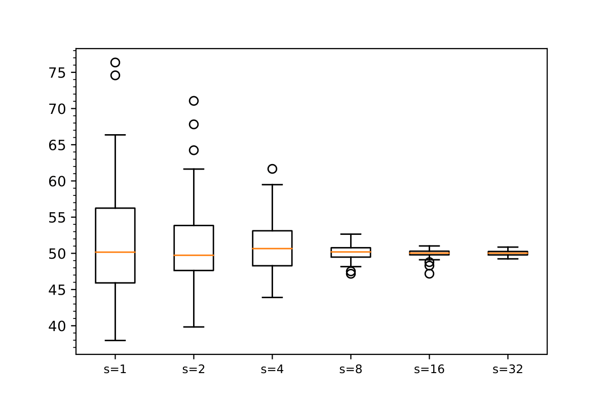
(a) Confidence Intervals for $\alpha_{1}$ (True value = 50)

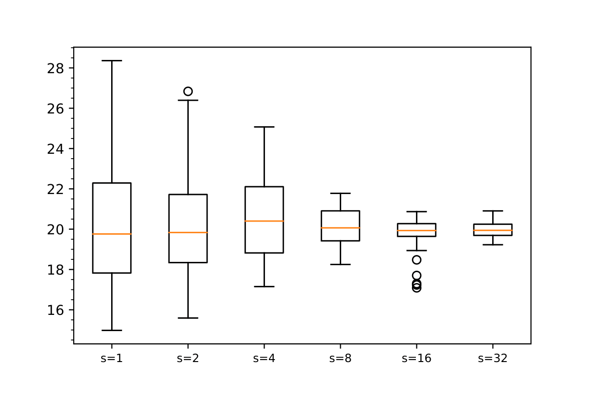
(b) Confidence Intervals for $\alpha_{2}$ (True value = 20)

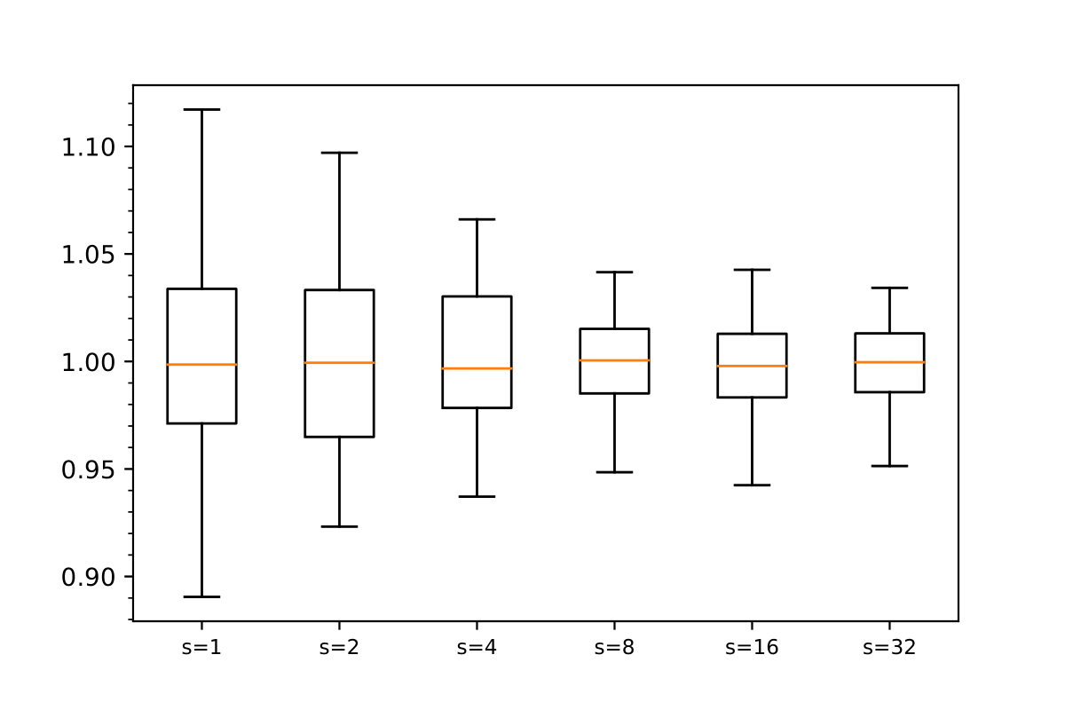
(c) Confidence Intervals for $\alpha_{3}$ (True value = 1)

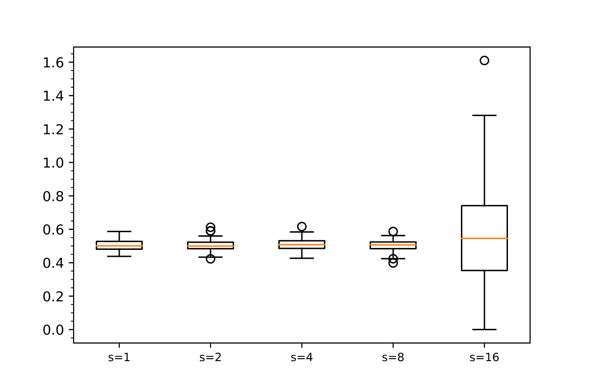
(d) Confidence Intervals for $\theta$ (True value = 0.5)

Figure 5: Box plots of Model I - Submodel 1 estimates

7.1.2 Weighted sinsuoidal arrival rate and hyperexponentially distributed patience

In this example, our model of choice is an M_t/M/$s$+H system, with arrival rate, service distribution and patience distribution given by

$$\lambda_{{\bm{\alpha}}}(t) =50+15\sin\big{(}4-0.1t\big{)}+10\sin\big{(}1-0.5t\big{)},$$

$$M \sim\text{Exp}(0.4),$$

$$H_{{\bm{\theta}}}(x) =1-0.8e^{-x}-0.2e^{-0.1x}.$$

The parameters to be estimated are therefore ${\bm{\alpha}}_{0}=(50,15,10,4,1)$, and ${\bm{\theta}}_{0}=(0.8,1,0.1)$. In this example, the number of total arrivals is $10^{6}$, leading to the box plots of Figure 6. Similar to the previous model, we observe that accuracy of the estimator of ${\bm{\alpha}}$ improves as the number of servers increases. However, the estimates corresponding to ${\bm{\theta}}$ now do not exhibit a clear pattern. When the number of servers is low (say, $s=1$), the estimates of $\theta_{3}$ is accurate, whereas the estimate of $\theta_{2}$ is poor. This is because virtual waiting times are typically high, entailing that all customers with patience sampled from the $\text{Exp}(1)$ distribution tend to get rejected due to their low patience values. Therefore, a large proportion of non-balking customers have patience sampled from $\text{Exp}(0.1)$, so that $\theta_{3}$ can be estimated accurately but $\theta_{2}$ not. This model requires a substantial amount of data for the estimation procedure for multiple reasons, one of which has been discussed in Example 1.2. The other reason is that the log-likelihood has a rather irregular surface, which is hard to optimize over (in comparison to the previous model).

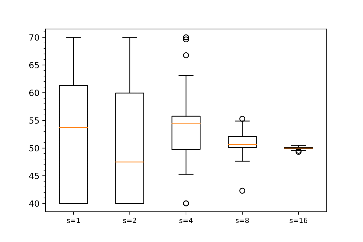
(a) Confidence Intervals for $\alpha_{1}$ (True value = 50)

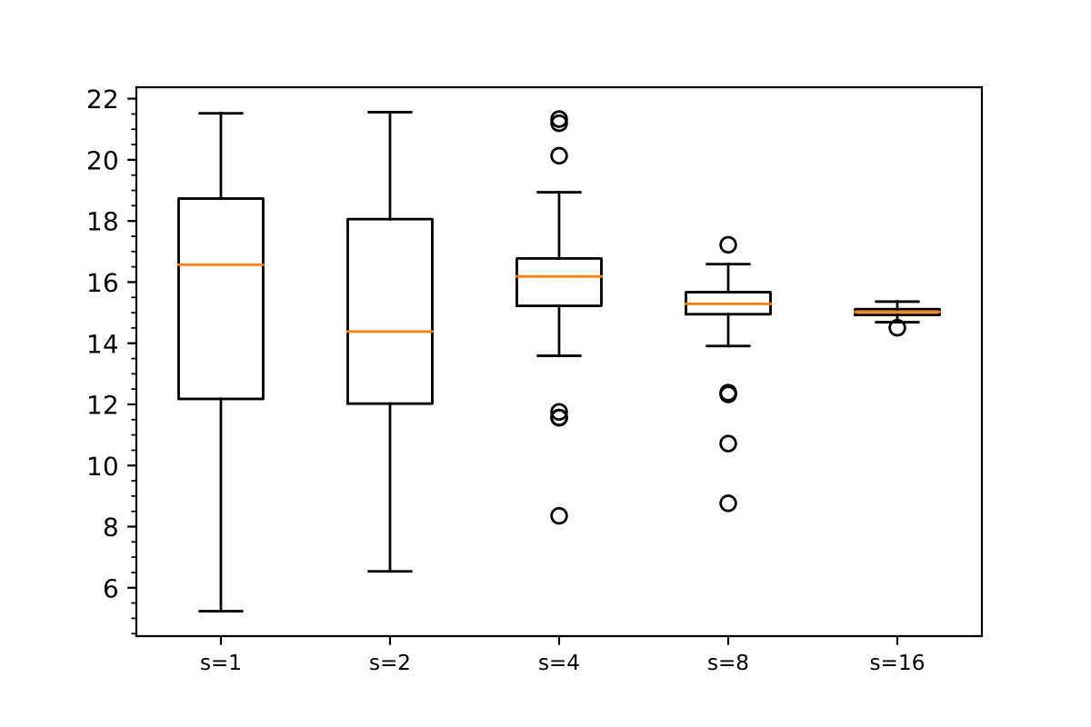
(b) Confidence Intervals for $\alpha_{2}$ (True value = 15)

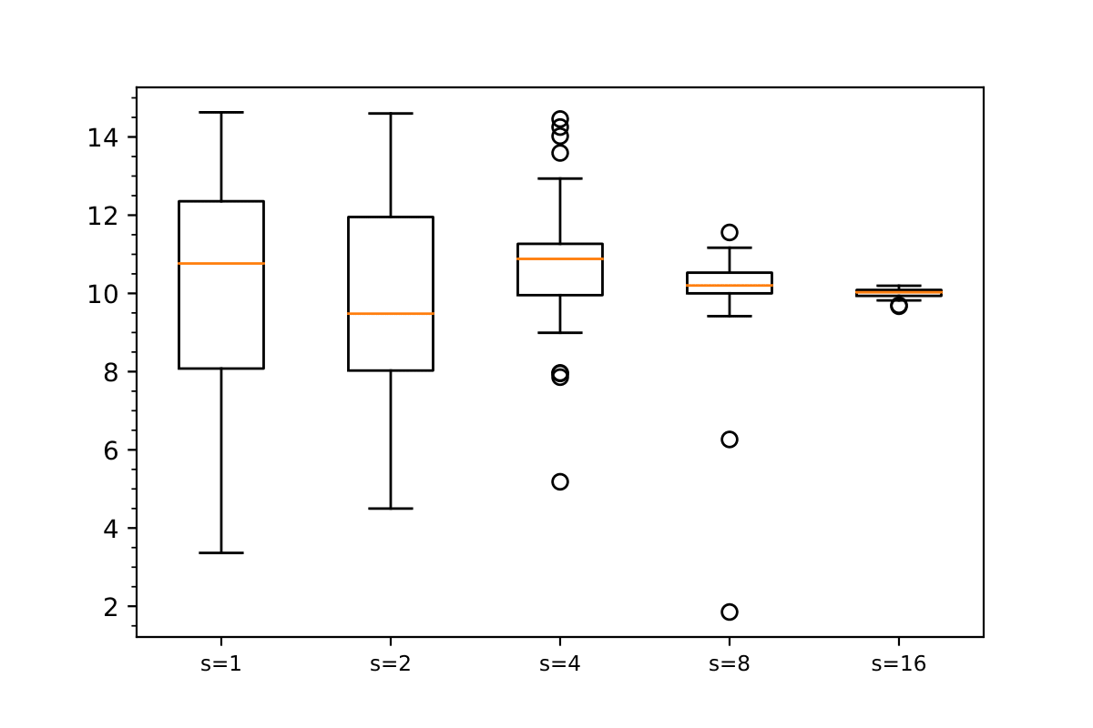
(c) Confidence Intervals for $\alpha_{3}$ (True value = 10)

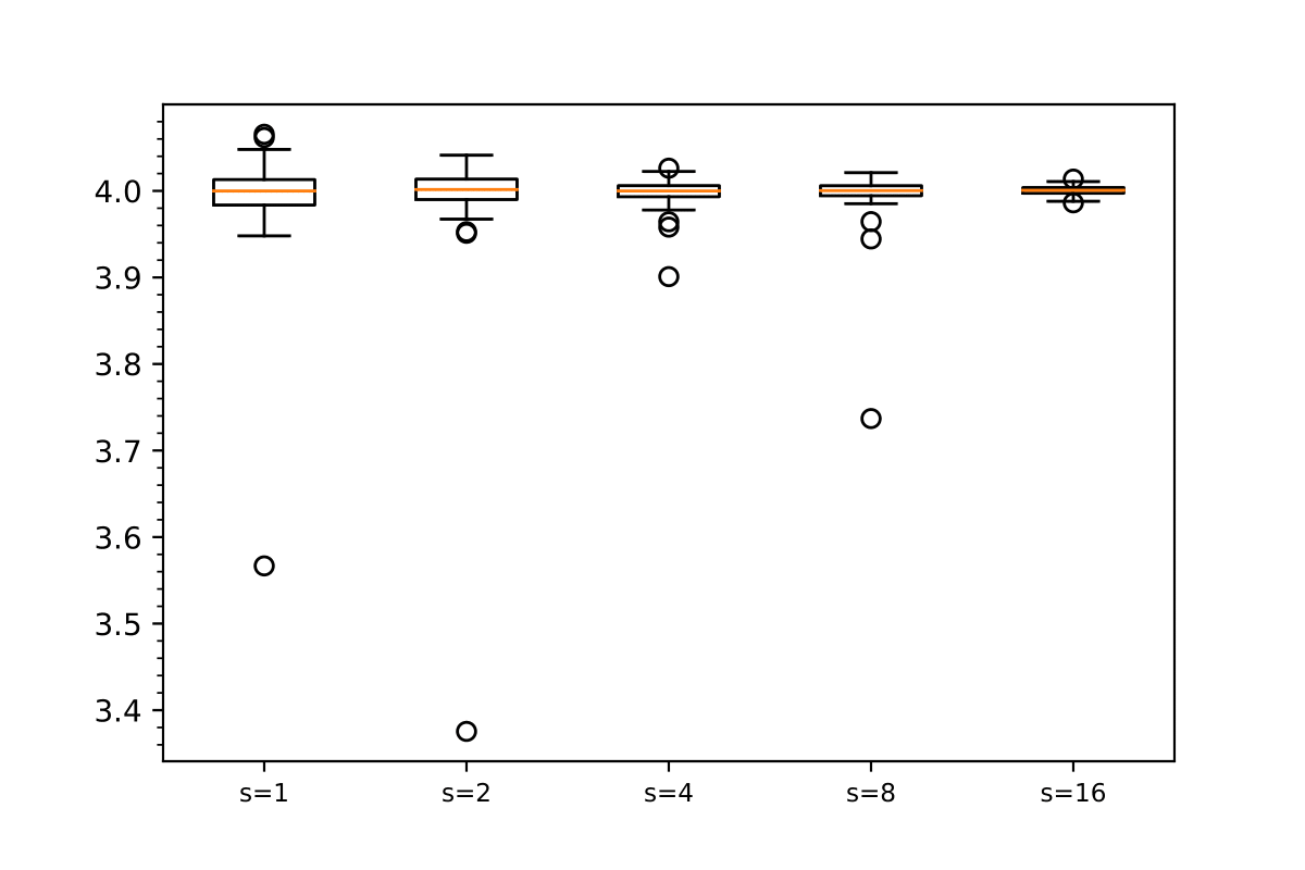
(d) Confidence Intervals for $\alpha_{4}$ (True value = 4)

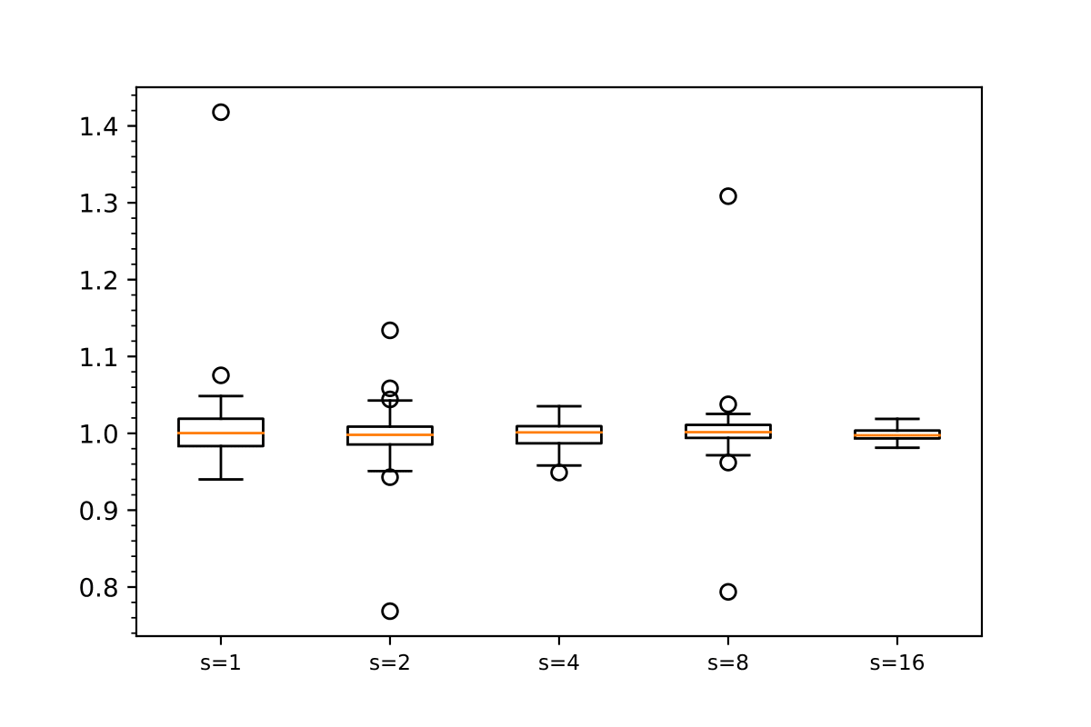
(e) Confidence Intervals for $\alpha_{5}$ (True value = 1)

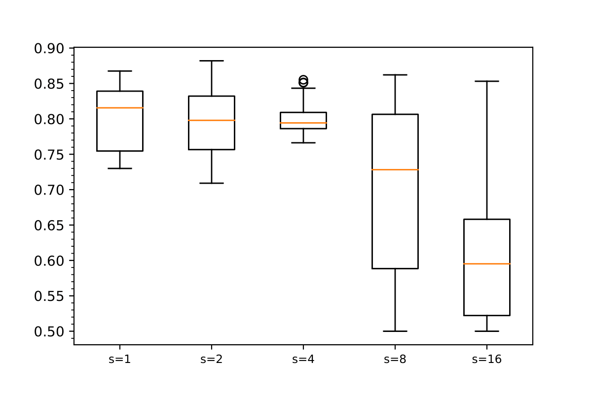
(f) Confidence Intervals for $\theta_{1}$ (True value = 0.8)

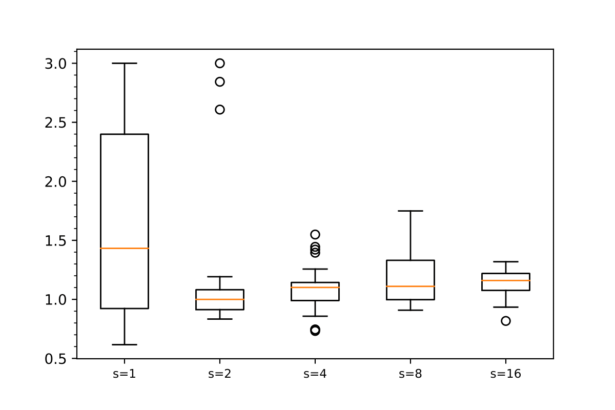
(g) Confidence Intervals for $\theta_{2}$ (True value = 1)

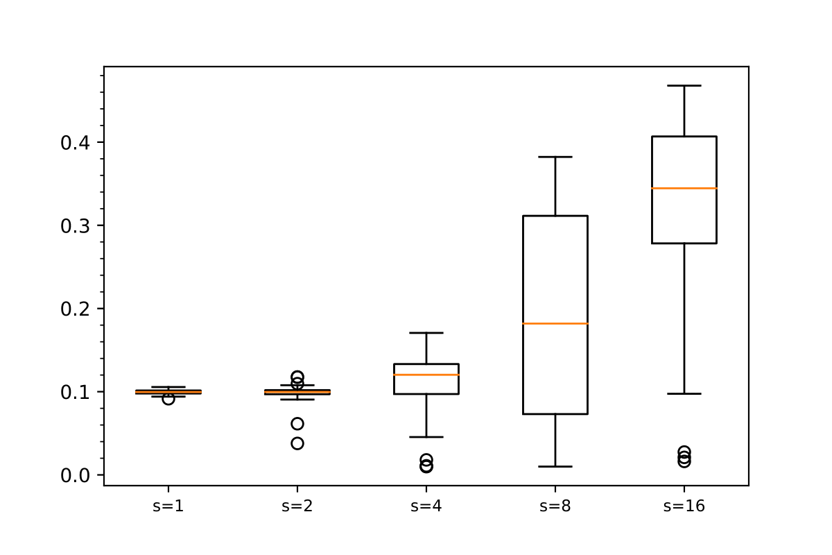
(h) Confidence Intervals for $\theta_{3}$ (True value = 0.1)

Figure 6: Box plots of Model I - Submodel 2 estimates

Model II: Estimated virtual waiting time based joining

We now demonstrate the procedure working with incomplete information, as was presented in Section 6, in which the delay proxy at time $t$ can be any estimate of the waiting time, depending only on the information in the regeneration cycle time $t$ belongs to. In this particular experiment we choose $\psi\big{(}\mathcal{R}(t)\big{)}=(L(t)-s+1)^{+}\,{\mathbb{E}}B/s$, where $L(t)=|{\mathcal{R}}(t)|$ denotes the number of customers in the system at time $t$. Our model of choice is an M_t/G/$s$+H system with arrival rate, service disribution and patience distribution given by

$$\lambda_{{\bm{\alpha}}}(t) =50+20\sin(4-0.1t)+10\sin(1-0.5t),$$

$$G \sim\text{Gamma}(0.1,4),$$

$$H_{{\bm{\theta}}}(x) =1-\frac{1}{(1+x)^{2}}.$$

The paramaters to be estimated are therefore ${\bm{\alpha}}_{0}=(50,20,10,4,1)$, and ${\bm{\theta}}_{0}=(1,2)$. We use simulated data from 0.5$\times 10^{6}$ total arrivals (balking and non-balking). Figure 7 shows the box plots for the empirical confidence intervals of the estimates for ${\bm{\alpha}}$ and ${\bm{\theta}}$. They follow a similar trend as in the one observed in previous examples.

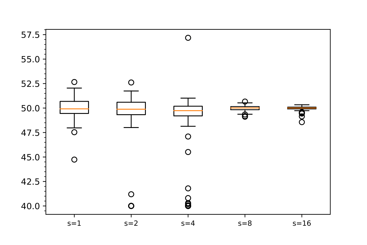
(a) Confidence Intervals for $\alpha_{1}$ (True value = 50)

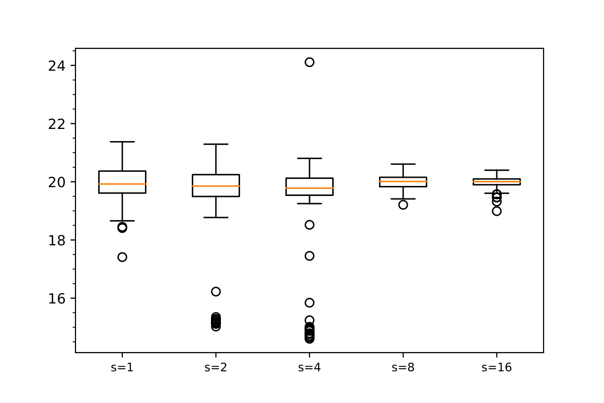
(b) Confidence Intervals for $\alpha_{2}$ (True value = 20)

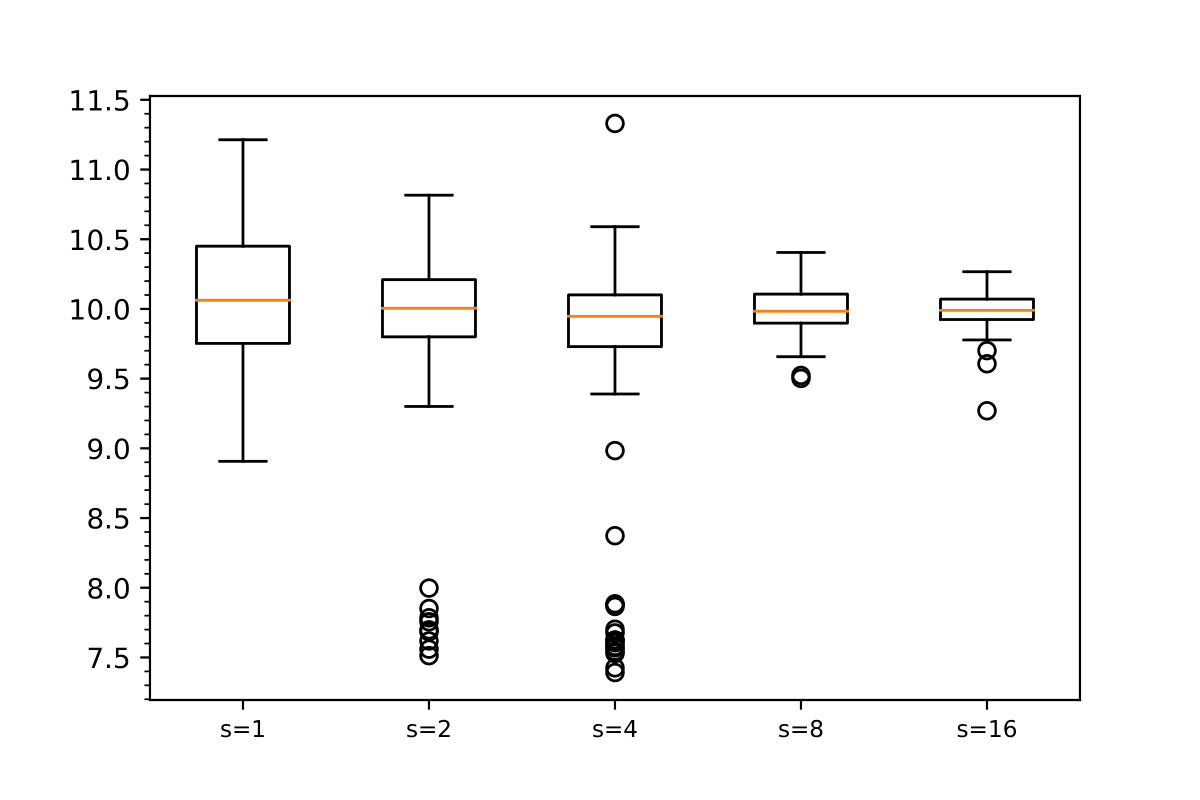
(c) Confidence Intervals for $\alpha_{3}$ (True value = 10)

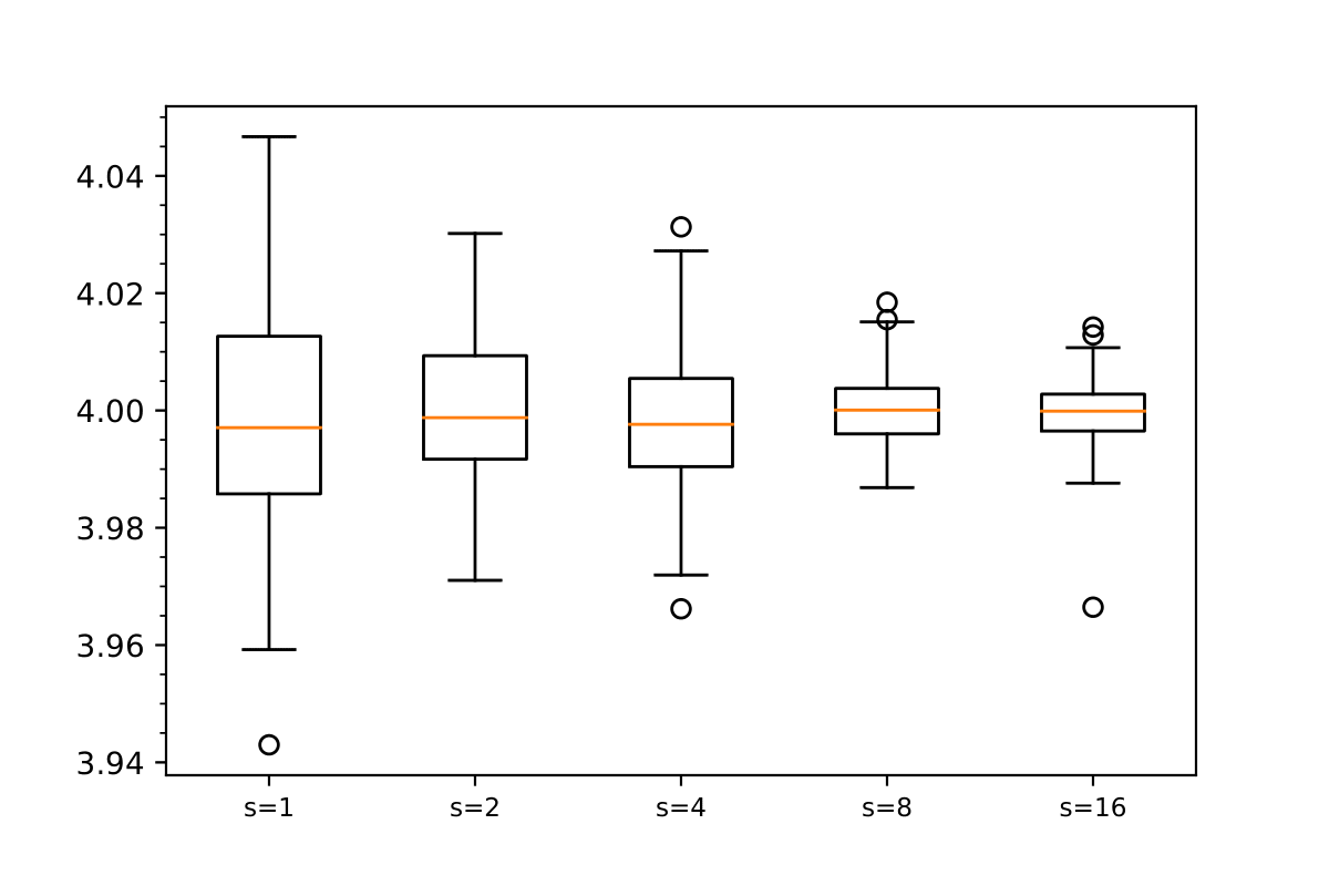
(d) Confidence Intervals for $\alpha_{4}$ (True value = 4)

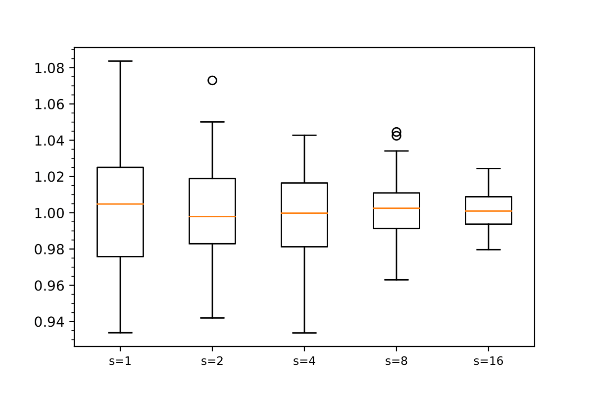
(e) Confidence Intervals for $\alpha_{5}$ (True value = 1)

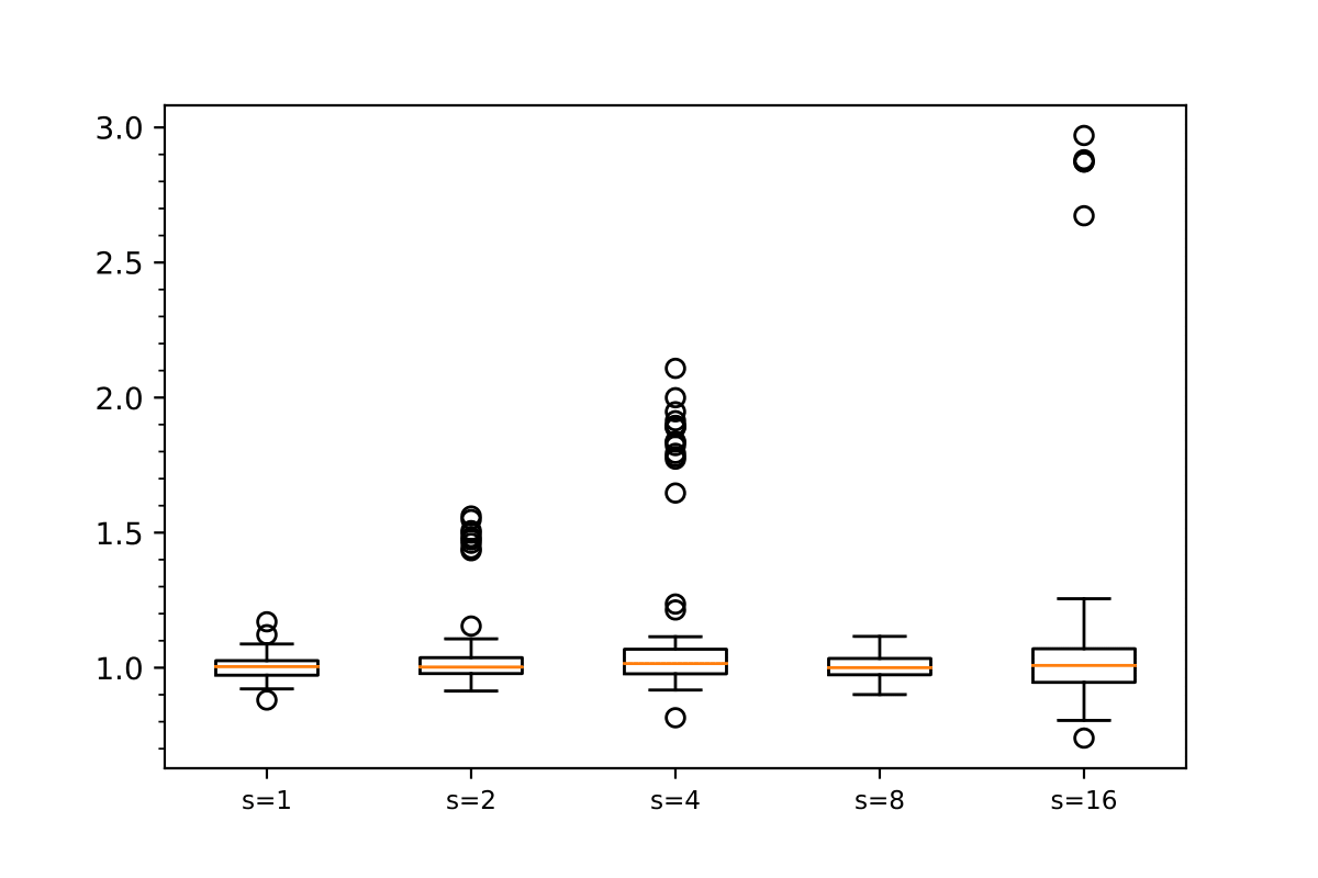
(f) Confidence Intervals for $\theta_{1}$ (True value = 1)

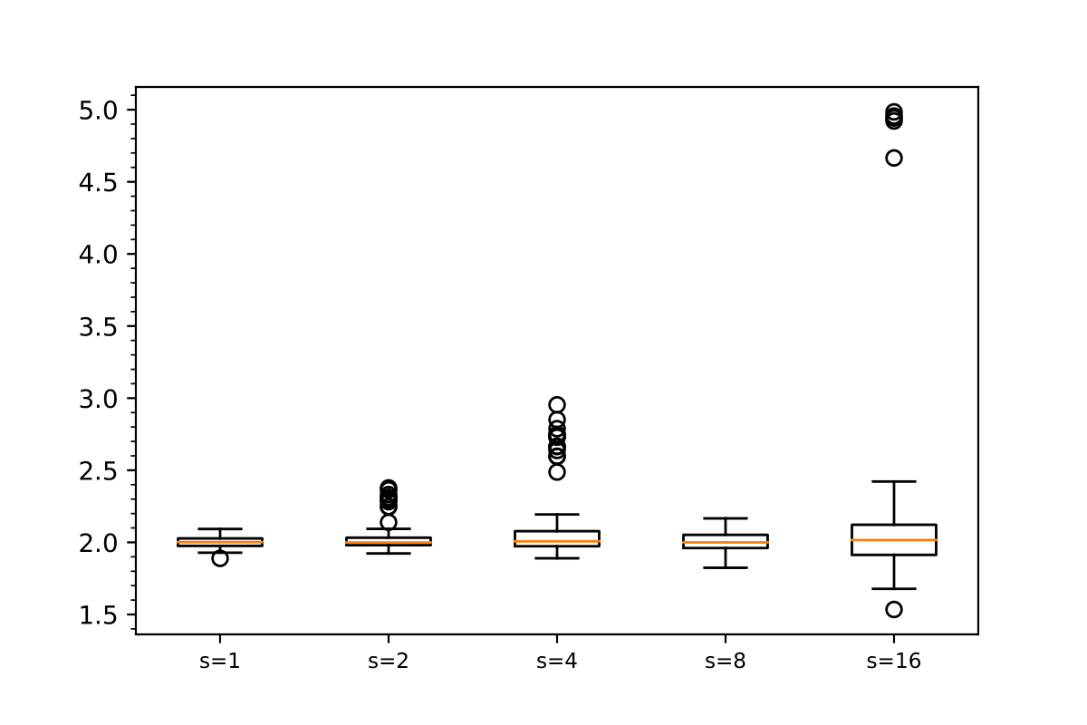
(g) Confidence Intervals for $\theta_{2}$ (True value = 2)

Figure 7: Box plots of Model II estimates

Model III: System size based joining

In this model, an arriving customer only receives information about the total number of customers in the system at time $t$, i.e. $\psi\big{(}\mathcal{R}(t)\big{)}=L(t)$. Or alternatively, an arriving customer receives information about the number of service completions that they must wait for, before their service begins. That is, $\psi\big{(}\mathcal{R}(t)\big{)}=\big{(}L(t)-s+1\big{)}^{+}$. In particular, our model of interest is an M_t/G/$s$+H system with arrival rate, service distribution and patience distribution given by

$$\lambda({\bm{\alpha}},t) =50+20\sin(4-0.1t)+10\sin(1-0.5t),$$

$$G \sim\text{Gamma}(0.05,4),$$

$$H_{{\bm{\theta}}} \sim\text{Geo}(0.1).$$

The paramaters to be estimated are therefore ${\bm{\alpha}}_{0}=(50,20,10,4,1)$, and ${\bm{\theta}}_{0}=0.1$. In this example, we work with 40,000 total arrivals. Box plots of empirical confidence intervals for the estimates of ${\bm{\alpha}}$ and ${\bm{\theta}}$ are shown in Figure 8. Once again, we observe that they follow a similar trend as in the previous examples.

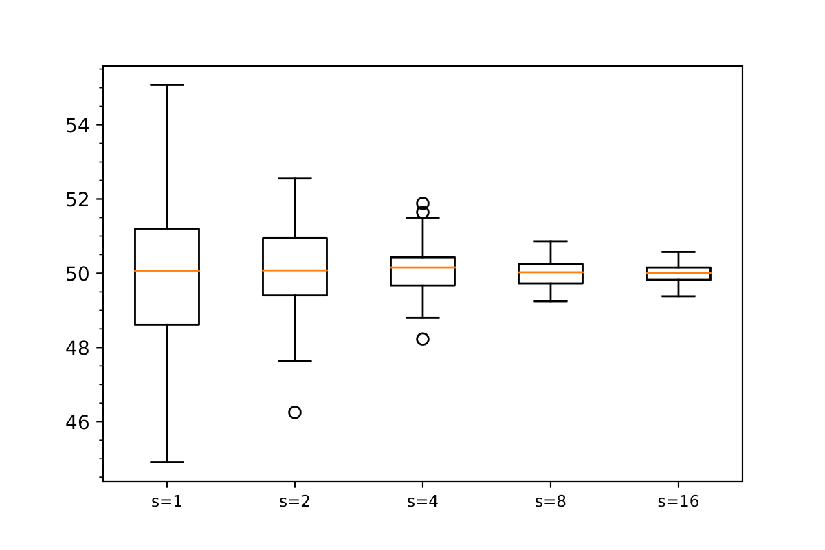
(a) Estimates for $\alpha_{1}$ (True value = 50)

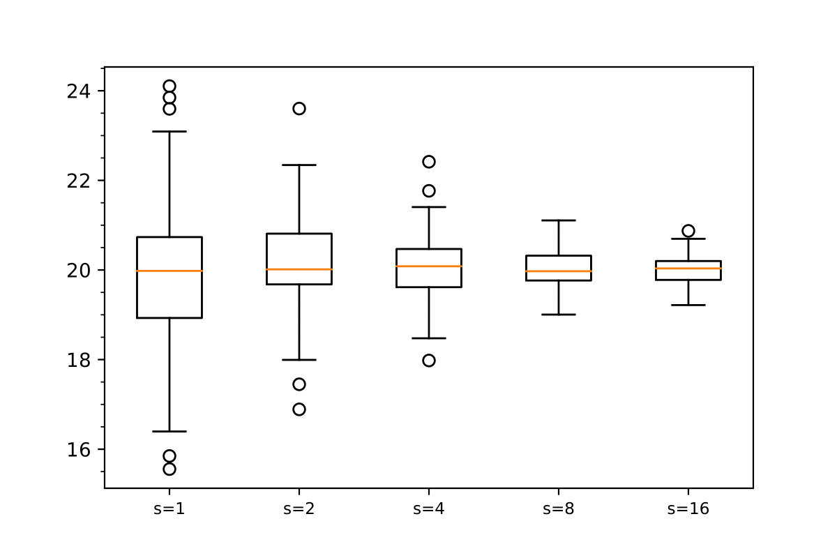
(b) Estimates for $\alpha_{2}$ (True value = 20)

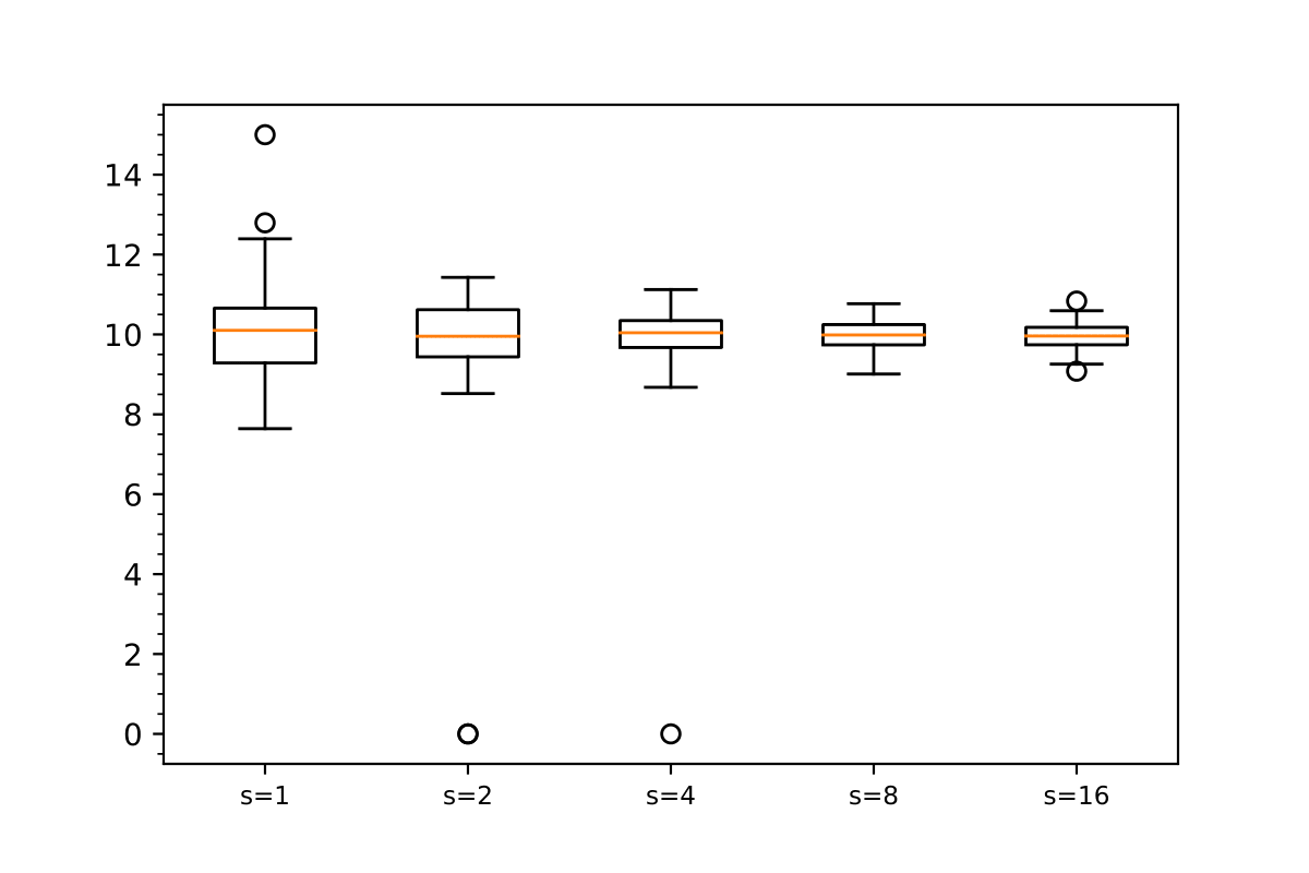
(c) Estimates for $\alpha_{3}$ (True value = 10)

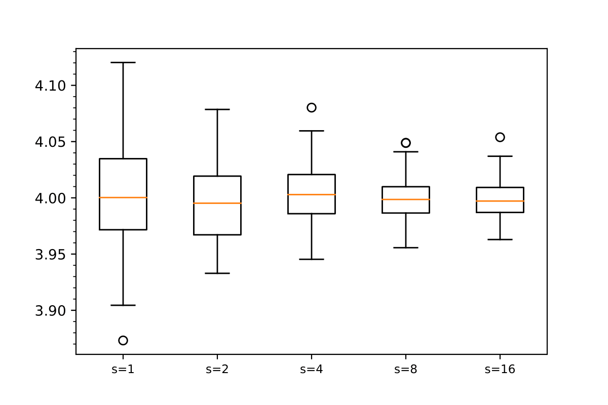
(d) Estimates for $\alpha_{4}$ (True value = 4)

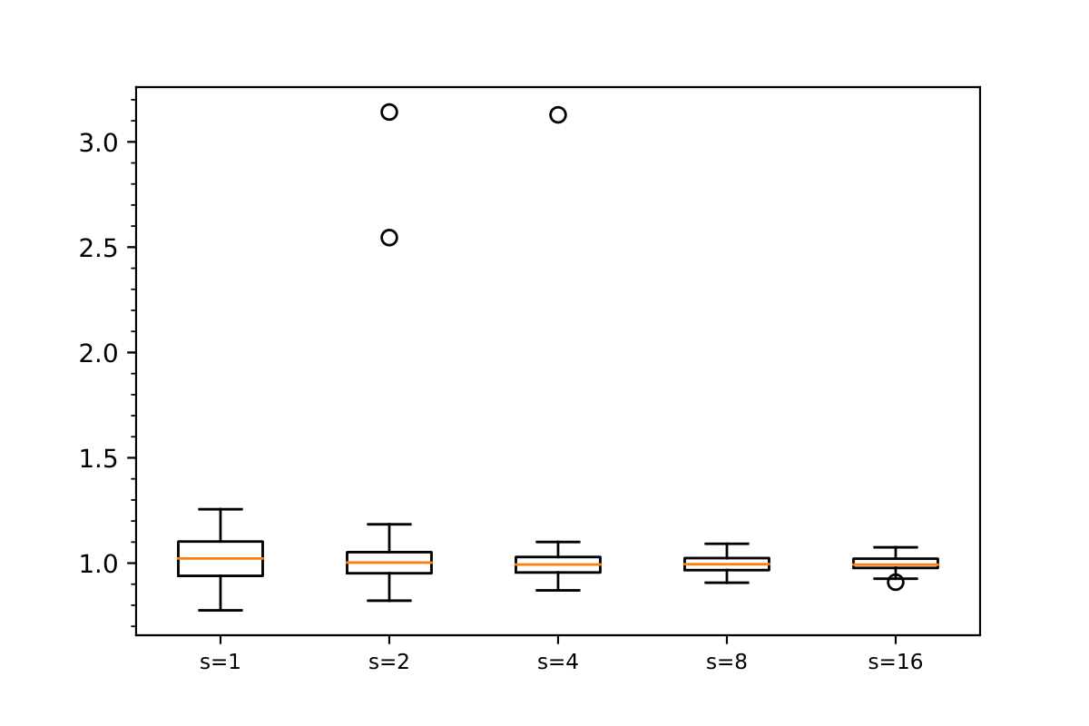
(e) Estimates for $\alpha_{5}$ (True value = 1)

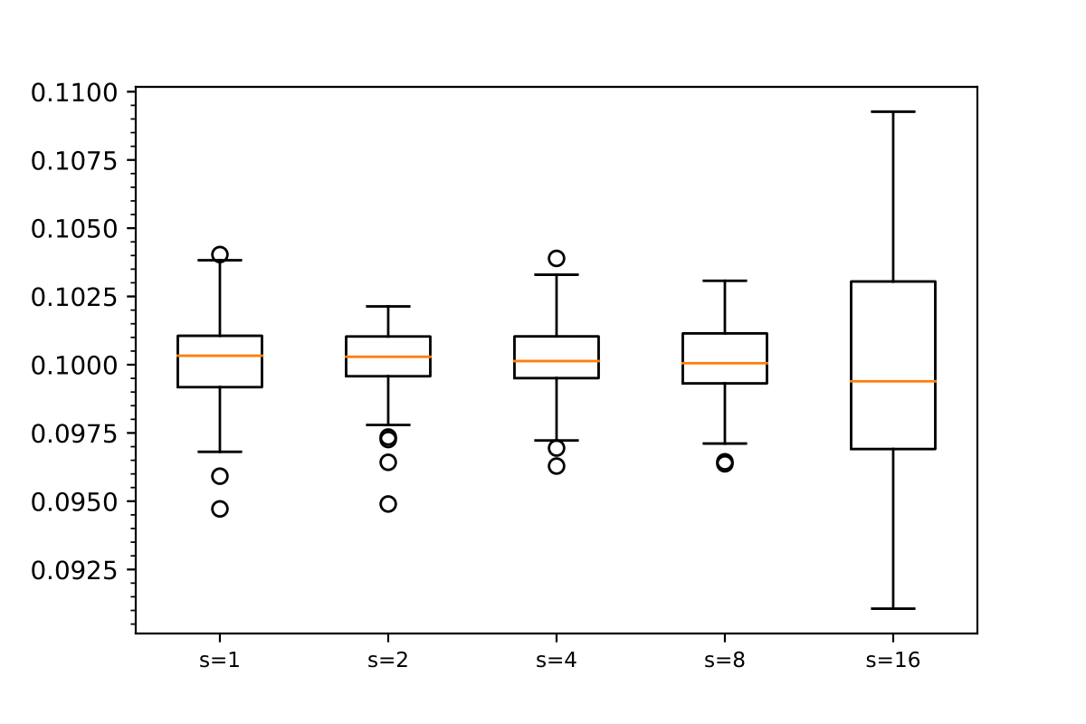
(f) Estimates for $\theta$ (True value = 0.1)

Figure 8: Box plots of Model III estimates

CONCLUDING REMARKS

In this paper, we considered a service system where arriving clients are provided information about their expected delay before joining service. Based on their patience level, customers decide to join the system or to balk. As the underlying model we chose the versatile M_t/G/$s$+H queue, with a periodic time-dependent arrival rate $\lambda_{{\bm{\alpha}}_{0}}(t)$, and a patience distribution $H_{{\bm{\theta}}_{0}}(\cdot)$. The goal of this paper was to estimate the parameter vectors ${\bm{\alpha}}_{0}$ and ${\bm{\theta}}_{0}$, even though the balking customers remain unobserved. Through an MLE procedure, we devised estimators $\hat{{\bm{\alpha}}}_{n}$ and $\hat{{\bm{\theta}}}_{n}$ given an observed realization of the system corresponding to $n$ non-balking customers, which we proved to be consistent and asymptotically normal as $n\to\infty$. Through numerical experiments, some of them working with delay proxies, we demonstrate the performance of the estimation procedure. We also illustrate instances where estimation is easier and harder, with supporting explanations for the same.

Although the framework considered is rather general, several extensions could be thought of. An interesting generalization could be one in which the service times and patience levels are correlated, which could e.g. cover cases in which a customer with a large job size is naturally willing to wait longer than customers with smaller job sizes.

In the context of our paper the impatience mechanism can be seen as a decentralized control policy, in that it makes sure that the number of customers in the system does not become large. Thus, the material presented in this work is an example of an estimation problem based on partial information, in a system that operates under what could be called an ‘equalizing control’. In the introduction of our paper we came across instances in which (some of) the parameters were hard to identify, corresponding to situations in which the control succeeded in essentially equalizing the system occupancy, entailing that relatively little information in our observations. The complications arising when aiming to estimate parameters under ‘equalizing control measures’ are discussed in detail in [30]: the control tries to make the congestion level as constant as possible, whereas estimation would benefit from more fluctuations.

ONLINE APPENDIX

Appendix A ANALYSIS OF M_t/G/$s$+H SYSTEM

In Section 4, we constructed a number of random variables pertaining to a regeneration cycle of an M_t/G/$s$+H system and then made some intuitive claims about them in Theorem 4.1. In this appendix we prove this theorem.

Proof of Theorem 4.1(a).

Let $\{{\bm{X}_{n}}\}_{n\geq 0}$ denote the vector of residual service times at times $0,1,2,\cdots$, i.e., ${\bm{X}_{n}}=\big{(}X_{n,1},X_{n,2},\cdots,X_{n,s}\big{)}\in\mathbb{R}_{+}^{s}$ where $X_{n,i}$ denotes the residual service time corresponding to server $i$ at time $n$. Then, $\{{\bm{X}_{n}}\}_{n\geq 0}$ is a discrete-time Markov chain. Also define $\{{\bm{L}_{n}}\}_{n\geq 1},\{{\bm{T}_{n}}\}_{n\geq 1}\in\mathbb{R}^{s}$ as follows: ${\bm{L}_{n}}=\big{(}L_{n,1},L_{n,2},\cdots,L_{n,s}\big{)}$ where $L_{n,i}$ denotes the amount of workload server $i$ receives during time $(n-1,n]$, and ${\bm{T}_{n}}=\big{(}T_{n,1},T_{n,2},\cdots,T_{n,s}\big{)}$ where $T_{n,i}$ denotes the amount of service completed by server $i$ during time $(n-1,n]$. If a server $i$ is never idle during $(n-1,n]$, then $T_{n,i}=1$, otherwise $T_{n,i}<1$.

By Assumption (A4), there exists $1>\delta>0$ and $p\geq 2$ such that

$$\lambda_{\max}\operatorname{\mathbb{E}}(B)\tilde{H}_{{\bm{\theta}}}(p-1)\leq 1-\delta.$$

We define the Lyapunov function $\phi:\mathbb{R}^{s}_{+}\mapsto[1,\infty)$ by

$$\phi({\bm{x}})=1+\frac{1}{\delta}\max_{i=1,2,\cdots,s}{x_{i}}.$$ (A.1)

Let $\mathcal{C}$ denote the set $[0,k]^{s}$ for $k\gg p$, the exact lower bound for $k$ being evaluated later. Suppose ${\bm{X}_{n}}\in\mathcal{C}$. Then we show that $\operatorname{\mathbb{E}}\big{[}\phi\big{(}{\bm{X}_{n+1}}\big{)}|{\bm{X}_{n}}\big{]}$ is bounded above by some fixed quantity, as follows:

$$\operatorname{\mathbb{E}}\big{[}\phi\big{(}{\bm{X}_{n+1}}\big{)}\ \big{|}{\bm{X}_{n}}\big{]} =\operatorname{\mathbb{E}}\bigg{[}1+\frac{1}{\delta}\max_{i=1,2,\cdots,s}\big{(}X_{n,i}+L_{n+1,i}-T_{n+1,i}\big{)}\ \Big{|}{\bm{X}_{n}}\bigg{]}$$

$$\leq 1+\frac{1}{\delta}\max_{i=1,2,\cdots,s}X_{n,i}+\frac{1}{\delta}\operatorname{\mathbb{E}}\Bigg{[}\sum_{i=1}^{s}L_{n+1,i}\ \Big{|}{\bm{X}_{n}}\Bigg{]}$$

$$\leq 1+\frac{k}{\delta}+\frac{\lambda_{\max}\operatorname{\mathbb{E}}(B)}{\delta}.$$ (A.2)

Suppose now that ${\bm{X}_{n}}\in\mathbb{R}^{s}\setminus\mathcal{C}$. Then, we consider two distinct cases as follows.

Case I: $\min_{i=1,2,\cdots,s}X_{n,i}\geq p$

In this case,

$$\operatorname{\mathbb{E}}\big{[}\phi\big{(}{\bm{X}_{n+1}}\big{)}-\phi\big{(}{\bm{X}_{n}})\ \big{|}{\bm{X}_{n}}\big{]} =\ \operatorname{\mathbb{E}}\bigg{[}\cancel{1}+\frac{1}{\delta}\max_{i=1,2,\cdots,s}\big{(}X_{n,i}+L_{n+1,i}-1\big{)}-\cancel{1}-\frac{1}{\delta}\max_{i=1,2,\cdots,s}X_{n,i}\ \Big{|}{\bm{X}_{n}}\bigg{]}$$

$$\leq\ \frac{1}{\delta}\operatorname{\mathbb{E}}\bigg{[}\cancel{\max_{i=1,2,\cdots,s}X_{n,i}}+\max_{i=1,2,\cdots,s}L_{n+1,i}-1-\cancel{\max_{i=1,2,\cdots,s}X_{n,i}}\ \Big{|}{\bm{X}_{n}}\bigg{]}$$

$$\leq\ \frac{1}{\delta}\bigg{(}-1+\operatorname{\mathbb{E}}\bigg{[}\sum_{i=1}^{s}L_{n+1,i}\ \Big{|}{\bm{X}_{n}}\bigg{]}\bigg{)}$$

$$\leq\ \frac{1}{\delta}\Big{(}-1+\lambda_{\max}\operatorname{\mathbb{E}}(B)\tilde{H}_{\theta}(p-1)\Big{)}$$

$$\leq\ \frac{1}{\delta}\big{(}-1+1-\delta\big{)}=-1.$$ (A.3)

Case II: $\min_{i=1,2,\cdots,s}X_{n,i}<p$

Denote the total incoming workload during the interval $(n,n+1]$ by $W_{(n,n+1]}$. Then,

$$\operatorname{\mathbb{E}}\big{[}\phi ({\bm{X}_{n+1}})-\phi({\bm{X}_{n}})|{\bm{X}_{n}}\big{]}$$

$$=\ -\frac{1}{\delta}\operatorname{\mathbb{P}}\Big{(}W_{(n,n+1]}\leq k-p-1\Big{)}+\operatorname{\mathbb{E}}\Big{[}\big{(}\phi({\bm{X}_{n+1}})-\phi({\bm{X}_{n}})\big{)}\operatorname{\mathbb{I}}\Big{(}W_{(n,n+1]}>k-p-1\Big{)}\ \big{|}{\bm{X}_{n}}\Big{]}.$$ (A.4)

Explanation for the first term of (A.4): During the time interval $(n,n+1]$, the difference between the workloads of maximum and minimum workload servers is at least $k-p-1$. Therefore, if $W_{(n,n+1]}<k-p-1$, then it will always be assigned to some server which is not the maximum workload server. In this case, $\phi({\bm{X}_{n+1}})-\phi({\bm{X}_{n}})=-1/\delta$. The second term of (A.4) is majorized by

$$\operatorname{\mathbb{E}}\Big{[}\big{(}\phi ({\bm{X}_{n+1}})-\phi({\bm{X}_{n}})\big{)}\operatorname{\mathbb{I}}\Big{(}W_{(n,n+1]}>k-p-1\Big{)}\ \big{|}{\bm{X}_{n}}\Big{]}$$

$$\leq\ \sum_{j=1}^{\infty}\frac{j}{\delta}\ \operatorname{\mathbb{P}}\Big{(}W_{(n,n+1]}\in\big{(}k-p+j-2,\ k-p+j-1\big{)}\ \big{|}{\bm{X}_{n}}\Big{)}$$

$$\leq\ \frac{1}{\delta}\int_{k-p-1}^{\infty}(x-k+p+2)\ f_{W_{(n,n+1]}|{\bm{X}_{n}}}(x)\ \mathrm{d}x$$

$$\leq\ \frac{1}{\delta}\int_{k-p-1}^{\infty}x\ f_{W_{(n,n+1]}|{\bm{X}_{n}}}(x)\ \mathrm{d}x\longrightarrow 0$$

as $k\rightarrow\infty$, because $\operatorname{\mathbb{E}}\big{[}W_{(n,n+1]}\ |{\bm{X}_{n}}\big{]}\leq\lambda_{\max}\operatorname{\mathbb{E}}[B]<\infty$. Therefore, we obtain

$$\lim_{k\rightarrow\infty}\operatorname{\mathbb{E}}\Big{[}\big{(}\phi({\bm{X}_{n+1}})-\phi({\bm{X}_{n}})\big{)}\operatorname{\mathbb{I}}\Big{(}W_{(n,n+1]}>k-p-1\Big{)}\Big{]}\leq 0.$$

Since $\operatorname{\mathbb{P}}\big{(}W_{(n,n+1]}\leq k-p-1\big{)}\rightarrow 1$ as $k\rightarrow\infty$, we can conclude that

$$-\frac{1}{\delta}\operatorname{\mathbb{P}}\Big{(}W_{(n,n+1]}\leq k-p-1\Big{)}+\operatorname{\mathbb{E}}\Big{[}\big{(}\phi({\bm{X}_{n+1}})-\phi({\bm{X}_{n}})\big{)}\operatorname{\mathbb{I}}\Big{(}W_{(n,n+1]}>k-p-1\Big{)}\Big{]}\rightarrow-\frac{1}{\delta}$$

as $k\rightarrow\infty$. Since $-1/\delta<-1$, there must exist $\widetilde{k}\in\mathbb{R}$ such that the above expression is less than $-1$. Choosing $\mathcal{C}=\big{[}0,\widetilde{k}\big{]}^{s}$, we have verified that for all ${\bm{X}_{n}}\in\mathbb{R}^{s}\setminus\mathcal{C}$,

$$\operatorname{\mathbb{E}}\big{[}\phi\big{(}{\bm{X}_{n+1}}\big{)}-\phi\big{(}{\bm{X}_{n}}\big{)}\ \big{|}{\bm{X}_{n}}]\leq-1.$$

Therefore, by [4, Proposition 6.11(a)], $\mathcal{C}$ is a recurrent set. Now, let $\mathcal{U}=\{(0,0,\cdots,0)\}$. Define the induced chain $\{{\bm{Y}_{n}}\}_{n\geq 1}$ as follows:

$${\bm{Y}_{n}}={\bm{X}_{\tau_{\mathcal{C}}^{(n)}}}.$$

Choose $N=\widetilde{k}+1$, and ${\bm{Y}_{0}}={\bm{X}_{0}}=(0,0,\cdots,0)$. ${\bm{Y}_{1}}\in\mathcal{C}$ implies that $\max_{i=1,2,\cdots,s}Y_{1,i}\leq\widetilde{k}$. Under the scenario that no customers arrive for the next $\widetilde{k}$ units of time, every server’s workload continues dropping at unit rate and therefore, there exists $i\in\{2,3,\cdots,\widetilde{k}+1\}$ such that ${\bm{Y}_{i}}=(0,0,\cdots,0)$. The probability of this event is

$$\operatorname{\mathbb{P}}\Big{(}\text{No arrivals during}\ \big{(}\tau_{\mathcal{C}}^{(1)},\tau_{\mathcal{C}}^{(1)}+\widetilde{k}\big{)}\Big{)}\geq e^{-\lambda_{\max}\widetilde{k}}.$$

By [4, Proposition 6.15(i)], we get that $\mathcal{U}$ is recurrent. Furthermore, by [4, Proposition 6.15(ii)], $\sup_{x\in\mathcal{C}}\operatorname{\mathbb{E}}_{x}\big{[}\tau_{\mathcal{U}}\big{]}<\infty$. Therefore, the expected return time to $(0,0,\cdots,0)$ starting at $(0,0,\cdots,0)$ itself, is finite, i.e. $\operatorname{\mathbb{E}}(R_{1})<\infty$. ∎

Proof of Theorem 4.1(b).

The maximum amount of service that can be completed in regeneration cycle $1$ is bounded from above by $sR_{1}$, which corresponds to the scenario that each server works for the entire duration of the regeneration cycle. On the other hand, the desired amount of service is given by $B_{1,1}+B_{1,2}+\cdots+B_{1,C_{1}}$. This implies that $sR_{1}\geq B_{1,1}+B_{1,2}+\cdots+B_{1,C_{1}}$. Taking expectation on both sides and making use of the previous result, we conclude that

$$\operatorname{\mathbb{E}}\Bigg{[}\sum_{i=1}^{C_{1}}B_{1,i}\Bigg{]}<s\operatorname{\mathbb{E}}\big{[}R_{1}\big{]}<\infty.$$ (A.5)

For $k\geq 1$, define $S_{k}:=B_{1,1}+B_{1,2}+\cdots+B_{1,k}$. Then,

$$\underbrace{\sum_{i=1}^{C_{1}}B_{1,i}}_{Z}=\sum_{k=1}^{\infty}S_{k}\operatorname{\mathbb{I}}\big{\{}C_{1}=k\big{\}}=\lim_{K\rightarrow\infty}\ \underbrace{\sum_{k=1}^{K}S_{k}\operatorname{\mathbb{I}}\big{\{}C_{1}=k\big{\}}}_{Z_{K}}.$$

$0\leq Z_{1}\leq Z_{2}\leq\cdots\leq Z$ and $\lim_{K\rightarrow\infty}Z_{K}=Z$. Therefore, by the monotone convergence theorem,

$$\operatorname{\mathbb{E}} \Bigg{[}\sum_{i=1}^{C_{1}}B_{1,i}\Bigg{]}=\lim_{K\rightarrow\infty}\operatorname{\mathbb{E}}\Bigg{[}\sum_{k=1}^{K}S_{k}\operatorname{\mathbb{I}}\big{\{}C_{1}=k\big{\}}\Bigg{]}=\lim_{K\rightarrow\infty}\sum_{k=1}^{K}\operatorname{\mathbb{E}}\Big{[}S_{k}\operatorname{\mathbb{I}}\big{\{}C_{1}=k\big{\}}\Big{]}=\sum_{k=1}^{\infty}\operatorname{\mathbb{E}}\Big{[}S_{k}\operatorname{\mathbb{I}}\big{\{}C_{1}=k\big{\}}\Big{]}$$

$$=\sum_{k=1}^{\infty}\operatorname{\mathbb{E}}\Bigg{[}\sum_{i=1}^{k}B_{1,i}\operatorname{\mathbb{I}}\big{\{}C_{1}=k\big{\}}\Bigg{]}=\sum_{k=1}^{\infty}\sum_{i=1}^{k}\operatorname{\mathbb{E}}\Big{[}B_{1,i}\operatorname{\mathbb{I}}\big{\{}C_{1}=k\big{\}}\Big{]}\overset{\text{(i)}}{=}\sum_{i=1}^{\infty}\sum_{k=i}^{\infty}\operatorname{\mathbb{E}}\Big{[}B_{1,i}\operatorname{\mathbb{I}}\big{\{}C_{1}=k\big{\}}\Big{]}$$

$$=\sum_{i=1}^{\infty}\lim_{K\rightarrow\infty}\sum_{k=i}^{i+K}\operatorname{\mathbb{E}}\Big{[}B_{1,i}\operatorname{\mathbb{I}}\big{\{}C_{1}=k\big{\}}\Big{]}=\sum_{i=1}^{\infty}\lim_{K\rightarrow\infty}\operatorname{\mathbb{E}}\Bigg{[}\sum_{k=i}^{i+K}B_{1,i}\operatorname{\mathbb{I}}\big{\{}C_{1}=k\big{\}}\Bigg{]}$$

$$=\sum_{i=1}^{\infty}\lim_{K\rightarrow\infty}\operatorname{\mathbb{E}}\Big{[}B_{1,i}\operatorname{\mathbb{I}}\big{\{}i\leq C_{1}\leq i+K\big{\}}\Big{]}$$

$$\overset{\text{(ii)}}{=}\sum_{i=1}^{\infty}\operatorname{\mathbb{E}}\bigg{[}\lim_{K\rightarrow\infty}B_{1,i}\operatorname{\mathbb{I}}\big{\{}i\leq C_{1}\leq i+K\big{\}}\bigg{]}=\sum_{i=1}^{\infty}\operatorname{\mathbb{E}}\Big{[}B_{1,i}\operatorname{\mathbb{I}}\big{\{}C_{1}\geq i\big{\}}\Big{]}$$

$$\overset{\text{(iii)}}{=}\sum_{i=1}^{\infty}\operatorname{\mathbb{E}}\big{[}B_{1,i}\big{]}\operatorname{\mathbb{P}}\big{(}C_{1}\geq i\big{)}=\operatorname{\mathbb{E}}\big{[}B_{1,1}]\operatorname{\mathbb{E}}\big{[}C_{1}\big{]}.$$

The equalities in the above display are justified as follows: (i) is allowed since all summands are positive and the summation is finite; (ii) again follows because of monotone convergence theorem; (iii) holds because the event $\big{\{}C_{1}<i\big{\}}$ is independent of the random variable $B_{1,i}$. Note that $\big{\{}C_{1}<i\big{\}}$ depends on the arrival times, job sizes and patience levels pertaining to all balking and non-balking customers arriving until the $(i-1)$-st non-balking customer enters the system. It also depends on the arrival times and patience levels of subsequent customers, but not on their job sizes. In conclusion, we get

$$\operatorname{\mathbb{E}}\Bigg{[}\sum_{i=1}^{C_{1}}B_{j,i}\Bigg{]}=\operatorname{\mathbb{E}}\big{[}B_{1,1}\big{]}\operatorname{\mathbb{E}}\big{[}C_{1}\big{]}<\infty,$$

so that $\operatorname{\mathbb{E}}\big{[}C_{1}\big{]}<\infty$. ∎

Proof of Theorem 4.1(c).

Let $\{t_{n}:n\geq 0\}$, $\{a_{n}:n\geq 0\}$ be defined as follows: $t_{0}=0$, and for $k\geq 0$,

$$a_{k} =\text{Number of effective arrivals during }(0,t_{k}],$$

$$t_{k+1} =\min\Big{\{}\big{\lceil}t_{k}+\big{\rceil},\tilde{A}_{a_{k}+1}\Big{\}}.$$

Consider the process $\big{\{}Y_{n}:n\geq 0\big{\}}$ given by $Y_{n}=\big{\{}t_{n},{\bm{X}(t_{n})}\big{\}}$ where ${\bm{X}(t_{n})}$ is the vector of residual service times at time $t_{n}$, i.e., ${\bm{X}}(t_{n})\in\mathbb{R}^{s}$ stores the amount of residual workload corresponding to each of the $s$ servers. The evolution of this process can be described as a join-the-shortest workload system (which for the purposes here is identical to our system). Intuitively, the process $\big{\{}Y_{n}:n\geq 0\big{\}}$ captures the pending workload for each server after every effective arrival and at integral time points. Define

$$\tau=\inf\Big{\{}k\in\mathbb{N}\>\big{|}\ t_{k}\in\mathbb{N}\ \text{and}\ {\bm{X}(t_{k})}={\bm{0}}_{s\times 1}\Big{\}}.$$

Then, the process $\{Y_{n}:n\geq 0\}$ regenerates at time $\tau$. Define a mapping

$$f({\bm{Y}_{j}})=\min_{i=1,2,\cdots,s}X_{i}(t_{j}).$$

By the renewal-reward theorem, we get

$$\lim_{n\rightarrow\infty}\ \frac{1}{n}\sum_{j=1}^{n}f({\bm{Y}_{j}})=\frac{1}{\operatorname{\mathbb{E}}\tau}\operatorname{\mathbb{E}}\Bigg{[}\sum_{j=0}^{\tau-1}f({\bm{Y}_{j}})\Bigg{]}.$$ (A.6)

By the ergodic theorem, the LHS of (A.6) is finite almost surely. Furthermore, $\operatorname{\mathbb{E}}[\tau]<\infty$. Therefore,

$$\operatorname{\mathbb{E}}\Bigg{[}\sum_{j=0}^{\tau-1}f({\bm{Y}_{j}})\Bigg{]}<\infty.$$

The above quantity represents the expected sum of virtual waiting times just after arrival instants as well as at integral time points, which is greater than the sum of virtual waiting times just before effective arrival instants. This implies that

$$\operatorname{\mathbb{E}}\Bigg{[}\sum_{i=1}^{C_{1}}W_{1,i}\Bigg{]}\leq\operatorname{\mathbb{E}}\Bigg{[}\sum_{j=0}^{\tau-1}f({\bm{Y}_{j}})\Bigg{]}<\infty.$$

Hence we conclude that the expected sum of waiting times of customers in a regeneration cycle is finite. ∎

Appendix B PROOFS OF AUXILIARY RESULTS

Proof for Lemma 5.1 in Section 5.

By the triangle inequality, we can write

$$\Big{|}q\big{(}{\bm{Z}_{j}},{\bm{\mu}^{\prime}}\big{)}-q\big{(}{\bm{Z}_{j}},{\bm{\mu}}\big{)}\Big{|}\leq\sum_{i=1}^{C_{j}}\underbrace{\Big{|}\log\lambda_{{\bm{\alpha}}^{\prime}}\big{(}\tilde{A}_{j,i}\big{)}-\log\lambda_{{\bm{\alpha}}}\big{(}\tilde{A}_{j,i}\big{)}\Big{|}}_{\text{(I)}}+\int_{0}^{A_{j,1}}\underbrace{\Big{|}\lambda_{{\bm{\alpha}}^{\prime}}(u)-\lambda_{{\bm{\alpha}}}(u)\Big{|}}_{\text{(II)}}\,\mathrm{d}u\ +$$

$$\sum_{i=2}^{C_{j}}\underbrace{\Big{|}\log\tilde{H}_{{\bm{\theta}^{\prime}}}\big{(}W_{j,i-1}+X_{j,i-1}-A_{j,i}\big{)}-\log\tilde{H}_{{\bm{\theta}}}\big{(}W_{j,i-1}+X_{j,i-1}-A_{j,i}\big{)}\Big{|}}_{\text{(III)}}\ +$$

$$\sum_{i=2}^{C_{j}}\int_{0}^{A_{j,i}}\underbrace{\Big{|}\lambda_{{\bm{\alpha}}^{\prime}}\big{(}u+\tilde{A}_{j,i-1}\big{)}\tilde{H}_{{\bm{\theta}^{\prime}}}\big{(}W_{j,i-1}+X_{j,i-1}-u\big{)}-\lambda_{{\bm{\alpha}}}\big{(}u+\tilde{A}_{j,i-1}\big{)}\tilde{H}_{{\bm{\theta}}}\big{(}W_{j,i-1}+X_{j,i-1}-u\big{)}\Big{|}}_{\text{(IV)}}\,\mathrm{d}u\,+$$

$$\int_{0}^{R_{j}-\tilde{A}_{j,C_{j}}}\underbrace{\Big{|}\lambda_{{\bm{\alpha}}^{\prime}}\big{(}u+\tilde{A}_{j,C_{j}}\big{)}\tilde{H}_{{\bm{\theta}^{\prime}}}\big{(}W_{j,C_{j}}+X_{j,C_{j}}-u\big{)}-\lambda_{{\bm{\alpha}}}\big{(}u+\tilde{A}_{j,C_{j}}\big{)}\tilde{H}_{{\bm{\theta}}}\big{(}W_{j,C_{j}}+X_{j,C_{j}}-u\big{)}\Big{|}}_{\text{(V)}}\,\mathrm{d}u.$$ (B.1)

Let us analyze (I), (II), (III), (IV), (V) separately. Upper bounds for (I) and (II) follow from Assumption (A3) and its corresponding discussion, the upper bound for (III) follows due to (A6), and upper bounds for (IV) and (V) follow due to (A2), (A3) and (A5). Concretely,

(I): $$\Big{|}\log\lambda_{{\bm{\alpha}}^{\prime}}\big{(}\tilde{A}_{j,i}\big{)}-\log\lambda_{{\bm{\alpha}}}\big{(}\tilde{A}_{j,i}\big{)}\Big{|}\leq\frac{\kappa}{\lambda_{\min}}\ d\big{(}{\bm{\alpha}}^{\prime},{\bm{\alpha}}\big{)}.$$

(II): $$\Big{|}\lambda_{{\bm{\alpha}}^{\prime}}(u)-\lambda_{{\bm{\alpha}}}(u)\Big{|}\leq\kappa\ d\big{(}{\bm{\alpha}}^{\prime},{\bm{\alpha}}\big{)}.$$

(III): $$\Big{|}\log\tilde{H}_{{\bm{\theta}^{\prime}}}\big{(}W_{j,i-1}+X_{j,i-1}-A_{j,i}\big{)}-\log\tilde{H}_{{\bm{\theta}}}\big{(}W_{j,i-1}+X_{j,i-1}-A_{j,i}\big{)}\Big{|}$$

$$\leq\ G_{2}\big{(}W_{j,i-1}+X_{j,i-1}-A_{j,i}\big{)}\ d\big{(}{\bm{\theta}},{\bm{\theta}^{\prime}}\big{)}\leq G_{2}\big{(}W_{j,i}\big{)}\ d\big{(}{\bm{\theta}},{\bm{\theta}^{\prime}}\big{)}.$$

(IV): $$\Big{|}\lambda_{{\bm{\alpha}}^{\prime}}\big{(}u+\tilde{A}_{j,i-1})\tilde{H}_{{\bm{\theta}^{\prime}}}\big{(}W_{j,i-1}+X_{j,i-1}-u\big{)}-\lambda_{{\bm{\alpha}}}\big{(}u+\tilde{A}_{j,i-1})\tilde{H}_{{\bm{\theta}}}\big{(}W_{j,i-1}+X_{j,i-1}-u\big{)}\Big{|}$$

$$\leq\ \Big{|}\lambda_{{\bm{\alpha}}^{\prime}}\big{(}u+\tilde{A}_{j,i-1})\tilde{H}_{{\bm{\theta}^{\prime}}}\big{(}W_{j,i-1}+X_{j,i-1}-u\big{)}-\lambda_{{\bm{\alpha}}^{\prime}}\big{(}u+\tilde{A}_{j,i-1})\tilde{H}_{{\bm{\theta}}}\big{(}W_{j,i-1}+X_{j,i-1}-u\big{)}\Big{|}$$

$$+\Big{|}\lambda_{{\bm{\alpha}}^{\prime}}\big{(}u+\tilde{A}_{j,i-1})\tilde{H}_{{\bm{\theta}}}\big{(}W_{j,i-1}+X_{j,i-1}-u\big{)}-\lambda_{{\bm{\alpha}}}\big{(}u+\tilde{A}_{j,i-1})\tilde{H}_{{\bm{\theta}}}\big{(}W_{j,i-1}+X_{j,i-1}-u\big{)}\Big{|}$$

$$\leq\ \lambda_{\max}\Big{|}\tilde{H}_{{\bm{\theta}^{\prime}}}\big{(}W_{j,i-1}+X_{j,i-1}-u\big{)}-\tilde{H}_{{\bm{\theta}}}\big{(}W_{j,i-1}+X_{j,i-1}-u\big{)}\Big{|}+\Big{|}\lambda_{{\bm{\alpha}}^{\prime}}\big{(}u+\tilde{A}_{j,i-1})-\lambda_{{\bm{\alpha}}}\big{(}u+\tilde{A}_{j,i-1})\Big{|}$$

$$\leq\ \lambda_{\max}\ G_{1}\ d\big{(}{\bm{\theta}},{\bm{\theta}^{\prime}}\big{)}+\kappa\ d\big{(}{\bm{\alpha}}^{\prime},{\bm{\alpha}}\big{)}.$$

(V): Same computations as (IV) lead to

$$\leq\ \lambda_{\max}\ G_{1}\ d\big{(}{\bm{\theta}},{\bm{\theta}^{\prime}}\big{)}+\kappa\ d\big{(}{\bm{\alpha}},{\bm{\alpha}}^{\prime}\big{)}.$$

Therefore,

$$\Big{|}q\big{(}{\bm{Z}_{j}},{\bm{\mu}^{\prime}}\big{)}-q\big{(}{\bm{Z}_{j}},{\bm{\mu}}\big{)}\Big{|}\leq\ C_{j}\frac{\kappa}{\lambda_{\min}}\ d\big{(}{\bm{\alpha}},{\bm{\alpha}}^{\prime}\big{)}+\kappa A_{j,1}\ d\big{(}{\bm{\alpha}},{\bm{\alpha}}^{\prime}\big{)}+\sum_{i=2}^{C_{j}}G_{2}\big{(}W_{j,i}\big{)}\ d\big{(}{\bm{\theta}},{\bm{\theta}^{\prime}}\big{)}$$

$$+\Big{(}\lambda_{\max}\ G_{1}\ d\big{(}{\bm{\theta}},{\bm{\theta}^{\prime}}\big{)}+\kappa\ d\big{(}{\bm{\alpha}},{\bm{\alpha}}^{\prime}\big{)}\Big{)}\Big{(}A_{j,2}+A_{j,3}+\cdots+A_{j,C_{j}}+R_{j}-\tilde{A}_{j,C_{j}}\Big{)}$$

$$=\ \Big{(}C_{j}\frac{\kappa}{\lambda_{\min}}+R_{j}\kappa\Big{)}\ d\big{(}{\bm{\alpha}},{\bm{\alpha}}^{\prime}\big{)}+\Bigg{(}\sum_{i=2}^{C_{j}}G_{2}\big{(}W_{j,i}\big{)}+\lambda_{\max}\big{(}R_{j}-A_{j,1}\big{)}G_{1}\Bigg{)}\ d\big{(}{\bm{\theta}},{\bm{\theta}^{\prime}}\big{)}.$$

Separating, we get

$$\Big{|}q\big{(}{\bm{Z}_{j}},{\bm{\mu}^{\prime}}\big{)}-q\big{(}{\bm{Z}_{j}},{\bm{\mu}}\big{)}\Big{|}\leq\underbrace{d\big{(}{\bm{\mu}},{\bm{\mu}^{\prime}}\big{)}}_{h(x)=x}\times\underbrace{\Bigg{(}C_{j}\frac{\kappa}{\lambda_{\min}}+R_{j}\kappa+\sum_{i=2}^{C_{j}}G_{2}\big{(}W_{j,i}\big{)}+\lambda_{\max}\big{(}R_{j}-A_{j,1}\big{)}G_{1}\Bigg{)}}_{B\big{(}{\bm{Z}_{j}}\big{)}}.$$

By Assumption (A6) and Theorem 4.1, it is clear that $\operatorname{\mathbb{E}}\big{[}B({\bm{Z}_{j}})\big{]}<\infty$. ∎

Proof of Lemma 5.3 in Section 5.

For a fixed data vector ${{\bm{Z}}_{1}}$, we have

$$q\big{(}{{\bm{Z}}_{1}},.\big{)}:\mathbb{R}^{k+p}\longrightarrow\mathbb{R},\ \nabla q\big{(}{{\bm{Z}}_{1}},.\big{)}:\mathbb{R}^{k+p}\longrightarrow\mathbb{R}^{k+p}.$$

Because of Assumptions (A8), (A9), we can write

$$\nabla q\big{(}{{\bm{Z}}_{1}},{{\bm{\mu}}_{0}}\big{)}=\begin{bmatrix}\frac{\partial q\big{(}{{\bm{Z}}_{1}},{{\bm{\mu}}_{0}}\big{)}}{\partial\alpha_{1}}&\cdots&\frac{\partial q\big{(}{{\bm{Z}}_{1}},{{\bm{\mu}}_{0}}\big{)}}{\partial\alpha_{k}}&\frac{\partial q\big{(}{{\bm{Z}}_{1}},{{\bm{\mu}}_{0}}\big{)}}{\partial\theta_{1}}&\cdots&\frac{\partial q\big{(}{{\bm{Z}}_{1}},{{\bm{\mu}}_{0}}\big{)}}{\partial\theta_{p}}.\end{bmatrix}^{\top}$$

We need to prove that every component of $\operatorname{\mathbb{E}}\Big{[}\nabla q\big{(}{{\bm{Z}}_{1}},{{\bm{\mu}}_{0}}\big{)}\Big{]}$ is 0. We prove

$$\operatorname{\mathbb{E}}\bigg{[}\frac{\partial q\big{(}{{\bm{Z}}_{1}},{{\bm{\mu}}_{0}}\big{)}}{\partial\alpha_{1}}\bigg{]}=\operatorname{\mathbb{E}}\bigg{[}\frac{\partial q\big{(}{{\bm{Z}}_{1}},{{\bm{\mu}}_{0}}\big{)}}{\partial\theta_{1}}\bigg{]}=0;$$

the other components then follow along the same lines. By Assumptions (A2), (A6), (A7) and Theorem 4.1, we can conclude that $q\big{(}{\bm{Z}_{j}},{{\bm{\mu}}_{0}}\big{)}$ is integrable:

$$\Big{|}q\big{(}{\bm{Z}_{j}},{{\bm{\mu}}_{0}}\big{)}\Big{|} \leq C_{j}\max\Big{\{}\big{|}\log\lambda_{\min}\big{|},\big{|}\log\lambda_{\max}\big{|}\Big{\}}+\sum_{i=2}^{C_{j}}G_{3}\big{(}W_{j}\big{)}+\lambda_{\max}R_{j}$$

implies

$$\operatorname{\mathbb{E}}\Big{|}q\big{(}{\bm{Z}_{j}},{{\bm{\mu}}_{0}}\big{)}\Big{|} \leq\operatorname{\mathbb{E}}\big{[}C_{j}\big{]}\max\Big{\{}\big{|}\log\lambda_{\min}\big{|},\big{|}\log\lambda_{\max}\big{|}\Big{\}}+\operatorname{\mathbb{E}}\bigg{[}\sum_{i=2}^{C_{j}}G_{3}\big{(}W_{j}\big{)}\bigg{]}+\lambda_{\max}\operatorname{\mathbb{E}}[R_{j}]<\infty.$$

By Assumption (A8), $q\big{(}{\bm{Z}_{j}},{\bm{\mu}}\big{)}$ is continuously differentiable with respect to $\alpha_{1},\alpha_{2},\cdots,\alpha_{k}$ and $\theta_{1},\theta_{2},\cdots,\theta_{p}$. Now, we take the partial derivative of $q\big{(}{\bm{Z}_{j}},{\bm{\mu}}\big{)}$ with respect to $\alpha_{1}$:

$$\frac{\partial}{\partial\alpha_{1}}q\big{(}{\bm{Z}_{j}},{{\bm{\mu}}_{0}}\big{)}= \sum_{i=1}^{C_{j}}\frac{1}{\lambda_{{{\bm{\alpha}}_{0}}}\big{(}\tilde{A}_{j,i}\big{)}}\frac{\partial}{\partial\alpha_{1}}\lambda_{{{\bm{\alpha}}_{0}}}\big{(}\tilde{A}_{j,i}\big{)}-\int_{0}^{A_{j,1}}\frac{\partial}{\partial\alpha_{1}}\lambda_{{{\bm{\alpha}}_{0}}}\big{(}u\big{)}\ \mathrm{d}u$$

$$-\sum_{i=2}^{C_{j}}\int_{0}^{A_{j,i}}\frac{\partial}{\partial\alpha_{1}}\lambda_{{{\bm{\alpha}}_{0}}}\big{(}u+\tilde{A}_{j,i-1}\big{)}\tilde{H}_{{\bm{\theta}}}\big{(}W_{j,i-1}+X_{j,i-1}-u\big{)}\ \mathrm{d}u$$

$$+\int_{0}^{R_{j}-\tilde{A}_{j,C_{j}}}\frac{\partial}{\partial\alpha_{1}}\lambda_{{{\bm{\alpha}}_{0}}}\big{(}u+\tilde{A}_{j,C_{j}}\big{)}\tilde{H}_{{\bm{\theta}}}\big{(}W_{j,C_{j}}+X_{j,C_{j}}-u\big{)}\ \mathrm{d}u.$$

By Assumption (A2), (A3),

$$\bigg{|}\frac{\partial}{\partial\alpha_{1}}q\big{(}{\bm{Z}_{j}},{{\bm{\mu}}_{0}}\big{)}\bigg{|}\leq\frac{\kappa}{\lambda_{\min}}C_{j}+\kappa R_{j}.$$

Furthermore, by Theorem 4.1(a), (b),

$$\operatorname{\mathbb{E}}\Bigg{[}\frac{\kappa}{\lambda_{\min}}C_{j}+\kappa R_{j}\Bigg{]}=\frac{\kappa}{\lambda_{\min}}\operatorname{\mathbb{E}}\big{[}C_{j}\big{]}+\kappa\operatorname{\mathbb{E}}\big{[}R_{j}\big{]}<\infty.$$

Therefore, by the dominated convergence theorem,

$$\operatorname{\mathbb{E}}\Bigg{[}\frac{\partial q\big{(}{{\bm{Z}}_{1}},{{\bm{\mu}}_{0}}\big{)}}{\partial\alpha_{1}}\Bigg{]}=\frac{\partial}{\partial\alpha_{1}}\operatorname{\mathbb{E}}\big{[}q\big{(}{{\bm{Z}}_{1}},{{\bm{\mu}}_{0}}\big{)}\big{]}=0.$$

Now we take the partial derivative of $q\big{(}{\bm{Z}_{j}},{\bm{\mu}}\big{)}$ with respect to $\theta_{1}$.

$$\frac{\partial}{\partial\theta_{1}}q\big{(}{\bm{Z}_{j}},{{\bm{\mu}}_{0}}\big{)}= \sum_{i=2}^{C_{j}}\frac{\partial}{\partial\theta_{1}}\log\tilde{H}_{{{\bm{\theta}}_{0}}}\big{(}W_{j,i-1}+X_{j,i-1}-A_{j,i}\big{)}$$

$$-\sum_{i=2}^{C_{j}}\int_{0}^{A_{j,i}}\lambda_{{{\bm{\alpha}}_{0}}}\big{(}u+\tilde{A}_{j,i-1}\big{)}\frac{\partial}{\partial\theta_{1}}\tilde{H}_{{{\bm{\theta}}_{0}}}\big{(}W_{j,i-1}+X_{j,i-1}-u\big{)}\ \mathrm{d}u$$

$$+\int_{0}^{R_{j}-\tilde{A}_{j,C_{j}}}\lambda_{{{\bm{\alpha}}_{0}}}\big{(}u+\tilde{A}_{j,C_{j}}\big{)}\frac{\partial}{\partial\theta_{1}}\tilde{H}_{{{\bm{\theta}}_{0}}}\big{(}W_{j,C_{j}}+X_{j,C_{j}}-u\big{)}\ \mathrm{d}u.$$

By Assumptions (A2), (A5) and (A7),

$$\bigg{|}\frac{\partial}{\partial\theta_{1}}q\big{(}{\bm{Z}_{j}},{{\bm{\mu}}_{0}}\big{)}\bigg{|}\leq\sum_{i=2}^{C_{j}}G_{2}\big{(}W_{j,i}\big{)}+\lambda_{\max}\ G_{1}\big{(}R_{j}-A_{j,1}\big{)}.$$

Furthermore, by Assumption (A6), and Theorem 4.1(a), (c),

$$\operatorname{\mathbb{E}}\Bigg{[}\sum_{i=2}^{C_{j}}G_{2}\big{(}W_{j,i}\big{)}+\lambda_{\max}G_{1}\big{(}R_{j}-A_{j,1}\big{)}\Bigg{]}=\operatorname{\mathbb{E}}\Bigg{[}\sum_{i=2}^{C_{j}}G_{2}\big{(}W_{j,i}\big{)}\Bigg{]}+\lambda_{\max}\ G_{1}\operatorname{\mathbb{E}}\big{[}R_{j}-A_{j,1}\big{]}<\infty.$$

Therefore, again by the dominated convergence theorem,

$$\operatorname{\mathbb{E}}\Bigg{[}\frac{\partial q\big{(}{{\bm{Z}}_{1}},{{\bm{\mu}}_{0}}\big{)}}{\partial\theta_{1}}\Bigg{]}=\frac{\partial}{\partial\theta_{1}}\operatorname{\mathbb{E}}q\big{(}{{\bm{Z}}_{1}},{{\bm{\mu}}_{0}}\big{)}=0.$$

The same argument applies to $\alpha_{2},\cdots,\alpha_{k}$ and $\theta_{2},\cdots,\theta_{p}$, so that Therefore, $\operatorname{\mathbb{E}}\big{[}\nabla q\big{(}{{\bm{Z}}_{1}},{{\bm{\mu}}_{0}}\big{)}\big{]}=0$. ∎

Proof for Proposition 6.1 in Section 6.

For our new objects $q({\bm{Z}}_{j},{\bm{\mu}})$, we re-prove Lemma 5.1. We start with

$$\Big{|}q\big{(}{\bm{Z}_{j}},{\bm{\mu}^{\prime}}\big{)}-q\big{(}{\bm{Z}_{j}},{\bm{\mu}}\big{)}\Big{|}\leq\sum_{i=1}^{C_{j}}\underbrace{\Big{|}\log\lambda_{{\bm{\alpha}}^{\prime}}\big{(}\tilde{A}_{j,i}\big{)}-\log\lambda_{{\bm{\alpha}}}\big{(}\tilde{A}_{j,i}\big{)}\Big{|}}_{\text{(I)}}+\int_{0}^{A_{j,1}}\underbrace{\Big{|}\lambda_{{\bm{\alpha}}^{\prime}}(u)-\lambda_{{\bm{\alpha}}}(u)\Big{|}}_{\text{(II)}}\,\mathrm{d}u\ +$$

$$\sum_{i=2}^{C_{j}}\underbrace{\Big{|}\log\tilde{H}_{{\bm{\theta}^{\prime}}}\big{(}\psi\big{(}\mathcal{R}(\tilde{A}_{j,i})\big{)}\big{)}-\log\tilde{H}_{{\bm{\theta}}}\big{(}\psi\big{(}\mathcal{R}(\tilde{A}_{j,i})\big{)}\big{)}\Big{|}}_{\text{(III)}}\ +$$

$$\sum_{i=2}^{C_{j}}\int_{0}^{A_{j,i}}\underbrace{\Big{|}\lambda_{{\bm{\alpha}}^{\prime}}\big{(}u+\tilde{A}_{j,i-1}\big{)}\tilde{H}_{{\bm{\theta}^{\prime}}}\big{(}\psi\big{(}\mathcal{R}(u+\tilde{A}_{j,i-1})\big{)}\big{)}-\lambda_{{\bm{\alpha}}}\big{(}u+\tilde{A}_{j,i-1}\big{)}\tilde{H}_{{\bm{\theta}}}\big{(}\psi\big{(}\mathcal{R}(u+\tilde{A}_{j,i-1})\big{)}\big{)}\Big{|}}_{\text{(IV)}}\,\mathrm{d}u\,+$$

$$\int_{0}^{R_{j}-\tilde{A}_{j,C_{j}}}\underbrace{\Big{|}\lambda_{{\bm{\alpha}}^{\prime}}\big{(}u+\tilde{A}_{j,C_{j}}\big{)}\tilde{H}_{{\bm{\theta}^{\prime}}}\big{(}\psi\big{(}\mathcal{R}(u+\tilde{A}_{j,C_{j}})\big{)}\big{)}-\lambda_{{\bm{\alpha}}}\big{(}u+\tilde{A}_{j,C_{j}}\big{)}\tilde{H}_{{\bm{\theta}}}\big{(}\psi\big{(}\mathcal{R}(u+\tilde{A}_{j,C_{j}})\big{)}\big{)}\Big{|}}_{\text{(V)}}\,\mathrm{d}u.$$

Observe that the upper bounds for terms (I), (II), (IV) and (V) follow in the exact same way as from the proof of Lemma 5.1. However, for term (III), under (A6) we have

$$\Big{|}\log\tilde{H}_{{\bm{\theta}^{\prime}}}\big{(}\psi\big{(}\mathcal{R}(\tilde{A}_{j,i})\big{)}\big{)}-\log\tilde{H}_{{\bm{\theta}}}\big{(}\psi\big{(}\mathcal{R}(\tilde{A}_{j,i})\big{)}\big{)}\Big{|} \leq G_{2}\big{(}\psi\big{(}\mathcal{R}(\tilde{A}_{j,i})\big{)}\big{)}\ d\big{(}\theta,\theta^{\prime}\big{)}.$$

Further, we get

$$G_{2}\big{(}\psi\big{(}\mathcal{R}(\tilde{A}_{j,i})\big{)}\big{)} \leq G_{2}\big{(}\tilde{M}W_{j,i}\big{)},\ \text{under Assumption (A11)(a)}.$$

$$G_{2}\big{(}\psi\big{(}\mathcal{R}(\tilde{A}_{j,i})\big{)}\big{)} \leq G_{2}\big{(}\psi_{1}\big{(}L(\tilde{A}_{j,i})\big{)}\big{)},\ \text{under Assumption (A11)(b)}.$$

Under (A11)(a), we therefore get

$$\Big{|}q\big{(}{\bm{Z}_{j}},{\bm{\mu}^{\prime}}\big{)}-q\big{(}{\bm{Z}_{j}},{\bm{\mu}}\big{)}\Big{|}\leq\underbrace{d\big{(}{\bm{\mu}},{\bm{\mu}^{\prime}}\big{)}}_{h(x)=x}\times\underbrace{\Bigg{(}C_{j}\frac{\kappa}{\lambda_{\min}}+R_{j}\kappa+\sum_{i=2}^{C_{j}}G_{2}\big{(}\tilde{M}W_{j,i}\big{)}+\lambda_{\max}\big{(}R_{j}-A_{j,1}\big{)}G_{1}\Bigg{)}}_{B_{1}(Z_{j})},$$

while under (A11)(b), we get

$$\Big{|}q\big{(}{\bm{Z}_{j}},{\bm{\mu}^{\prime}}\big{)}-q\big{(}{\bm{Z}_{j}},{\bm{\mu}}\big{)}\Big{|}\leq\underbrace{d\big{(}{\bm{\mu}},{\bm{\mu}^{\prime}}\big{)}}_{h(x)=x}\times\underbrace{\Bigg{(}C_{j}\frac{\kappa}{\lambda_{\min}}+R_{j}\kappa+\sum_{i=2}^{C_{j}}G_{2}\big{(}\psi_{1}\big{(}L(\tilde{A}_{j,i})\big{)}\big{)}+\lambda_{\max}\big{(}R_{j}-A_{j,1}\big{)}G_{1}\Bigg{)}}_{B_{2}(Z_{j})}.$$

Recalling that $G_{2}$ is linear together with 4.1, it is clear that $\operatorname{\mathbb{E}}\big{[}B_{1}(Z_{j})\big{]}<\infty$. Recalling that $G_{2}$ and $\psi_{1}$ are linear, and that $\operatorname{\mathbb{E}}\big{[}C_{1}^{2}\big{]}<\infty$, together with Theorem 4.1, it is clear that $\operatorname{\mathbb{E}}\big{[}B_{2}({\bm{Z}_{j}})\big{]}<\infty$. This ensures that the Lemma 5.1 holds. Subsequently, the proof of Theorem 3.2 relies only on the objects $q({\bm{Z}}_{j},{\bm{\mu}})$ which are i.i.d. and whose sum is the log-likelihood. We have managed to define such objects in Equation (6.1), and hence the proof carries over directly. ∎

Explanation for Remark 6.2 in Section 6.

Let $\big{(}N\big{(}\tilde{A}_{i-1},\tilde{A}_{i-1}+t\big{]}\ \big{|}L\big{(}\tilde{A}_{i-1}+\big{)}=q_{i-1}\big{)}$ be the random variable representing effective number of arrivals during time $\big{(}\tilde{A}_{i-1},\tilde{A}_{i-1}+t\big{]}$ conditioned on the number of customers in the system just after time $\tilde{A}_{i-1}$. Let $\big{\{}M(t):t\geq 0\big{\}}$ denote the departure process, i.e., $M\big{(}t_{1},t_{2}\big{]}$ represents the number of departures in $(t_{1},t_{2}]$. Assume that the system is empty at time $0$. For $i=1,\cdots,n$, let

$$\big{\{}D(i,k)\big{\}}_{k=1,2,\cdots,M(\tilde{A}_{i},\tilde{A}_{i+1}]}$$

denote the departure times in $\big{(}\tilde{A}_{i},\tilde{A}_{i+1}\big{]}$, where $M(\tilde{A}_{i},\tilde{A}_{i+1}]=\max\{0,q_{i-1}-q_{i}+1\}$. The interval $\big{(}\tilde{A}_{i-1},\tilde{A}_{i-1}+t\big{]}$ is split into disjoint intervals marked by the departures. We therefore have

$$\operatorname{\mathbb{P}}\Bigl{(}A_{i} >t\,\big{|}\,L\big{(}\tilde{A}_{i-1}+)=q_{i-1}\Bigr{)}=\operatorname{\mathbb{P}}\Bigl{(}N\big{(}\tilde{A}_{i-1},\tilde{A}_{i-1}+t\big{]}=0\,\big{|}\,L\big{(}\tilde{A}_{i-1}+\big{)}=q_{i-1}\Bigr{)}$$

$$=\ \exp\Biggl{(}-\int_{\tilde{A}_{i-1}}^{D(i-1,1)}\lambda({\bm{\alpha}},u)\,\tilde{H}_{{\bm{\theta}}}\big{(}\psi(q_{i-1})\big{)}\mathrm{d}u\Biggr{)}\exp\Biggl{(}-\int_{D(i-1,1)}^{D(i-1,2)}\lambda({\bm{\alpha}},u)\,\tilde{H}_{{\bm{\theta}}}\big{(}\psi(q_{i-1}-1)\big{)}\mathrm{d}u\Biggr{)}\cdots$$

$$\cdots\ \exp\Biggl{(}-\int_{D(i-1,M(\tilde{A}_{i-1},\tilde{A}_{i-1}+t])}^{\tilde{A}_{i-1}+t}\lambda({\bm{\alpha}},u)\tilde{H}_{{\bm{\theta}}}\Big{(}\psi(q_{i-1}-M(\tilde{A}_{i-1},\tilde{A}_{i-1}+t]\big{)}\Big{)}\mathrm{d}u\Biggr{)}.$$

The density of the $i$-th effective interarrival time conditioned on the number of customers in the system just after the $(i-1)$-st non-balking arrival is given by

$$f_{A_{i}|q_{i-1}}(t)= \exp\Biggl{(}-\int_{\tilde{A}_{i-1}}^{D(i-1,1)}\lambda({\bm{\alpha}},u)\tilde{H}_{{\bm{\theta}}}\big{(}\psi(q_{i-1})\big{)}\mathrm{d}u-\int_{D(i-1,1)}^{D(i-1,2)}\lambda({\bm{\alpha}},u)\,\tilde{H}_{{\bm{\theta}}}\big{(}\psi(q_{i-1}-1)\big{)}\mathrm{d}u-\cdots$$

$$\cdots-\int_{D(i-1,M(\tilde{A}_{i-1},\tilde{A}_{i-1}+t])}^{\tilde{A}_{i-1}+t}\lambda({\bm{\alpha}},u)\,\tilde{H}_{{\bm{\theta}}}\Big{(}\psi\big{(}q_{i-1}-M\big{(}\tilde{A}_{i-1},\tilde{A}_{i-1}+t\big{]}\big{)}\Big{)}\mathrm{d}u\Biggr{)}$$

$$\ \times\lambda\big{(}{\bm{\alpha}},\tilde{A}_{i-1}+t\big{)}\times\tilde{H}_{{\bm{\theta}}}\Big{(}\psi\big{(}q_{i-1}-M\big{(}\tilde{A}_{i-1},\tilde{A}_{i-1}+t\big{]}\big{)}\Big{)}.$$

The log-likelihood is thus given by

$$\ell^{\text{est}}_{n}\big{(} {\bm{\alpha}},{\bm{\theta}}\big{)}=\sum_{i=1}^{n}\Bigg{\{}\log\lambda\big{(}{\bm{\alpha}},\tilde{A}_{i}\big{)}+\log\tilde{H}_{{\bm{\theta}}}\big{(}\psi(q_{i}-1)\big{)}-\int_{\tilde{A}_{i-1}}^{D(i-1,1)}\lambda({\bm{\alpha}},u)\tilde{H}_{{\bm{\theta}}}\big{(}\psi(q_{i-1})\big{)}\mathrm{d}u$$

$$-\int_{D(i-1,1)}^{D(i-1,2)}\lambda({\bm{\alpha}},u)\tilde{H}_{{\bm{\theta}}}\big{(}\psi(q_{i-1}-1)\big{)}\mathrm{d}u-\cdots-\int_{D(i-1,M(\tilde{A}_{i-1},\tilde{A}_{i}])}^{\tilde{A}_{i}}\lambda({\bm{\alpha}},u)\tilde{H}_{{\bm{\theta}}}\big{(}\psi(q_{i}-1)\big{)}\mathrm{d}u\Bigg{\}},$$

so that the maximum likelihood estimator becomes

$${\hat{{\bm{\mu}}}_{n}}^{\text{est}}=\big{(}\hat{{\bm{\alpha}}}_{n}^{\text{est}},\hat{{\bm{\theta}}}_{n}^{\text{est}}\big{)}=\operatorname*{arg\,max}_{({\bm{\alpha}},{\bm{\theta}})\in\Theta}\ \ell^{\text{est}}_{n}\big{(}{\bm{\alpha}},{\bm{\theta}}\big{)}.$$ (B.2)

References

• [1] DWK Andrews. Generic uniform convergence. Econometric Theory, 8(2):241–257, 1992.
• [2] A Asanjarani, Y Nazarathy, and P Taylor. A survey of parameter and state estimation in queues. Queueing Systems, 97:39–80, 2021.
• [3] F Baccelli, P Boyer, and G Hebuterne. Single-server queues with impatient customers. Advances in Applied Probability, 16(4):887–905, 1984.
• [4] M Benaïm and T Hurth. Markov Chains on Metric Spaces: A Short Course. Springer, 2022.
• [5] NH Bingham and SM Pitts. Non-parametric estimation for the M/G/$\infty$ queue. Annals of the Institute of Statistical Mathematics, 51:71–97, 1999.
• [6] SA Bodas and R Jacobovic. Stochastic bounds of workload functionals in Mt/G/1 queues with impatient customers. 2023. Working Paper.
• [7] O Boxma, D Perry, W Stadje, and S Zacks. The busy period of an M/G/1 queue with customer impatience. Journal of Applied Probability, 47(1):130–145, 2010.
• [8] N Chen, R Gürlek, DKK Lee, and H Shen. Can customer arrival rates be modelled by sine waves? Service Science, 2023.
• [9] TS Ferguson. A Course in Large Sample Theory. Routledge, 1996.
• [10] R Helmers and IW Mangku. On estimating the period of a cyclic poisson process. Lecture Notes-Monograph Series, pages 345–356, 2003.
• [11] R Helmers and IW Mangku. Estimating the intensity of a cyclic poisson process in the presence of linear trend. Annals of the Institute of Statistical Mathematics, 61:599–628, 2009.
• [12] R Helmers, IW Mangku, and R Zitikis. Consistent estimation of the intensity function of a cyclic poisson process. Journal of Multivariate Analysis, 84(1):19–39, 2003.
• [13] DP Heyman and W Whitt. The asymptotic behavior of queues with time-varying arrival rates. Journal of Applied Probability, 21(1):143–156, 1984.
• [14] R Ibrahim and P L’Ecuyer. Forecasting call center arrivals: Fixed-effects, mixed-effects, and bivariate models. Manufacturing & Service Operations Management, 15(1):72–85, 2013.
• [15] R Ibrahim and W Whitt. Real-time delay estimation based on delay history. Manufacturing & Service Operations Management, 11(3):397–415, 2009.
• [16] R Ibrahim and W Whitt. Wait-time predictors for customer service systems with time-varying demand and capacity. Operations research, 59(5):1106–1118, 2011.
• [17] R Ibrahim, H Ye, P L’Ecuyer, and H Shen. Modeling and forecasting call center arrivals: A literature survey and a case study. International Journal of Forecasting, 32(3):865–874, 2016.
• [18] Y Inoue, L Ravner, and M Mandjes. Estimating customer impatience in a service system with unobserved balking. Stochastic Systems, 13(2):181–210, 2023.
• [19] OB Jennings, A Mandelbaum, WA Massey, and W Whitt. Server staffing to meet time-varying demand. Management Science, 42(10):1383–1394, 1996.
• [20] SH Kim and W Whitt. Estimating waiting times with the time-varying little’s law. Probability in the Engineering and Informational Sciences, 27(4):471–506, 2013.
• [21] ME Kuhl and JR Wilson. Least squares estimation of nonhomogeneous poisson processes. Journal of Statistical Computation and Simulation, 67(1):699–712, 2000.
• [22] YA Kutoyants. Statistical inference for spatial Poisson processes, volume 134. Springer Science & Business Media, 2012.
• [23] RC Larson. The queue inference engine: Deducing queue statistics from transactional data. Management Science, 36(5):586–601, 1990.
• [24] L Liu and VG Kulkarni. Explicit solutions for the steady state distributions in M/PH/1 queues with workload dependent balking. Queueing Systems, 52:251–260, 2006.
• [25] L Liu and VG Kulkarni. Busy period analysis for M/PH/1 queues with workload dependent balking. Queueing Systems, 59:37–51, 2008.
• [26] A Mandelbaum and S Zeltyn. Data-stories about (im) patient customers in tele-queues. Queueing Systems, 75(2-4):115–146, 2013.
• [27] WA Massey, GA Parker, and W Whitt. Estimating the parameters of a nonhomogeneous poisson process with linear rate. Telecommunication systems, 5:361–388, 1996.
• [28] WA Massey and W Whitt. An analysis of the modified offered-load approximation for the nonstationary erlang loss model. The Annals of applied probability, pages 1145–1160, 1994.
• [29] WA Massey and W Whitt. Unstable asymptotics for nonstationary queues. Mathematics of Operations Research, 19(2):267–291, 1994.
• [30] G Mendelson and K Xu. Principles for statistical analysis in dynamic service systems. 2023. Unpublished manuscript, Stanford University.
• [31] J. Pickands III and RA Stine. Estimation for an M/G/$\infty$ queue with incomplete information. Biometrika, 84(2):295–308, 1997.
• [32] L Ravner, O Boxma, and M Mandjes. Estimating the input of a lévy-driven queue by poisson sampling of the workload process. Bernoulli, 25:3734–3761, 2019.
• [33] JV Ross, T Taimre, and PK Pollett. Estimation for queues from queue length data. Queueing Systems, 55:131–138, 2007.
• [34] W Whitt. Queues with time-varying arrival rates: A bibliography. Available on http://www. columbia. edu/~ ww2040/TV_bibliography_091016. pdf, 2016.
• [35] M Woodroofe. Estimating a distribution function with truncated data. The Annals of Statistics, 13(1):163–177, 1985.
• [36] N Yoshida and T Hayashi. On the robust estimation in poisson processes with periodic intensities. Annals of the Institute of Statistical Mathematics, 42:489–507, 1990.