Compressing the Backward Pass of Large-Scale Neural Architectures by Structured Activation Pruning

Abstract

The rise of Deep Neural Networks (DNNs) has led to an increase in model size and complexity, straining the memory capacity of GPUs. Sparsity in DNNs, characterized as structural or ephemeral, has gained attention as a solution. This work focuses on ephemeral sparsity, aiming to reduce memory consumption during training. It emphasizes the significance of activations, an often overlooked component, and their role in memory usage. This work employs structured pruning in Block Sparse Compressed Row (BSR) format in combination with a magnitude-based criterion to efficiently prune activations. We furthermore introduce efficient block-sparse operators for GPUs and showcase their effectiveness, as well as the superior compression offered by block sparsity. We report the effectiveness of activation pruning by evaluating training speed, accuracy, and memory usage of large-scale neural architectures on the example of ResMLP on image classification tasks. As a result, we observe a memory reduction of up to 32% while maintaining accuracy. Ultimately, our approach aims to democratize large-scale model training, reduce GPU requirements, and address ecological concerns.

I Introduction

Deep Neural Networks (DNNs) have grown exponentially in size and complexity in recent years. Even though the success of deep learning is, in part, fueled by advancements in Graphics Processor Unit (GPU) technology, this rapid increase in model size is in direct conflict with the notoriously small memory capacity of GPU architectures. Resource efficiency in general [1, 2] and sparsity [3] in particular has therefore become an active field of research in deep learning. There are many approaches to sparsity in DNNs. Fundamentally they can be categorized into structural, or model sparsity, and ephemeral sparsity. Structural sparsity is applied to parts of the network itself, this may range from individual weights [4] to whole layers [5]. The sparse pattern is then inherent to the network and applied equally to all inputs. Structurally sparse approaches, like magnitude-based weight pruning, require information on network parameters unknown prior to training. Ephemeral sparsity, on the other hand, is applied dynamically per input. This allows for pruning criteria independent of network parameters. Because network parameters are subject to constant change during the training phase of a DNN, most structural approaches, aside from simple static masks, disqualify for training. An ephemeral pruning strategy is therefore pursued in this work.

With the type of sparsity in place, the sparse component remains to be determined. One can observe that the state of neural architectures is composed of weights, biases, gradients, and activations. Activations are often overseen as they seem to exist only temporarily during forward inference. During training, however, the backpropagation algorithm requires them to be stored until the backward path is executed. Moreover, activations make up the vast majority of the memory footprint during training as they scale with an additional mini-batch dimension. For the targeted ResMLP architecture [6] we observe that 90% of the total memory consumption is due to activations. This percentage is even larger for convolutional architectures, as weight sharing reduces memory pressure with regard to parameters, effectively increasing the percentual contribution made by activations to the overall state. Considering Amdahl’s Law, we identify activations to offer the largest potential for reducing state.

TABLE I: ResMLP-S12 Memory Footprint by Component

Component	Input	Model	Optimizer	Activations	Total
Memory [$\mathrm{MiB}$]	18.5	59.6	121.1	1599.2	1798.4
%	1.0	3.3	6.7	89.0	100.0

While pruning has become a widely used method, it is equally well known that most processor architectures do not handle unstructured sparsity well. This is especially true for GPUs, where irregular memory access patterns lead to a rapid degradation of memory bandwidth. Thus, the present work considers pruning in a structured manner, so that the number of activations required to be stored is reduced substantially, while the resulting tensor shapes are inline with an efficient execution on GPUs. The Block Sparse Compressed Row (BSR) format we opted for in this work has the additional benefit of a better compression ratio for increasing block sizes.

Furthermore, we use a simple magnitude-based criterion to select activations during the forward pass and prune them only after the computation is completed. This ensures an accurate loss computation and avoids problems like vanishing activations. The $l2$-norm is used to compare blocks of activations, which are then ranked using an efficient top-k approach, pruning the lowest scoring blocks.

One of the challenges faced exploiting structured sparse activations for training is the lack of suitable block-sparse operators in publicly available libraries. We therefore present a set of suitable operators with support for BSR-compressed activations. Using these, we can assess the effectiveness of block-sparse activation pruning in terms of model accuracy, training time, and reduction of state, the latter being the main focus of this work.

In summary, this work makes the following contributions:

1. We introduce a set of efficient block-sparse operators for GPU architectures, which combine comparable performance with dense linear algebra libraries but support as low as 30% of sparsity efficiently.

2. We propose a simple yet effective method to prune activations in a structured manner, creating sparsity patterns inline with the previous operators.

3. We evaluate training speed, accuracy, and memory footprint of large-scale neural architectures for image classification in comparison to baseline implementations, highlighting the effectiveness of the activation pruning concept.

As we will see in the following, the magnitude-based activation pruning method is simple yet surprisingly effective. Overall, we see this work as a first step in democratizing the training of large-scale models in a way that it becomes more accessible for researchers without access to large-scale training clusters. Furthermore, requiring less GPUs for a given training task is reducing the associated carbon footprint, which is of increasing importance given the trend towards larger and larger models while ecological implications are becoming more severe.

II Background and Related Work

II-A Sparse data structures

Sparse linear algebra has a long tradition in many disciplines like scientific computing, data science, and, of course more recently, machine learning. As a result, there exists a plethora of sparse matrix formats and libraries, tailored to the specific needs of the application. Compressing sparse matrices is achieved by storing the non-zero elements only, alongside metadata to reconstruct the original matrix. Well known formats like Compressed Sparse Row/Column (CSR/CSC) formats use lists of corresponding row and column indices of non-zero values to that end. To be viable, the ratio of zero elements to the total number of values, or sparsity, has to be sufficiently large. If sparsity is very low, the additional encoding overhead may even cause memory consumption to be larger than saving the original matrix. For CSR, which is natively supported by PyTorch, sparsity has to be larger than 50% to effectively achieve compression, otherwise the coding overhead will dominate. As will be discussed later in this work, for sparse training we can only expect sparsity up to around 80%.

Another format supported by PyTorch is the Block Sparse Compressed Row (BSR) format. BSR works analogously to CSR, the difference being that BSR does not encode individual values, but rather blocks of values. Like with CSR, an array of compressed row indices (crow) is used to encode the cummulative number of non-zero blocks per row of the original matrix. The last element in crow is then the total number of non-zero blocks. To get the number of non-zero blocks for a specific row $n$ we subtract the $n$-th crow entry from the $n+1$-th. To then get the block’s position within a row the column index (col) array is accessed at the value of $\texttt{crow}[n]$. In case of multiple blocks per row, following col entries encode their positions. The larger the BSR block size, the fewer indices are required, improving compression. Table II shows the additional encoding overhead of BSR for various block sizes $b$ at increasing sparsity $s$. In addition to better compression, block-sparse formats complement the warp execution paradigm of GPUs very well. For sufficiently large blocks load and store operations can be coalesced and a high throughput thereby maintained.

While PyTorch offers a BSR tensor construct, most operators do not yet support it, hence there is a need for custom compute kernels.

TABLE II: BSR Memory Overhead Over Ideal Compression $1-s$

$b$	1	4	8	16	32	64	128	384
$s$ [%]	Additional Encoding Overhead [%]
0	100.26	25.26	12.76	6.51	3.39	1.82	1.04	0.52
20	80.26	20.26	10.26	5.26	2.78	1.53	0.82	0.57
40	60.26	15.26	7.76	4.00	2.13	1.23	0.76	0.62
60	40.26	10.26	5.26	2.77	1.52	0.85	0.54	0.16
80	20.26	5.26	2.77	1.52	0.87	0.56	0.49	0.21
100	0.26	0.26	0.26	0.26	0.26	0.26	0.26	0.26

II-B Neural architectures for computer vision

The Vision Transformer (ViT) [7] is a state-of-the-art deep learning model that uses the Transformer architecture to analyze images by breaking them into patches and processing them as sequences. Its self-attention mechanism makes it very effective for tasks like image classification. However, assessing the effectiveness of activation pruning on ViT would require substantial engineering effort due to various operators found in this neural architecture, and, as previously reported, block-sparse operators are not supported natively by standard tool stacks.

Thus, the ResMLP architecture proposed by Touvron et al. [6] was chosen for experimentation for two main reasons: (1) It is a rather simple architecture consisting of linear layers only, which lowers the engineering overhead for custom operators. (2) As a descendant of the Vision Transformer, it employs a similar embedding scheme, processing patches of the input image which naturally defines a hardware friendly structure for pruning.

The input image is split into rectangular patches which are then linearized. In case of color images, color channels are interleaved. The resulting row vector is then scaled to a hidden dimension consistent throughout the network. For the full image we obtain an embedding matrix with rows corresponding to patches, as shown in Fig. 1. From this embedding matrix we can easily prune rows, or at least parts thereof. Because rows are contiguous in memory, no rearrangement of data is needed to encode the pruned embedding matrix to BSR. The underlying intuition is that we only want to group values that have a physical relationship.

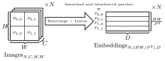
Figure 1: Patch embeddings used in ResMLP and other vision MLPs. The input image ($(N,C,H,W)$ tensor) is divided into patches $P_{i,j}$ which are then linearized and color-channel interleaved. Linearized patches are finally scaled to a configurable hidden dimension $D$ via a linear layer.

II-C Related work

Reviewing other ephemeral approaches to sparsity helped with the development tremendously. One of the most well known examples is dropout [8]. Originally developed as a regularizer, dropout randomly forces activations to zero, sparsifying the connections in a layer. This aims to prevent co-adaption, where feature detectors strongly correlate with other feature detectors, making them useless on their own, which also prevents overfitting. In its original form, dropout induces unstructured sparsity, which is, as established, not suited for compression. There exists a DropBlock [9] variant, which drops spatially contiguous blocks. However, leaving the forward pass unaltered was one of the goals of this work.

Many alternative approaches seek to prune gradients. Sparse gradients are especially beneficial in the context of distributed training, where they have to be broadcasted among compute ranks. Most approaches also prune based on magnitude, using either fixed thresholds or adaptive ones obtained via reduction. Zhang et al. propose a technique called Memorized Sparse Backpropagation [10]. The network essentially estimates a gradient that is empirically shown to be sufficiently similar to the real gradient to effectively train. Unpropagated gradients are still stored for future updates to counteract information loss. While this reduces communication, memory is not saved in this approach. We largely adapt the top-k pruning strategy from this work, however.

A more sophisticated pruning criterion is presented by Liu et al. [11]. Their Dynamic Sparse Training (DST) strategy turns pruning thresholds into learnable parameters. Because the model has to experiment with different configurations, DST uses soft pruning, meaning pruned values are not actually discarded, but masked instead for future use. Combined with the fact that DST focuses on weights this makes this strategy inapplicable to our work.

The closest to our work is Sparse Weight Activation Training (SWAT) [12]. SWAT uses a very similar approach for pruning activations in the context of CNNs, but not with the goal of compression, but faster execution on sparse processor architectures instead. In addition to activation pruning SWAT also adaptively masks weights during the forward computation, similar to dropout. While structured pruning is mentioned, the effects of different granularities of said structure are not explored. As mentioned SWAT focuses on special sparse accelerators in the context of latency based on hardware simulations, while we focus on memory compression and efficient execution on GPUs.

III Block Sparse Operators

In this section we discuss the design and implementation of the block-sparse linear operator developed in the context of this work. While a linear operator is presented here, the technique used can be extended to any operator in principle. Additionally, we report performance for possible configurations using input shapes characteristic to vision MLPs. The benchmarks are performed on an Nvidia A30 GPU.

The block-sparse linear operator is designed to be a plug-in replacement for PyTorch’s nn.linear layer with two additional parameters: the level of sparsity, and the block size of the sparse structure. As mentioned in section I the forward computation is kept dense to ensure an accurate loss computation. After completion of the forward computation, the smallest blocks of input activations are selected using a magnitude based criterion described in further detail in section IV. The selected blocks are forced to zero and the activation tensor is converted to the BSR format. Fig. 2 shows an overview.

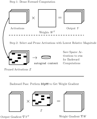
Figure 2: High-level overview of the block-sparse linear operator. After the dense forward computation is completed, blocks of activations are pruned based on magnitude (top-k pruning). The pruned activations are then saved for the backward pass. During the backward pass they are used to calculate the weight gradient via block-sparse matrix multiplication (BSpMM)

A custom CUDA block-sparse matrix multiply (BSpMM) kernel is used to calculate the weight gradient during the backward pass. Because the input and bias gradients do not depend on activations, they can be computed normally using native PyTorch operations. The BSpMM implementation is heavily inspired by CUTLASS. The kernel can be divided into a load and a compute phase. We use vectorized loads and transposition of fragments in shared memory during the load phase to ensure high throughput. To parse the activation’s sparse structure, threads are grouped into cooperative groups with each group being responsible for a BSR block. Each group checks if their respective block is non-zero. If it is zero, the group will skip the load and mark a shared memory internal predicate bit. During the compute phase threads will skip the corresponding dot product calculation, if the predicate vector indicates a zero block. See Fig. 3 for a visualization of the loading process.

(a) Load BSR indices from global memory.

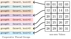
(b) On matching index load non-zero values to registers.

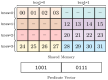
(c) Cache in shared memory

Figure 3: Cooperative thread groups loading a $4\times 8$ BSR encoded tensor with block size $b=4$ to local shared memory. (a): First parse compressed row indices to get the number of non-zero blocks (nnz) in the respective row. Use nnz to access the column index array. (b): If row and column indices found in (a) match the group load corresponding block from global memory to registers. (c): Store loaded values to shared memory for following dot product calculation. We use a bit vector to mark zero blocks in shared memory, so they are skipped during the compute phase Because the number of non-zero blocks is, a priori, unknown enough shared memory has to be allocated to fit a fully dense block in the worst case.

The BSR block size has large implications on the performance of the kernel. Smaller blocks lead to more indices loaded from global memory, lowering the kernel’s FLOP per byte ratio. Also, due to the warp execution style of the GPU, thread divergence may occur at group sizes smaller than the canonical warp size of 32. Another, less obvious, limitation occurs at large BSR block sizes. Because of the limit of 1024 threads per CUDA thread block it becomes necessary to split the logical cooperative groups among multiple thread blocks. Because communication among thread blocks is not allowed, indices for the same logical group will have to be fetched by every participating thread block individually from global memory, negating the benefit of fewer total indices. Generally, increasing sparsity decreases latency. However, performance gains diminish for larger block sizes. At block size 4, the overhead due to decoding makes up a large percentage of the overall execution time. Therefore, lowering this overhead via increased sparsity has a greater effect and vice versa for larger block sizes. Fig. 4 shows the operator’s latency at different block sizes for increasing levels of sparsity.

Measuring throughput at block size 64 for input shapes corresponding to ImageNet, as shown in Figure 5, shows slight speedups over the dense operator for sufficiently large inputs at moderate levels of sparsity (around 50%). For the smaller embedding dimension $D=384$, speedups are achieved even at 10% sparsity. At 90% sparsity we achieve around 140% peak floating point 32 performance. Note that we, of course, calculate throughput in regard to the dense number of floating point operations. While saving memory is the main focus of this work, faster execution is a welcome side effect.

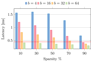
Figure 4: Latency of the BSpMM operator for inputs of shape $(64,196,384)$, different block sizes $b$, and increasing levels of sparsity. The red line marks the latency of PyTorch’s dense torch.matmul routine.

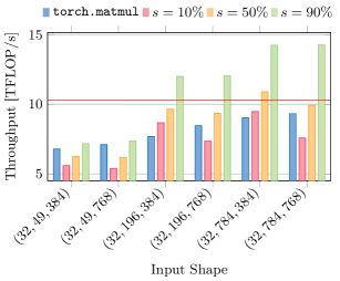
Figure 5: BSpMM throughput at block size 64 compared to dense torch.matmul for common input shapes encountered in ResMLP. Note that FLOPs refers to the dense number of operations in this context. The peak FP32 performance of the A30 GPU used is shown in red.

IV Activation Pruning

In this work we use a simple magnitude-based top-k pruning approach to sparsify activations. To force blocks of activations to zero, their vector or matrix norms are compared and ranked. We then proceed to zero out the $k$ smallest blocks, where $k$ is determined by multiplying the total number of blocks $N$ by the sparsity parameter $s$. The $l2$-norm is chosen to weigh larger individual values stronger and retain a larger total norm of the activation tensor, see Fig. 6.

Blocks are only compared locally, not among other activations in the mini-batch, because there is no direct relationship. For example, one could imagine a darker image being pruned completely otherwise. This makes the comparison computationally inexpensive. Additionally, this also causes all activations in a mini-batch to have the same amount of zero and non-zero blocks, reducing the BSR encoding overhead.

At this time, pruning is performed equally among all layers. For instance, setting sparsity to 50% will force all linear layers in the network to prune 50% of their activations. As other work suggests that different layers have different sensitivity to perturbations [13, 14], future work will analyze each layer’s sensitivity to pruning during training.

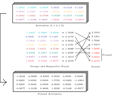
Figure 6: Example top-k block pruning step with block size $3$ at 50% sparsity. We calculate the $l2$-norm per block and select the lowest scoring blocks using top-k. Blocks are only compared within a single activation, not among others in the mini-batch.

V Experiments

We evaluate the feasibility of block-sparse training on the ResMLP-S12 architecture in the context of image classification. Due to time and compute resource constrains, a full parameter grid search over the ImageNet dataset is not viable. We therefore gauge the network’s sensitivity to block-sparsity using the smaller CIFAR10 and CIFAR100 datasets first. Based on the results, we selectively test our method on ImageNet.

V-A Grid Search CIFAR10/100

Fig. 8 shows the top-1 accuracy achieved relative to a densely trained network for various configurations with regard to amount of sparsity and block size. Besides these two parameters, all experiments share the same hyperparameters.

As to be expected, higher levels of sparsity lead to a decrease in accuracy. This effect is stronger at larger block sizes. Intuitively, pruning larger blocks will lead to ”important” values being pruned more often. Interestingly, low levels of sparsity can actually improve accuracy, possibly due to pruning noise acting as a regularizer: as smaller components will no longer contribute, parameter updates become smaller in general.

Similarly, the effects of the block size become more pronounced at higher levels of sparsity. Therefore, smaller block sizes are preferred. For low levels of sparsity, there is no discernible trend. This preference towards smaller block sizes is in direct opposition to our goal of compression. However, viable configurations for $b\geq 16$ can be found up to $70\%$ to $80\%$ of sparsity.

There is some statistical variation in the results. Some configurations perform inexplicably well, like $(s=80\%,b=1)$ for CIFAR10, or badly, like $(s=30\%,b=32)$ for CIFAR100. For reference, running the dense baseline configuration with different weight initialization seeds shows a standard deviation of circa $\pm 1\%$ in top-1 accuracy. Future work should therefore encompass multiple runs per configuration for statistical analysis.

Observing the loss curves for different configurations shows the training to remain stable in terms of spread of the loss curve, see Fig. 7. $b=384$ is chosen as it produces the largest variation in results. Due to the dense forward computation an accurate loss value is obtained. However, because gradient calculation is lossy, parameter updates become less accurate, affecting the rate of convergence. We can observe the loss curves diverging within the first 10 epochs and running almost in parallel afterward.

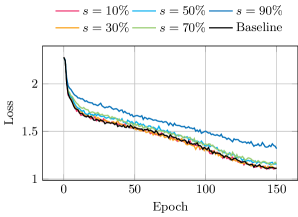
Figure 7: Comparing loss curves at increasing levels of sparsity for ResMLP-S12/CIFAR10. $b=384$ was chosen, as it produces the most extreme split. Because of the dense forward computation, the loss does not become more noisy, only the rate of convergence of the loss curve changes.

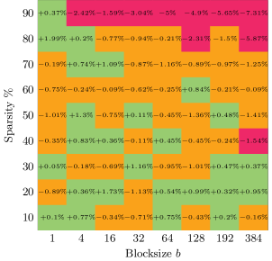
(a)

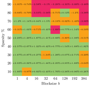
(b)

Figure 8: Heatmap showing the top-1 accuracy relative to dense training for ResMLP-S12 on CIFAR10 (a) and CIFAR100 (b). Values above baseline accuracy are shown in green. Based on the observed standard deviation for dense training we define an arbitrary level of 1.5% below baseline as acceptable. Acceptable values are shown in orange, while accuracies lower than 1.5% below baseline are shown in red.

V-B Early Scaling Experiments

Using the results shown in Fig. 8 as a heuristic, we evaluate block sparse training performance on the ImageNet dataset next. In Fig. 9 we inspect the loss curves, yielding results similar to CIFAR10 and CIFAR100, with a more drastic spread, however. Translating loss to accuracy, $s=60\%$ causes a reduction by $-5\%$ in accuracy, $s=70\%$ causes $-7\%$, and $s=80\%$ leads to $-9\%$ top-1 validation accuracy. However, based on the trends of the loss curves we expect slightly longer training with an adapted learning rate schedule to improve accuracy to near baseline. Further parameter studies are needed of course to conclude this expectation.

To quantify the actual memory saved we additionally log memory allocations via a custom allocator. Table III shows the absolute and relative memory consumed by activations for ImageNet training at mini-batch size 32 for selected potential configurations.

TABLE III: Memory Saved by Pruning (ResMLP-S12/ImageNet, Mini-Batch Size of 32)

Sparsity	Block Size	Activations	$\delta$	$\delta$
$[\%]$	–	[$\mathrm{MiB}$]	[$\mathrm{MiB}$]	$[\%]$
Dense	n.a.	1599.2	–	–
60	16	1234.0	-365.2	-22.8
60	32	1215.0	-384.2	-24.0
60	64	1205.3	-393.9	-24.6
70	16	1161.5	-437.7	-27.4
70	32	1142.9	-456.3	-28.5
70	64	1137.2	-462.0	-29.0
80	16	1082.8	-516.4	-32.3
80	32	1075.1	-524.1	-32.8
80	64	1071.0	-528.2	-33.0

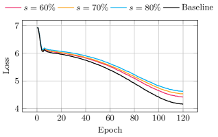
Figure 9: ResMLP-S12/ImageNet loss for $b=16$. A behavior similar to Fig. 7 can be observed. Again, only the rate of convergence is impacted by sparsity. The effect is more severe, however.

VI Discussion

Mini-batch size: A seemingly straight forward alternative to pruning is reducing the mini-batch size. While directly reducing the memory footprint, doing so comes with performance and, moreover, prediction accuracy implications. Fig. 10 shows the latency of training ResMLP-S12/CIFAR10 for one epoch at various mini-batch sizes. For small inputs there is not enough work for the throughput oriented GPU to hide latency. Consequentially, training becomes slower. At larger mini-batch sizes the opposite holds and the training time decreases.

Comparing the training behavior of sparsely and densely trained network at different mini-batch sizes, shows the sparse training to be much closer to dense training at the same mini-batch size. This is shown in Fig. 11, where we compare a densely trained ResMLP-S12 on CIFAR10 to training with 50% sparsity. This comparison is not entirely fair, as 50% sparsity does not translate to 50% less total memory, but based on the observations from Fig. 8 there is potential to move to higher levels of sparsity without sacrificing accuracy. In this regard, Table IV compares the achieved top-1 validation accuracies for different mini-batch sizes. We can see that, on top of training significantly slower, the network loses 7% accuracy going from mini-batch size 32 to 16. Meanwhile, the accuracy for the sparse network at mini-batch size 32 does not differ from the dense network. This could be a valuable alternative in resource-constrained systems, where a viable mini-batch could otherwise not be used due to memory constraints.

TABLE IV: Comparing ResMLP-S12/CIFAR10 Accuracies at Different Mini-Batch Sizes to Sparse Training

Mini-Batch Size	16	32	64	128
Model	Top-1 Accuracy [%]
dense	82	89	91	90
50% sparse	82	89	90	90

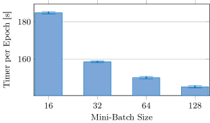
Figure 10: ResMLP-S12/CIFAR10 time per epoch versus mini-batch size. At lower mini-batch sizes the GPU is not utilized optimally, increasing the latency.

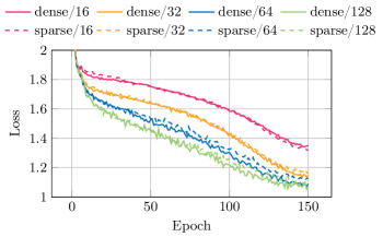
Figure 11: ResMLP-S12/CIFAR10 loss at various mini-batch sizes for dense and sparse training at $s=50\%$. The sparse loss follows the corresponding dense curve very closely performing better than the next smaller mini-batch size.

Overparameterization: Although reasons for this are not yet fully understood, overparameterization of networks, in combination with regularization, seems to lead to better generalization [15, 16, 17]. Our method can be used in this context to increase the model’s complexity to leverage this observation, counteracting the normally associated increase in memory consumption to a degree.

While block sparse training applies to CIFAR10 and CIFAR100 without repercussions in terms of accuracy and without any changes to the training configuration, it seems that, in this configuration, further hyperparameter tuning is required for ImageNet. It is however noteworthy, that at 15 million parameters ResMLP-S12 is a relatively small architecture in the context of the ImageNet dataset. Overparameterization is therefore expected to be low, thus a larger variant is expected to show better results.

Operator implementation: We are also currently working on porting the operator implementation from CUDA to Triton[18] for better portability and extensibility. A block-sparse version of the affine scaling layer found in ResMLP is now also available, potentially allowing for further memory savings, and a convolution operator is planned. A block-sparse convolution operator allows for interesting fundamental comparisons between vision MLPs and CNNs, as the former emulate some of the properties found in the latter. The cross-channel layer mimics the cross-channel property found in plain convolutions. Similarly, the cross-patch layer can be seen as a 1D convolution, mixing information among patches. Effects of differences, like weight sharing, on robustness to block sparsity remain to be observed. CNNs also make for an interesting candidate, as hardware friendly block sizes are relatively small. The most typical kernel sizes in computer vision are $3\times 3$ or $5\times 5$. Due to the multitude of parameters, implementing an efficient block sparse convolutional operator is challenging, however. Nvidia’s cuDNN library, for example, employs different algorithms depending on the parameters via autotuning. Triton might also help in this regard, reducing development time and increasing code readability.

Stochasticity: Related work [19] on gradient compression shows stochastic components to compression to be beneficial. Therefore, future work will also encompass random components in the pruning process. One could imagine randomly swapping blocks near the top-k threshold, resulting in some blocks above the threshold being pruned anyway, and vice-versa below threshold.

VII Summary

We have shown block sparse activation pruning based on a simple top-k criterion to be a viable method for compressing the memory footprint of neural architectures at the example of ResMLP. For CIFAR10/100 we can save around 32% of the memory consumed by activations, which translates to 28% of the total memory footprint, without affecting accuracy significantly. We have additionally demonstrated the scalability of our block-sparse linear operator, maintaining decent latency and throughput for as low as 10% sparsity for adequate block sizes.

Future work will encompass the directions mentioned in the discussion, with an emphasis on larger neural architectures, larger data sets, as well as advanced pruning methods including stochasticity, second-order pruning methods, and more sophisticated pruning schedules.

References

- [1] J. Lee, L. Mukhanov, A. S. Molahosseini, U. Minhas, Y. Hua, J. Martinez del Rincon, K. Dichev, C.-H. Hong, and H. Vandierendonck, “Resource-efficient convolutional networks: A survey on model-, arithmetic-, and implementation-level techniques,” ACM Comput. Surv., vol. 55, no. 13s, Jul 2023. [Online]. Available: https://doi.org/10.1145/3587095
- [2] W. Roth, G. Schindler, M. Zöhrer, L. Pfeifenberger, R. Peharz, S. Tschiatschek, H. Fröning, F. Pernkopf, and Z. Ghahramani, “Resource-efficient neural networks for embedded systems,” CoRR, vol. abs/2001.03048, 2020. [Online]. Available: http://arxiv.org/abs/2001.03048
- [3] Z. Liu, M. Sun, T. Zhou, G. Huang, and T. Darrell, “Rethinking the value of network pruning,” CoRR, vol. abs/1810.05270, 2018. [Online]. Available: http://arxiv.org/abs/1810.05270
- [4] L. Prechelt, “Connection pruning with static and adaptive pruning schedules,” vol. 16, no. 1, pp. 49–61. [Online]. Available: https://www.sciencedirect.com/science/article/pii/S0925231296000549
- [5] G. Schindler, W. Roth, F. Pernkopf, and H. Froening, “Parameterized Structured Pruning for Deep Neural Networks,” CoRR, vol. abs/1906.05180. [Online]. Available: http://arxiv.org/abs/1906.05180
- [6] H. Touvron, P. Bojanowski, M. Caron, M. Cord, A. El-Nouby, E. Grave, G. Izacard, A. Joulin, G. Synnaeve, J. Verbeek, and H. Jégou, “ResMLP: Feedforward networks for image classification with data-efficient training,” CoRR, vol. abs/2105.03404. [Online]. Available: http://arxiv.org/abs/2105.03404
- [7] A. Dosovitskiy, L. Beyer, A. Kolesnikov, D. Weissenborn, X. Zhai, T. Unterthiner, M. Dehghani, M. Minderer, G. Heigold, S. Gelly, J. Uszkoreit, and N. Houlsby, “An Image is Worth 16x16 Words: Transformers for Image Recognition at Scale,” CoRR, vol. abs/2010.11929. [Online]. Available: http://arxiv.org/abs/2010.11929
- [8] G. E. Hinton, N. Srivastava, A. Krizhevsky, I. Sutskever, and R. R. Salakhutdinov, “Improving neural networks by preventing co-adaptation of feature detectors,” CoRR, vol. abs/1207.0580. [Online]. Available: http://arxiv.org/abs/1207.0580
- [9] G. Ghiasi, T.-Y. Lin, and Q. V. Le, “DropBlock: A regularization method for convolutional networks,” CoRR, vol. abs/1810.12890. [Online]. Available: http://arxiv.org/abs/1810.12890
- [10] Z. Zhang, P. Yang, X. Ren, Q. Su, and X. Sun, “Memorized sparse backpropagation,” vol. 415, pp. 397–407. [Online]. Available: https://www.sciencedirect.com/science/article/pii/S0925231220313357
- [11] J. Liu, Z. Xu, R. Shi, R. C. C. Cheung, and H. K. H. So, “Dynamic Sparse Training: Find Efficient Sparse Network From Scratch With Trainable Masked Layers,” CoRR, vol. abs/2005.06870. [Online]. Available: http://arxiv.org/abs/2005.06870
- [12] M. A. Raihan and T. Aamodt, “Sparse Weight Activation Training,” in Advances in Neural Information Processing Systems, vol. 33. Curran Associates, Inc., pp. 15 625–15 638. [Online]. Available: https://proceedings.neurips.cc/paper/2020/hash/b44182379bf9fae976e6ae5996e13cd8-Abstract.html
- [13] H. Borras, B. Klein, and H. Fröning, “Walking noise: Understanding implications of noisy computations on classification tasks,” CoRR, vol. abs/2212.10430, Dec 2022. [Online]. Available: https://arxiv.org/abs/2212.10430
- [14] T. Krieger, B. Klein, and H. Fröning, “Towards hardware-specific automatic compression of neural networks,” CoRR, vol. abs/2212.07818, Dec 2022. [Online]. Available: https://arxiv.org/abs/2212.07818
- [15] C. Zhang, S. Bengio, M. Hardt, B. Recht, and O. Vinyals, “Understanding deep learning (still) requires rethinking generalization,” Communications of the ACM, vol. 64, no. 3, pp. 107–115, Feb. 2021. [Online]. Available: https://dl.acm.org/doi/10.1145/3446776
- [16] J. Kaplan, S. McCandlish, T. Henighan, T. B. Brown, B. Chess, R. Child, S. Gray, A. Radford, J. Wu, and D. Amodei, “Scaling Laws for Neural Language Models,” CoRR, vol. abs/2001.08361. [Online]. Available: http://arxiv.org/abs/2001.08361
- [17] Z. Li, E. Wallace, S. Shen, K. Lin, K. Keutzer, D. Klein, and J. Gonzalez, “Train Big, Then Compress: Rethinking Model Size for Efficient Training and Inference of Transformers,” in Proceedings of the 37th International Conference on Machine Learning. PMLR, pp. 5958–5968. [Online]. Available: https://proceedings.mlr.press/v119/li20m.html
- [18] P. Tillet, H. T. Kung, and D. Cox, “Triton: An intermediate language and compiler for tiled neural network computations,” in Proceedings of the 3rd ACM SIGPLAN International Workshop on Machine Learning and Programming Languages - MAPL 2019. ACM Press, pp. 10–19. [Online]. Available: http://dl.acm.org/citation.cfm?doid=3315508.3329973
- [19] D. Alistarh, D. Grubic, J. Li, R. Tomioka, and M. Vojnovic, “Qsgd: Communication-efficient sgd via gradient quantization and encoding,” CoRR, vol. abs/1610.02132, 2017. [Online]. Available: http://arxiv.org/abs/1610.02132