Attentional Graph Neural Networks Is All You Need for Robust Massive Network Localization
Abstract
In recent years, Graph neural networks (GNNs) have emerged as a prominent tool for classification tasks in machine learning. However, their application in regression tasks remains underexplored. To tap the potential of GNNs in regression, this paper integrates GNNs with attention mechanism, a technique that revolutionized sequential learning tasks with its adaptability and robustness, to tackle a challenging nonlinear regression problem: network localization. We first introduce a novel network localization method based on graph convolutional network (GCN), which exhibits exceptional precision even under severe non-line-of-sight (NLOS) conditions, thereby diminishing the need for laborious offline calibration or NLOS identification. We further propose an attentional graph neural network (AGNN) model, aimed at improving the limited flexibility and mitigating the high sensitivity to the hyperparameter of the GCN-based method. The AGNN comprises two crucial modules, each designed with distinct attention architectures to address specific issues associated with the GCN-based method, rendering it more practical in real-world scenarios. Experimental results substantiate the efficacy of our proposed GCN-based method and AGNN model, as well as the enhancements of AGNN model. Additionally, we delve into the performance improvements of AGNN model by analyzing it from the perspectives of dynamic attention and computational complexity.
Index Terms:
Graph neural networks, attention mechanism, massive network localization, non-line-of-sight.I Introduction
Graph Neural Networks (GNNs) have recently achieved several state-of-the-art results across a variety of graph-related learning tasks, such as node classification, link prediction, and graph classification [2, 3, 4, 5]. Unlike Multi-Layer Perceptrons (MLPs), GNNs leverage the topological structure of graphs, where each node aggregates data from its neighbors through connected edges, thus enriching its representation beyond its own attributes [6, 7]. This ability to harness relational information endows GNNs a distinct superiority in handling complex, interconnected data. Despite their effectiveness, GNN models are primarily employed in handling classification tasks that involve discrete labels. Conversely, the complex challenge of regression problems, which represent a substantial portion of practical applications in signal processing, remains underexplored in academic research despite its significance.
Recently, attention mechanisms have garnered widespread interest in numerous sequential learning tasks [8, 9]. The underlying principle involves learning a function that aggregates input data, with a particular emphasis on elements pertinent to a given context. This concept is referred to as self-attention when a single sequence serves as both the input and context. With the success of the attention mechanism [10], the integration of this mechanism with GNNs provides a promising approach to attaining state-of-the-art performance in regression tasks.
In this paper, we delve into a classic yet challenging nonlinear regression problem of large-scale network localization, a critical task that requires precise measurements both between agent nodes and anchor nodes, and among the agent nodes themselves. Over recent decades, a variety of canonical methods have been developed to tackle this issue, ranging from maximum likelihood [11, 12, 13, 14] and least-squares [15] estimation methods to multi-dimensional scaling [16], mathematical programming [17, 18], and Bayesian message passing approaches [19, 20]. Despite their diversity, a major challenge these methods face is the impact of non-line-of-sight (NLOS) propagation, which can incur severe performance degradation of the localization process by introducing biased distance estimation.
To combat the issue of NLOS, the most applied strategy is to perform NLOS identification for each link, and either discard or suppress the NLOS measurements [21]. However, accurate NLOS identification requires large-scale offline calibration and huge manpower. The NLOS effect can also be dealt with from an algorithmic aspect. Based on the assumption that NLOS noise follows a certain probability distribution, the maximum likelihood estimation based methods handling NLOS were developed in [22, 23]. Yet, this approach is prone to performance deterioration due to model mismatches. More recently [24, 25], the network localization problem is formulated as a regularized optimization problem in which the NLOS-inducing sparsity of the ranging-bias parameters was exploited. Unfortunately, all of these methods are computationally expensive for massive networks, which makes the aforementioned methods less feasible for large-scale applications.
Considering all these factors, we propose integrating attention mechanisms and GNN models for network localization tasks. Experimental evaluations demonstrate the approach’s exceptional stability and high accuracy in localization, even under severe NLOS conditions, along with significantly reduced computational time in massive network sizes. Notably, these methods eliminate the need for laborious offline calibration and NLOS identification processes, making them well-suited for real-world deployment. To the best of our knowledge, this represents the inaugural application of GNNs in the field of network localization. The main contributions are summarized as follows.
-
•
We introduce an innovative graph convolutional network (GCN)-based network localization method, which we originally proposed in [1]. This approach provides an excellent solution to large-scale network localization in terms of accuracy, robustness, and computational time. Importantly, this represents the first application of GNNs in network localization.
-
•
To address the optimal hyperparameter selection issue and enhance the limited model expressiveness of the GCN-based model, we propose an attentional graph neural network (AGNN) model, consisting of two crucial modules. These modules are specifically designed with distinct attention architectures to address two issues associated with GCN, and extensive experiments demonstrate the effectiveness of the AGNN model.
-
•
We provide an in-depth analysis of the performance improvements of the AGNN model, demonstrating the dynamic attention property of the two specifically designed attention architectures in AGNN. Additionally, we present a complexity analysis for all models.
The remainder of this paper is organized as follows. The background of network localization and problem formulation are introduced in Sec. II. In Sec. III, we introduce the GCN framework for network localization. To extend to more general scenarios, AGNN model is proposed in Sec. IV. Finally, we conclude the paper in Section VII.
Notation: Boldface lowercase letter and boldface uppercase letter are conventionally used to signify vectors and matrices, respectively. and designate the -th column and row of matrix , respectively. Meanwhile, the element in the -th row and -th column of matrix is denoted by . The calligraphic letter is employed to denote a set, where signifies the cardinality of this set. represents the set of natural numbers from to . The operator signifies vector/matrix transpose. represents the Euclidean norm of a vector. denotes the Frobenius norm of a matrix. stands for the column/row concatenation operation for two column/row vectors. represents the Hadamard product of two matrices with identical dimensions.
II Background and Problem Formulation
II-A Localization Scenario
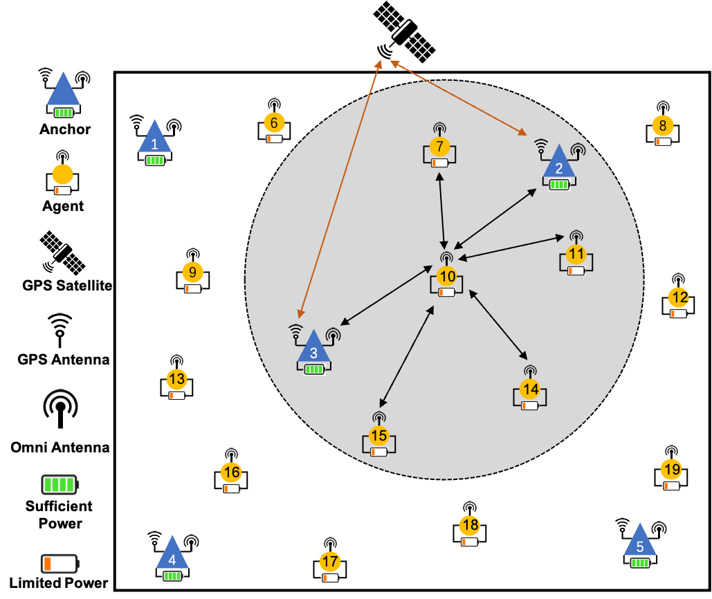
Fig. 1 illustrates a classic wireless network localization scenario. In the context of a massive wireless network, only a limited number of nodes, known as anchors, possess precise location information obtained through GPS/BeiDou chips. Conversely, the remaining nodes, referred to as agents, lack access to GPS and consequently need to be located. Equipped with omni-directional antennas, each node broadcasts signals containing information such as node ID, transmit power, transmit time, and network configurations.
This scenario is highly representative of many real-world massive wireless networks. For instance, in a 5G network, a substantial number of small base stations are densely deployed within each cell. Similarly, in Internet of Things (IoT) network, which advocates the interconnection of a wide array of devices and machines [26], there is a substantial number of interconnected smart devices. Moreover, in the metaverse, a burgeoning virtual reality ecosystem, numerous virtual spaces host a myriad of interconnected users, avatars, and digital entities [27]. In such massive networks, it is common that only a small fraction of nodes possess their precise locations. Traditionally, to determine the locations of all nodes, either significant human resources must be allocated for offline calibration, or, as an alternative, costly and power-intensive GPS/Beidou chips must be installed in every node. To algorithmically address this issue, we formalize the localization problem as follows.
II-B Problem Formulation
We consider a wireless network in a two-dimensional (2-D) space, with the extension to 3-D case being straightforward. We let be the set of indices for the anchors, whose positions are known and fixed, and be the set of indices for the agents, whose positions are unknown.
In accordance with numerous established studies, e.g., [23], the measured distance between any two nodes and can be represented as follows:
| (1) |
where is defined as the Euclidean distance between nodes . accounts for an additive measurement error arising from line-of-sight (LOS) and non-line-of-sight (NLOS) propagation, and it can be further detailed as follows:
| (2) |
Here, the LOS noise, , follows a zero-mean Gaussian distribution, i.e., , , while the NLOS bias, , is generated from a positive biased distribution. is sampled from the Bernoulli distribution with being the NLOS occurrence probability [28]. Consequently, a measurement matrix, denoted by , can be constructed by stacking the measured distances, i.e., the -th entry of is . Notably, we consider a symmetric scenario where and for .
The measured distances can be estimated from the received signal strength (RSS), or the time of arrival (ToA) measurements, which can be acquired through diverse technologies, including cellular networks, WLAN, ultra-wideband radio frequencies, as well as ultra and audible sound. However, NLOS propagation can introduce significant time delays in ToA measurements and substantial signal attenuation in RSS measurements [29], thereby impeding the accuracy of distance estimation.
Building on the aforementioned formulations, our primary objective is to precisely localize the agents within a massive wireless network while ensuring satisfactory computation time. To achieve this, we propose a novel GNN-based localization paradigm, specifically the GCN-based network localization. This approach is data-driven and leverages a graph-based machine learning model, the details of which will be elaborated upon in the subsequent section.
III Network Localization with Classic GCN
In this section, we first introduce a GCN-based data-driven method for network localization, that was originally proposed in [1]. Subsequently, we provide some key findings regarding the reasons behind the exceptional performance of this model. Lastly, we discuss some limitations of our method that necessitate further improvement.
III-A Graph Convolutional Network
Among various different GNN models, graph convolutional networks (GCNs) represent a prominent category. In this subsection, our focus lies on the formulation of the network localization problem utilizing the classic GCNs.
We formally define an undirected graph associated with a wireless network as , where denotes the set of nodes in the network, including anchors and agents, and is a symmetric adjacency matrix. In traditional GCNs, each element of represents the weight of the edge connecting nodes and , which can be inherently interpreted as a measure of similarity between nodes and . While, in the context of network localization, the concept of similarity is particularly relevant to proximity, essentially indicated by the Euclidean distance between nodes. To integrate this concept into our method, we introduce an Euclidean distance threshold, denoted as , to determine the existence of an edge between any two nodes, i.e., whether two nodes are proximal. Therefore, by applying this threshold, the adjacency matrix is constructed as follows:
| (3) |
As further elaborated in Sec. III-B, this threshold plays a crucial role in localization performance. And we also need to note that includes self-connections, making it an augmented adjacency matrix. Additionally, we denote the associated degree matrix of as , which is a diagonal matrix with . Based on these definitions, we can construct a truncated measurement matrix which only contains those measured distances that are smaller than or equal to .111In , many entries are zeros, representing distances between nodes that exceed . From a physical distance perspective, setting the excluded distances to zero might be challenging to comprehend. However, from a mathematical computation standpoint, since will be multiplied with a trainable matrix in a subsequent step, omitting values by setting them to zero or leaving them as null does not affect the matrix operations. Therefore, it can be understood that setting the excluded values to zero is mathematically equivalent to treating them as null values.
With the well-defined graph, we propose our GCN-based method as follows. We first denote the node representation at the -th layer as , where is the hidden dimension of -th layer. And the initial node representation is set to be the truncated measurement matrix, i.e., . In each layer, a feature propagation step will be implemented first by the following updated process:
| (4) |
where signifies the normalized adjacency matrix [2], and represents the hidden representation matrix in the -th graph convolution layer. Conceptually, this step effectively smoothens the hidden representations within the local graph neighborhood, thereby promoting similar predictions for closely connected nodes. Following the feature propagation step, the subsequent two stages of GCN, namely linear transformation and nonlinear activation, are implemented as usual. Precisely, the -th layer contains a layer-specific trainable weight matrix and an element-wise nonlinear activation function , such as [30]. The updating rule for the node representation at the -th layer is given by:
| (5) |
Taking a 2-layer GCN as an example, the estimated positions, denoted as , are determined by the following equation:
| (6) |
The weight matrices and can be optimized by minimizing the mean squared error (MSE), defined as , between the true positions of anchors and the respective estimations . Then, the optimization problem for GCN-based network localization method can be expressed as follows:
III-B Key Findings of GCN
The numerical results, as detailed in Section VI, illustrate the substantial improvements realized by adopting the GCN-based approach over various benchmark methods. In the subsequent discussion, we probe into some key findings that shed light on the factors contributing to the remarkable success of this model. These insights are instrumental in understanding the efficacy of the GCN-based approach, confirming its aptness for network localization, and providing guidance for further refinement of the model.
We pinpoint two major factors: the threshold and the normalized adjacency matrix . In the following, we will analyze these factors individually.
III-B1 Effects of Thresholding
Thresholding serves two primary functions: 1) the truncation of significant noise, and 2) the prevention of over-smoothing.
Noise truncation. Recalling the definition of , for each non-zero , the condition holds. Consequently, the operation , as described in Sec. III-A, implies that comprises only those measurements that are below the threshold and accompanied by confined noise. For those measurements with the existence of NLOS noise, this condition can be further expressed as with . By applying an appropriate threshold, we not only constrain the distance but also truncate the noise, such that measurements are retained only if two nodes are adjacent and primarily affected by a small or moderate measurement noise.
Avoiding over-smoothing. Consider an extreme case where the threshold is too large to lose effect, resulting in the corresponding graph becoming fully connected and the adjacency matrix being an all-ones matrix. In this scenario, as described by Eq. (4), all rows of the hidden representation matrix become identical. This signifies that the obtained hidden representation entirely loses its ability to distinguish nodes. As a result, the predicted positions of all nodes tend to converge towards a single point. This phenomenon is commonly referred to as over-smoothing. Therefore, it is imperative to select an appropriate threshold to prevent such detrimental effects.
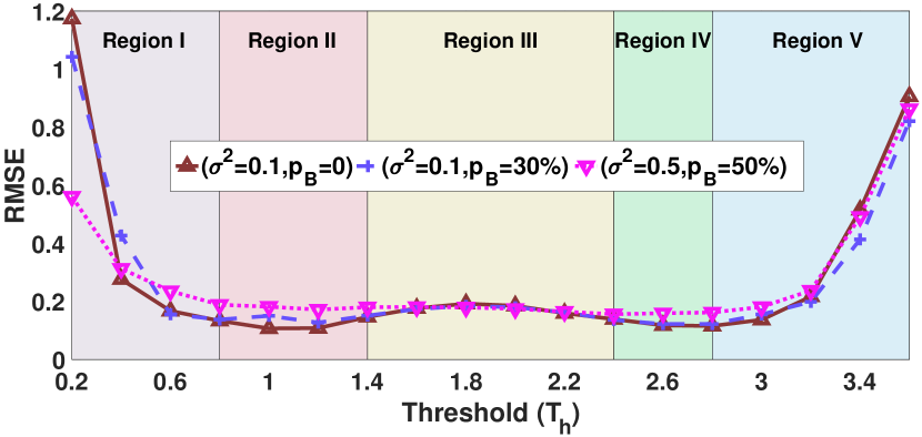
To provide a more comprehensive elucidation of the influence of the threshold, , on the localization performance, we conducted an experiment that systematically explores the RMSE of GCN across a range of within three distinct noise scenarios, as depicted in Fig. 2. Based on these results, we can classify the localization performance into five distinct regions, each aligned with a specific range of threshold values.
In Region I, initial performance issues stem from insufficient graph edges when is set too low, leading to isolated nodes that hinder effective localization, thereby reducing overall accuracy. Within Regions II to IV, a counterbalance is observed between the NLOS noise truncation effect (Region II) and the growing number of neighbors per node (Region IV). Region V exhibits a sharp increase in RMSE attributable to a weakened noise truncation effect and a pronounced over-smoothing problem. For detailed experimental settings and result descriptions, please refer to our previously published paper [1].
III-B2 Effects of
To comprehend the superior localization performance of GCN, we also analyze the effects of the normalized adjacency matrix, , from both spatial and spectral perspectives.
Spatial perspective–Aggregation and combination. To understand the spatial effect of , we disassemble , cf. Eq. (4), into two components:
| (8) |
In essence, Eq.(8) encapsulates two critical operations: aggregation and combination. Aggregation (Eq.(8)-[ii]) captures the features of neighboring nodes in accordance with the predefined graph structure. Subsequently, additive combination of the aggregated neighboring information and the intrinsic information (Eq.(8)-[i]) of each individual node takes place. As a result, in GCN, the hidden representation of each labeled node (i.e., anchor in the localization setting) is a weighted summation of those of its neighbors. Essentially, GCN leverage the attributes of both labeled and unlabeled nodes in its training process, thereby contributing to its superior performance in network localization.
Spectral perspective–Low-pass filtering. From the spectral perspective, The feature propagation step in Eq.(8) can be rewritten as
| (9) | ||||
| (10) | ||||
| (11) |
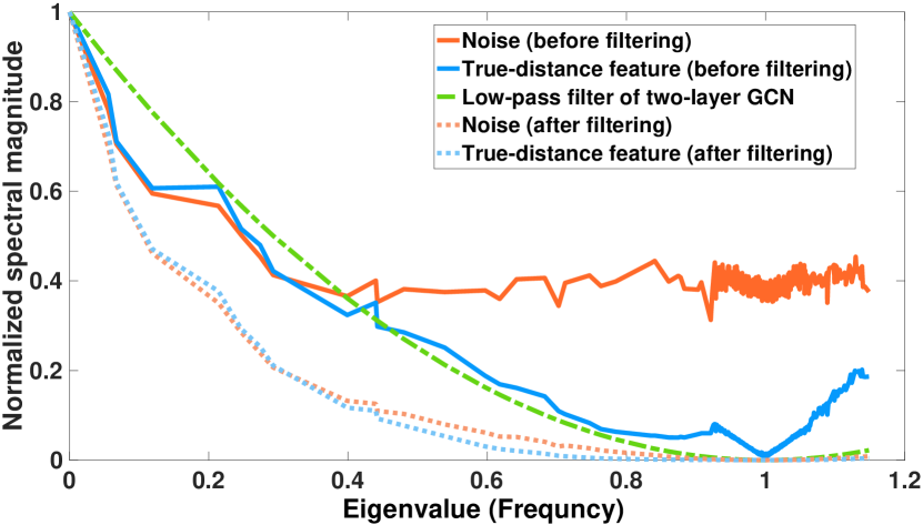
where denotes the normalized Laplacian, and are the associated eigenvectors and eigenvalues. In terms of graph signal operations, and correspond to the Graph Fourier Transform and Inverse Graph Fourier Transform, respectively. The vector and scalar represent the -th graph Fourier basis and “frequency” component of the graph signal, respectively [33, 34]. According to Eq.(11), each feature propagation operation acts as a spectral “low-pass” filter , and the two-layer GCN can be viewed as applying a filter [35]. This spectral filtering concept is essential for understanding how GCNs process and filter signal information across the network. Fig. 3 illustrates the “frequency” components of the LOS noise and the true distance matrix before and after filtering. Notably, in the unfiltered state, the majority of information within the true distance matrix is concentrated in the “low-frequency” band. Conversely, the LOS noise displays both “low-frequency” and “high-frequency” components before filtering. Comparing the results before and after filtering, it becomes evident that the normalized adjacency matrix , serving as a ’low-pass’ filter, effectively mitigates the “high-frequency” component of the LOS noise. From a spectral analysis standpoint, this ’low-pass’ filtering capability of justifies the improved performance of GCNs in localization tasks by filtering out the “high-frequency” component of noise.
III-C Limitations of Classic GCN
From the preceding discussion, it is evident that the proposed GCN-based model is highly suitable for network localization tasks. Nevertheless, the subsequent discussion has uncovered several limitations inherent to this model. Recognizing and subsequently addressing these limitations is crucial for further enhancing the model’s robustness and applicability in real-world scenarios. The primary limitations can be summarized as follows:
Optimal threshold issue. As shown in Fig. 2, the selection of threshold plays a pivotal role in determining the localization performance. However, as a hyperparameter, determining the optimal value for this threshold is not straightforward, particularly in diverse noise and network size scenarios. Furthermore, due to the distinct node positions and varying channel state information, each node may possess its unique optimal threshold, rather than a uniform threshold applicable to all nodes. Consequently, there arises a necessity to develop a more flexible model, one that is capable of autonomously learning the optimal threshold during the training process.
Limited model expressiveness. Under Eq. (8), the GCN-based model employs a constant aggregation weight, determined by adjacency and node degree, which constrains its capacity to adaptively aggregate and combine information from neighboring nodes . From the spectral perspective, the GCN-based model exclusively represents a fixed graph convolutional filter, as delineated by a green dash-dot line in Fig. 3. This fixed filtering characteristic (fixed adjacency matrix) compromises its versatility, especially when confronted with complex network scenarios that demand customized filters at each graph convolutional layer.
In the following, we turn our focus to offering effective solutions to mitigate the aforementioned issues by introducing an Attentional GNN (AGNN) model.
IV Network Localization with AGNN
In this section, we concentrate on the design of a fresh AGNN model that possesses the capability to autonomously determine the optimal threshold and adaptively determine the aggregation weight of each node for various network localization task.
IV-A Attention Mechanism for Network Localization
Motivated by recent advancements in attention-based graph neural networks, such as GAT [4] and GATv2 [36], we incorporate the attention mechanism into the network localization task. This adaptation is expected to enable the model to autonomously determine neighbor sets for each node and acquire flexible aggregation weights for all pairs of nodes based on attention scores.
Graph attention architectures typically consist of a sequence of graph attention layers [4]. To elucidate, we start by explaining the basic structure of a single graph attention layer. Each layer incorporates at least one learnable linear transformation for learning higher-level representations, which is parameterized by a weight matrix and is applied to every node . Subsequently, a shared attentional mechanism, denoted as , is conducted to calculate the attention scores between node and as
| (12) |
These scores effectively quantify the relative importance of node ’s features with respect to those of node . In general, Eq. (12) enables each node to compute an attention score concerning every other node.
In GAT/GATv2, given a known graph structure, attention scores serve as weights for edges in the adjacency matrix and participate in the feature propagation in Eq. (8). In network localization tasks without a predefined threshold , where the graph structure is unknown, an initial assumption is made of a complete graph. An attention mechanism is then employed to compute scores for all node pairs, aiming to prioritize nearby nodes for optimal neighbor selection. Nonetheless, directly computing attention scores for all possible node pairs poses two significant challenges:
1) High computational complexity. As the number of nodes increases, the number of possible node pairs grows quadratically. Therefore, computing attention scores for all possible node pairs is computationally intensive and time-consuming. This issue can significantly slow down the training of the attention mechanism, especially when dealing with large-scale graphs.
2) Over-smoothing issues. Similar to the analysis in Sec. III-B, in a complete graph, each node’s representation necessitates aggregation with those of all other nodes. This aggregation results in a convergence of distance-related information across all nodes, ultimately giving rise to the over-smoothing issue. Remarkably, despite assigning diverse attention scores to edges, the graph attention mechanism fails to effectively mitigate over-smoothing, and its expressive power diminishes exponentially with increasing model depth [37].
To tackle this challenge, we introduce a novel AGNN model for network localization tasks in the subsequent sections. This model is explicitly crafted to autonomously acquire graph structures during the training process, making it highly suitable for network localization tasks across diverse network scenarios.
IV-B Overview of AGNN Model
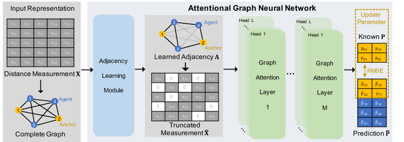
We propose the AGNN model tailored for network localization tasks, which is composed of an Adjacency Learning Module (ALM) and Multiple Graph Attention Layers (MGALs), as illustrated in Fig. 4. The ALM leverages an attention mechanism to learn a distance-aware threshold. In other words, nodes can adaptively adjust the threshold based on the true distance to their neighbors, enabling more flexible neighbor selection. Subsequently, the MGALs utilize another attention-based mechanism to acquire adaptable aggregation weights based on the adjacency matrix learned by ALM.
The ALM autonomously determines the neighbor set for each node based on the attention mechanism. This approach is capable of learning an adjacency matrix, thereby significantly reducing computational complexity and effectively addressing the over-smoothing issue associated with the direct utilization of the graph attention mechanism. Next, we delve into the details of the ALM.
IV-C Adjacency Learning Module
To adaptively learn the optimal threshold during the training process, we propose the ALM, which incorporates an attention mechanism to learn the specific threshold for each node pair. Nevertheless, directly learning the individual threshold for each pair without any prior knowledge of the graph structure can be computationally expensive. To mitigate this, ALM employs a two-step process: initially, a coarse-grained neighbor selection is conducted using a manually-set threshold, followed by a fine-grained neighbor refinement through an attention mechanism. In the following, we will provide the details of these two stages of ALM.
Stage I: coarse-grained neighbor selection. To address the challenge of computing attention scores without prior knowledge of the graph structure, we initially utilize a preselected threshold, , to perform a coarse-grained neighbor selection for each node, following the procedure in Eq. (3). Notably, unlike the threshold in the GCN-based model which can significantly influence the localization accuracy, this initial threshold can be chosen from a broader range, as our objective here is to establish a coarse-grained neighbor set, , for each node , thereby reducing the computational complexity and alleviating the over-smoothing issue.
Stage II: fine-grained neighbor refinement. To facilitate fine-grained neighbor set learning within each previously identified coarse-grained neighbor set, we introduce a distance-aware threshold matrix based on attention scores. This matrix is employed to further refine the previously coarse-grained neighbor sets by comparing them with the measured distance values.
Specifically, we incorporate the masked attention mechanism [10] into the coarse-grained graph structure. This means we compute the attention scores only for nodes within the coarse-grained neighbor set of node . Our designed attention scores is calculated as follows:
| (13) |
Here, represents the element-wise absolute value of a vector . The attention mechanism in this context consists of a two-layer neural network, parametrized by an attention weight vector and an attention weight matrix , and applies a nonlinear mapping , such as LeakyReLU.
The reasons for using Eq. 13 to compute the attention scores, as opposed to a single-layer neural network used in GAT [4] and GATv2 [36], are as follows:
-
•
Passing each node’s feature through a linear transformation with followed by a nonlinear activation function enhances the expressive power of feature transformations;
-
•
Taking the absolute difference between two transformed representations can be regarded as a learnable distance metric between their representations, which possess the symmetry property that is not considered by GAT and GATv2 but is essential for network localization;
-
•
The attention vector learns an effective dimensionality reduction mapping to project the learnable distance metric into a scalar, serving as the output attention score.
To convert the attention scores into thresholds and ensure the thresholds are comparable to the measured distances, we apply nonlinear scaling through:
| (14) |
where identifies the maximum value from the row vector . Using Eq. (14), we obtain a distance-aware threshold matrix denoted as . With the distance-aware thresholds obtained within each coarse-grained neighbor set, we establish a criterion for selecting fine-grained neighbors by comparing the measured distance with the thresholds. Specifically, the adjacency and the truncated measured distance can be represented as follows:
| (15) |
and further construct the truncated measurement matrix as .
Nevertheless, Eq. (15), formulated as a step function, lacks differentiability concerning , which is the parameter we intend to train using gradient-based optimization methods. Typically, conventional approaches often employ a Sigmoid function as an approximation for the step function. Yet, this strategy is unsuitable for our objective of achieving a sparse adjacency by eliminating elements surpassing the threshold. For instance, the result of is close but not equal to . Consequently, it is essential to identify an approximation for Eq. (15) that is both differentiable concerning the trainable threshold vector and capable of filtering out values exceeding the threshold.
Based on the above requirements, we develop an appropriate approximating step function that addresses this issue. The approximating step function can be defined as follows:
| (16) |
where is a hyperparameter adjusting the steepness of the hyperbolic tangent (tanh) function.
Subsequently, the approximation of Eq. (15) and relative expression of can be expressed as:
| (17) | ||||
| (18) |
It is evident that our devised approximating step function, employing ReLU and tanh, yields a notably sharper transition on one side and effectively truncates values to zero on the other side, consequently achieving a more accurate approximation of the step function than the Sigmoid function. Moreover, its derivative can be obtained everywhere 222In the standard definition of ReLU, the derivative at 0 is typically taken to be 0., which makes it feasible to compute gradients respective to the trainable threshold.
After obtaining the adjacency matrix and truncated measurement matrix via the attentional method, they can be effectively used as inputs for the graph attention layer.
IV-D Multiple Graph Attention Layers
We assume that the final neighbor set of each node has been generated through ALM, denoted as for node . Subsequently, we introduce MGALs, a more generalized form of the graph attention mechanism inspired by GATv2 [36], to learn the aggregation weight and predict the positions of all nodes.
We commence by elucidating the -th single graph attention layer, serving as the foundational layer applied uniformly across the entirety of MGALs. Here, we employ a single layer feed-forward neural network, parametrized by an attention weight vector and an attention weight matrix , as the attention mechanism . Then, for , the computation of attention scores in Eq. (12) can be expressed as:
| (19) |
| (20) |
Here, denotes the weight matrix in the -th graph attention layer.
Notably, we use two distinct learnable weight matrices, and , with distinct functionalities in our approach. in Eq. (19) functions as a linear transformation, converting input representations into higher-level representations. Conversely, collaborates with the weight vector to establish an attentive rule, determining the correlation between each pair of nodes. Moreover, the proposed graph attention layer represents a more generalized form than GATv2 and can be reduced to GATv2 when assumes an identity matrix.
To make the attention scores comparable across different nodes, we normalize them across all choices of using the function:
| (21) |
Once obtained, the normalized attention scores are used to update with nonlinearity as:
| (22) |
Furthermore, in line with [10], employing multi-head attention can contribute to stabilizing the learning process. Specifically, there are attention mechanisms, or heads, independently executing the transformation of Eq. (22). The features generated by each head are then concatenated, yielding the following updated hidden features:
| (23) |
Note that, in this multi-head setting, the updated hidden feature, , will have a dimensionality of (rather than ). Particularly, on the final (prediction) layer of the network, we employ averaging instead of concatenation to obtain the final output.
IV-E Optimization Problems for AGNNs
In summary, we have proposed an ALM capable of autonomously learning optimal thresholds for individual edges through an attention mechanism. This ALM further acquires an adaptive adjacency matrix and the corresponding truncated measurement matrix. Subsequently, MGALs leverage these learned matrices and employ another attention mechanism to acquire adaptable aggregation weights, enhancing the expressiveness of the model. As a result, it effectively addresses the limitations of the classic GCN, as discussed in Section III-C. Hereafter, we formulate the optimization problem for our proposed AGNN as follows:
| (24) | ||||
Here, and denote all trainable matrices in ALM and MGALs, respectively.
V PERFORMANCE ANALYSIS
In this section, we analyze our proposed AGNN model from the perspectives of two fundamental properties: dynamic attention property and complexity analysis. Through theoretical analysis333For the sake of clarity, we assume a complete graph in the subsequent discussions. Analogous results can be extrapolated to the case of incomplete graph. The key distinction is that the neighbor set of each node in the incomplete graph scenario becomes a subset of the corresponding set in a complete graph., we aim to elucidate the reasons behind the superior performance of AGNN in terms of model representational capacity, and computational complexity.
V-A Dynamic Attention Property
In general, attention serves as a mechanism to compute a distribution over a set of input key vectors when provided with an additional query vector. In the context of network localization, the query vector and input key vectors represent the feature vectors of a target node and its neighbors, respectively. The attention mechanism in network localization involves the process of learning how to allocate attention weights to all neighboring nodes concerning the target node. In this subsection, we have demonstrated that, in contrast to the classical GAT model [4] which is confined to computing static attention and thereby encounters significant limitations, our proposed graph attention mechanism is designed to inherit the capabilities of dynamic attention [36].
When an attention function consistently assigns the highest weight to the same neighbor node regardless of the target node, we refer to this type of attention as static attention. Static attention exhibits limited flexibility in the scenario of network localization, as the neighbor with the highest attention weight is invariably selected given a proper threshold, regardless of the target node and attention function.
A more general and potent form of attention is dynamic attention [36]. Compared to static attention, dynamic attention offers greater flexibility and adaptability. A dynamic attention function can assign the highest weight to discretional neighbor, rather than rigidly assign to a specific neighbor node. This allocation depends on the feature vectors of the target and neighboring nodes, as well as the chosen attention function.
In the classical GAT model [4], a scoring function is employed to compute a score for every edge , which indicates the importance of the features of the neighbor to the node :
| (25) |
Nonetheless, as proven in [36]:
Theorem 1
A GAT layer computes only static attention, for any set of node representations . In particular, for , a GAT layer does not compute dynamic attention.
Proof : Refer to [36].
The primary issue with the scoring function (25) in the standard GAT is that the learned weights, and , are applied in succession, which allows them to be condensed into a single linear layer.
Compared with the standard GAT, each graph attention layer (19) in MGALs simply applies the attention weight matrix after the concatenation, and the attention weight vector after the nonlinearity . Next, we show that our proposed graph attention layer addresses the limitation of static attention in GAT and possesses a significantly more expressive dynamic attention property.
Theorem 2
Proof : See App. VIII-A.
The core idea presented in this proof around the principle that the graph attention function in Eq. (19, 20) can be interpreted as a single-layer graph neural network. Consequently, it can be a universal approximator [38] of an appropriate function we define, thereby achieving the dynamic attention. In contrast, the GAT lacks the capability to approximate any such desired function, as conclusively demonstrated in Thm. 1.
In addition, within ALM, we have devised a graph attention function, as depicted in Eq. (13), with the specific goal of implementing a distance-aware attention mechanism. Through a comprehensive analysis, we can demonstrate that this function also possesses the dynamic attention property, which is a crucial aspect of its effectiveness.
Theorem 3
The graph attention function in Eq. (13) computes dynamic attention for any set of node representations .
Proof : See App. VIII-B.
This proof decomposes Eq.(13) into a summation form and focuses on the -th term. It demonstrates that the maximum value of this term is not fixed but depends on the set and the scalar . By sorting node representations and considering different cases based on the sign of , the dynamic attention property is established for each term in the summation. This underscores the adaptability of the attention coefficients to varying conditions.
Overall, our proposed graph attention mechanisms in ALM and MGALs inherit the dynamic attention property, making them inherently more expressive than the standard GAT.
V-B Complexity Analysis
From a computational perspective, our proposed AGNN exhibits high efficiency. The operations of the graph attention layer in MGALs can be parallelized across all edges, and the computations of output features can similarly be parallelized across all nodes. Notably, these models obviate the need for computationally expensive matrix operations, such as eigen-decompositions, which are typically mandatory in spectral-based methods [39, 40].
We provide the time complexity analysis for GCN-based localization models as follows:
Theorem 4
For the -th graph convolutional layer, the time complexity can be summarized as , where represents the numbers of graph edges constructed based on a given threshold.
Proof:
See App. VIII-C. ∎
Crucially, the time complexity for our proposed AGNN is presented as follows:
Theorem 5
The time complexity for ALM is . For the -th graph attention layer of MGALs, the time complexity can be summarized as , where and denote the numbers of edges in the coarse-grained and fine-grained neighbor sets, respectively.
Proof:
See App. VIII-D. ∎
If we make the assumptions that , , , and are approximately equal and that , , and are also roughly equivalent, then the time complexity of our proposed AGNN is comparable to that of the baseline GCN-based model. It’s worth noting that when applying multi-head attention, the storage and parameter requirements increase by a factor of , but the computations of individual heads are entirely independent and can be effectively parallelized.
VI Numerical Results
In this section, we evaluate the performance of several proposed GNN-based methods in terms of their localization accuracy, robustness against NLOS noise, and computational time. For benchmarks, we employ an MLP-based method, the sparsity-inducing semi-definite programming (SDP) method [24], the expectation-conditional maximization (ECM) method [22], and the centralized least-square (LS) method [15]. Note that the purpose of incorporating the MLP method into our comparison is to illustrate the performance enhancements attributed to the inclusion of the graph structure in each GNN layer.
| Scenarios | Size: 5m5m | Nodes (Anchors): 500 (20-160) | |||
| Model | Layers | Hidden size | Epochs | Learning rate | Dropout |
| 2 | 2000 | 200 | 0.01 | 0.5 | |
| Threshold | for GCN and MLP | ||||
| for ALM | |||||
| for benchmarks | |||||
Simulated localization scenarios and implementation details are shown in Tab. I. Here, The measurement error, , is formulated following Eq. (2). Concurrently, the positive NLOS bias, , is generated from a uniform distribution, . The localization accuracy is measured in terms of the averaged test root-mean-squared-error (RMSE), , where and .
| Methods Noise | |||||
| LS[15] | 0.2270 | 0.2675 | 0.3884 | 0.4187 | 0.7992 |
| ECM[22] | 0.1610 | 0.1857 | 0.3298 | 0.3824 | 0.8011 |
| SDP[24] | 0.1171 | 0.2599 | 0.4891 | 0.4641 | 0.9294 |
| MLP | 0.1865 | 0.1769 | 0.2305 | 0.2623 | 0.3358 |
| GCN | 0.1038 | 0.1128 | 0.1006 | 0.1302 | 0.1755 |
| AGNN | 0.0486 | 0.0551 | 0.0638 | 0.0812 | 0.1015 |
Primarily, we conduct a comprehensive evaluation of localization accuracy across diverse noise conditions, presenting the results in Tab. II. Our results reveal consistent superiority of GNN-based methods (including GCN and AGNN) compared to benchmarks. Particularly noteworthy is their remarkable performance advantage in scenarios with elevated NLOS probability, emphasizing the robustness and efficacy of GNN-based localization techniques. Furthermore, AGNN outperforms all other methods in terms of localization accuracy, thereby highlighting its effectiveness in network localization under various noise conditions.
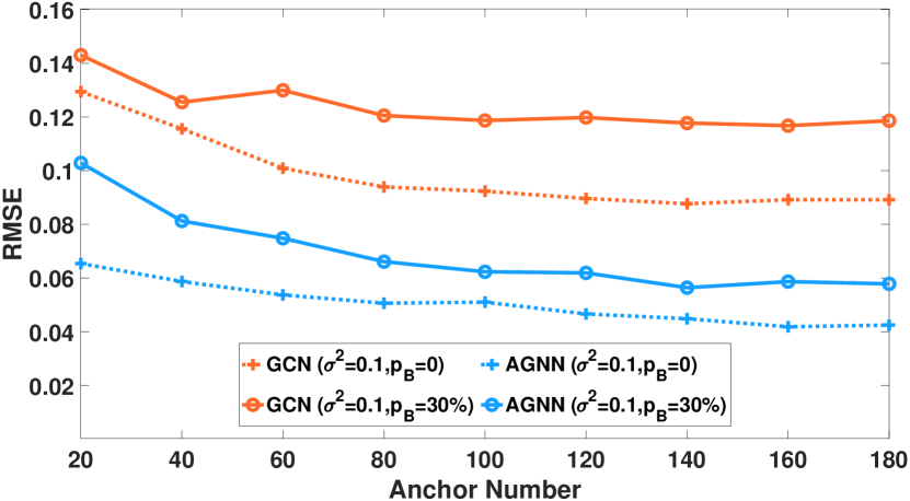
Subsequently, we focus on the performance of our proposed GNN-based methods, which perform relatively well in Tab. II. We explore localization error by varying from to with a stepsize of under two distinct noise conditions, presenting the results in Fig. 5. Two key observations can be drawn from these results. 1) Firstly, AGNN consistently achieves significantly lower RMSE for all values compared to the GCN-based method. Surprisingly, even under a 30% NLOS noise condition, AGNN consistently outperforms GCN in the scenario exclusively influenced by LOS noise, showcasing its efficacy in threshold learning and the feasibility of model expressiveness. 2) Secondly, as increases, both AGNN and GCN tend to converge towards their respective performance lower bounds. Notably, the lower bound of AGNN consistently surpasses that of GCN, especially under NLOS noise conditions. This finding suggests that AGNN is particularly well-suited for scenarios affected by NLOS noise.
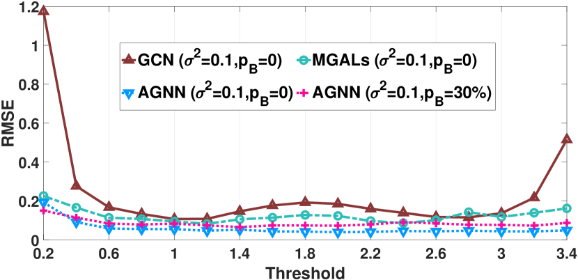
To comprehensively investigate the impact of the threshold, , on localization performance, we conduct an experiment systematically exploring the RMSE of GNN-based models across a range of , as depicted in Fig. 6. Here, ”MGALs” denotes a model constructed solely using two graph attention layers from Sec. IV-D, under the adjacency matrix determined by the manually-set threshold. For AGNN, the threshold here is the initial threshold employed for coarse-grained neighbor selection. Three key observations can be drawn from these results. 1) Firstly, Both MGALs and AGNN constantly achieve lower RMSE values compared to the GCN-based approach utilizing a constant aggregation weight. This underscores the effectiveness of learned aggregation weights through the attention mechanism in Sec. IV-D. 2) Secondly, akin to MGALs, AGNN exhibits initially low localization error. As increases, MGALs’ localization error experiences fluctuations, while AGNN’s error decreases rapidly and maintains consistently at a low level. This indicates that for AGNN, the graph attention layer plays a crucial role in ensuring localization accuracy when the initial threshold is set to a small value. While is relatively large, AGNN begins to leverage ALM, which allows for further refinement of the coarse-grained neighbor sets, thereby enhancing the accuracy of localization. 3) Lastly, AGNN demonstrates consistently low localization errors in two distinct noise environments across different values for , which underscores the robustness of AGNN-II under diverse noise conditions.
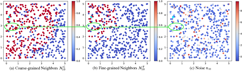
Furthermore, we also investigate the attention mechanism’s role in neighbor selection within AGNN by presenting scatter heatmaps of the coarse-grained neighbor set and the fine-grained neighbor set for the -th node in Fig. 7 (a) and (b). Nodes forming neighboring relationships with the -th node are highlighted in red, while others are displayed in blue. In Fig. 7 (c), a heatmap illustrates additive noise, , between the -th node and all others, transitioning from blue to red with increasing noise. Comparing Fig. 7 (a) and (b), we observe that neighbors omitted by the fine-grained set predominantly fall into two categories: those located at a relatively large distance from the -th node and those in close proximity but with relatively large noise. Specifically, the green circle represents nodes close to the -th node, including some within but not in . Examining the corresponding green region in Fig. 7 (c), we observe that the nodes omitted in exhibit relatively higher noise levels, with the additive noise ranging between . This observation underscores the effective refinement of the coarse-grained neighbor sets by the attention mechanism in AGNN, resulting in enhanced localization precision.
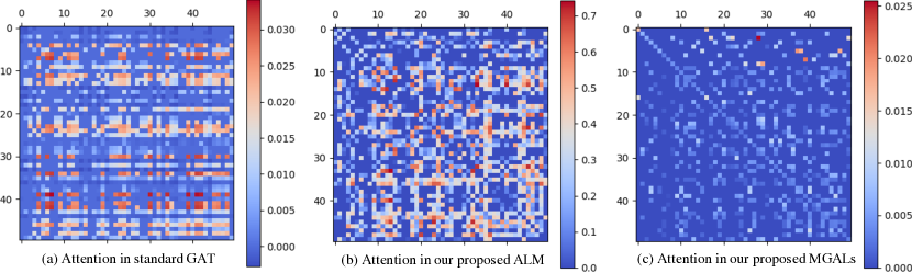
As detailed in Section V-A, we have established the dynamic attention property in both the proposed ALM and MGALs. To validate this, we compare attention scores for nodes with indices in the dataset among the standard GAT, ALM, and MGALs (first layer), as depicted in Fig. 8. Three key observations emerge. 1) For the standard GAT, as in Fig.8 (a), attention scores in each row have larger values at fixed columns, suggesting a consistent order in assigning weights to neighboring sets, indicating a static attention property. It’s noteworthy that in Sec.V-A, for clarity, we assume a neighboring set that includes all nodes. In practice, due to varying neighboring sets for each node, Fig. 8 (a) may have cases where attention scores should be large but are zero due to the node not being in the neighboring set. 2) The attention scores of ALM and MGALs for each node, as seen in Fig. 8 (b) and (c), lack a consistent order within their neighboring sets, indicating the dynamic attention property of ALM and MGALs. 3) In the comparison between Fig.8 (b) and (c), the attention scores of ALM exhibit symmetry, whereas those of MGALs do not. This is because the learned attention scores in ALM, as described in Eq.(13), are distance-aware and require symmetric property.
| Node | GCN | AGNN | MLP | LS | ECM | SDP |
| 500 | 3.24 | 5.23 | 2.33 | 32.47 | 82.85 | 1587 |
| 1000 | 5.82 | 14.66 | 3.94 | 89.92 | 353.4 | xxxx |
| 10000 | 707 | 1872 | 212 | xxxx | xxxx | xxxx |
In addition to accuracy, real-world applications demand prompt responses. Table III presents the computational times of various methods. Notably, the proposed GNN-based methods exhibit significantly reduced training times compared to traditional model-driven approaches. Particularly, for a network with 500 nodes, MLP, GCN, and AGNN only require several seconds, whereas model-driven methods incur substantially higher computational costs, reaching up to 1587s for SDP. Furthermore, it’s noteworthy that the computational time for the proposed GNN-based methods only exhibits a modest increase when doubling the number of nodes in the network. This scalability attribute underscores the efficiency of the proposed methods in large-scale scenarios. Especially, for super-large-scale networks, the proposed GNN-based methods exhibit a superior capability compared to traditional methods, exemplified by the case of where the GNN-based methods remain computationally affordable, while the traditional methods become impractical at such a scale. These results collectively suggest that the proposed GNN-based methods not only achieve high accuracy but also offer a prospective solution for large-scale network localization with efficient computational performance, making them suitable for real-world deployment.
VII Conclusion
In this paper, we mainly focus on the localization problem in large-scale wireless networks. Firstly, we have proposed a GCN-based data-driven method for robust large-scale network localization in mixed LOS/NLOS environments with manually defined graph structure. Furthermore, two types of AGNN models are proposed to autonomously learn the graph structure and then can achieve higher localization accuracy than the GCN-based model. Numerical results have shown that the proposed method is able to achieve substantial improvements in terms of localization accuracy, robustness and computational time, in comparison with both MLP and various benchmark methods. Additionally, we demonstrate that the proposed AGNN models have dynamic attention property and more flexible signal denoising property than GCN model, enhancing their suitability for dynamic network environments.
References
- [1] W. Yan, D. Jin, Z. Lin, and F. Yin, “Graph Neural Network for Large-Scale Network Localization,” in ICASSP 2021-2021 IEEE International Conference on Acoustics, Speech and Signal Processing (ICASSP). IEEE, 2021, pp. 5250–5254.
- [2] T. N. Kipf and M. Welling, “Semi-Supervised Classification with Graph Convolutional Networks,” in International Conference on Learning Representations (ICLR), Toulon, France, April 2017.
- [3] W. Hamilton, Z. Ying, and J. Leskovec, “Inductive Representation Learning on Large Graphs,” in Advances in neural information processing systems (NeurIPS), 2017, pp. 1024–1034.
- [4] P. Veličković, G. Cucurull, A. Casanova, A. Romero, P. Lio, and Y. Bengio, “Graph Attention Networks,” in International Conference on Learning Representations (ICLR), 2017.
- [5] K. Xu, W. Hu, J. Leskovec, and S. Jegelka, “How Powerful Are Graph Neural Networks,” in International Conference on Learning Representations (ICLR), 2019.
- [6] A. Ortega, P. Frossard, J. Kovačević, J. M. Moura, and P. Vandergheynst, “Graph Signal Processing: Overview, Challenges, and Applications,” Proceedings of the IEEE, vol. 106, no. 5, pp. 808–828, 2018.
- [7] F. Gama, A. G. Marques, G. Leus, and A. Ribeiro, “Convolutional Neural Network Architectures for Signals Supported on Graphs,” IEEE Transactions on Signal Processing, vol. 67, no. 4, pp. 1034–1049, 2018.
- [8] K. C. Dzmitry Bahdanau and Y. Bengio, “Neural Machine Translation by Jointly Learning to Align and Translate,” International Conference on Learning Representations, 2015.
- [9] A. W. Yu, D. Dohan, M.-T. Luong, R. Zhao, K. Chen, M. Norouzi, and Q. V. Le, “QANet: Combining Local Convolution with Global Self-Attention for Reading Comprehension,” in International Conference on Learning Representations, 2018.
- [10] A. Vaswani, N. Shazeer, N. Parmar, J. Uszkoreit, L. Jones, A. N. Gomez, Ł. Kaiser, and I. Polosukhin, “Attention Is All You Need,” Advances in neural information processing systems, vol. 30, 2017.
- [11] N. Patwari, A. O. Hero, M. Perkins, N. S. Correal, and R. J. O’Dea, “Relative Location Estimation in Wireless Sensor Networks,” IEEE Transactions on Signal Processing, vol. 51, no. 8, pp. 2137–2148, Aug 2003.
- [12] F. Yin, C. Fritsche, F. Gustafsson, and A. M. Zoubir, “EM-and JMAP-ML Based Joint Estimation Algorithms for Robust Wireless Geolocation in Mixed LOS/NLOS Environments,” IEEE Transactions on Signal Processing, vol. 62, no. 1, pp. 168–182, 2013.
- [13] A. Simonetto and G. Leus, “Distributed Maximum Likelihood Sensor Network Localization,” IEEE Transactions on Signal Processing, vol. 62, no. 6, pp. 1424–1437, 2014.
- [14] F. Yin, C. Fritsche, F. Gustafsson, and A. M. Zoubir, “TOA-Based Robust Wireless Geolocation and Cramér-Rao Lower Bound Analysis in Harsh LOS/NLOS Environments,” IEEE transactions on signal processing, vol. 61, no. 9, pp. 2243–2255, 2013.
- [15] H. Wymeersch, J. Lien, and M. Z. Win, “Cooperative Localization in Wireless Networks,” Proceedings of the IEEE, vol. 97, no. 2, pp. 427–450, 2009.
- [16] J. Costa, N. Patwari, and A. Hero, “Distributed Weighted-Multidimensional Scaling for Node Localization in Sensor Networks,” ACM Transactions on Sensor Networks, vol. 2, no. 1, pp. 39–64, 2006.
- [17] P. Biswas, T. Lian, T. Wang, and Y. Ye, “Semidefinite Programming Based Algorithms for Sensor Network Localization,” ACM Transactions on Sensor Networks, vol. 2, no. 2, pp. 188–220, May 2006.
- [18] P. Tseng, “Second-Order Cone Programming Relaxation of Sensor Network Localization,” SIAM Journal on Optimization, vol. 18, no. 1, pp. 156–185, 2007.
- [19] A. Ihler, J. W. Fisher, R. L. Moses, and A. S. Willsky, “Nonparametric Belief Propagation for Self-Localization of Sensor Networks,” in IEEE Journal on Selected Areas in Communications, 2005.
- [20] D. Jin, F. Yin, C. Fritsche, F. Gustafsson, and A. M. Zoubir, “Bayesian cooperative localization using received signal strength with unknown path loss exponent: Message passing approaches,” IEEE Transactions on Signal Processing, vol. 68, pp. 1120–1135, 2020.
- [21] S. Marano, W. M. Gifford, H. Wymeersch, and M. Z. Win, “NLOS Identification and Mitigation for Localization Based on UWB Experimental Data,” IEEE Journal on Selected Areas in Communications, vol. 28, no. 7, pp. 1026–1035, Sep. 2010.
- [22] F. Yin, C. Fritsche, D. Jin, F. Gustafsson, and A. M. Zoubir, “Cooperative Localization in WSNs Using Gaussian Mixture Modeling: Distributed ECM Algorithms,” IEEE Transactions on Signal Processing, vol. 63, no. 6, pp. 1448–1463, 2015.
- [23] H. Chen, G. Wang, Z. Wang, H. C. So, and H. V. Poor, “Non-Line-of-Sight Node Localization Based on Semi-Definite Programming in Wireless Sensor Networks,” IEEE Transactions on Wireless Communications, vol. 11, no. 1, pp. 108–116, 2012.
- [24] D. Jin, F. Yin, M. Fauß, M. Muma, and A. M. Zoubir, “Exploiting Sparsity for Robust Sensor Network Localization in Mixed LOS/NLOS Environments,” in IEEE International Conference on Acoustics, Speech and Signal Processing (ICASSP), 2020, pp. 5915–5915.
- [25] D. Jin, F. Yin, A. M. Zoubir, and H. C. So, “Exploiting Sparsity of Ranging Biases for NLOS Mitigation,” IEEE Transactions on Signal Processing, vol. 69, pp. 3782–3795, 2021.
- [26] F. Yin, Z. Lin, Q. Kong, Y. Xu, D. Li, S. Theodoridis, and S. R. Cui, “FedLoc: Federated Learning Framework for Data-Driven Cooperative Localization and Location Data Processing,” IEEE Open Journal of Signal Processing, vol. 1, pp. 187–215, 2020.
- [27] H. Ning, H. Wang, Y. Lin, W. Wang, S. Dhelim, F. Farha, J. Ding, and M. Daneshmand, “A survey on the metaverse: The state-of-the-art, technologies, applications, and challenges,” IEEE Internet of Things Journal, 2023.
- [28] Y. Qi, H. Kobayashi, and H. Suda, “Analysis of wireless geolocation in a non-line-of-sight environment,” IEEE Transactions on wireless communications, vol. 5, no. 3, pp. 672–681, 2006.
- [29] R. Zekavat and R. M. Buehrer, Handbook of Position Location: Theory, Practice and Advances. John Wiley & Sons, 2011, vol. 27.
- [30] P. Ramachandran, B. Zoph, and Q. V. Le, “Searching for Activation Functions,” in International Conference on Learning Representations (ICLR), 2018.
- [31] L. Bottou, “Large-Scale Machine Learning with Stochastic Gradient Descent,” in Proceedings of 19th International Conference on Computational Statistics. Springer, 2010, pp. 177–186.
- [32] D. P. Kingma and J. Ba, “Adam: A Method for Stochastic Optimization,” in International Conference on Learning Representations (ICLR), 2014.
- [33] A. Sandryhaila and J. M. Moura, “Discrete Signal Processing on Graphs: Frequency Analysis,” IEEE Transactions on Signal Processing, vol. 62, no. 12, pp. 3042–3054, 2014.
- [34] F. Gama, E. Isufi, G. Leus, and A. Ribeiro, “Graphs, Convolutions, and Neural Networks: From Graph Filters to Graph Neural Networks,” IEEE Signal Processing Magazine, vol. 37, no. 6, pp. 128–138, 2020.
- [35] F. Wu, T. Zhang, A. H. d. Souza Jr, C. Fifty, T. Yu, and K. Q. Weinberger, “Simplifying Graph Convolutional Networks,” in International Conference on Learning Representations (ICLR), 2019.
- [36] U. A. Brody, S. and E. Y., “How Attentive Are Graph Attention Networks?” in International Conference on Learning Representations (ICLR), 2022.
- [37] X. Wu, A. Ajorlou, Z. Wu, and A. Jadbabaie, “Demystifying oversmoothing in attention-based graph neural networks,” arXiv preprint arXiv:2305.16102, 2023.
- [38] K. Hornik, “Approximation capabilities of multilayer feedforward networks,” Neural networks, vol. 4, no. 2, pp. 251–257, 1991.
- [39] J. Bruna, W. Zaremba, A. Szlam, and Y. LeCun, “Spectral networks and deep locally connected networks on graphs,” in ICLR, 2014.
- [40] M. Defferrard, X. Bresson, and P. Vandergheynst, “Convolutional neural networks on graphs with fast localized spectral filtering,” NeurIPS, vol. 29, 2016.
VIII Appendix
VIII-A Proof of Theorem 2
Let’s consider a graph . This graph comprises transformed node representations, denoted as . Suppose is any node mapping.
We introduce a function , defined as follows:
| (26) |
Further, we define a continuous function , which matches at precisely specific inputs: , when . For all other inputs , assumes any values that preserve its continuity.
Note that is formulated for ease of proof. As our goal is for the graph attention layer’s scoring function to approximate the mapping at a finite set of points, we need to approximate at specific points. Although is discontinuous, is continuous, facilitating the use of the universal approximation theorem. By approximating , effectively approximates at our specified points. We only require to match at specific points . Beyond these points, ’s values are flexible, as long as its continuity is maintained.
Therefore, for every node and every , we have:
| (27) |
If we concatenate the input vectors and define the graph attention layer’s scoring function based on the concatenated vector , then according to the universal approximation theorem, can approximate for any compact subset of .
Hence, for any sufficiently small (where ), there exist parameters and such that for every node and every :
| (28) |
Owing to the increasing monotonicity of the function, this implies:
| (29) |
This show that our proposed graph attention layer possesses dynamic attention, as it assigns the highest attention score to any neighbor node depending on the concatenated feature vector.
VIII-B Proof of Theorem 3
The expression for the attention coefficient in ALM, as defined in Eq. (13), can be reformulated as follows:
| (30) |
where . Here, the notation represents the -th column vector or the -th element of a matrix or vector.
Based on the decomposition of the summation in Eq. 30, we focus on the -th term, denoted as . Let , and then sort in ascending order to obtain the corresponding indices of the node sorting, denoted as . Assuming the scalar is positive, then for every , we have:
| (31) |
If the scalar is negative, then for every , we have:
| (32) |
It is evident that the maximum value of is not fixed but rather depends on and . Thus, , as the attention coefficient in the summation of for the -th term, exhibits a dynamic attention property.
Similar conclusions can be drawn for the remaining terms, wherein the difference arises due to the varying orders of determined by the specific values of and , which further ensures the dynamic attention property.
VIII-C Proof of Theorem 4
The complexity analysis of the -th graph convolutional layer can be segmented into two components: Eq. (4) and Eq. (5).
First, we consider the operation described in Eq. (4), which entails a matrix product involving a sparse adjacency matrix and a dense representation matrix. Specifically, the -th row of can be expressed as follows:
| (33) |
Here, the computation of demands in terms of time complexity. Given that , the overall time complexity for Eq. (4) becomes .
Secondly, for the matrix multiplication between two dense matrices, as seen in Eq. (5), the well-known time complexity is .
In summary, the time complexity of the -th graph convolutional layer can be succinctly expressed as .
VIII-D Proof of Theorem 5
The proof of Theorem 5 comprises two distinct parts, pertaining to the time complexity analysis of ALM and the k-th graph attention layer within the MGALs.
The primary computational complexity within ALM arises from the calculation of attention coefficients, as articulated in Eq. (13). Firstly, we compute for every , which necessitates . Subsequently, for each edge , we compute using the pre-computed and , incurring a time complexity of . Finally, computing the results of the linear layer adds an additional . In summary, the time complexity of ALM amounts to .
The computational complexity of the k-th graph attention layer within MGALs can be broken down into several components. Initially, we compute Eq. (20) for every , demanding . Subsequently, we calculate for every using the pre-obtained , which incurs a time complexity of . Further, computing the results of the linear layer takes . Finally, we compute Eq.(22) for every , requiring . Consequently, the time complexity for the k-th graph attention layer within MGALs is given by .
By systematically analyzing each component, we have established the respective time complexities for ALM and the k-th graph attention layer within MGALs as outlined above.