Modular Neural Networks for Time Series Forecasting:
Interpretability and Feature Selection using Attention

Abstract

Multivariate time series have many applications, from healthcare and meteorology to life science. Although deep learning models have shown excellent predictive performance for time series, they have been criticised for being black-boxes or non-interpretable. This paper proposes a novel modular neural network model for multivariate time series prediction that is interpretable by construction. A recurrent neural network learns the temporal dependencies in the data while an attention-based feature selection component selects the most relevant features and suppresses redundant features used in the learning of the temporal dependencies. A modular deep network is trained from the selected features independently to show the users how features influence outcomes, making the model interpretable. Experimental results show that this approach can outperform state-of-the-art interpretable Neural Additive Models (NAM) and variations thereof in both regression and classification of time series tasks, achieving a predictive performance that is comparable to the top non-interpretable methods for time series, LSTM and XGBoost.

1 Introduction

Deep Neural Networks (DNNs) are a popular method for analysing multivariate time series as they can identify hidden data patterns to ensure an accurate approximation [15], and overcome the linearity challenges that are often associated with traditional time series models such as support vector machines and auto regressive models [44]. Transformer-based models and attention mechanisms have recently been shown to achieve high accuracy in forecasting [9, 16] due to their ability to capture long-term dependencies in data, and their efficiency in processing the data, thus allowing for faster training and inference.

However, in real life domains, users demand more from DNNs than effective predictive performance alone. They want the decisions to be interpretable. The area of explainable AI (XAI) has gained traction as it sought to make DNNs more transparent and understandable to humans in order to increase trust in AI systems. XAI research can be divided into post-hoc and ante-hoc. Many post-hoc approaches have been proposed in recent years, with varying results focused on the approximation and evaluation of the underlying models. In this paper, we focus on ante-hoc approaches following the general idea that the provision of modular networks may offer high performance with interpretability. Ante-hoc approaches are often criticised for their lack of flexibility in that a prescribed module may not be suitable to any given application domain, producing the same trade-off between accuracy and interpretability as seen in post-hoc XAI [31]. Our goal is to develop modular but flexible interpretable DNNs that do not require post-hoc XAI, but can still outperform interpretable traditional methods, such as decision trees [12], whilst matching the performance of non-interpretable models.

This paper introduces Attention Modular Networks (AMN), which can handle both time series forecasting and classification tasks. AMN also provides both feature importance and the exact depiction of how a given feature of the model contributed to model outcome, offering interpretability in the same way that NAMs do. In addition, AMN outperforms NAMs and other state-of-the-art interpretable methods. AMN matches the performance of classic non-interpretable approaches. These results are obtained, considering the four data sets used in this paper, by introducing two novel ideas: (i) the use of an attention mechanism for feature selection, and (ii) re-using the attention weights to bootstrap the training of each feature-specific network for the final prediction, as follows.

2 Related Work

2.1 DNN for Multivariate Time Series Forecasting

Recurrent networks are very popular for analysing multivariate time series problems due their ability to remember past inputs and use them to inform future decisions. Many variants have been proposed over the years, like Recurrent Neural Network (RNN) [13], Long Short-Term Memory (LSTM) [20], Bidirectional LSTM (BLSTM) [35], and Gated Recurrent Unit (GRU) [8]. LSTM and GRU were introduced to overcome the gradient vanishing problem faced by an RNN [4], and in turn have shown to be useful for learning long-term dependencies [11]. Since LSTM has a more complex architecture than GRU, training a GRU requires fewer computational resources. On the other hand, LSTMs have shown to be more capable than GRU in handling large amount of data and have more parameters that can be adjusted to optimise their performance, making them a popular choice for analysing multivariate time series problems across a variety of real-life applications [21, 22, 34, 37]. Despite their ability at handling time series data however, they are not interpretable.

2.2 Interpretable Additive Models

There have been a number of different ante-hoc methods proposed for time series analysis, including Shaplets [14, 42], Symbolic Aggregate Approximation [33, 36], and Fuzzy Logic [28, 41]. Often, these methods address either regression or classification tasks, but not both. More importantly, these methods do not scale well with large datasets. A recent interest in adding interpretability to Generalised Additive Models (GAM) [19] has demonstrated that they are capable of learning both time series prediction and classification problems. In addition, such GAM variants, such as Neural Additive Model (NAM) [1], GA²M [27], Neural Interaction Transparency [38], and Neural Basis Model [30], are computationally efficient and can handle large datasets.

For instance, NAM [1], an interpretable variant of GAM, learns a linear combination of a family of interpretable neural networks that each is assigned to learn a single input feature. This family of networks are trained jointly using backpropagation and have the ability to learn arbitrarily complex shape functions. The impact of a feature on prediction can then be interpreted and visualised by plotting its corresponding shape function, since it does not rely on other features. As such, this visualisation is the exact depiction of how NAM arrived at a prediction. NAM is also capable of learning non-linear relationships in the data, making it an attractive choice for many real-world applications. Unfortunately, the predictive performance of these models does not match that of more popular, non-interpretable time series models; for this reason, they cannot simply be regarded as a substitute for non-interpretable models [12]. The Scalable Polynomial Additive Model (SPAM) approach [12] builds on NAM by providing higher-order interactions between features and is intended to replace non-interpretable models for large scale data due to its high performance. The main difference between SPAM and NAM is that the intelligibility of SPAM arises from using tensor rank decomposition of polynomials, so higher-order feature interactions can be learned to provide an inherently interpretable model. However, the explanations provided by SPAM cannot be readily visualised in the same manner as NAM and, as such, they are harder to interpret than NAM.

2.3 Attention Mechanism for Feature Selection

Recently attention mechanisms have been used as a way to provide interpretability as they provide insight into which features of the data contribute the most to the prediction. In terms of multivariate time series analysis, using attention mechanism with recurrent-based network has been a popular choice [9, 16, 29]. However, these methods only focus on either classification [9, 16] or regression tasks [29]. Temporal Fusion Transformer (TFT) [24] was introduced recently for a multi-horizon forecasting task with added interpretability such as visualising the persistent temporal pattern with attention mechanism. Another example is the Interpretable Temporal Attention Network (ITANet) [46] for COVID-19 forecasting and inferring the importance of government interventions. However, TFT faces a limitation that it needs a large amount of data to achieve a good predictive performance [43]; whereas ITANet is only able to provide feature importance as an explanation.

Feature selection has been demonstrated to be an effective approach for preparing high-dimensional data when performing a variety of machine learning tasks [18]. Several different architectures that incorporate an attention mechanism into DNNs for feature selection have been proposed recently, such as Attention-based Feature Selection (AFS) [18], Multiattention-based Feature Selection (MFS) [6], and TabNet [2]. In AFS, several attention mechanisms are utilised in an attention module to select features directly from the input, then a learning module where different DNNs can be used to learn the selected inputs. MFS share a similar architecture with AFS, the main difference between the two is that two different attention mechanisms are employed in the attention module where one is learning the variable attention and the other one is learning the temporal attention in the inputs. However, in both AFS and MFS, interpretability only exists in the attention module and not the learning module where the actual learning takes place. TabNet is an interpretable sequential multi-step processing network and introduced a sequential attention mechanism for feature selection. Although TabNet achieved state-of-the-art results compared to non-interpretable DNN models, the explanations provided only considers feature attributions.

3 Attention Modular Networks (AMN)

We introduce an interpretable modular network that uses attention for feature selection of time series. AMN is in the same category as interpretable additive models such as NAM and SPAM, and it is an extension of NAM. Although NAM is able to provide both feature importance and depictions of model decision as explanations, its performance is not comparable to non-interpretable models. Despite the fact that SPAM claims to benchmark such models, it offers only features importance explanations. AMN performs better than NAM and provides explanations like NAM which are easier to understand than those of SPAM. To achieve this, AMN uses attention for feature selection inspired by AFS and MFS. Learning only the most salient features has been shown to be a useful method for improving interpretability and allocating learning capacity more effectively [6, 18]. Interpretability in AMN is provided by the attention mechanism along with the computation of the time series prediction being simply a linear combination of interpretable modular networks. Predictive performance is improved by identifying relevant features and ignoring features that do not contribute to the output.

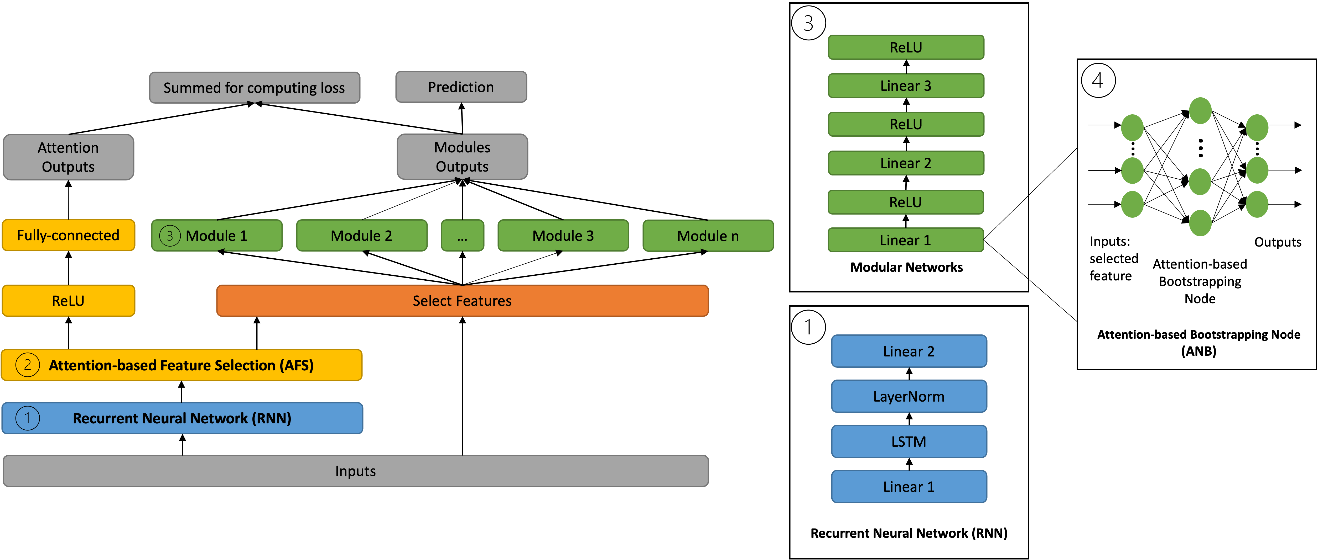
Figure 1: Attention Modular Networks (AMN architecture). AMN consists of three components: a Recurrent Neural Network (RNN) \small1⃝, an Attention-based Feature Selection (AFS) \small2⃝, and a group of interpretable Modular Networks \small3⃝. The Attention-based Node Bootstrapping (ANB) \small4⃝ in each module’s first layer is weighted by the AFS’s attention weights.

3.1 Recurrent Neural Network

Pre-processed inputs are first processed in the RNN component. LSTM is proposed to be used as the main learner, as shown in Fig. 1. The RNN component is responsible for learning the time-dependencies in the input data. In the hidden layer of an LSTM network, there are some special units called memory cells that are recurrently connected, as well as their corresponding gate units, namely input gate, forget gate, and output gate [20]. The final hidden state ($h_{t}$) is calculated through a series of gating mechanism as in the set of (1), where $x_{t}$ is the input vector at current timestep $t$, and $i_{t}$, $f_{t}$, and $o_{t}$ are the input, forget, and output gates, respectively. $w_{x}$ and $w_{h}$ are the weights and $b$ is the bias. Furthermore, $\sigma$ denotes the sigmoid function, $\tanh$ is the hyperbolic tangent function, and $\bigodot$ is the element-wise product. Finally, $c_{t}$ represents the cell state and $s_{t}$ is a newly created vector during computation, which decides if the new information should be stored in the cell state or not.

$$\left\{\begin{aligned} f_{t}&=\sigma(w_{x}x_{t}+w_{h}h_{t-1}+b)\\ i_{t}&=\sigma(w_{x}x_{t}+w_{h}h_{t-1}+b)\\ s_{t}&=\tanh(w_{x}x_{t}+w_{h}h_{t-1}+b)\\ c_{t}&=f_{t}\bigodot c_{t-1}+i_{t}\bigodot s_{t}\\ o_{t}&=\sigma(w_{x}x_{t}+w_{h}h_{t-1}+b)\\ h_{t}&=\tanh(c_{t})\bigodot o_{t}\end{aligned}\right.$$ (1)

A common issue when training an RNN, e.g., LSTMs, is the vanishing or exploding gradients problem, i.e., when gradients become too small or big during training, making it difficult to update the network weights. Furthermore, LSTMs suffer from unstable hidden representations due to the highly dynamic nature of their state updates [3]. To avoid this, layer normalisation [3] is applied to the LSTM outputs to alleviate the gradient-related problems [3], as it re-centers and re-scales the activation in the LSTM layer to have zero mean and unit variance, hence making it easier to propagate gradients through the network.

3.2 Attention-based Feature Selection (AFS)

Vaswani et al. [40] introduced a generalised definition for an attention function, describing it as mapping a query, $\bm{Q}\in\mathbb{R}^{N\times d_{q}}$, and a set of key-value pairs, $\bm{K}\in\mathbb{R}^{N\times d_{k}}$, $\bm{V}\in\mathbb{R}^{N\times d_{v}}$ to an output, where $d_{q}$, $d_{k}$, and $d_{v}$ are dimensions of $\bm{Q}$, $\bm{K}$, and $\bm{V}$, respectively. The attention mechanism then scales $\bm{V}$ based on relationships between $\bm{K}$ and $\bm{Q}$, usually through scaled dot-product [40], such that:

$$\mathrm{Attention}(\bm{Q},\bm{K},\bm{V})=\mathrm{softmax}(\frac{\bm{Q}\bm{K^{T}}}{\sqrt{d_{k}}})\bm{V}$$ (2)

On (2), a single attention function is performed with potentially large dimensional $d_{q}$, $d_{k}$, and $d_{v}$. In the initial proposal of Vaswani et al. [40] for a Multi-head attention mechanism, each head attends to an input sub-sequence, so as to reduce the computational complexity of (2) and $\bm{Q}$, $\bm{K}$, $\bm{V}$ can be linearly projected with different projections to $d_{q}$ and $d_{v}$ dimensions, respectively.

However, we employ the Attention Mechanism in AMN as a feature selection tool, which means that we cannot have each head attend to an input sub-sequence, because as Lim et al. [24] suggested, using the attention weights of the Multi-head Attention alone cannot be indicative of importance of a particular feature, given that different $\bm{V}$s are used in each head. To overcome this, Attention-based Feature Selection (AFS) is proposed. Instead of having each attention head attending to some smaller sub-sequences of the input, the Multi-head attention is modified so each attention head computes the attention weight of each input feature independently. It is worth to note here that making this modification does not change the mathematical concept of the original Multi-head Attention mechanism – the modification is merely to how the attention is applied.

Let us denote the final output of the RNN component as $R$. In AFS, the attention function in (3) is applied to each $R_{i}$, where each $AH_{i}$ is an attention head of the Multi-head Attention, and where $\bm{Q}\bm{W}^{Q}_{i}\in\mathbb{R}^{d_{q}\times d_{v}}$, $\bm{K}\bm{W}^{K}_{i}\in\mathbb{R}^{d_{k}\times d_{v}}$, and $\bm{V}\bm{W}^{V}_{i}\in\mathbb{R}^{d_{q}\times d_{v}}$ are the projections of attention head-specific weights for $\bm{Q}$, $\bm{K}$, $\bm{V}$, respectively. Finally, in (4), $\bm{W}_{AH}\in\mathbb{R}^{(AH\cdot d_{v})\times d_{q}}$ linearly combines concatenated outputs from all attention heads, thus completing the Multi-head attention function.

$$AH_{i}=\mathrm{Attention}(\bm{Q}\bm{W}^{Q}_{i},\bm{K}\bm{W}^{K}_{i},\bm{V}\bm{W}^{V}_{i})$$ (3)

$$\mathrm{MultiHead}(\bm{Q},\bm{K},\bm{V})=[AH_{1},AH_{2},...,AH_{n}]\bm{W}_{AH}$$ (4)

$\bm{W}_{AH}$ is then averaged to compute the average attention weights for each $R_{i}$ by applying a feature-wise pooling operation. The final output of the AFS component is obtained by applying the $\mathrm{softmax}$ function to the computed average attention weights, $\text{Attn}(R_{i})$, for normalisation:

$$\bm{F_{i}}=\mathrm{softmax}(\text{Attn}(R_{i}))$$ (5)

Based on $F_{i}$, top $n$ features can then be selected from the original input. In AMN, $n$ can be set either directly or as a hyper-parameter. To ensure the gradients of $\bm{F}$ can be propagated properly and be reused in the subsequent component (discussed in detail in the following section), $\bm{F}$ are sent through a Rectified Linear Unit (ReLU) and a fully-connected layer so the loss of RNN-AFS components can be calculated (discussed in detail in section 3.5).

3.3 Modular Networks

The idea of modularity has been researched as early as the 1980s and adopted in neural information processing in the late 1990s. It was recognised then [5] that traditional Artificial Neural Networks are black-box in nature and Modular Networks are more interpretable and explainable. An Modular Networks follows the divide-and-conquer principle [39] and is inspired by the important biological fact that neurons in human brains are sparsely connected in a clustered and hierarchical fashion, rather than completely connected [5]. In an Modular Networks, several smaller simple NNs are used, where each NN focuses on a different part of the same problem and their outputs are combined together into one final solution for the entire network. In this way, using an Modular Networks allows complex learning problems to be simplified [39], as well as to mimic human thinking to resolve these large-scaled complex problems [5].

Each module in the Modular Networks component of AMN consists of a single selected input feature trained independently, so that the impact of each feature on the prediction is independent of other features. Thus, this component methodologically belong to the GAM family, following (6), where $y$ is the target variable, $g$ is the link function, $\bm{x}=x_{1},x_{2},...,x_{n}$ is the input (or the selected input in the case of AMN), and each $f_{i}$ is a univariate shape function with $\mathbb{E}(f_{i})=0$.

$$g(\mathbb{E}(y))=\beta+f_{1}(x_{1})+f_{2}(x_{2})+\cdots f_{n}(x_{n})$$ (6)

The Modular Networks component rendering the AMN interpretable because each univariate shape function is parameterised by a neural network through a series of linear transformations, as done with NAM. The main difference between AMN and NAM is that each feature is initially weighted using the attention weights $\bm{F}$, which will be shown to improve predictive performance considerably. To achieve this, we introduce Attention-based Node Bootstrapping (ANB) to each module (see Fig. 1\small4⃝) to learn the weights based on the inputs factored by the attention weights and shifted by a bias. For each module, Xavier Initialisation [17] initialises the biases (to zeros) and weights at each layer. The previously-computed attention weights for the selected features, $\bm{F}$, are then multiplied by the initialised weights, $\bm{W}_{\text{init}}$, as in (7). Finally, the ReLU activation function is applied to each ANB for each scalar input $x$, as shown in (8). In practice, ANB is applied in the first layer of each module (Linear 1 in Fig. 1\small3⃝), so each $\bm{F_{i}}$ can be used directly. These individual networks are then trained jointly with the RNN and AFS components using back-propagation, below.

$$\bm{W}_{\text{mod}_{i}}=\bm{W}_{\text{init}_{i}}*\bm{F_{i}}$$ (7)

$$ANB(x)=\text{ReLU}((x-b)*\bm{W}_{\text{mod}})$$ (8)

3.4 Learning Rate Scheduler

Since the AMN strongly resembles the Transformer architecture, we are employing the Cosine Annealing learning rate (LR) warm-up scheduler [26] to further accelerate convergence, stabilise the training, and improve generalisation for the Adam optimisation algorithms [25]. Rather than setting the LR as a constant or in a decreasing order, the LR warm-up technique gradually increases the LR from zero to the specified LR in the first few training iterations. This is particularly important for adaptive optimisation algorithms, such as Adam, because these algorithms use the bias correction factors that can lead to a higher variance in the first few training iterations. Furthermore, layer normalisation techniques applied in the RNN component can also lead to very high gradients during the first iterations.

3.5 Loss Functions

To ensure the network gradients flow through all components of the AMN and improve the convergence of the AMN during training, the RNN-AFS and Modular Networks components are trained jointly, with each one aiming to minimise the Mean Squared Error Loss ($\frac{1}{N}\sum(y_{i}-\tilde{y_{i}})^{2}$) in the case of regression tasks, and a Binary Cross-Entropy with Logits Loss ($-\frac{1}{N}\sum_{i=1}^{N}(y_{i}*log(\tilde{y_{i}})+(1-y_{i})*log(1-\tilde{y_{i}}))$) in the case of classification tasks, where $y$ is the target value, $\tilde{y_{i}}$ is the predicted value, and $N$ is the number of data points. The sum of the two losses give the loss function for the AMN to minimise:

$$\text{Loss}_{\text{AMN}}=\text{Loss}_{\text{RNN-AFS}}+\text{Loss}_{\text{mod}}$$ (9)

4 Experimental Results

AMN’s predictive performance was evaluated on two regression and two classification tasks against state-of-the-art interpretable and non-interpretable methods:

• Neural Additive Model (NAM) [1]. AMN is an extension of this work and the objective of AMN is to maintain interpretability but improve upon its predictive performance.

• Scalable Polynomial Additive Model (SPAM) [12]. Although SPAM considers feature interactions and thus performs better than NAM, only feature importance and not feature curves can be provided by SPAM as explanations.

• Long Short-Term Memory (LSTM) [20]. Stand-alone LSTM offers a baseline for evaluating multivariate time series models; however, it is not interpretable.

• Extreme Gradient Boosted Trees (XGBoost). This is another popular non-interpretable standard approach Both NAM and SPAM are compared with XGBoost and therefore we do too.

Table 1: Test set average results comparison of AMN with other methods on four data sets for time series regression and classification. Means and standard deviations are reported from 5 random trials with optimal hyper-parameters. Appendix A.1 describes the hyper-parameter optimization for each task. Details about the data sets are provided in Appendix A.2. OtiReal [10] is used to predict future hearing aid usage, Air [45] predicts future particulate matter values (PM_2.5), EEG [32] predicts eyes-open or closed states, and Rain in Australia (Weather) predicts if it will rain tomorrow or not. For regression tasks, lower results are better ($\downarrow$). For classification tasks, higher results are better ($\uparrow$).

Regression $\downarrow$ Classification $\uparrow$ SMAPE MASE WAPE Speed Accuracy F1 AUC Speed Air AMN $\mathbf{0.2640}^{**}$ $\mathbf{0.1654}^{**}$ $\mathbf{0.1637}^{**}$ 1,198.10 EEG AMN $\mathbf{0.8203^{*}}$ $\mathbf{0.8131^{*}}$ $\mathbf{0.8203^{*}}$ 24.28 NAM $0.5221^{*}$ $0.4166^{*}$ $0.4206^{*}$ 3,598.02 NAM $0.5430^{**}$ $0.0115^{**}$ $0.5020^{**}$ 136.56 SPAM 0.5231 0.2765 0.2778 1,571.26 SPAM $0.5000^{*}$ $0.0159^{*}$ $0.5002^{*}$ 115.61 XGBoost(50) $0.2704^{**}$ $0.1704^{**}$ $0.1706^{**}$ 15.42 XGBoost(5) $0.6959^{**}$ $0.6169^{*}$ $0.6824^{**}$ 0.02 LSTM $0.2935^{*}$ $0.1774^{**}$ $0.1772^{**}$ 1,289.57 LSTM $0.5000^{**}$ 0.2667 $0.5^{**}$ 53.53 OtiReal AMN $0.2105^{*}$ $1.4829$ $0.0806^{**}$ 96.32 Weather AMN $\mathbf{0.8518}^{**}$ $0.5157^{*}$ $0.6791^{**}$ 1,192 NAM $0.8543^{*}$ $12.3317$ 0.6661 238.95 NAM $0.8169^{**}$ 0.2442 $0.5687^{*}$ 1,552.91 SPAM 0.2951 2.3075 $0.1249^{*}$ 119.73 SPAM $0.8369^{**}$ 0.4305 $0.6444^{*}$ 1,231.40 XGBoost(100) $0.9574^{**}$ $\mathbf{1.0840}^{**}$ $0.6846^{**}$ 1.29 XGBoost(5) $0.8473^{*}$ $\mathbf{0.5508}^{*}$ $\mathbf{0.7009}^{*}$ 20.67 LSTM $\mathbf{0.1809}^{*}$ 1.2694 $\mathbf{0.0666}^{*}$ 92.77 LSTM $0.8419^{**}$ $0.4592^{*}$ $0.6509^{**}$ 664.46

Interpretable model. Non-interpretable model.
^(∗∗): Variance across experiments is $<0.01$. ^(∗): Variance across experiments is $<0.05$.
Note: The number in parentheses after XGBoost is the optimal number of trees; XGBoost is considered to be non-interpretable when the number of trees exceeds 10.

Experimental results are summarised in Table 3. The top 10 features are selected for all data sets (i.e. we use Modular Networks with 10 modules). AMN outperforms both interpretable models NAM and SPAM in both regression and classification tasks . This is the case for every standard metric used, namely Symmetric Mean Absolute Percentage Error (sMAPE), Mean Absolute Scaled Error (MASE), Weighted Absolute Percentage Error (WAPE), Accuracy, F1 score, and Area Under the Curve (AUC).

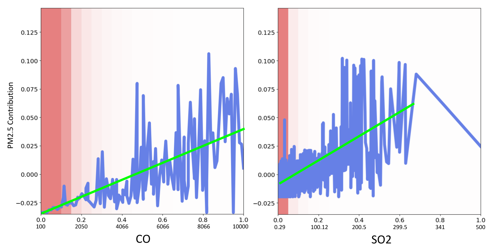
(a) Air data set. Showing graphs (shape functions) learned by AMN at predicting future PM_2.5 value given Carbon Monoxide and Sulfur Dioxide concentration. The shape function plot for CO shows an overall positive correlation (highlighted by the superimposed green line) with large variation. Similarly for SO2 there is a positive correlation until the sudden drop when SO2 exceeds 320 $\mu g/mg^{3}$. Notice how simply sampling the input to the LSTM to obtain such correlations would not be informative or feasible in practice with an increased number of input variables.

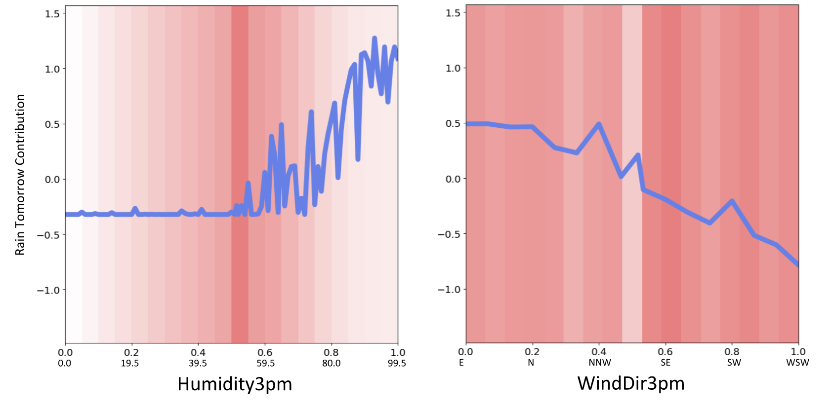
(b) Weather data set. The graphs learned by AMN predict whether it will rain tomorrow given Humidity and Wind Direction. The shape function plot for Humidity3pm shows that humidity from 60 to 99% at 3pm today will likely lead to rain tomorrow. The start of the upward trend of the contribution of humidity occurs in a region of high data density. The plot for WindDir3pm shows higher chances of rain when there is a northerly wind compared with lower chances of rain when the wind direction changes to a more southerly wind.

Figure 2: NAM-style explanations for selected features learned by Modular Networks. Network outputs are shown on the y-axis. Feature values are shown on the x-axis (normalised values above and actual values below). The blue line represents the learned shape function. Normalised data densities are shown using the red bars, the darker the red, the more data there is in that region.

As Table 3 shows, AMN also matches the performance of non-interpretable models (OtiReal and Weather data sets), or outperforms them (Air and EEG data sets). A visual representation of regression results is useful when there is a discrepancy in results depending on the choice of metric, as in the case of the OtiReal results. Visualisations in Appendix A.3 show that both AMN and LSTM perform better than XGBoost at capturing the underlying trend in the data with a lower SMAPE and WAPE. In Air, the prediction results of AMN are the best aligned with the test set. NAM generally performs worse in a classification task than in a regression task, achieving only 1.2% and 24.4% F1 score in the EEG and Weather data sets, respectively. By utilising AFS in the architecture, AMN overcomes this limitation of NAM and produces the best results of all approaches on EEG, while matching the performance of XGBoost with the best results on Weather. This is discussed further in section 5.1.

Besides evaluating the prediction results, we have also noted the computational time for all experiments. Although the computation time of XGBoost is the shortest for all experiments, Table 3 shows that the computation time of AMN is one of the shortest amongst the DNN models, and sometimes even shorter than a simple LSTM model (Air and EEG).

As an interpretable model, AMN is able to provide explanatory graphs showing the influence of selected features on model prediction. A selection of such graphs is shown in Fig. 2, with further analyses of the explanations provided for each data set in Appendix B. As with NAM, the interpretability of AMN comes from visualising the shape functions of each module network. Since each selected feature is learned independently by a module, the shape functions show the exact depiction of a module’s contribution to a prediction, e.g., prediction of particulate matter PM_2.5 as a function of carbon monoxide CO, $PM2.5=f(CO)$ with a positive correlation. The plots also show the corresponding normalised data density in intensities of red for each selected feature. Notice how in Fig. 2(b) the contribution of SO2 decreases linearly when the value of SO2 exceeds 320 $\mu g/mg^{3}$. This should warrant further investigation as the plot shows that there is insufficient data (with a lighter shade of red) when SO2 values exceed 100 $\mu g/m^{3}$. With these plots, the effect of CO and SO2 on PM_2.5 can be further investigated, hopefully to produce a better understanding of the model and drive model intervention and improvement.

5 Additional Experiments

5.1 Effectiveness of AFS

As observed in the Table 3, NAM tends to perform worse in the classification tasks than regression tasks. Therefore, to further validate the effectiveness of the proposed AFS, the effect of changing the number of features to be selected by the AFS is examined. Using one of the classification dataset - Weather, the test accuracy are compared across two experiments $n=10$ (reported in the Results) and $n=21$ (all available features in the inputs). Optimal hyper-parameters for the Weather dataset selected during hyper-tuning are used for both experiments, and trained for 100 epochs with the Adam optimiser and early call-backs to avoid over-fitting.

The results shows the test accuracy of the $n=10$ experiment is more than double of the test accuracy of the $n=21$ experiment ($n=10$: 0.5-, $n=21$: 0.22). This experiment shows that the proposed AFS is effective at improving the performance of AMN.

5.2 Effectiveness of ANB

Table 2: Test loss comparison between different RNN network configuration and different Weighted Linear Layer in the Air dataset.

Configuration	Test Loss
LSTM + ANB	0.0070
GRU + ANB	0.0072
BLSTM + ANB	0.0216
LSTM + Linears	0.0216
GRU + Linears	0.0251
BLSTM + Linears	0.0338
LSTM + ExU	0.0513
GRU + ExU	0.0591
BLSTM + ExU	0.1334

In this additional experiment, three different types of Recurrent-based networks are experimented with. These are GRU, LSTM, and BLSTM. Furthermore, first layer in each module (Linear 1 in \small3⃝ of Fig. 1) is changed to a standard Linear layer (with no modified hidden unit) to test the effectiveness of ANB as proposed in section 3.3. As the Modular Networks component is inspired by NAM, ANB (see (8)) in the first layer of each module is replaced by ExU, as in NAM [1]. For this experiment, all models are trained with the same hyper-parameters with 128 batch size, 0.002 learning rate, 128 hidden RNN units, 64 and 32 hidden units for the second and third linear layers in each module respectively (i.e., Layer 2 and Layer 3 in \small3⃝ of Fig. 1), and trained for 100 epochs with the Adam optimiser and early call-backs to avoid over-fitting.

Using the Air dataset, Table 2 shows that the LSTM+ANB combination achieved the lowest loss compared to all experiments. Also, any combination with ExU performed worse than its Linears and ANB counterparts. As can be seen, the proposed ANB is effective at improving the performance of AMN, with LSTM+ANB, GRU+ANB, and BLSTM+ANB being the best performers.

6 Conclusion and Future Work

A novel interpretable modular neural network using attention for feature selection, named AMN, was introduced and evaluated in this paper. It has two main innovations: Attention-based Feature Selection (AFS) and Attention-based Node Bootstrapping (ANB). In AFS, Multi-head Attention is modified to select the most relevant features from the original input. ANB acts as a bridge between AFS and each module of the interpretable Modular Networks by weighing each selected feature with its corresponding attention weights.

The goal of AMN was to improve the model’s predictive performance compared to NAM and yet retain interpretability. Experiments have shown that AMN not only outperforms NAM on all metrics (and its variation SPAM), but it can match the predictive performance of state-of-the-art non-interpretable models LSTM and XGBoost, outperforming the state-of-the-art in some cases.

AFS, MFS, and TabNet share some similarities with our proposed AMN; however, AMN is distinct from them because attention weights are learned from a recurrent-based network in AMN so as to obtain a prior temporal knowledge and used for feature selection, and AMN offers a flexibility in using different variants of recurrent-based networks. Lastly, we consider AMN to be more closely related to architectures with modularity, such as additive models. A common assumption of such modules such as GAM and NAM is feature independence. This has been proved to be too strong an assumption in certain areas of application such as time series, as indicated by the poor predictive performance of such models in the experiments reported in this paper. AMN tackles this problem by using AFS for feature selection during training. Variations of NAM on the other hand, such as SPAM, seek to tackle the same problem by allowing interaction terms. This, however, may increase the complexity of the explanations provided for these models. As future work, we shall evaluate this and other trade-offs, such as the number of modules to use, in practice, since it is likely that the answers will depend on the characteristics of the specific application domain and associated expert evaluation.

Limitations of the results reported in this paper include the lack of experiments using multi-class time series classification. In comparison with SPAM, a given application may require the use of higher-order feature interaction, not available in AMN. We shall investigate the possibility of an attention mechanism creating such features for implementation into a single network module. Finally, we shall continue to investigate the practical value of the explanations provided, how they may inform model intervention, and the interactions that may exist between attention-based explanations of recurrent networks and interpretable modular networks.

Appendix A Experiment Details

A.1 Optimal Hyper-parameters

The optimal hyper-parameters for each model for each dataset are listed below. Hyper-parameters are hyper-tuned using Ray-tune with the validation set. More specifically, Asynchronous Successive Halving Algorithm scheduler [23] is used for better parallelism, with the Optuna search algorithm.

Table 3: Optimal Hyper-Parameters

Hyper-parameters OtiReal Air EGG Weather AMN Initial Learning Rate 0.0130 0.0008 0.0021 0.0003 Dropout rate in the RNN 0.0318 0.0349 8.6209$e^{5}$ 0.1992 Dropout rate in the Modular Networks 0.1450 0.0142 0.0005 0.8378 Dropout rate in the final output 0.0339 0.0513 0.0011 0.1851 Batch Size 256 64 512 64 Number of hidden unit in the RNN 256 64 64 1,026 Number of hidden units in the Modular Networks [256, 128] [256, 128] [32, 16] [512, 256] NAM Learning Rate 0.0065 0.0122 0.0007 0.0002 Dropout Rate 0.4875 0.0405 0.0107 0.0218 Batch Size 64 512 256 256 Hidden Sizes [128, 64] [512, 256] [64, 32] [256, 128] SPAM Learning Rate 0.268 0.1902 0.0009 Dropout Rate 0.1072 0.0265 0.0590 Batch Size 64 256 64 LSTM Learning Rate 0.0260 0.0082 0.7330 0.0369 Dropout rate 0.1153 0.0567 0.2340 0.1285 Batch Size 256 64 128 64 Number of hidden unit 64 128 128 256 XGBoost Number of estimators 1,000 200 50 1,000 Max Depths 100 50 5 5 Subsample 0.2605 0.8069 0.3804 0.3191 Learning Rate 0.3370 0.7600 2.8467$e^{5}$ 0.4725

A.2 Datasets Description

Table 4: Datasets Description

Name OtiReal Air EEG Weather Source [10] [45] [32] http://www.bom.gov.au/climate/data/ Instances 24,736 420,768 14,892 137,910 Features 16 16 14 21 Class Distribution - - 1: 0.82 1: 0.26 Feature Type Mixed Mixed Continuous Mixed Top Features 10 10 10 10

Real-world longitudinal and observational hearing aid data are collected from patients signed up for the HearingFitness^TM feature with the Oticon ON^TM remote control app on the Oticon Open Hearing Aids (Oticon A/S, Smørum, Denmark). Christensen et al. [10] extracted a sampled data OtiReal of 98 in-market users between June-December 2019 that contains no personal information characterising the patients to preserve privacy. OtiReal dataset contains sound data concerning the acoustic environment detected by the hearing aids and logged by the connected smart-phones. These sound data include Sound Pressue Level (SPL), Modulation Index (MI), Signal-to-Noise Ratio (SNR), and Noise Floor (NF), all measured in a broadband frequency range of 0-10kHz in decibel units. Besides the sound data, hearing aid usage is also calculated from the timestamps when the sound data are collected. The task is then to predict future daily hearing aid usage.

Air quality is another popular domain that needs time series analysis. In the Beijing Multi-Site Air-Quality (Air) dataset [45], 7 years of meteorological data along with 4 years of $\text{PM}_{2.5}$ data of Beijing at 36 monitoring sites were collected. $\text{PM}_{2.5}$ refers to the fine particulate matter (PM) concentration in the air with aerodynamic diameter of less than 2.5 $\mu m$. The tasks is to predict future $\text{PM}_{2.5}$ values.

In the EEG Eye State (EEG) dataset, continuous electroencephalogram (EEG) measurement are collected from the Emotive EEG Neuroheadset [32]. The duration of the EEG measurement is 119 seconds, and eye state (e.g., whether the eyes are closed or open) are detected by a camera during EEG measurement and added to the dataset manually later, where 1 indicates eye-closed and 0 indicates eye-open. The task is a binary one to classify eye state based on the EEG measurement.

Another binary classification dataset is the Rain in Australia (Weather) dataset, which contains 10 years of daily weather observations drawn from a number of weather stations in Australia. Features include location, minimum/maximum temperature, amount of rainfall, and wind gust. The task is to predict whether or not it will rain tomorrow.

A.3 Prediction Results Visualisation

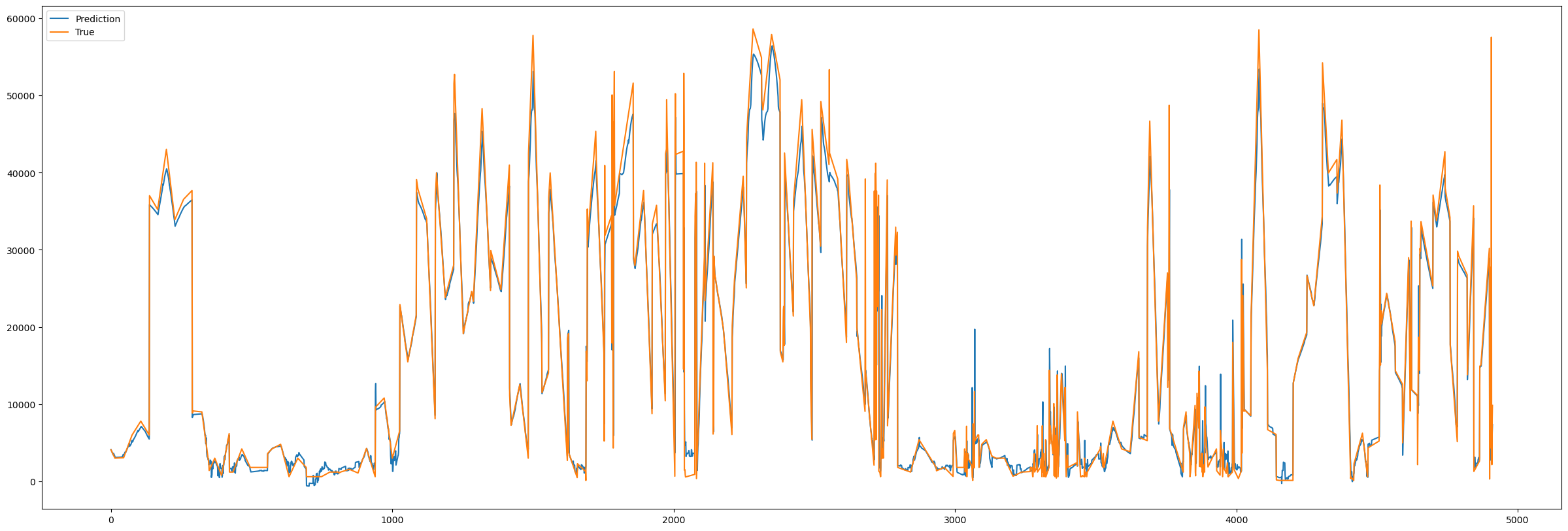
(a) AMN

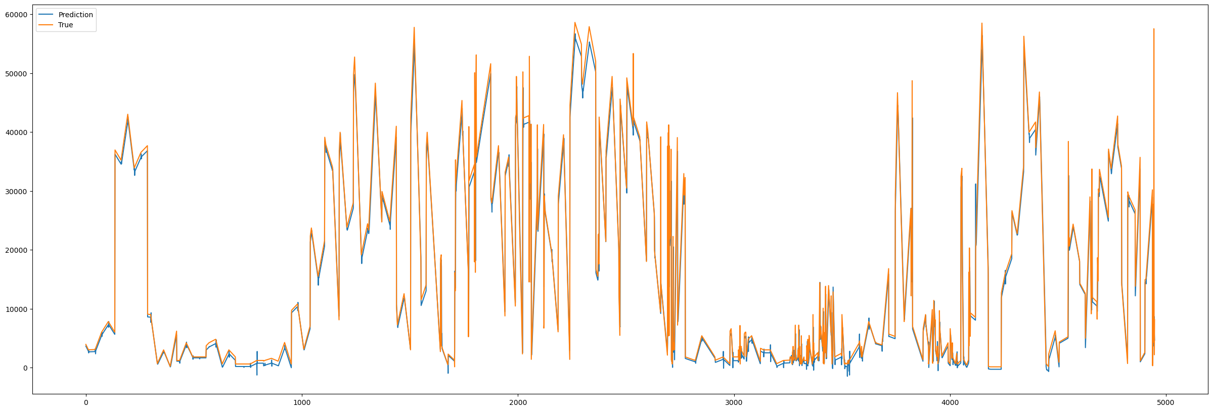
(b) LSTM

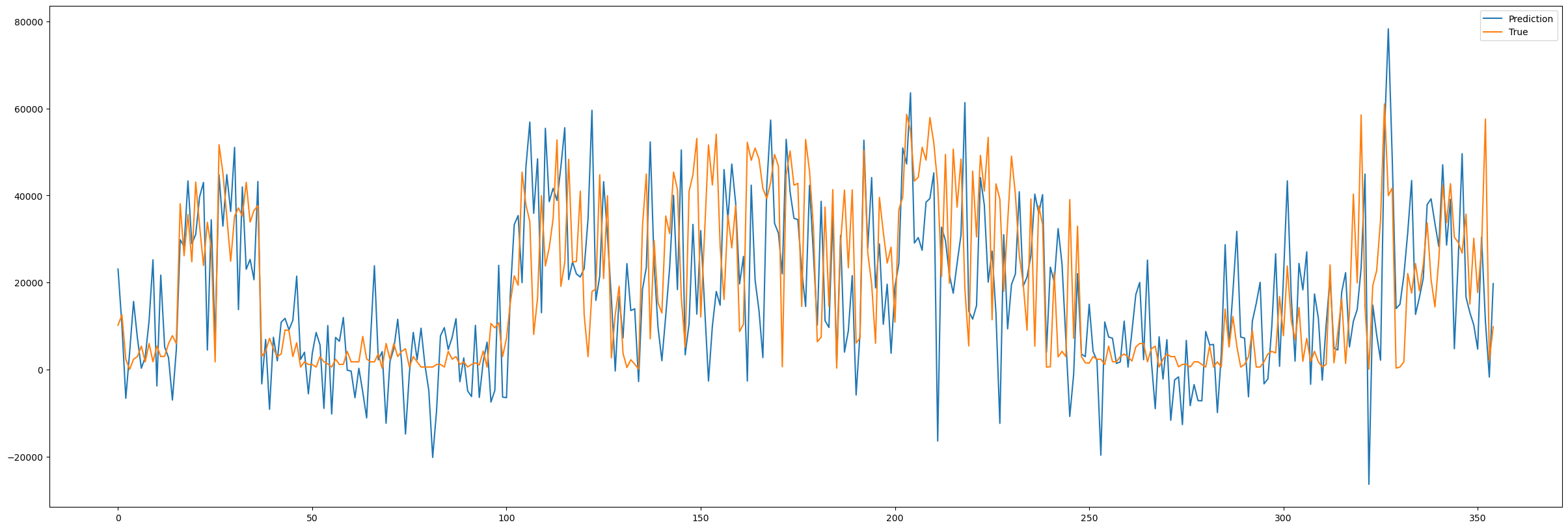
(c) XGBoost

Figure 3: Prediction Visualisations, where x-axis represents predicted timesteps and y-axis represents feature values. Note: data are pre-processed differently for XGBoost. More specifically, XGBoost supports missing values by default, whereas missing values are interpolated for training with AMN and LSTM.

As discussed in section 4, AMN and LSTM achieved the lowest SMAPE and WAPE but did not achieve a good MASE result. While XGBoost achieved the lowest MASE error, its SMAPE and WAPE errors are one of the worst when comparing with other models. Both SMAPE and WAPE are percentage-based error estimators and focus on the accuracy of percentage errors, whereas MASE assess the ability of a model relative to a simple benchmark model. Therefore, a visual inspection of the prediction results would be helpful to decide which model performed the best in the OtiReal dataset. While metrics are essential for quantitative evaluation, the ultimate goal is to achieve predictions that align with the underlying pattern and behaviour in the data.

As Figure 3 shows, both AMN and LSTM are better at capturing the pattern and trend in the OtiReal dataset than XGBoost as the predicted values are much better aligned to the true values. The figure also shows that the magnitude of the true/target values vary significantly in the OtiReal dataset and both SMAPE and WAPE are better at comparing models in this situation than MASE.

Appendix B Model Explanations

B.1 Explanations for OtiReal Dataset

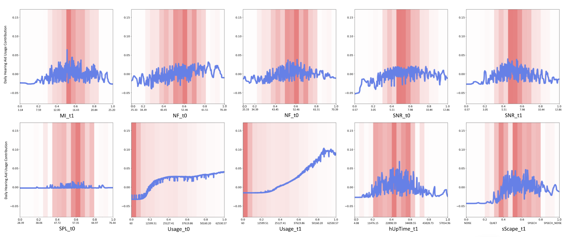
Figure 4: OitReal Graphs learned by AMN in predicting future hearing aid usage (regression) on the OtiReal dataset. These plots show top 10 features selected by the AFS component in the AMN, where selected features with normalised and original values are on the x-axis, and daily future hearing aid usage prediction contribution are on the y-axis. In OtiReal, two timesteps of data are transformed and used as inputs, such that we are using data at $t_{i}$ and $t_{i+1}$ to predict hearing aid usage at $t_{i+2}$.

The shape plots for the acoustic variables (e.g., MI, NF, and SNR) follow a similar pattern in contributing to the model prediction, where patients with median MI, NF, and SNR values sensed by the hearing aids tend to use their hearing aids more in the future. In terms of Modulation Index (MI), patients will be more likely to use their hearing aids more in the future if MI values sensed by the hearing aids are around 15 decibels, and are less likely to use their hearing aids more in the future if MI values sensed by the hearing aids are either less than 10 or more than 23 decibels. For Noise Floor (NF), if the the hearing aids sense the NF value at around 50 decibels, then these patients will be more likely to use their hearing aids more in the future. For Signal-to-Noise Ratio (SNR), patients will be more likely to use their hearing aids more in the future if SNR values sensed by the hearing aids are around 6 decibels. Hearing Aid Up Time (hUpTime) also follows a similar pattern with these acoustic variables where if the hearing aids have been activated for around 23,000 seconds (or 6.3 hours), then these patients will be most likely to use their hearing aids more in the future.

Comparing with other acoustic variables, Sound Pressure Level (SPL) does not contribute much to predicting future hearing aid usage. This would warrant a further investigation with the audiologists as MI and SNR are derived from SPL, such that MI is the difference between peak and valley detector of the SPL and SNR is the difference between the valley detector and the immediate SPL.

The shape plots for Usage show, as expected, patients with higher daily hearing aid usage are more likely to have higher future daily hearing aid usage and patients with lower daily hearing aid usage are more likely to have lower future daily hearing aid usage. The difference in the shape function (blue line) in Usage_t0 and Usage_t1 shows that the maximum contribution to future hearing aid usage for Usage_t0 is around 0.05, whereas the maximum contribution for Usage_t1 is around 0.1. This means that patients are more likely to have an even higher future daily hearing aid usage if they use their hearing aids for a sufficiently long period in a day continuously (for at least 2 days in this case). The most rapid increase in future hearing aid usage contribution at Usage_t0 occurs when hearing aid usage is above 10,000 seconds (or 3 hours), this means this is the minimum hearing aid usage that a patient needs to have to be able to have a higher future hearing aid usage. Whereas the most rapid increase in future hearing aid usage contribution at Usage_t1 occurs when hearing aid usage is above 20,000 seconds (or 6 hours).

The Soundscape (sScape) classifies momentary sound environment into four categories by a proprietary hearing aid algorithm using MI, SNR, and SPL values. Its plot shows that if the soundscape is at noise or quiet setting, then these patients are less likely to use their hearing aids more in the future, whereas if the soundscape is at speech setting, then these patients are more likely to use their hearing aids more in the future. This could be an interesting observation to the audiologists as this might show that those patients who are active and use their hearing aids to assist their hearing loss will tend to continuously use their hearing aids in the future, and on the other hand those patients who might not be familiar with their hearing aids or not actively use their hearing aids are less likely to continuously use their hearing aids in the future.

B.2 Explanations for Air Dataset

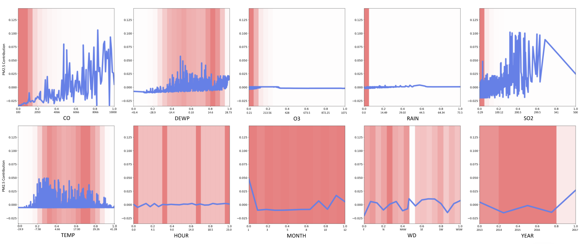
Figure 5: Air Graphs learned by AMN in predicting future PM_2.5 values (regression) on the Air dataset. These plots show top 10 features selected by the AFS component in the AMN, where selected features with normalised and original values are on the x-axis, and future PM_2.5 values prediction contribution are on the y-axis.

In this section, explanations for CO and SO2 are excluded as they are already included in section 4.

The plot for Dew Point Temperature (DEWP) shows that when DEWP is at around 0 degree Celsius, predicted future PM_2.5 values tend to be the highest. The contribution of DEWP towards predicting future PM_2.5 values then drops at around 7 degree Celsius and increases again at around 12 degree Celsius.

O3 Concentration (O3), Precipitation (RAIN), HOUR contribute almost nothing towards predicting future PM_2.5 values, and the contribution of O3 even becomes negative with high O3 values (e.g., high O3 leads to lower future PM_2.5 values).

The plot for Temperature (TEMP) shows that when temperature is in the range of -8 and 28 degrees Celsius, future PM_2.5 values are predicted to be the highest, whereas when the temperature is above 28 and below -8 degree Celsius, this will lead to a low future PM_2.5 values. This observation is in line with many literature studying correlation between PM_2.5 and season such that there is a negative correlation in summer and autumn and positive correlation in spring and winter [7]. The plot for MONTH also confirms this observation, such that future PM_2.5 values are predicted to be the highest in January, followed by November and September.

The plot for Wind Direction (WD) shows that future PM_2.5 values are predicted to be the lowest when there is a Eastern wind, and future PM_2.5 values are predicted to be the highest when the wind changes from a northerly to southerly wind (i.e., normalised value at around 0.5 on the x-axis). When the wind direction changes from Southwestern wind to West-southwestern wind, it is also likely leads to a lower future PM_2.5 value. Lastly, the plot for YEAR shows that more recent data (i.e., data from 2016 onward) have more impact on the model in predicting higher future PM_2.5 values. Whereas there is a drastic decrease in contribution of YEAR towards predicting future PM_2.5 values in the years between 2013 and 2014.

B.3 Explanations for EEG Dataset

Figure 6 shows that AF4, F4, F7, FC5, O1, O2, and T8 have almost no contribution towards AMN in predicting eye state from the EEG, and AF3 and P7 have minimal contribution towards the model prediction. This means that electrodes placed at these regions do not contribute much to AMN in predicting the eye state.

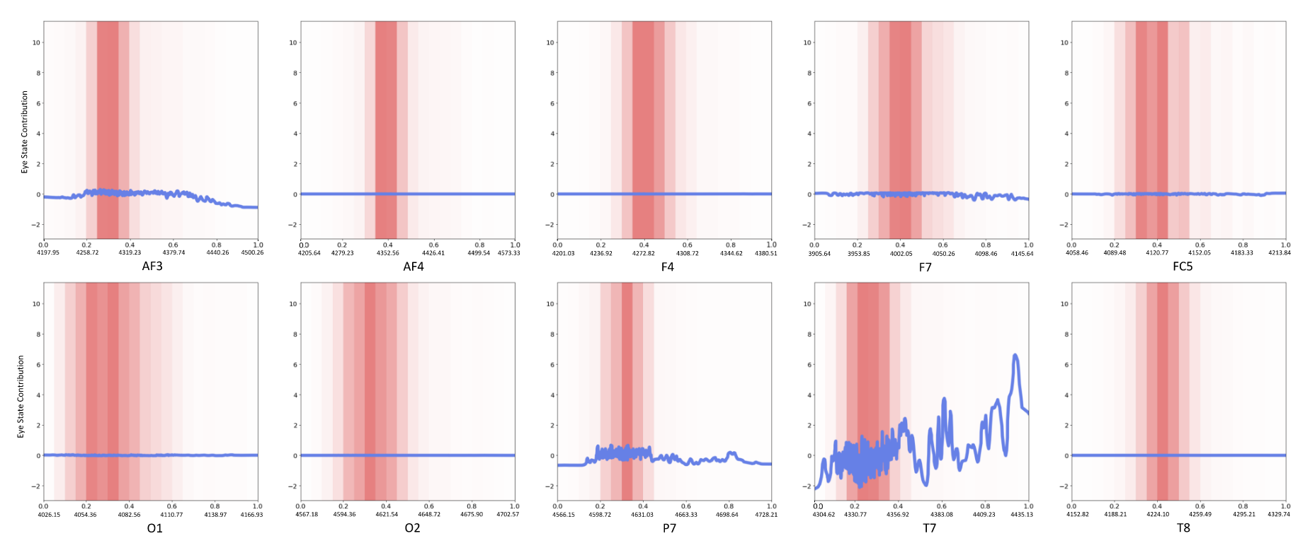
Figure 6: EEG Graphs learned by AMN in predicting eye state (classification) on the EEG dataset. These plots show top 10 features selected by the AFS component in the AMN, where selected features with normalised and original values are on the x-axis, and contribution towards the prediction are on the y-axis.

Figure 6 shows that the electrode placed on the T7 region is the most important one in predicting the eye state. Its plot shows that higher T7 values means it is more likely that the eyes are open (i.e., label 1), and lower T7 values means it is more likely that the eyes are closed (i.e., label 0). Interestingly, T7 is a feature that is neither the most correlated to the outcome nor the one with the highest multicollinearity. Meaning that AMN managed to capture the non-linear relationship in the underlying data.

B.4 Explanations for Weather Dataset

Figure 7: Weather Graphs learned by AMN in predicting whether it will rain tomorrow (classification) on the Weather dataset. These plots show top 10 features selected by the AFS component in the AMN, where selected features with normalised and original values are on the x-axis, and contribution towards the prediction are on the y-axis.

In this section, explanations for Humidity3pm and WindDir3pm are excluded as they are already included in section 4.

The plot for Cloud9am shows that this feature contributed nothing in AMN predicting whether or not it will rain tomorrow.

The plot for Evaporation shows that the relationship between Evaporation and future rain fall is rather complicated. This is as expected as although both evaporation and precipitation (rainfall) are connected within the water cycle, their relationship depends on several factors including global climate phenomena and local factors. Nevertheless, this shape plot would be helpful to meteorologists to discover the detailed pattern between Evaporation and Rain. For example, in this specific case, when Evaporation reaches 13mm, then this will most likely lead to rain tomorrow. This complicated relationship can also be observed with Pressure9am and Temp9am, and how atmospheric pressure and temperature affects the chance of raining the next day also depends on other factors.

The plot for Humidity9am follows a similar pattern to Humidity3pm, with a drastic increase in the chance of raining tomorrow when the humidity is above 60%. Therefore, when humidity at 9am is above 60%, it will most likely to rain tomorrow, and when humidity at 9am is less than 60%, it will most likely to not rain tomorrow.

The plot for Maximum Temperature (MaxTemp) shows that higher maximum temperature means there is a less chance of raining tomorrow, and there is a drop in chance of raining tomorrow when the maximum temperature is above 5 degree Celsius.

The plot for Rainfall shows that, as expected, the more rainfall detected on the recorded day, more likely to rain tomorrow. There is a drop in chance of raining tomorrow when rainfall detected on the recorded day is above 17mm, and this might warrant a further investigation with the meteorologist.

The plot for WindGustSpeed shows that when the speed of the strongest wind is at around 70km/h, it is more likely to rain tomorrow. The chance of raining tomorrow then drop when the speed of the strongest wind is above 70km/h. Whereas when the speed of the strongest wind is less than 49 km/h, it is more likely to not rain tomorrow.

References

- [1] R. Agarwal, L. Melnick, N. Frosst, X. Zhang, B. Lengerich, R. Caruana, and G.E. Hinton. Neural additive models: Interpretable machine learning with neural nets. Advances in Neural Information Processing Systems, 34, 2021.
- [2] S.O. Arik and T. Pfister. Tabnet: Attentive interpretable tabular learning. Proceedings of the AAAI Conference on Artificial Intelligence, 35:6679–6687, 8 2021.
- [3] J.L. Ba, J.R. Kiros, and G.E. Hinton. Layer normalization. arXiv:1607.06450, 7 2016.
- [4] Y. Bengio, P. Simard, and P. Frasconi. Learning long-term dependencies with gradient descent is difficult. IEEE Transactions on Neural Networks, 5:157–166, 3 1994.
- [5] T. Caelli, Ling G., and W. Wen. Modularity in neural computing. Proceedings of the IEEE, 87:1497–1518, 1999.
- [6] L. Cao, Y. Chen, Z. Zhang, and N. Gui. A multiattention-based supervised feature selection method for multivariate time series. Computational Intelligence and Neuroscience, 2021:1–10, 7 2021.
- [7] Ziyue Chen, Jun Cai, Bingbo Gao, Bing Xu, Shuang Dai, Bin He, and Xiaoming Xie. Detecting the causality influence of individual meteorological factors on local pm2.5 concentration in the jing-jin-ji region. Scientific Reports, 7:40735, 1 2017.
- [8] K. Cho, B. van Merrienboer, D. Bahdanau, and Y. Bengio. On the properties of neural machine translation: Encoder-decoder approaches. arXiv: 1409.1259, 9 2014.
- [9] K.S. Choi, S.H. Choi, and B. Jeong. Prediction of idh genotype in gliomas with dynamic susceptibility contrast perfusion mr imaging using an explainable recurrent neural network. Neuro-Oncology, 21:1197–1209, 9 2019.
- [10] Jeppe H. Christensen, Gabrielle H. Saunders, Michael Porsbo, and Niels H. Pontoppidan. The everyday acoustic environment and its association with human heart rate: evidence from real-world data logging with hearing aids and wearables. Royal Society Open Science, 8:rsos.201345, 2 2021.
- [11] J. Chung, C. Gulcehre, K. Cho, and Y. Bengio. Empirical evaluation of gated recurrent neural networks on sequence modeling. arXiv:1412.3555, 12 2014.
- [12] A. Dubey, F. Radenovic, and D. Mahajan. Scalable interpretability via polynomials. arXiv:2205.14108, 5 2022.
- [13] J.L. Elman. Finding structure in time. Cognitive science, 14:179–211, 1990.
- [14] Z. Fang, P. Wang, and W. Wang. Efficient learning interpretable shapelets for accurate time series classification. In 2018 IEEE 34th International Conference on Data Engineering (ICDE), pages 497–508. IEEE, 4 2018.
- [15] W. Gao, M. Aamir, A.B. Shabri, R. Dewan, and A. Aslam. Forecasting crude oil price using kalman filter based on the reconstruction of modes of decomposition ensemble model. IEEE Access, 7:149908–149925, 2019.
- [16] W. Ge, J-W. Huh, Y.R. Park, J-H. Lee, Y-H. Kim, and A. Turchin. An interpretable icu mortality prediction model based on logistic regression and recurrent neural networks with lstm units. AMIA … Annual Symposium proceedings. AMIA Symposium, 2018:460–469, 2018.
- [17] X. Glorot and Y. Bengio. Understanding the difficulty of training deep feedforward neural networks. In Yee Whye Teh and Mike Titterington, editors, Proceedings of the Thirteenth International Conference on Artificial Intelligence and Statistics, pages 249–256. {PMLR},, 5 2010.
- [18] N. Gui, D. Ge, and Z. Hu. Afs: An attention-based mechanism for supervised feature selection. Proceedings of the AAAI Conference on Artificial Intelligence, 33:3705–3713, 7 2019.
- [19] T. Hastie and R. Tibshirani. Generalized additive models. Statistical Science, 1, 8 1986.
- [20] S. Hochreiter and J. Schmidhuber. Long short-term memory. Neural computation, 9:1735–1780, 1997.
- [21] Y. Hua, Z. Zhao, R. Li, X. Chen, Z. Liu, and H. Zhang. Deep learning with long short-term memory for time series prediction. IEEE Communications Magazine, 57:114–119, 2019.
- [22] Y. Huang, C-H. Chen, and C-J. Huang. Motor fault detection and feature extraction using rnn-based variational autoencoder. IEEE Access, 7, 2019.
- [23] L. Li, K. Jamieson, A. Rostamizadeh, E. Gonina, M. Hardt, B. Recht, and A. Talwalkar. A system for massively parallel hyperparameter tuning. arXiv:1810.05934, 10 2018.
- [24] B Lim, S.O Arık, N Loeff, and T Pfister. Temporal fusion transformers for interpretable multi-horizon time series forecasting. International Journal of Forecasting, 37:1748–1764, 10 2021.
- [25] L. Liu, H. Jiang, P. He, W. Chen, X. Liu, J. Gao, and J. Han. On the variance of the adaptive learning rate and beyond. arXiv:1908.03265v4, 8 2019.
- [26] I. Loshchilov and F. Hutter. Sgdr: Stochastic gradient descent with warm restarts. arXiv:1608.03983, 8 2016.
- [27] Y. Lou, R. Caruana, J. Gehrke, and G. Hooker. Accurate intelligible models with pairwise interactions. In Proceedings of the 19th ACM SIGKDD international conference on Knowledge discovery and data mining, pages 623–631. ACM, 8 2013.
- [28] R.P. Paiva and A. Dourado. Interpretability and learning in neuro-fuzzy systems. Fuzzy Sets and Systems, 147:17–38, 10 2004.
- [29] L. Pantiskas, K. Verstoep, and H. Bal. Interpretable multivariate time series forecasting with temporal attention convolutional neural networks. In 2020 IEEE Symposium Series on Computational Intelligence (SSCI), pages 1687–1694. IEEE, 12 2020.
- [30] F. Radenovic, A. Dubey, and D. Mahajan. Neural basis models for interpretability. arXiv:2205.14120, 5 2022.
- [31] M.T. Ribeiro, S. Singh, and C. Guestrin. "why should i trust you?": Explaining the predictions of any classifier. In Proceedings of the 22nd ACM SIGKDD International Conference on Knowledge Discovery and Data Mining, pages 1135–1144. Association for Computing Machinery, 2016.
- [32] Oliver Roesler. Eeg eye state, 2013.
- [33] T. Rojat, R. Puget, D. Filliat, J. Del Ser, R. Gelin, and N. Díaz-Rodríguez. Explainable artificial intelligence (xai) on timeseries data: A survey. arXiv preprint arXiv:2104.00950, 4 2021.
- [34] H. Sak, A.W. Senior, and F. Beaufays. Long short-term memory recurrent neural network architectures for large scale acoustic modeling. In Proceedings of the Annual Conference of International Speech Communication Association (INTERSPEECH), 2014.
- [35] M. Schuster and K.K. Paliwal. Bidirectional recurrent neural networks. IEEE Transactions on Signal Processing, 45:2673–2681, 1997.
- [36] P. Senin and S. Malinchik. Sax-vsm: Interpretable time series classification using sax and vector space model. In 2013 IEEE 13th International Conference on Data Mining, pages 1175–1180. IEEE, 12 2013.
- [37] M.A.I. Sunny, M.M.S. Maswood, and A.G. Alharbi. Deep learning-based stock price prediction using lstm and bi-directional lstm model. In 2nd Novel Intelligent and Leading Emerging Sciences Conference (NILES), pages 87–92, 2020.
- [38] M. Tsang, H. Liu, S. Purushotham, P. Murali, and Y. Liu. Neural interaction transparency (nit): Disentangling learned interactions for improved interpretability. Advances in Neural Information Processing Systems, 31, 2018.
- [39] S. Varela-Santos and P. Melin. A new modular neural network approach with fuzzy response integration for lung disease classification based on multiple objective feature optimization in chest x-ray images. Expert Systems with Applications, 168:114361, 4 2021.
- [40] A. Vaswani, N. Shazeer, N. Parmar, J. Uszkoreit, L. Jones, A.N. Gomez, L. Kaiser, and I. Polosukhin. Attention is all you need. arXiv:1706.03762, 6 2017.
- [41] Z. Wang, W. Yan, and T. Oates. Time series classification from scratch with deep neural networks: A strong baseline. In 2017 International Joint Conference on Neural Networks (IJCNN), pages 1578–1585. IEEE, 5 2017.
- [42] L. Ye and E. Keogh. Time series shapelets. In Proceedings of the 15th ACM SIGKDD international conference on Knowledge discovery and data mining - KDD ’09, page 947. ACM Press, 2009.
- [43] H. Zhang, Y. Zou, X. Yang, and H. Yang. A temporal fusion transformer for short-term freeway traffic speed multistep prediction. Neurocomputing, 500:329–340, 8 2022.
- [44] P.G. Zhang. Time series forecasting using a hybrid arima and neural network model. Neurocomputing, 50:159–175, 1 2003.
- [45] S. Zhang, B. Guo, A. Dong, J. He, Z. Xu, and S.X. Chen. Cautionary tales on air-quality improvement in beijing. Proceedings of the Royal Society A: Mathematical, Physical and Engineering Sciences, 473:20170457, 9 2017.
- [46] B. Zhou, G. Yang, Z. Shi, and S. Ma. Interpretable temporal attention network for covid-19 forecasting. Applied Soft Computing, 120:108691, 5 2022.