1-Lipschitz Layers Compared: Memory, Speed, and Certifiable Robustness

Abstract

The robustness of neural networks against input perturbations with bounded magnitude represents a serious concern in the deployment of deep learning models in safety-critical systems. Recently, the scientific community has focused on enhancing certifiable robustness guarantees by crafting $1$-Lipschitz neural networks that leverage Lipschitz bounded dense and convolutional layers. Although different methods have been proposed in the literature to achieve this goal, understanding the performance of such methods is not straightforward, since different metrics can be relevant (e.g., training time, memory usage, accuracy, certifiable robustness) for different applications. For this reason, this work provides a thorough theoretical and empirical comparison between methods by evaluating them in terms of memory usage, speed, and certifiable robust accuracy. The paper also provides some guidelines and recommendations to support the user in selecting the methods that work best depending on the available resources. We provide code at github.com/berndprach/1LipschitzLayersCompared.

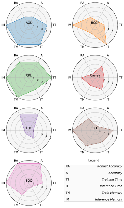
Figure 1: Evaluation of $1$-Lipschitz methods on different metrics. Scores are assigned from 1 (worst) to 5 (best) to every method based on the results reported in Sections 3 and 5.

1 Introduction

Modern artificial neural networks achieve high accuracy and sometimes superhuman performance in many different tasks, but it is widely recognized that they are not robust to tiny and imperceptible input perturbations [33, 3] that, if properly crafted, can cause a model to produce the wrong output. Such inputs, known as Adversarial Examples, represent a serious concern for the deployment of machine learning models in safety-critical systems [21]. For this reason, the scientific community is pushing towards guarantees of robustness. Roughly speaking, a model $f$ is said to be $\varepsilon$-robust for a given input $x$ if no perturbation of magnitude bounded by $\varepsilon$ can change its prediction. Recently, in the context of image classification, various approaches have been proposed to achieve certifiable robustness, including Verification, Randomized Smoothing, and Lipschitz bounded Neural Networks.

Verification strategies aim to establish, for any given model, whether all samples contained in a $l_{2}$-ball with radius $\varepsilon$ and centered in the tested input $x$ are classified with the same class as $x$. In the exact formulation, verification strategies involve the solution of an NP-hard problem [15]. Nevertheless, even in a relaxed formulation, [38], these strategies require a huge computational effort [37].

Randomized smoothing strategies, initially presented in [9], represent an effective way of crafting a certifiable-robust classifier $g$ based on a base classifier $f$. If combined with an additional denoising step, they can achieve state-of-the-art levels of robustness, [6]. However, since they require multiple evaluations of the base model (up to 100k evaluations) for the classification of a single input, they cannot be used for real-time applications.

Finally, Lipschitz Bounded Neural Networks represent a valid alternative to produce certifiable classifiers, since they only require a single forward pass of the model at inference time [24, 8, 28, 22, 34, 19, 5]. Indeed, the difference between the two largest output components of the model directly provides a lower-bound, in Euclidean norm, of the minimal adversarial perturbation capable of fooling the model. Lipschitz-bounded neural networks can be obtained by the composition of $1$-Lipschitz layers [1]. The process of parameterizing $1$-Lipschitz layers is fairly straightforward for fully connected layers. However, for convolutions — with overlapping kernels — deducing an effective parameterization is a hard problem. Indeed, the Lipschitz condition can be essentially thought of as a condition on the Jacobian of the layer. However, the Jacobian matrix can not be efficiently computed.

In order to avoid the explicit computation of the Jacobian, various methods have been proposed, including parameterizations that cause the Jacobian to be (very close to) orthogonal [30, 34, 40, 22] and methods that rely on an upper bound on the Jacobian instead [28]. Those different methods differ drastically in training and validation requirements (in particular time and memory) as well as empirical performance. Furthermore, increasing training time or model sizes very often also increases the empirical performance. This makes it hard to judge from the existing literature which methods are the most promising. This becomes even worse when working with specific computation requirements, such as restrictions on the available memory. In this case, it is important to choose the method that better suits the characteristics of the system in terms of evaluation time, memory usage as well and certifiable-robust-accuracy.

This works aims at giving a comprehensive comparison of different strategies for crafting $1$-Lipschitz layers from both a theoretical and practical perspective. For the sake of fairness, we consider several metrics such as Time and Memory requirements for both training and inference, Accuracy, as well as Certified Robust Accuracy. The main contributions are the following:

• An empirical comparison of 1-Lipschitz layers based on six different metrics, and three different datasets on four architecture sizes with three time constraints.

• A theoretical comparison of the runtime complexity and the memory usage of existing methods.

• A review of the most recent methods in the literature, including implementations with a revised code that we will release publicly for other researchers to build on.

2 Existing Works and Background

In recent years, various methods have been proposed for creating artificial neural networks with a bounded Lipschitz constant. The Lipschitz constant of a function $f:\mathbb{R}^{n}\rightarrow\mathbb{R}^{m}$ with respect to the $l_{2}$ norm is the smallest $L$ such that for all $x,y\in\mathbb{R}^{n}$

$$\|f(x)-f(y)\|_{2}\leq L\|x-y\|_{2}.$$ (1)

We also extend this definition to networks and layers, by considering the $l_{2}$ norms of the flattened input and output tensors in Equation 1. A layer is called $1$-Lipschitz if its Lipschitz constant is at most 1. For linear layers, the Lipschitz constant is equal to the spectral norm of the weight matrix that is given as

$$\|M\|_{\text{2}}=\sup_{\textbf{v}\neq 0}\frac{\|M\textbf{v}\|_{2}}{\|\textbf{v}\|_{2}}.$$ (2)

A particular class of linear $1$-Lipschitz layers are ones with an orthogonal Jacobian matrix. The Jacobian matrix of a layer is the matrix of partial derivatives of the flattened outputs with respect to the flattened inputs. A matrix $M$ is orthogonal if $MM^{\top}=I$, where $I$ is the identity matrix. For layers with an orthogonal Jacobian, Equation 1 always holds with equality and, because of this, a lot of methods aim at constructing such $1$-Lipschitz layers.

All the neural networks analyzed in this paper consist of $1$-Lipschitz parameterized layers and $1$-Lipschitz activation functions, with no skip connections and no batch normalization. Even though the commonly used ReLU activation function is $1$-Lipschitz, Anil et al. [1] showed that it reduces the expressive capability of the model. Hence, we adopt the MaxMin activation proposed by the authors and commonly used in $1$-Lipschitz models. Concatenations of $1$-Lipschitz functions are $1$-Lipschitz, so the networks analyzed are $1$-Lipschitz by construction.

2.1 Parameterized $1$-Lipschitz Layers

This section provides an overview of the existing methods for providing $1$-Lipschitz layers. We discuss fundamental methods and for estimating the spectral norms of linear and convolutional layers, i.e. Power Method [26] and Fantistic4 [29], and for crafting orthogonal matrices, i.e. Bjorck & Bowie [4], in Appendix A. The rest of this section describes 7 methods from the literature that construct $1$-Lipschitz convolutions: BCOP, Cayley, SOC, AOL, LOT, CPL, and SLL. Further $1$-Lipschitz methods, [41, 36, 14], and the reasons why they were not included in our main comparison can be found in Appendix B.

BCOP

Block Orthogonal Convolution Parameterization (BCOP) was introduced by Li et al. in [22] to extend a previous work by Xiao et al. [39] that focused on the importance of orthogonal initialization of the weights. For a $k\times k$ convolution, BCOP uses a set of $(2k-1)$ parameter matrices. Each of these matrices is orthogonalized using the algorithm by Bjorck & Bowie [4] (see also Appendix A). Then, a $k\times k$ kernel is constructed from those matrices to guarantee that the resulting layer is orthogonal.

Cayley

Another family of orthogonal convolutional and fully connected layers has been proposed by Trockman and Kolter [34] by leveraging the Cayley Transform [7], which maps a skew-symmetric matrix $A$ into an orthogonal matrix $Q$ using the relation

$$Q=(I-A)(I+A)^{-1}.$$ (3)

The transformation can be used to parameterize orthogonal weight matrices for linear layers in a straightforward way. For convolutions, the authors make use of the fact that circular padded convolutions are vector-matrix products in the Fourier domain. As long as all those vector-matrix products have orthogonal matrices, the full convolution will have an orthogonal Jacobian. For Cayley Convolutions, those matrices are orthogonalized using the Cayley transform.

SOC

Skew Orthogonal Convolution is an orthogonal convolutional layer presented by Singla et al. [30], obtained by leveraging the exponential convolution [13]. Analogously to the matrix case, given a kernel $L\in\mathbb{R}^{c\times c\times k\times k}$, the exponential convolution can be defined as

$$\exp(L)(x):=x+\frac{L\star x}{1}+\frac{L\star^{2}x}{2!}+\cdots+\frac{L\star^{k}x}{k!}+\cdots,$$ (4)

where $\star^{k}$ denotes a convolution applied $k$-times. The authors proved that any exponential convolution has an orthogonal Jacobian matrix as long as $L$ is skew-symmetric, providing a way of parameterizing $1$-Lipschitz layers. In their work, the sum of the infinite series is approximated by computing only the first $5$ terms during training and the first $12$ terms during the inference, and $L$ is normalized to have unitary spectral norm following the method presented in [29] (see Appendix A).

AOL

Prach and Lampert [28] introduced Almost Orthogonal Lipschitz (AOL) layers. For any matrix $P$, they defined a diagonal rescaling matrix $D$ with

$$D_{ii}=\Big{(}\sum_{j}\left|P^{\top}P\right|_{ij}\Big{)}^{-1/2}$$ (5)

and proved that the spectral norm of $PD$ is bounded by 1. This result was used to show that the linear layer given by $l(x)=PDx+b$ (where $P$ is the learnable matrix and $D$ is given by Eq. 5) is $1$-Lipschitz. Furthermore, the authors extended the idea so that it can also be efficiently applied to convolutions. This is done by calculating the rescaling in Equation 5 with the Jacobian $J$ of a convolution instead of $P$. In order to evaluate it efficiently the authors express the elements of $J^{\top}J$ explicitly in terms of the kernel values.

LOT

The layer presented by Xu et al. [40] extends the idea of [14] to use the Inverse Square Root of a matrix in order to orthogonalize it. Indeed, for any matrix $V$, the matrix $Q=V(V^{T}V)^{-\frac{1}{2}}$ is orthogonal. Similarly to the Cayley method, for the layer-wise orthogonal training (LOT) the convolution is applied in the Fourier frequency domain. To find the inverse square root, the authors relay on an iterative Newton Method. In details, defining $Y_{0}=V^{T}V$, $Z_{0}=I$, and

$$Y_{i+1}=\frac{1}{2}Y_{i}\left(3I-Z_{i}Y_{i}\right),\,Z_{i+1}=\frac{1}{2}\left(3I-Z_{i}Y_{i}\right)Z_{i},$$ (6)

it can be shown that $Y_{i}$ converges to $(V^{T}V)^{-\frac{1}{2}}$. In their proposed layer, the authors apply $10$ iterations of the method for both training and evaluation.

CPL

Meunier et al. [25] proposed the Convex Potential Layer. Given a non-decreasing $1$-Lipschitz function $\sigma$ (usually ReLU), the layer is constructed as

$$l(x)=x-\frac{2}{\|W\|_{2}^{2}}W^{\top}\sigma(Wx+b),$$ (7)

which is $1$-Lipschitz by design. The spectral norm required to calculate $l(x)$ is approximated using the power method (see Appendix A).

SLL

The SDP-based Lipschitz Layers (SLL) proposed by Araujo et al. [2] combine the CPL layer with the upper bound on the spectral norm from AOL. The layer can be written as

$$l(x)=x-2WQ^{-2}D^{2}\sigma\left(W^{\top}x+b\right),$$ (8)

where $Q$ is a learnable diagonal matrix with positive entries and $D$ is deduced by applying Equation 5 to $P=WQ^{-1}$.

Remark 1.

Both CPL and SLL are non-linear by construction, so they can be used to construct a network without any further use of activation functions. However, carrying out some preliminary experiments, we empirically found that alternating CPL (and SLL) layers with MaxMin activation layers allows achieving a better performance.

Table 1: Computational complexity and memory requirements of different methods. We report multiply-accumulate operations (MACS) as well as memory requirements (per layer) for batch size $b$, image size $s\times s\times c$, kernel size $k\times k$ and number of inner iterations $t$. We use $C=bs^{2}c^{2}k^{2}$, $M=bs^{2}c$ and $P=c^{2}k^{2}$. For a detailed explanation on what is reported see Section 3. For some explanation on how the entries of this table were derived, see Appendix C.

Method	Input Transformations			Parameter Transformations
	Operations	MACS $\mathcal{O}(\cdot)$	Memory	Operations	MACS $\mathcal{O}(\cdot)$	Memory $\mathcal{O}(\cdot)$
Standard	CONV	$C$	$M$	-	-	$P$
AOL	CONV	$C$	$M$	CONV	$c^{3}k^{4}$	$5P$
BCOP	CONV	$C$	$M$	BnB & MMs	$c^{3}kt+c^{3}k^{3}$	$c^{2}kt+c^{2}k^{3}$
Cayley	FFTs & MVs	$bs^{2}c^{2}$	$\frac{5}{2}M$	FFTs & INVs	$s^{2}c^{3}$	$\frac{3}{2}s^{2}c^{2}$
CPL	CONVs & ACT	$2C$	$3M$	power method	$s^{2}c^{2}k^{2}$	$P+s^{2}c$
LOT	FFTs & MVs	$bs^{2}c^{2}$	$3M$	FFTs & MMs	$4s^{2}c^{3}t$	$4s^{2}c^{2}t$
SLL	CONVs & ACT	$2C$	$3M$	CONVs	$c^{3}k^{4}$	$5P$
SOC	CONVs	$Ct_{1}$	$Mt_{1}$	F4	$c^{2}k^{2}t_{2}$	$P$

3 Theoretical Comparison

As illustrated in the last section, various ideas and methods have been proposed to parameterize $1$-Lipschitz layers. This causes the different methods to have very different properties and requirements. This section aims at highlighting the properties of the different algorithms, focusing on the algorithmic complexity and the required memory.

Table 1 provides an overview of the computational complexity and memory requirements for the different layers considered in the previous section. For the sake of clarity, the analysis is performed by considering separately the transformations applied to the input of the layers and those applied to the weights to ensure the $1$-Lipschitz constraint. Each of the two sides of the table contains three columns: i) Operationscontains the most costly transformations applied to the input as well as to the parameters of different layers; ii) MACSreports the computational complexity expressed in multiply-accumulate operations (MACS) involved in the transformations (only leading terms are presented); iii) Memoryreports the memory required by the transformation during the training phase.

At training time, both input and weight transformations are required, thus the training complexity of the forward pass can be computed as the sum of the two corresponding MACS columns of the table. Similarly, the training memory requirements can be computed as the sum of the two corresponding Memory columns of the table. For the considered operations, the cost of the backward pass during training has the same computational complexity as the forward pass, and therefore increases the overall complexity by a constant factor. At inference time, all the parameter transformations can be computed just once and cached afterward. Therefore, the inference complexity is equal to the complexity due to the input transformation (column 3 in the table). The memory requirements at inference time are much lower than those needed at the training time since intermediate activation values do not need to be stored in memory, hence we do not report them in Table 1.

Note that all the terms reported in Table 1 depend on the batch size $b$, the input size $s\times s\times c$, the number of inner iterations of a method $t$, and the kernel size $k\times k$. (Often, $t$ is different at training and inference time.) For the sake of clarity, the MACS of a naive convolution implementation is denoted by $C$ ($C=bs^{2}c^{2}k^{2}$), the number of inputs of a layer is denoted by $M$ ($M=bs^{2}c$), and the size of the kernel of a standard convolution is denoted by $P$ ($P=c^{2}k^{2}$). Only the leading terms of the computations are reported in Table 1. In order to simplify some terms, we assume that $c>\log_{2}(s)$ and that rescaling a tensor (by a scalar) as well as adding two tensors does not require any memory in order to do backpropagation. We also assume that each additional activation does require extra memory. All these assumptions have been verified to hold within PyTorch, [27]. Also, when the algorithm described in the paper and the version provided in the supplied code differed, we considered the algorithm implemented in the code.

The transformations reported in the table are convolutions (CONV), Fast Fourier Transformations (FFT), matrix-vector multiplications (MV), matrix-matrix multiplications (MM), matrix inversions (INV), as well as applications of an activation function (ACT). The application of algorithms such as Bjorck & Bowie (BnB), power method, and Fantastic 4 (F4) is also reported (see Appendix A for descriptions).

3.1 Analysis of the computational complexity

It is worth noting that the complexity of the input transformations (in Table 1) is similar for all methods. This implies that a similar scaling behaviour is expected at inference time for the models. Cayley and LOT apply an FFT-based convolution and have computational complexity independent of the kernel size. CPL and SLL require two convolutions, which make them slightly more expensive at inference time. Notably, SOC requires multiple convolutions, making this method more expensive at inference time.

At training time, parameter transformations need to be applied in addition to the input transformations during every forward pass. For SOC and CPL, the input transformations always dominate the parameter transformations in terms of computational complexity. This means the complexity scales like $c^{2}$, just like a regular convolution, with a further factor of $2$ and $5$ respectively. All other methods require parameter transformations that scale like $c^{3}$, making them more expensive for larger architectures. In particular, we do expect Cayley and LOT to require long training times for larger models, since the complexity of their parameter transformations further depends on the input size.

3.2 Analysis of the training memory requirements

The memory requirements of the different layers are important, since they determine the maximum batch size and the type of models we can train on a particular infrastructure. At training time, typically all intermediate results are kept in memory to perform backpropagation. This includes intermediate results for both input and parameter transformations. The input transformation usually preserves the size, and therefore the memory required is usually of $\mathcal{O}(M)$. Therefore, for the input transformations, all methods require memory not more than a constant factor worse than standard convolutions, with the worst method being SOC, with a constant $t_{1}$, typically equal to $5$.

In addition to the input transformation, we also need to store intermediate results of the parameter transformations in memory in order to evaluate the gradients. Again, most methods approximately preserve the sizes during the parameter transformations, and therefore the memory required is usually of order $\mathcal{O}(P)$. Exceptions to this rule are Cayley and LOT, which contain a much larger $\mathcal{O}(s^{2}c^{2})$ term, as well as BCOP.

4 Experimental Setup

This section presents an experimental study aimed at comparing the performance of the considered layers with respect to different metrics. Before presenting the results, we first summarize the setup used in our experiments. For a detailed description see Appendix E. To have a fair and meaningful comparison among the various models, all the proposed layers have been evaluated using the same architecture, loss function, and optimizer. Since, according to the data reported in Table 1, different layers may have different throughput, to have a fair comparison with respect to the tested metrics, we limited the total training time instead of fixing the number of training epochs. Results are reported for training times of 2h, 10h, and 24h on one A100 GPU.

Our architecture is a standard convolutional network that doubles the number of channels whenever the resolution is reduced [34, 5]. For each method, we tested architectures of different sizes. We denoted them as XS, S, M and L, depending on the number of parameters, according to the criteria in Table 7, ranging from 1.5M to 100M parameters.

Since different methods benefit from different learning rates and weight decay, for each setting (model size, method and dataset), we used the best values resulting from a random search performed on multiple training runs on a validation set composed of $10\%$ of the original training set. More specifically, $16$ runs were performed for each configuration of randomly sampled hyperparameters, and we selected the configuration maximizing the certified robust accuracy w.r.t. $\epsilon=36/255$ (see Section E.5 for details).

The evaluation was carried out using three different datasets: CIFAR-10, CIFAR-100 [16], and Tiny ImageNet [18]. Augmentation was used during the training (Random crops and flips on CIFAR-10 and CIFAR-100, and RandAugment [10] on Tiny ImageNet). We use the loss function proposed by [28], with the margin set to $2\sqrt{2}\epsilon$, and temperature $0.25$.

4.1 Metrics

All the considered models were evaluated based on three main metrics: the throughput, the required memory, and the certified robust accuracy.

Throughput and epoch time

The throughput of a model is the average number of examples that the model can process per second. It determines how many epochs are processed in a given time frame. The evaluation of the throughput was performed on an 80GB-A100-GPU based on the average time of 100 mini-batches. We measured the inference throughput with cached parameter transformations.

Memory required

Layers that require less memory allow for larger batch size, and the memory requirements also determine the type of hardware we can train a model on. For each model, we measured and reported the maximal GPU memory occupied by tensors using the function torch.cuda.max_memory_allocated() provided by the PyTorch framework. This is not exactly equal to the overall GPU memory requirement but gives a fairly good approximation of it. Note that the model memory measured in this way also includes additional memory required by the optimizer (e.g. to store the momentum term) as well as by the activation layers in the forward pass. However, this additional memory should be at most of order $\mathcal{O}(M+P)$. As for the throughput, we evaluated and cached all calculations independent of the input at inference time.

Certified robust accuracy

In order to evaluate the performance of a $1$-Lipschitz network, the standard metric is the certified robust accuracy. An input is classified certifiably robustly with radius $\epsilon$ by a model, if no perturbations of the input with norm bounded by $\epsilon$ can change the prediction of the model. Certified robust accuracy measures the proportion of examples that are classified correctly as well as certifiably robustly. For $1$-Lipschitz models, a lower bound of the certified $\epsilon$-robust accuracy is the ratio of correctly classified inputs such that $\mathcal{M}_{f}(x_{i},l_{i})>\epsilon\sqrt{2}$ where the margin $\mathcal{M}_{f}(x,l)$ of a model $f$ at input $x$ with label $l$, given as $\mathcal{M}_{f}(x,l)=f(x)_{l}-\max_{j\neq l}f_{j}(x)$, is the difference between target class score and the highest score of a different class. For details, see [35].

5 Experimental Results

This section presents the results of the comparison performed by applying the methodology discussed in Section 4. The results related to the different metrics are discussed in dedicated subsections and the key takeaways are summarized in the radar-plot illustrated in Figure 1.

5.1 Training and inference times

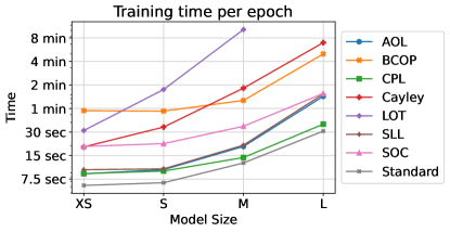
Figure 2: Training time per epoch (on CIFAR-10) for different methods and different model sizes.

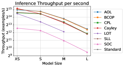
Figure 3: Inference throughput for different methods as a function of their size for CIFAR-10 sizes input images. All parameter transformations have been evaluated and cached beforehand

Figure 2 plots the training time per epoch of the different models as a function of their size, while Figure 3 plots the corresponding inference throughput for the various sizes as described in Section 4. As described in Table 5, the model base width, referred to as $w$, is doubled from one model size to the next. We expect the training and inference time to scale with $w$ similarly to how individual layers scale with their number of channels, $c$ (in Table 1). This is because the width of each of the 5 blocks of our architecture is a constant multiple of the base width, $w$.

The training time

increases (at most) about linearly with $w$ for standard convolutions, whereas the computational complexity of each single convolution scales like $c^{2}$. This suggests that parallelism on the GPU and the overhead from other operations (activations, parameter updates, etc.) are important factors determining the training time. This also explains why CPL (doing two convolutions, with identical kernel parameters) is only slightly slower than a standard convolution, and SOC (doing 5 convolutions) is only about 3 times slower than the standard convolution. The AOL and SLL methods also require times comparable to a standard convolution for small models, although eventually, the $c^{3}$ term in the computation of the rescaling makes them slower for larger models. Finally, Cayley, LOT, and BCOP methods take much longer training times per epoch. For Cayley and LOT this behavior was expected, as they have a large $\mathcal{O}(s^{2}c^{3})$ term in their computational complexity. See Table 1 for further details.

At inference time

transformations of the weights are cached, therefore some methods (AOL, BCOP) do not have any overhead compared to a standard convolution. As expected, other methods (CPL, SLL, and SOC) that apply additional convolutions to the input suffer from a corresponding overhead. Finally, Cayley and LOT have a slightly different throughput due to their FFT-based convolution. Among them, Cayley is about twice as fast because it involves a real-valued FFT rather than a complex-valued one. From Figure 3, it can be noted that cached Cayley and CPL have the same inference time, even though CPL uses twice the number of convolutions. We believe this is due to the fact that the conventional FFT-based convolution is quite efficient for large filters, but PyTorch implements a faster algorithm, i.e., Winograd, [17], that can be up to $2.5$ times faster.

5.2 Training memory requirements

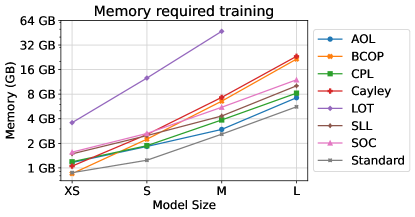
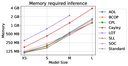
Figure 4: Memory required at training and inference time for input size $32\times 32$.

The training and inference memory requirements of the various models (measured as described in Section 4.1) are reported in Figure 4 as a function of the model size. The results of the theoretical analysis reported in Table 1 suggest that the training memory requirements always have a term linear in the number of channels, $c$ (usually the activations from the forward pass), as well as a term quadratic in $c$ (usually the weights and all transformations applied to the weights during the forward pass). This behavior can also be observed from Figure 4. For some of the models, the memory required approximately doubles from one model size to the next one, just like the width. This means that the linear term dominates (for those sizes), which makes those models relatively cheap to scale up. For the BCOP, LOT, and Cayley methods, the larger coefficients in the $c^{2}$ term (for LOT and Cayley the coefficient is even dependent on the input size, $s^{2}$) cause this term to dominate. This makes it much harder to scale those methods to more parameters. Method LOT requires huge amounts of memory, in particular LOT-L is too large to fit in 80GB GPU memory.

Note that at test time, the memory requirements are much lower, because the intermediate activation values do not need to be stored, as there is no backward pass. Therefore, at inference time, most methods require a very similar amount of memory as a standard convolution. The Cayley and LOT methods require more memory since perform the calculation in the Fourier space, as they create an intermediate representation of the weight matrices of size $\mathcal{O}(s^{2}c^{2})$.

5.3 Certified robust accuracy

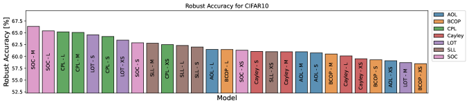
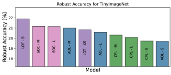
Figure 5: Certified robust accuracy by decreasing order. Note that the axes do not start at 0. For CIFAR-100 and Tiny ImageNet only the 10 best performing models are shown.

Table 2: Certified robust accuracy for radius $\epsilon=36/255$ on the evaluated datasets. Training is performed for $24$ hours.

	Accuracy [%]				Robust Accuracy [%]
Methods	XS	S	M	L	XS	S	M	L
CIFAR-10
AOL	71.7	73.6	73.4	73.7	59.1	60.8	61.0	61.5
BCOP	71.7	73.1	74.0	74.6	58.5	59.3	60.5	61.5
CPL	74.9	76.1	76.6	76.8	62.5	64.2	65.1	65.2
Cayley	73.1	74.2	74.4	73.6	59.5	61.1	61.0	60.1
LOT	75.5	76.6	72.0	-	63.4	64.6	58.7	-
SLL	73.7	74.2	75.3	74.3	61.0	62.0	62.8	62.3
SOC	74.1	75.0	76.9	76.9	61.3	62.9	66.3	65.4
CIFAR-100
AOL	40.3	43.4	44.3	41.9	27.9	31.0	31.4	29.7
BCOP	41.4	42.8	43.7	42.2	28.4	30.1	31.2	29.2
CPL	42.3	-	45.2	44.3	30.1	-	33.2	32.1
Cayley	42.3	43.9	43.5	42.9	29.2	30.5	30.5	29.5
LOT	43.5	45.2	42.8	-	30.8	32.5	29.6	-
SLL	41.4	42.8	42.4	42.1	28.9	30.5	29.9	29.6
SOC	43.1	45.2	47.3	46.2	30.6	32.6	34.9	33.5
Tiny ImageNet
AOL	26.6	29.3	30.3	30.0	18.1	19.7	21.0	20.6
BCOP	22.4	26.2	27.6	27.0	13.8	16.9	17.2	16.8
CPL	28.3	29.3	29.8	30.3	18.9	19.7	20.3	20.1
Cayley	27.8	29.6	30.1	27.2	17.9	19.5	19.3	16.7
LOT	30.7	32.5	28.8	-	20.8	21.9	18.1	-
SLL	25.1	27.0	26.5	27.9	16.6	18.4	17.7	18.8
SOC	28.9	28.8	32.1	32.1	18.9	18.8	21.2	21.1

The results related to the accuracy and the certified robust accuracy for the different methods, model sizes, and datasets measured on a $24$h training budget are summarized in Table 2. The differences among the various model sizes are also highlighted in Figure 5 by reporting the sorted values of the certified robust accuracy. Further tables and plots relative to different training budgets can be found in Appendix G. The reader can compare our results with the state-of-the-art certified robust accuracy summarized in Appendix D. However, it is worth noting that, to reach state-of-the-art performance, authors often carry out experiments using large model sizes and long training times, which makes it hard to compare the methods themselves. On the other hand, the evaluation proposed in this paper allows a fairer comparison among the different methods, since it also considers timing and memory aspects. This restriction based on time, rather than the number of epochs, ensures that merely enlarging the model size does not lead to improved performance, as bigger models typically process fewer epochs of data. Indeed, in our results in Figure 5 it is usually the M (and not the L) model that performs best. To assign a score that combines the performance of the methods over all the three datasets, we sum the number of times that each method is ranked in the first position, in the top-3, and top-10 positions. In this way, top-1 methods are counted three times, and top-3 methods are counted twice. The scores in the radar-plot shown in Figure 1 are based on those values.

Among all methods, SOC achieved a top-1 robust accuracy twice and a top-3 one 6 times, outperforming all the other methods. CPL ranks twice in the top-3 and 9 times in the top-10 positions, showing that it generally has a more stable performance compared with other methods. LOT achieved the best certified robust accuracy on Tiny ImageNet, appearing further $5$ times in the top-10. AOL did not perform very well on CIFAR-10, but reached more competitive results on Tiny ImageNet, ending up in the top-10 a total of $5$. An opposite effect can be observed for SLL, which performed reasonably well on CIFAR-10, but not so well on the two datasets with more classes, placing in the top-10 only once. This result is tied with BCOP, which also has only one model in the top-10. Finally, Cayley is consistently outperformed by the other methods. The very same analysis can be applied to the clean accuracy, whose sorted bar-plots are reported in Appendix G, where the main difference is that Cayley performs slightly better for that metric. Furthermore, it is worth highlighting that CPL is sensitive to weight initialization. We faced numerical errors during the $10$h and $24$h training of the small model on CIFAR-100.

6 Conclusions and Guidelines

This work presented a comparative study of state-of-the-art 1-Lipschitz layers under the lens of different metrics, such as time and memory requirements, accuracy, and certified robust accuracy, all evaluated at training and inference time. A theoretical comparison of the methods in terms of time and memory complexity was also presented and validated by experiments.

Taking all metrics into account (summarized in Figure 1), the results are in favor of CPL, due to its highest performance and lower consumption of computational resources. When large computational resources are available and the application does not impose stringent timing constraints during inference and training, the SOC layer could be used, due to its slightly better performance. Finally, those applications in which the inference time is crucial may take advantage of AOL or BCOP, which do not introduce additional runtime overhead (during inference) compared to a standard convolution.

Technical Appendix of “1-Lipschitz Layers Compared: Memory, Speed, and Certifiable Robustness”

Appendix A Spectral norm and orthogonalization

A lot of recently proposed methods do rely on a way of parameterizing orthogonal matrices or parameterizing matrices with bounded spectral norm. We present methods that are frequently used below:

Bjorck & Bowie [4]

introduced an iterative algorithm that finds the closest orthogonal matrix to the given input matrix. In the commonly used form, this is achieved by computing a sequence of matrices using

$$A_{k+1}=A_{k}\left(I+\frac{1}{2}Q_{k}\right),\quad\mbox{for }Q_{k}=I-A_{k}^{\top}A_{k}$$ (9)

where $A_{0}=A$, is the input matrix. The algorithm is usually truncated after a fixed number of steps, during training often $3$ iterations are enough, and for inference more (e.g. $15$) iterations are used to ensure a good approximation. Since the algorithm is differentiable, it can be applied to construct $1$-Lipschitz networks as proposed initially in [1] or also as an auxiliary method for more complex strategies [22].

Power Method

The power method was used in [26], [19] and [25] in order to bound the spectral norm of matrices.

It starts with a random initialized vector $\textbf{u}_{0}$, and iteratively applies the following:

$$\textbf{v}_{k+1}=\frac{W^{\top}\textbf{u}_{k}}{\|W^{\top}\textbf{u}_{k}\|_{2}},\quad\textbf{u}_{k+1}=\frac{W\textbf{v}_{k+1}}{\|W\textbf{v}_{k+1}\|_{2}}.$$ (10)

Then the sequence $\sigma_{k}$ converges to the spectral norm of $W$, for $\sigma_{k}$ given by

$$\sigma_{k}=\textbf{u}_{k}^{\top}W\textbf{v}_{k}.$$ (11)

This procedure allows us to obtain the spectral norm of matrices, but it can also be efficiently extended to find the spectral norm of the Jacobian of convolutional layers. This was done for example by [12, 19], using the fact that the transpose of a convolution operation (required to calculate Equation 10) is a convolution as well, with a kernel that can be constructed from the original one by transposing the channel dimensions and flipping the spatial dimensions of the kernel.

When the power method is used on a parameter matrix of a layer, we can make it even more efficient with a simple trick. We usually expect the parameter matrix to change only slightly during each training step, so we can store the result $\textbf{u}_{k}$ during each training step, and start the power method with this vector as $\textbf{u}_{0}$ during the following training step. With this trick it is enough to do a single iteration of the power method at each training step. The power method is usually not differentiated through.

Fantasic Four

proposed, in [29], allows upper bounding the Lipschitz constant of a convolution. The given bound is generally not tight, so using the method directly does not give good results. Nevertheless, since various methods require a way of bounding the spectral norm to have convergence guarantees, Fantastic Four is often used.

Appendix B Algorithms omitted in the main paper

Observe that the strategies presented in [8, 23, 26, 20, 41, 14, 36] have intentionally not been compared for different reasons. In the works presented in [8, 23], the Lipschitz constraint was solely used during training and no guarantees were provided that the resulting layers are $1$-Lipschitz. The method proposed in [26] has been extended by Fantastic 4 [29] and, indeed, can only be used as an auxiliary method to upper-bound the Lispchitz constant. The method proposed in [20] only works for linear layers and can be thought of as a special case of SOC (described in Section 2). We will give detailed reasons for the other methods below.

ONI

The method ONI [14] proposed the orthogonalization used in LOT. They parameterize orthogonal matrices as $(VV^{\top})^{-\frac{1}{2}}V$, and calculate the inverse square root using Newton’s iterations. They use this methods to define $1$-Lipschitz linear layers. However, the extension to convolutions only uses a simple unrolling, and does not provide a tight bound in general. Therefore, we did not include the method in the paper.

ECO

Explicitly constructed orthogonal (ECO) convolutions [41] also do use properties of the Fourier domain in order to parameterize a convolution. However, they do not actually calculate the convolution in the Fourier domain, but instead parameterize a layer in the Fourier domain, and then use an inverse Fourier transformation to obtain a kernel from this parameterization. We noticed, however, that the implementation provided by the authors does not produce $1$-Lipschitz layers (at least with our architecture), as can be seen in Figure 6. There, we report the batch activation variance (defined in Appendix F) as well as the spectral norm of each layer. The batch activation variance should be non-increasing for $1$-Lipschitz layers (also see Appendix F), however, for ECO this is not the case. Also, power iteration shows that the Lipschitz constant of individual layers is not $1$. Therefore we do not report this method in the main paper.

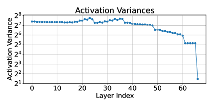
Figure 6: Left: Variance of a validation batch over the batch dimension. For $1$-Lipschitz layers, this property should be non-increasing, as proven in Appendix F. Right: Upper bound on the Lipschitz Constant applying the power method to every linear layer, and multiplying the results. Plot for ECO on CIFAR-10, with model S.

Sandwich

The authors of [36] introduced the Sandwich layer. It considers a layer of the form

$$l(x)=\sqrt{2}A^{T}\Psi\mathrm{ReLU}\left(\sqrt{2}\Psi^{-1}Bx+b\right),$$ (12)

for $\sigma$ typically the ReLU activation. The authors propose a (simultaneous) parameterization of $A$ and $B$, based on the Cayley Transform, that guarantees the whole layer to be $1$-Lipschitz. They also extend the idea to convolutions. However, for this they require to apply two Fourier transformations as well as two inverse ones. During the training of the models within the Sandwich layers, a severe vanishing gradient phenomena happens. We summarize the Frobenious norm of the gradient, obtained by inspecting the inner blocks during the training, in Table 3. For this reason we did not report the results in the main paper.

Table 3: Vanishing Gradient Phenomena of Sandwhich Layer. ConvNetXS model has been tested with a small batch size (32). Training of deeper layers (i.e., layers that are close to the input of the network) is tough due to the almost zero gradients.

Layer name	Output Shape	Gradient Norm
First Conv ($1\times 1$ kernel size)	$(32,16,32,32)$	3,36${}\cdot{}$10-7
Activation	$(32,16,32,32)$	3,36${}\cdot{}$10-7
Downsize Block($3$)	$(32,32,16,16)$	3,79${}\cdot{}$10-6
Downsize Block($3$)	$(32,64,8,8)$	5,56${}\cdot{}$10-5
Downsize Block($3$)	$(32,128,4,4)$	7,83${}\cdot{}$10-4
Downsize Block($3$)	$(32,256,2,2)$	8,15${}\cdot{}$10-3
Downsize Block($1$)	$(32,512,1,1)$	1,04${}\cdot{}$10-1
Flatten	$(32,512)$	1,04${}\cdot{}$10-1
Linear	$(32,512)$	1,82${}\cdot{}$10-1
First Channels	$(32,10)$	1,82${}\cdot{}$10-1

Appendix C Computation Complexity and Memory Requirement

In this section we give some intuition of the values in Table 1.

Recall that we consider a layer with input size $s\times s\times c$, and kernel size $k\times k$, batch size $b$, and (for some layers) we will denote the number of inner iterations by $t$.

We also use $C=bs^{2}c^{2}k^{2}$ and $M=bs^{2}c$ and $P=c^{2}k^{2}$.

AOL:

In order to compute the rescaling matrix for AOL, we need to convolve the kernel with itself. This operation has complexity $\mathcal{O}(c^{3}k^{4})$. It outputs a tensor of size $c\times c\times(2k-1)\times(2k-1)$, so in total we require memory of about $5P$ for the parameter as well as the transformation.

BCOP:

For BCOP we only require a single convolution as long as we know the kernel. However, we do require a lot of computation to create the kernel for this convolution. In particular, we require $2k-1$ matrix orthogonalizations (usually done with Bjorck & Bowie), as well as $\mathcal{O}(k^{3})$ matrix multiplications for building up the kernel. These require about $c^{3}kt+c^{3}k^{3}$ MACS as well as $c^{2}kt+c^{2}k^{3}$ memory.

Cayley:

Cayley Convolutions make use of the fact that circular padded convolutions are vector-matrix products in the Fourier domain. Applying the fast Fourier transform to inputs and weights has complexity of $\mathcal{O}(bcs^{2}\log(s^{2}))$ and $\mathcal{O}(c^{2}s^{2}\log(s^{2}))$. Then, we need to orthogonalize $\frac{1}{2}s^{2}$ matrices. Note that the factor of $\frac{1}{2}$ appears due to the fact that the Fourier transform of a real matrix has certain symmetry properties, and we can use that fact to skip half the computations. Doing the matrix orthogonalization with the Cayley Transform requires taking the inverse of a matrix, as well as matrix multiplication, the whole process has a complexity of about $s^{2}c^{3}$. The final steps consists of doing $\frac{1}{2}bs^{2}$ matrix-vector products, requiring $\frac{1}{2}bs^{2}c^{2}$ MACS, as well as another fast Fourier transform . Note that under our assumption that $c>\log(s^{2})$, the fast Fourier transform operation is dominated by other operations. Cayley Convolutions require padding the kernel from a size of $c\times c\times k\times k$ to a (usually much larger) size of $c\times c\times s\times s$ requiring a lot of extra memory. In particular we need to keep the output of the (real) fast Fourier transform, the matrix inversion as well as the matrix multiplication in memory, requiring about $\frac{1}{2}s^{2}c^{2}$ memory each.

CPL:

CPL applies two convolutions as well as an activation for each layer. They also use the Power Method (on the full convolution), however, its computational cost is dominated by the application of the convolutions.

LOT:

Similar to Cayley, LOT performs the convolution in Fourier space. However, instead of using the Cayley transform, they parameterize orthogonal matrices as $V(V^{T}V)^{-\frac{1}{2}}$. To find the inverse square root, authors relay on an iterative Newton Method. In details, let $Y_{0}=V^{T}V$ and $Z_{0}=I$, then $Y_{i}$ defined as

$$Y_{i+1}=\frac{1}{2}Y_{i}\left(3I-Z_{i}Y_{i}\right),\quad Z_{i+1}=\frac{1}{2}\left(3I-Z_{i}Y_{i}\right)Z_{i},$$ (13)

converges to $(V^{T}V)^{-\frac{1}{2}}$. Executing this procedure, includes computing $4s^{2}t$ matrix multiplications, requiring about $4s^{2}c^{3}t$ MACS as well as $4s^{2}c^{2}t$ memory.

SLL:

Similar to CPL, each SLL layer also requires evaluating two convolutions as well as one activation. However, SLL also needs to compute the AOL rescaling, resulting in total computational cost of $2C+\mathcal{O}(c^{3}k^{4})$.

SOC:

For each SOC layer we require applying $t$ convolutions. Other required operations (application of Fantastic 4 for an initial bound, as well as parameterizing the kernel such that the Jacobian is skew-symmetric) are cheap in comparison.

Appendix D Comparison with SOTA

In this section, we report state-of-the-art results from the literature. In contrast to our comparison, the runs reported often use larger architectures and longer training times. Find results in Table Tab. 4.

Table 4: SOTA from the literature on CIFAR-10 sorted by publication date (from older to newer). Readers can note that there is a clear trend of increasing the model dimension to achieve higher robust accuracy.

		Certifiable Accuracy [%]				Number of
Method	Std.Acc [%]	$\varepsilon=\frac{36}{255}$	$\varepsilon=\frac{72}{255}$	$\varepsilon=\frac{108}{255}$	$\varepsilon=1$	Parameters
BCOP Large [22]	72.1	58.2	-	-	-	2M
Cayley KW-Large [34]	75.3	59.1	-	-	-	2M
SOC LipNet-25 [30]	76.4	61.9	-	-	-	24M
AOL Large [28]	71.6	64.0	56.4	49.0	23.7	136M
LOT LipNet-25 [40]	76.8	64.4	49.8	37.3	-	27M
SOC LipNet-15 + CRC [31]	79.4	67.0	52.6	38.3	-	21M
CPL XL [25, Table1]	78.5	64.4	48.0	33.0	-	236M
SLL X-Large [2]	73.3	65.8	58.4	51.3	27.3	236M

Appendix E Experimental Setup

In addition to theoretically analyzing different proposed layers, we also do an empirical comparison of those layers. In order to allow for a fair and meaningful comparison, we try to fix the architecture, loss function and optimizer, and evaluate all proposed layers with the same setting.

From the data in Table 1 we know that different layers will have very different throughputs. In order to have a fair comparison despite of that, we limit the total training time instead of fixing a certain amount of training epochs. We report results of training for 2h, 10h as well as 24h.

We describe the chosen setting below.

E.1 Architecture

Table 5: Architecture. It depends on width parameter $w$, kernel size $k$ ($k\in\{1,3\}$) and the number of classes $c$. For details of the Downsize Block see Tab. 6.

Layer name	Output size
Input	$32\times 32\times 3$
Zero Channel Padding	$32\times 32\times w$
Conv ($1\times 1$ kernel size)	$32\times 32\times w$
Activation	$32\times 32\times w$
Downsize Block($k$)	$16\times 16\times 2w$
Downsize Block($k$)	$8\times 8\times 4w$
Downsize Block($k$)	$4\times 4\times 8w$
Downsize Block($k$)	$2\times 2\times 16w$
Downsize Block($1$)	$1\times 1\times 32w$
Flatten	$32w$
Linear	$32w$
First Channels($c$)	$c$

Table 6: Downsize Block($k$) with input size $s\times s\times t$:

	Layer name	Kernel size	Output size
$5\times\Big{\{}$	Conv	$k\times k$	$s\times s\times t$
	Activation	-	$s\times s\times t$
	First Channels	-	$s\times s\times t/2$
	Pixel Unshuffle	-	$s/2\times s/2\times 2t$

We show the architecture used for our experiments in Tables 5 and 6. It is a standard convolutional architecture, that doubles the number of channels whenever the resolution is reduced. Note that we exclusively use convolutions with the same input and output size as an attempt to make the model less dependent on the initialization used by the convolutional layers. We use kernel size $3$ in all our main experiments. The layer Zero Channel Padding in Table 5 just appends channels with value $0$ to the input, and the layer First Channels($c$) outputs only the first $c$ channels, and ignores the rest. Finally, the layer Pixel Unshuffle (implemented in PyTorch) takes each $2\times 2\times c$ patches of an image and reshapes them into size $1\times 1\times 4c$.

For each $1$-Lipschitz layer, we also test architectures of different sizes. In particular, we define 4 categories of models based on the number of parameters. We call those categories XS, S, M and L. See Table 7 for the exact numbers. In this table we also report the width parameter $w$ that ensures our architecture has the correct number of parameters.

Table 7: Number of parameters for different model sizes, as well as the width parameter $w$ such that the architecture in Tab. 5 has the correct size.

Size	Parameters (millions)	$w$
XS	$1<p<2$	$16$
S	$4<p<8$	$32$
M	$16<p<32$	$64$
L	$\ \ 64<p<128$	$128$

Remark 2.

For most methods, the number of parameters per layer are about the same. There are two exceptions, BCOP and Sandwich. BCOP parameterizes the convolution kernel with $c$ input channels and $c$ output channels using a matrix of size $c\times c$ and $2(k-1)$ matrices of size $c\times c/2$. Therefore, the number of parameters of a convolution using BCOP is $kc^{2}$, less than the $k^{2}c^{2}$ parameters of a plain convolution. The Sandwich layer has about twice as many parameters as the other layers for the same width, as it parameterizes two weight matrices, $A$ and $B$ in Equation 12, per layer.

E.2 Loss function

We use the loss function proposed by [28], with the temperature parameter set to the value used there ($t=1/4$). Our goal metric is certified robust accuracy for perturbation of maximal size $\epsilon=36/255$. We aim at robustness of maximal size $2\epsilon$ during training. In order to achieve that we set the margin parameter to $2\sqrt{2}\epsilon$.

E.3 Optimizer

We use SGD with a momentum of 0.9 for all experiments. We also used a learning rate schedule. We choose to use OneCycleLR, as described by [32], with default values as in PyTorch. We set the batch size to 256 for all experiments.

E.4 Training Time

On of our main goals is to evaluate what is the best model to use given a certain time budget. In order to do this, we measure the time per epoch as described in Section 4.1 on an A100 GPU with 80GB memory for different methods and different model sizes. Then we estimate the number of epochs we can do in our chosen time budget of either $2$h, $10$h or $24$h, and use that many epochs to train our models. The amount of epochs corresponding to the given time budget is summarized in Table 8.

Table 8: Budget of training epochs for different model sizes, layer types and datasets. Batch size and training time are set to be $256$ and $2$h respectively for all the architectures.

	CIFAR				TinyImageNet
	XS	S	M	L	XS	S	M	L
AOL	837	763	367	83	223	213	123	34
BCOP	127	125	94	24	50	50	39	11
CPL	836	797	522	194	240	194	148	63
Cayley	356	214	70	17	138	86	30	8
ECO	399	387	290	162	142	131	95	54
LOT	222	68	11	-	83	29	5	-
SLL	735	703	353	79	242	194	118	32
SOC	371	336	201	77	122	87	63	27
Param.s (M)	1.57	6.28	25.12	100.46	1.58	6.29	25.16	100.63

BCOP has less parameters overall, see Remark 2.

E.5 Hyperparameter Random Search

The learning rate and weight decay for each setting (model size, method and dataset) was tuned on the validation set. For each method we did hyperparameter search by training for $2h$ (corresponding number of epochs in Table 8). We did 16 runs with learning-rate of the form $10^{x}$, where $x$ is sampled uniformly in the interval $[-4,-1]$, and with weight-decay of the form $10^{x}$, where $x$ is sampled uniformly in the interval $[-5.5,-3.5]$. Finally, we selected the learning rate and weight decay corresponding to the run with the highest validation certified robust accuracy for radius $36/255$. We use these hyperparameters found also for the experiments with longer training time.

E.6 Datasets

We evaluate on three different datasets, CIFAR-10, CIFAR-100 [16] and Tiny ImageNet [18].

For CIFAR-10 and CIFAR-100 we use the architecture described in Table 5. Since the architectures are identical, so are time- and memory requirements, and therefore also the epoch budget. As preprocessing we subtract the dataset channel means from each image. As data augmentation at training time we apply random crops (4 pixels) and random flipping.

In order to assess the behavior on larger images, we replicate the evaluation on the Tiny ImageNet dataset [18]: a subset of $200$ classes of the ImageNet [11] dataset, with images scaled to have size $64\times 64$.

In order to allow for the larger input size of this dataset, we add one additional Downsize Block to our model. We also divide the width parameter (given in Table 7) by 2 to keep the amount of parameters similar. We again subtract the channel mean for each image. As data augmentation we we us RandAugment [10] with $2$ transformations of magnitude $9$ (out of $31$).

E.7 Metrics

As described in Section 4.1 we evaluate the methods in terms of three main metrics. The throughput, the memory requirements as well and the certified robust accuracy a model can achieve in a fixed amount of time.

The evaluation of the throughput is performed on an NVIDIA A100 80GB PCIe GPU . We measure it by averaging the time it takes to process $100$ batches (including forward pass, backward pass and parameter update), and use this value to calculate the average number of examples a model can process per second. In order to estimate the inference throughput, we first evaluate and cache all calculations that do not depend on the input (such as power iterations on the weights). With this we measure the average time of the forward pass of $100$ batches, and calculate the throughput from that value.

Appendix F Batch Activation Variance

As one (simple to compute) sanity check that the models we train are actually $1$-Lipschitz, we consider the batch activation variance. For layers that are $1$-Lipschitz, we show below that the batch activation variance cannot increase from one layer to the next. This gives us a mechanism to detect (some) issues with trained models, including numerical ones, conceptual ones as well as problems in the implementation.

To compute the batch activation variance we consider a mini-batch of inputs, and for this mini-batch we consider the outputs of each layer. Denote the outputs of layer $l$ as $a_{1}^{(l)},\dots,a_{b}^{(l)}$, where $b$ is the batch size. Then we set

$$\mu^{(l)}=\frac{1}{b}\sum_{i=1}^{b}a_{i}^{(l)}$$ (14)

$$\operatorname{BatchVar}_{l}=\frac{1}{b}\sum_{i=1}^{b}\|a_{i}^{(l)}-\mu^{(l)}\|_{2}^{2},$$ (15)

where the $l_{2}$ norm is calculated based on the flattened tensor. Denote layer $l$ as $f_{l}$. Then we have that

$$\operatorname{BatchVar}_{l+1} =\frac{1}{b}\sum_{i=1}^{b}\|a_{i}^{(l+1)}-\mu^{(l+1)}\|_{2}^{2}$$ (16)

$$\leq\frac{1}{b}\sum_{i=1}^{b}\|f_{l}(a_{i}^{(l)})-f_{l}(\mu^{(l)})\|_{2}^{2}$$ (17)

$$\leq\frac{1}{b}\sum_{i=1}^{b}\|a_{i}^{(l)}-\mu^{(l)}\|_{2}^{2}$$ (18)

$$=\operatorname{BatchVar}_{l}.$$ (19)

Here, for the first inequality we use that (by definition) $a_{i}^{(l+1)}=f_{l}(a_{i}^{(l)})$ and that the term $\sum_{i=1}^{n}\|a_{i}^{(l+1)}-x\|_{2}^{2}$ is minimal for $x=\mu^{(l+1)}$. The second inequality follows from the $1$-Lipschitz property. The equation above shows that the batch activation variance can not increase from one layer to the next for $1$-Lipschitz layers. Therefore, if we see an increase in experiments that shows that the layer is not actually $1$-Lipschitz.

As a further check that the layers are $1$-Lipschitz we also apply (convolutional) power iteration to each linear layer after training.

Appendix G Further Experimental Results

In this section, further experiments –not presented in the main paper— can be found.

G.1 Different training time budgets

In this section we report the experimental results for three different training budgets: $2h$, $10h$ and $24h$. See the results in Table 9 (CIFAR-10), Table 10 (CIFAR-100), and Table 11 (Tiny ImageNet). Each of those tables also reports the best learning rate and weight decay found by the random search for each setting.

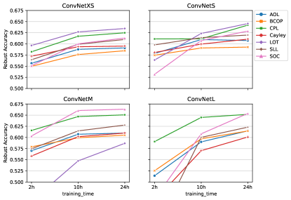
Figure 7: Line plots of the robust accuracy for various methods where models are training with different time budgets

Furthermore, a different representation of the impact of the training time on the robust accuracy can be found in Figure 7.

G.2 Time and Memory Requirements on Tiny ImageNet

See plot Fig. 8 for an evaluation of time and memory usage for Tiny ImageNet dataset. The models used on CIFAR-10 and the ones on Tiny ImageNet are identical up to one convolutional block, therefore also the results in Figure 8 are similar to the results on CIFAR-10 reported in the main paper.

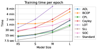
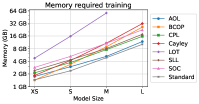
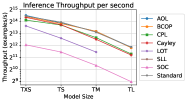
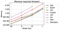
Figure 8: Measured time and memory requirements on Tiny ImageNet.

G.3 Kernel size $1\times 1$

For CIFAR-10 dataset, we tested models where convolutional layers have a kernel size of $1\times 1$, to evaluate if the quicker epoch time can compensate for the lower number of parameters. In almost all cases the answer was negative, the version with $3\times 3$ kernel outperformed the one with the $1\times 1$ kernel.We therefore do not recommend reducing the kernel size. See Table 12 for a detailed view of the accuracy and robust accuracy.

G.4 Clean Accuracy

As a reference, we plotted the accuracy of different models in Figure 9. The rankings by accuracy are similar to the rankings by certified robust accuracy. One difference is that the Cayley method performs better relative to other methods when measured in terms of accuracy.

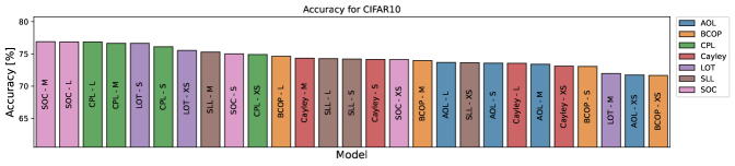
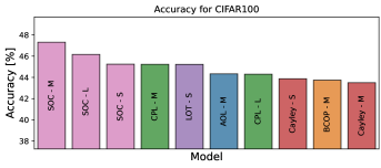
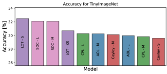
Figure 9: Barplots of models sorted by decreasing clean accuracy. For CIFAR-100 and Tiny ImageNet only the 10 best performing models are shown.

Appendix H Issues and observations

As already thoroughly analyzed in the dedicated section, some of the known methods in the literature have been omitted in the main paper since we faced serious concerns. Nevertheless, we also encountered some difficulties during the implementation of the methods that we did report in the main paper. The aim of this section is to highlight these difficulties, we hope this can open a constructive debate.

1. In the SLL [2] code, taken from the authors’ repository, there is no attention to numerical errors that can easily happen from close-to-zero divisions during the parameter transformation. We solve the issue, by adopting the commonly used strategy, i.e. we included a factor of 1${}\cdot{}$10^-6 while dividing for the AOL-rescaling of the weight matrix. Furthermore, the code provided in the SLL repository only works for a kernel size of $3$, we fixed the issue in our implementation.

2. The CPL method [25] features a high sensitivity to the initialization of the weights. Long training, e.g. 24-hour training, can sometimes result in NaN during the update of the weights. In that case we re-ran the models with different seeds.

3. Furthermore, there was no initialization method stated in the CPL paper, and also no code was provided. Therefore, we used the initialization from the similar SLL method.

4. During the training of Sandwich we faced some numerical errors. To investigate such errors, we tested a lighter version of the method — without the learnable rescaling $\Psi$ — for the reason described in Remark 3, which shows that the rescaling $\Psi$ inside the layer can be embedded into the bias term and hence the product $\Psi\Psi^{-1}$ can be omitted.

5. Similarly, for SLL, the matrix $Q$ in Equation 8 does not add additional degrees of freedom to the model. Instead of having parameters $W$, $Q$ and $b$ we could define and optimize over $P=WQ^{-1}$ and $\tilde{b}=Q^{-1}b$. However, for our experiments we used the original parameterization.

6. The method Cayley [34], in the form proposed in the original paper, does not cache the — costly — transformation of the weight matrix whenever the layer is in inference mode. We fix this issue in our implementation.

7. The LOT method, [40], leverages $10$ inner iterations for both training and inference in order to estimate the inverse of the square root with their proposed Newton-like method. Since the gradient is tracked for the whole procedure, the amount of memory required during the training is prohibitive for large models. Furthermore, since the memory is required for the parameter transformation, reducing the batch size does not solve this problem. In order to make the Large model (L) fit in the memory, we tested the LOT method with only $2$ inner iterations. However, the performance in terms of accuracy and robust accuracy is not comparable to other strategies, hence we omitted it from our tables.

Remark 3.

The learnable parameter $\Psi$ of the sandwich layer corresponds to a scaling of the bias. In details, for each parameters $A,B,b$ and $\Psi=\mathrm{diag}\left(e^{d_{i}}\right)$ there exists a rescaling of the bias $\tilde{b}$ such that

$$l(x)=\sqrt{2}A^{T}\Psi\mathrm{ReLU}\left(\sqrt{2}\Psi^{-1}Bx+b\right)=\sqrt{2}A^{T}\mathrm{ReLU}\left(\sqrt{2}Bx+\tilde{b}\right)$$ (20)

Proof.

Observing that for each $\alpha>0$ and $x\in\mathbb{R}$, $\mathrm{ReLU}\left(\alpha x\right)=\alpha\mathrm{ReLU}\left(x\right)$, and that

$$\forall\mathbf{x}\in\mathbb{R}^{n},\quad\Psi^{-1}\mathbf{x}=\begin{bmatrix}e^{-d_{1}}x_{1}\\ \vdots\\ e^{-d_{n}}x_{n}\end{bmatrix},$$

the following identity holds

$$l(x) =\sqrt{2}A^{T}\Psi\mathrm{ReLU}\left(\sqrt{2}\Psi^{-1}Bx+b\right)$$ (21)

$$=\sqrt{2}A^{T}\Psi\mathrm{ReLU}\left(\sqrt{2}\Psi^{-1}\left(\sqrt{2}Bx+\Psi b\right)\right)$$

$$=\sqrt{2}A^{T}\Psi\Psi^{-1}\mathrm{ReLU}\left(\sqrt{2}Bx+\Psi b\right)$$

$$=\sqrt{2}A^{T}\mathrm{ReLU}\left(\sqrt{2}Bx+\Psi b\right).$$

Considering $\tilde{b}=\Psi b$ concludes the proof. ∎

Appendix I Code

We often build on code provided with the original papers. This includes

• https://github.com/berndprach/AOL (AOL)

• https://github.com/ColinQiyangLi/LConvNet (BCOP)

• https://github.com/locuslab/orthogonal-convolutions (Cayley)

• https://github.com/AI-secure/Layerwise-Orthogonal-Training (LOT)

• https://github.com/acfr/LBDN (Sandwich)

• https://github.com/araujoalexandre/Lipschitz-SLL-Networks (SLL)

• https://github.com/singlasahil14/SOC (SOC)

We are grateful for authors providing code to the research community.

Table 9: Standard and Robust Accuracy on CIFAR-10. We also report the best learning rate and weight decay found by a random search.

				Accuracy [%]			Robust Accuracy [%]
			Training Time	2h	10h	24h	2h	10h	24h
Layer	Model	LR	WD
AOL	XS	6${}\cdot{}$10-2	4${}\cdot{}$10-5	68.5	71.7	71.7	55.6	58.8	59.1
	S	1${}\cdot{}$10-2	5${}\cdot{}$10-5	70.9	73.0	73.6	57.9	61.0	60.8
	M	2${}\cdot{}$10-2	1${}\cdot{}$10-4	70.3	73.4	73.4	57.0	60.7	61.0
	L	2${}\cdot{}$10-2	7${}\cdot{}$10-5	64.7	71.8	73.7	51.4	59.0	61.5
BCOP	XS	7${}\cdot{}$10-3	3${}\cdot{}$10-4	69.0	70.8	71.7	55.0	57.6	58.5
	S	4${}\cdot{}$10-3	8${}\cdot{}$10-5	70.6	72.5	73.1	57.5	59.1	59.3
	M	6${}\cdot{}$10-3	7${}\cdot{}$10-6	71.8	73.6	74.0	57.9	59.9	60.5
	L	1${}\cdot{}$10-3	9${}\cdot{}$10-6	67.6	73.2	74.6	52.5	59.7	61.5
CPL	XS	3${}\cdot{}$10-2	1${}\cdot{}$10-4	71.7	74.3	74.9	58.2	61.7	62.5
	S	7${}\cdot{}$10-2	1${}\cdot{}$10-4	73.9	74.1	76.1	61.1	61.1	64.2
	M	8${}\cdot{}$10-2	1${}\cdot{}$10-4	74.3	76.4	76.6	61.6	64.7	65.1
	L	5${}\cdot{}$10-2	3${}\cdot{}$10-4	72.6	76.5	76.8	59.1	64.5	65.2
Cayley	XS	2${}\cdot{}$10-2	2${}\cdot{}$10-5	71.3	73.2	73.1	57.2	59.4	59.5
	S	1${}\cdot{}$10-2	1${}\cdot{}$10-5	71.9	73.6	74.2	58.1	60.0	61.1
	M	1${}\cdot{}$10-2	6${}\cdot{}$10-6	70.2	73.5	74.4	55.8	60.2	61.0
	L	8${}\cdot{}$10-3	2${}\cdot{}$10-4	61.3	71.1	73.6	45.9	57.0	60.1
LOT	XS	8${}\cdot{}$10-2	4${}\cdot{}$10-6	73.5	75.2	75.5	59.6	62.7	63.4
	S	3${}\cdot{}$10-2	7${}\cdot{}$10-5	70.5	75.0	76.6	56.4	62.3	64.6
	M	2${}\cdot{}$10-2	9${}\cdot{}$10-6	61.4	69.3	72.0	45.7	54.7	58.7
SLL	XS	9${}\cdot{}$10-2	2${}\cdot{}$10-5	69.9	73.1	73.7	56.4	59.9	61.0
	S	4${}\cdot{}$10-2	2${}\cdot{}$10-4	72.9	74.0	74.2	59.8	61.4	62.0
	M	9${}\cdot{}$10-2	9${}\cdot{}$10-5	70.5	74.4	75.3	57.4	61.5	62.8
	L	6${}\cdot{}$10-2	2${}\cdot{}$10-4	56.7	72.7	74.3	38.9	60.0	62.3
SOC	XS	5${}\cdot{}$10-2	7${}\cdot{}$10-6	68.9	72.9	74.1	55.1	60.0	61.3
	S	2${}\cdot{}$10-2	2${}\cdot{}$10-5	67.3	73.3	75.0	53.2	60.8	62.9
	M	7${}\cdot{}$10-2	1${}\cdot{}$10-4	73.1	77.0	76.9	60.3	66.0	66.3
	L	2${}\cdot{}$10-2	2${}\cdot{}$10-4	62.3	73.8	76.9	46.2	60.8	65.4

Table 10: Standard and Robust Accuracy on CIFAR-100. We also report the best learning rate and weight decay found by a random search.

				Accuracy [%]			Robust Accuracy [%]
			Training Time	2h	10h	24h	2h	10h	24h
Layer	Model	LR	WD
AOL	XS	3${}\cdot{}$10-2	1${}\cdot{}$10-4	37.9	40.1	40.3	26.6	28.0	27.9
	S	2${}\cdot{}$10-2	2${}\cdot{}$10-5	40.5	43.4	43.4	29.0	30.8	31.0
	M	7${}\cdot{}$10-2	6${}\cdot{}$10-6	40.5	43.5	44.3	28.4	31.1	31.4
	L	6${}\cdot{}$10-2	4${}\cdot{}$10-5	34.5	41.1	41.9	23.1	29.2	29.7
BCOP	XS	8${}\cdot{}$10-3	3${}\cdot{}$10-4	35.4	40.0	41.4	22.9	27.8	28.4
	S	6${}\cdot{}$10-3	3${}\cdot{}$10-4	37.8	42.1	42.8	24.5	29.5	30.1
	M	2${}\cdot{}$10-3	2${}\cdot{}$10-4	37.6	43.8	43.7	24.6	30.4	31.2
	L	4${}\cdot{}$10-3	1${}\cdot{}$10-5	29.2	40.3	42.2	17.3	27.2	29.2
CPL	XS	9${}\cdot{}$10-2	3${}\cdot{}$10-5	39.7	42.0	42.3	27.9	29.8	30.1
	S	9${}\cdot{}$10-2	2${}\cdot{}$10-4	42.1	1.0	1.0	29.8	0.0	0.0
	M	4${}\cdot{}$10-2	4${}\cdot{}$10-5	40.5	44.5	45.2	27.4	32.4	33.2
	L	9${}\cdot{}$10-2	2${}\cdot{}$10-4	40.1	43.9	44.3	27.3	31.5	32.1
Cayley	XS	4${}\cdot{}$10-2	2${}\cdot{}$10-5	41.1	41.6	42.3	27.9	29.2	29.2
	S	2${}\cdot{}$10-2	1${}\cdot{}$10-4	42.3	43.1	43.9	28.8	30.4	30.5
	M	6${}\cdot{}$10-3	4${}\cdot{}$10-6	38.6	43.3	43.5	25.3	29.9	30.5
	L	5${}\cdot{}$10-3	2${}\cdot{}$10-5	26.3	40.3	42.9	14.3	27.0	29.5
LOT	XS	6${}\cdot{}$10-2	3${}\cdot{}$10-4	42.7	43.8	43.5	29.4	30.9	30.8
	S	5${}\cdot{}$10-2	2${}\cdot{}$10-4	40.3	45.2	45.2	27.2	31.8	32.5
	M	4${}\cdot{}$10-2	9${}\cdot{}$10-5	28.4	38.9	42.8	15.5	25.9	29.6
SLL	XS	5${}\cdot{}$10-2	6${}\cdot{}$10-5	37.9	40.9	41.4	25.9	29.0	28.9
	S	1${}\cdot{}$10-1	7${}\cdot{}$10-5	40.0	41.9	42.8	28.4	29.9	30.5
	M	7${}\cdot{}$10-2	2${}\cdot{}$10-4	39.3	41.9	42.4	27.0	30.0	29.9
	L	9${}\cdot{}$10-2	8${}\cdot{}$10-5	22.0	38.5	42.1	10.8	26.4	29.6
SOC	XS	7${}\cdot{}$10-2	2${}\cdot{}$10-4	40.7	43.1	43.1	27.7	29.7	30.6
	S	9${}\cdot{}$10-2	1${}\cdot{}$10-4	42.2	44.5	45.2	29.3	31.9	32.6
	M	4${}\cdot{}$10-2	3${}\cdot{}$10-4	41.8	46.2	47.3	28.8	33.5	34.9
	L	7${}\cdot{}$10-2	3${}\cdot{}$10-5	34.7	43.1	46.2	21.5	30.2	33.5

Table 11: Experimental results on the TinyImageNet dataset.

				Accuracy [%]			Robust Accuracy [%]
			Training Time	2h	10h	24h	2h	10h	24h
Layer	Model	LR	WD
AOL	XS	3${}\cdot{}$10-2	2${}\cdot{}$10-5	24.5	26.9	26.6	16.5	18.4	18.1
	S	7${}\cdot{}$10-2	5${}\cdot{}$10-6	24.9	27.3	29.3	16.8	18.5	19.7
	M	4${}\cdot{}$10-2	8${}\cdot{}$10-6	26.2	29.5	30.3	18.1	20.4	21.0
	L	2${}\cdot{}$10-2	8${}\cdot{}$10-6	22.1	27.7	30.0	12.8	18.8	20.6
BCOP	XS	6${}\cdot{}$10-4	5${}\cdot{}$10-5	11.7	20.4	22.4	4.7	11.6	13.8
	S	7${}\cdot{}$10-4	4${}\cdot{}$10-5	19.0	25.3	26.2	10.1	15.7	16.9
	M	3${}\cdot{}$10-4	1${}\cdot{}$10-4	20.0	25.4	27.6	10.5	15.8	17.2
	L	1${}\cdot{}$10-4	3${}\cdot{}$10-4	9.6	23.6	27.0	2.6	14.0	16.8
CPL	XS	1${}\cdot{}$10-1	9${}\cdot{}$10-6	26.5	27.5	28.3	16.3	17.5	18.9
	S	4${}\cdot{}$10-2	3${}\cdot{}$10-5	26.2	29.3	29.3	16.7	19.4	19.7
	M	4${}\cdot{}$10-2	2${}\cdot{}$10-5	26.3	29.4	29.8	16.7	19.5	20.3
	L	6${}\cdot{}$10-2	1${}\cdot{}$10-5	24.7	29.8	30.3	15.0	19.2	20.1
Cayley	XS	8${}\cdot{}$10-3	8${}\cdot{}$10-5	25.3	27.5	27.8	15.7	17.9	17.9
	S	5${}\cdot{}$10-3	7${}\cdot{}$10-5	25.6	29.3	29.6	15.8	19.1	19.5
	M	4${}\cdot{}$10-3	4${}\cdot{}$10-5	20.2	29.2	30.1	9.9	18.8	19.3
	L	1${}\cdot{}$10-3	3${}\cdot{}$10-4	5.7	22.1	27.2	0.9	11.9	16.7
LOT	XS	3${}\cdot{}$10-2	2${}\cdot{}$10-4	28.1	31.1	30.7	18.2	20.4	20.8
	S	5${}\cdot{}$10-2	1${}\cdot{}$10-4	27.1	32.0	32.5	16.3	21.6	21.9
	M	2${}\cdot{}$10-2	6${}\cdot{}$10-6	12.6	25.2	28.8	4.6	14.5	18.1
SLL	XS	7${}\cdot{}$10-2	3${}\cdot{}$10-4	24.2	25.3	25.1	14.9	16.7	16.6
	S	4${}\cdot{}$10-2	2${}\cdot{}$10-4	24.4	25.7	27.0	15.6	16.8	18.4
	M	5${}\cdot{}$10-2	5${}\cdot{}$10-5	17.0	26.2	26.5	7.8	17.0	17.7
	L	7${}\cdot{}$10-2	1${}\cdot{}$10-4	11.4	26.2	27.9	2.9	16.7	18.8
SOC	XS	9${}\cdot{}$10-2	1${}\cdot{}$10-4	25.5	28.7	28.9	15.7	18.7	18.9
	S	7${}\cdot{}$10-2	2${}\cdot{}$10-5	23.9	28.4	28.8	14.0	18.5	18.8
	M	7${}\cdot{}$10-2	1${}\cdot{}$10-4	25.7	31.1	32.1	15.5	20.4	21.2
	L	6${}\cdot{}$10-2	1${}\cdot{}$10-4	20.3	30.1	32.1	10.1	19.7	21.1

Table 12: Kernel size $1\times 1$, on CIFAR-10, for different time budgets. We report accuracy and certified robust accuracy for radius $\epsilon=36/355$, as well as the best learning rate and weight decay found by a random search.

				Accuracy [%]			Robust Accuracy [%]
			Training Time	2h	10h	24h	2h	10h	24h
Layer	Model	LR	WD
AOL	XS	8${}\cdot{}$10-2	7${}\cdot{}$10-6	66.5	67.9	68.0	52.1	53.9	54.3
	S	5${}\cdot{}$10-2	4${}\cdot{}$10-5	67.7	69.0	69.7	53.7	55.1	55.6
	M	2${}\cdot{}$10-2	1${}\cdot{}$10-4	67.5	69.4	70.0	54.1	55.7	56.7
	L	3${}\cdot{}$10-2	8${}\cdot{}$10-5	64.3	68.7	69.6	50.0	54.8	56.1
BCOP	XS	1${}\cdot{}$10-2	7${}\cdot{}$10-5	65.3	67.5	68.6	51.3	53.4	54.5
	S	4${}\cdot{}$10-3	2${}\cdot{}$10-5	66.9	69.1	69.5	52.6	54.3	55.4
	M	8${}\cdot{}$10-3	5${}\cdot{}$10-6	67.3	69.8	70.3	52.8	55.5	56.1
	L	4${}\cdot{}$10-3	2${}\cdot{}$10-4	64.0	68.6	69.6	48.9	54.3	55.8
BnB	XS	8${}\cdot{}$10-3	1${}\cdot{}$10-4	66.1	66.3	66.4	52.1	51.2	51.5
	S	2${}\cdot{}$10-2	2${}\cdot{}$10-5	67.9	69.8	69.7	53.1	55.8	55.3
	M	2${}\cdot{}$10-2	4${}\cdot{}$10-6	67.5	70.3	71.0	52.8	56.0	56.8
	L	3${}\cdot{}$10-2	2${}\cdot{}$10-4	66.0	66.2	61.0	51.5	51.7	45.5
CPL	XS	2${}\cdot{}$10-2	1${}\cdot{}$10-4	69.2	71.5	72.0	55.5	58.6	59.1
	S	9${}\cdot{}$10-2	9${}\cdot{}$10-5	70.6	71.2	10.0	57.8	58.2	0.0
	M	1${}\cdot{}$10-1	2${}\cdot{}$10-4	69.7	10.0	10.0	56.1	0.0	0.0
	L	8${}\cdot{}$10-2	9${}\cdot{}$10-6	67.8	72.3	73.8	54.0	59.4	61.1
Cayley	XS	1${}\cdot{}$10-2	2${}\cdot{}$10-5	65.3	67.4	67.9	50.7	52.9	53.8
	S	1${}\cdot{}$10-2	4${}\cdot{}$10-6	65.9	68.4	68.8	51.3	53.8	54.5
	M	2${}\cdot{}$10-2	2${}\cdot{}$10-5	63.5	67.5	69.1	48.8	53.4	55.0
	L	2${}\cdot{}$10-2	8${}\cdot{}$10-5	57.4	64.7	67.2	41.4	49.9	52.9
LOT	XS	2${}\cdot{}$10-2	2${}\cdot{}$10-4	65.8	68.0	69.3	51.1	53.9	54.9
	S	5${}\cdot{}$10-2	3${}\cdot{}$10-4	60.0	68.1	68.8	44.4	54.3	54.5
SLL	XS	4${}\cdot{}$10-2	1${}\cdot{}$10-4	67.9	70.2	10.0	54.8	57.3	0.0
	S	3${}\cdot{}$10-2	2${}\cdot{}$10-4	69.1	70.4	10.0	55.9	57.1	0.0
	M	7${}\cdot{}$10-2	2${}\cdot{}$10-4	69.0	10.0	10.0	55.5	0.0	0.0
	L	9${}\cdot{}$10-2	2${}\cdot{}$10-4	62.9	69.5	69.8	48.7	55.6	56.1
SOC	XS	7${}\cdot{}$10-2	2${}\cdot{}$10-5	65.0	67.2	67.5	49.2	52.1	52.3
	S	4${}\cdot{}$10-2	6${}\cdot{}$10-6	65.4	68.1	68.7	49.9	52.5	54.2
	M	3${}\cdot{}$10-2	7${}\cdot{}$10-5	66.0	69.2	70.5	50.5	54.3	55.6
	L	4${}\cdot{}$10-2	9${}\cdot{}$10-5	64.0	69.2	70.4	48.5	54.3	55.9

References

- [1] Cem Anil, James Lucas, and Roger Grosse. Sorting out Lipschitz function approximation. In International Conference on Machine Learing (ICML), 2019.
- [2] Alexandre Araujo, Aaron J Havens, Blaise Delattre, Alexandre Allauzen, and Bin Hu. A unified algebraic perspective on Lipschitz neural networks. In International Conference on Learning Representations (ICLR), 2023.
- [3] Battista Biggio, Igino Corona, Davide Maiorca, Blaine Nelson, Nedim Šrndić, Pavel Laskov, Giorgio Giacinto, and Fabio Roli. Evasion attacks against machine learning at test time. In Machine Learning and Knowledge Discovery in Databases, 2013.
- [4] Å. Björck and C. Bowie. An iterative algorithm for computing the best estimate of an orthogonal matrix. SIAM Journal on Numerical Analysis, 1971.
- [5] Fabio Brau, Giulio Rossolini, Alessandro Biondi, and Giorgio Buttazzo. Robust-by-design classification via unitary-gradient neural networks. Proceedings of the AAAI Conference on Artificial Intelligence, 2023.
- [6] Nicholas Carlini, Florian Tramer, Krishnamurthy Dj Dvijotham, Leslie Rice, Mingjie Sun, and J Zico Kolter. (Certified!!) adversarial robustness for free! In International Conference on Learning Representations (ICLR), 2023.
- [7] Arthur Cayley. About the algebraic structure of the orthogonal group and the other classical groups in a field of characteristic zero or a prime characteristic. Journal für die reine und angewandte Mathematik, 1846.
- [8] Moustapha Cisse, Piotr Bojanowski, Edouard Grave, Yann Dauphin, and Nicolas Usunier. Parseval networks: Improving robustness to adversarial examples. In International conference on machine learning, 2017.
- [9] Jeremy Cohen, Elan Rosenfeld, and Zico Kolter. Certified adversarial robustness via randomized smoothing. In Proceedings of the 36th International Conference on Machine Learning, 2019.
- [10] Ekin D Cubuk, Barret Zoph, Jonathon Shlens, and Quoc V Le. Randaugment: Practical automated data augmentation with a reduced search space. In Proceedings of the IEEE/CVF conference on computer vision and pattern recognition workshops, 2020.
- [11] Jia Deng, Wei Dong, Richard Socher, Li-Jia Li, Kai Li, and Li Fei-Fei. Imagenet: A large-scale hierarchical image database. In Conference on Computer Vision and Pattern Recognition (CVPR), 2009.
- [12] Farzan Farnia, Jesse Zhang, and David Tse. Generalizable adversarial training via spectral normalization. In International Conference on Learning Representations, 2018.
- [13] Emiel Hoogeboom, Victor Garcia Satorras, Jakub Tomczak, and Max Welling. The convolution exponential and generalized Sylvester flows. In Advances in Neural Information Processing Systems, 2020.
- [14] Lei Huang, Li Liu, Fan Zhu, Diwen Wan, Zehuan Yuan, Bo Li, and Ling Shao. Controllable orthogonalization in training DNNs. In Conference on Computer Vision and Pattern Recognition (CVPR), 2020.
- [15] Guy Katz, Clark Barrett, David L Dill, Kyle Julian, and Mykel J Kochenderfer. Reluplex: An efficient SMT solver for verifying deep neural networks. In International conference on computer aided verification, 2017.
- [16] Alex Krizhevsky. Learning multiple layers of features from tiny images. Technical report, 2009.
- [17] Andrew Lavin and Scott Gray. Fast algorithms for convolutional neural networks. In Proceedings of the IEEE conference on computer vision and pattern recognition, 2016.
- [18] Ya Le and Xuan Yang. Tiny imagenet visual recognition challenge. CS 231N, 2015.
- [19] Klas Leino, Zifan Wang, and Matt Fredrikson. Globally-robust neural networks. In International Conference on Machine Learning, 2021.
- [20] Mario Lezcano-Casado and David Martínez-Rubio. Cheap orthogonal constraints in neural networks: A simple parametrization of the orthogonal and unitary group. In International Conference on Machine Learing (ICML), 2019.
- [21] Linyi Li, Tao Xie, and Bo Li. Sok: Certified robustness for deep neural networks. In 2023 IEEE Symposium on Security and Privacy (SP), 2023.
- [22] Qiyang Li, Saminul Haque, Cem Anil, James Lucas, Roger B Grosse, and Joern-Henrik Jacobsen. Preventing gradient attenuation in Lipschitz constrained convolutional networks. In Conference on Neural Information Processing Systems (NeurIPS), 2019.
- [23] Shuai Li, Kui Jia, Yuxin Wen, Tongliang Liu, and Dacheng Tao. Orthogonal deep neural networks. IEEE Transactions on Pattern Analysis and Machine Intelligence, 2021.
- [24] Max Losch, David Stutz, Bernt Schiele, and Mario Fritz. Certified robust models with slack control and large Lipschitz constants. arXiv preprint arXiv:2309.06166, 2023.
- [25] Laurent Meunier, Blaise J Delattre, Alexandre Araujo, and Alexandre Allauzen. A dynamical system perspective for Lipschitz neural networks. In International Conference on Machine Learing (ICML), 2022.
- [26] Takeru Miyato, Toshiki Kataoka, Masanori Koyama, and Yuichi Yoshida. Spectral normalization for generative adversarial networks. In International Conference on Learning Representations (ICLR), 2018.
- [27] Adam Paszke, Sam Gross, Francisco Massa, Adam Lerer, James Bradbury, Gregory Chanan, Trevor Killeen, Zeming Lin, Natalia Gimelshein, Luca Antiga, Alban Desmaison, Andreas Kopf, Edward Yang, Zachary DeVito, Martin Raison, Alykhan Tejani, Sasank Chilamkurthy, Benoit Steiner, Lu Fang, Junjie Bai, and Soumith Chintala. Pytorch: An imperative style, high-performance deep learning library. In Conference on Neural Information Processing Systems (NeurIPS). 2019.
- [28] Bernd Prach and Christoph H Lampert. Almost-orthogonal layers for efficient general-purpose Lipschitz networks. In European Conference on Computer Vision (ECCV), 2022.
- [29] S Singla and S Feizi. Fantastic four: Differentiable bounds on singular values of convolution layers. In International Conference on Learning Representations (ICLR), 2021.
- [30] Sahil Singla and Soheil Feizi. Skew orthogonal convolutions. In International Conference on Machine Learing (ICML), 2021.
- [31] Sahil Singla and Soheil Feizi. Improved techniques for deterministic l2 robustness. Conference on Neural Information Processing Systems (NeurIPS), 2022.
- [32] Leslie N Smith and Nicholay Topin. Super-convergence: Very fast training of neural networks using large learning rates. In Artificial intelligence and machine learning for multi-domain operations applications, 2019.
- [33] Christian Szegedy, Wojciech Zaremba, Ilya Sutskever, Joan Bruna, Dumitru Erhan, Ian Goodfellow, and Rob Fergus. Intriguing properties of neural networks. In International Conference on Learning Representations (ICLR), 2014.
- [34] Asher Trockman and J Zico Kolter. Orthogonalizing convolutional layers with the Cayley transform. In International Conference on Learning Representations (ICLR), 2021.
- [35] Yusuke Tsuzuku, Issei Sato, and Masashi Sugiyama. Lipschitz-margin training: Scalable certification of perturbation invariance for deep neural networks. Conference on Neural Information Processing Systems (NeurIPS), 2018.
- [36] Ruigang Wang and Ian Manchester. Direct parameterization of Lipschitz-bounded deep networks. In International Conference on Machine Learing (ICML), 2023.
- [37] Lily Weng, Huan Zhang, Hongge Chen, Zhao Song, Cho-Jui Hsieh, Luca Daniel, Duane Boning, and Inderjit Dhillon. Towards fast computation of certified robustness for relu networks. In International Conference on Machine Learing (ICML), 2018.
- [38] Eric Wong and Zico Kolter. Provable defenses against adversarial examples via the convex outer adversarial polytope. In International Conference on Machine Learing (ICML), 2018.
- [39] Lechao Xiao, Yasaman Bahri, Jascha Sohl-Dickstein, Samuel Schoenholz, and Jeffrey Pennington. Dynamical isometry and a mean field theory of CNNs: How to train 10,000-layer vanilla convolutional neural networks. In International Conference on Machine Learing (ICML), 2018.
- [40] Xiaojun Xu, Linyi Li, and Bo Li. Lot: Layer-wise orthogonal training on improving l2 certified robustness. Conference on Neural Information Processing Systems (NeurIPS), 2022.
- [41] Tan Yu, Jun Li, Yunfeng Cai, and Ping Li. Constructing orthogonal convolutions in an explicit manner. In International Conference on Learning Representations (ICLR), 2021.